Multivariate state and parameter estimation with data assimilation applied to sea-ice models using a Maxwell elasto-brittle rheology

In this study, we investigate the fully multivariate state and parameter estimation through idealised simulations of a dynamics-only model that uses the novel Maxwell elasto-brittle (MEB) sea-ice rheology and in which we estimate not only the sea-ice concentration, thickness and velocity, but also its level of damage, internal stress and cohesion. Specifically, we estimate the air drag coefficient and the so-called damage parameter of the MEB model. Mimicking the realistic observation network with different combinations of observations, we demonstrate that various issues can potentially arise in a complex sea-ice model, especially in instances for which the external forcing dominates the model forecast error growth. Even though further investigation will be needed using an operational (a coupled dynamics–thermodynamics) sea-ice model, we show that, with the current observation network, it is possible to improve both the observed and the unobserved model state forecast and parameter accuracy.

1 Introduction

An accurate representation of the state of sea ice in the Arctic is important for making both short-term–seasonal and long-term climate predictions. Recent observations show that its extent is in decline and, in particular, that it is shifting from a multi-year ice type to “younger” first-year ice (Meier, 2017). This ongoing shift induces a larger year-to-year and inter-annual variability in the sea-ice extent, which makes the short-term and seasonal Arctic sea-ice forecasting even more challenging, despite its crucial relevance for shipping routes and fisheries (Mioduszewski et al., 2019). The Arctic sea ice is also a major player of the climate systems via its feedback to the Earth surface albedo, ocean and atmosphere global circulations. Accurate sea-ice simulations are therefore essential for better climate projections (Bertino and Holland, 2017).

As in other areas of environmental prediction, errors in sea-ice models can be attributed to errors either in the initial conditions or in the model representation of physical processes. Due to the low degree of internal instabilities of the sea-ice evolution on long space scales and timescales (> seasonal timescales), model error is the main source of prediction uncertainty, and it is especially detrimental to long-term forecasts needed for climate simulations. Numerical models incorporate parametrisations to represent physical processes that are not explicitly described or resolved in the model. The parameters involved can be estimated in different ways. One way is to base the parameter on values obtained from laboratory experiments in idealised environments, but this has the limitation that the selected values may not scale up for complex realistic simulations. Alternatively, one can select a value from a range of possible candidates based on which candidate produces the best fit between the model and observations (Dansereau, 2011; Miller et al., 2006; Heorton et al., 2019). Nevertheless, as the number of parameters to be tuned increases, the latter approach becomes computationally infeasible. In that case, an optimised version of the aforementioned process called “data assimilation” must be pursued.

Data assimilation (DA) combines observations with the model forecast to provide the most likely estimate for the true state and/or parameter of the system (see e.g. Carrassi et al., 2018; Evensen et al., 2022; Park and Zupanski, 2022). It has been proved to be essential for sea-ice forecasting (Sakov et al., 2012a; Lea et al., 2015; Zuo et al., 2019). Data assimilation can account for both the forecast and the observation errors in the state and/or parameter estimation. To this extent, error statistics need to be specified. In ensemble DA, the forecast error statistics are obtained from an ensemble of model runs (Evensen, 2003).

Previous studies have shown that assimilating sea-ice concentration (SIC) can reduce errors in sea-ice thickness (SIT) (Massonnet et al., 2015) and that, in coupled sea-ice and ocean models, sea-ice observations help in initialising ocean fields such as the ocean and wind forcing (Toyoda et al., 2016). Model parameters can be made part of the state, and when it is assumed that they are affected by errors, DA can be used to estimate them. An example of such an approach in sea-ice models can be found in Massonnet et al. (2014), who used the ensemble Kalman filter (EnKF; Evensen, 2003) to estimate the air drag coefficients, ocean drag coefficients and sea-ice strength parameter by assimilating sea-ice drift data.

Sea-ice models include multiple variables. However, only three of these are usually observed and assimilated: SIC, SIT and sea-ice drift. These observations are mostly obtained from satellites. In situ observations are usually only used for evaluation purposes (Jakobson et al., 2012). The satellite observations of SIC show good spatial and temporal coverage with relatively low uncertainty. Assimilation of SIC shows tremendous benefits for sea-ice forecasting (Lisæter et al., 2003; Stark et al., 2007). In the past decades, though less accurate than SIC, SIT has started to be assimilated, with further improvements to forecasts (Xie et al., 2018; Blockley and Peterson, 2018; Fiedler et al., 2022b). The assimilation of sea-ice drift has been less successful and has motivated further developments of sea-ice rheological models (Sakov et al., 2012a). These studies together show the important role of DA in sea-ice prediction.

In this study, we explore the capability of ensemble DA to estimate both the state and the key sea-ice parameters in a model endowed with a Maxwell elasto-brittle (MEB) rheology. This rheology is adopted by the neXt-generation Sea Ice Model (neXtSIM), which runs operationally on a Lagrangian grid that uses dynamical remeshing (Rampal et al., 2016). Due to the Lagrangian framework, the advection process does not require explicit calculations, and the highly multi-scale sea-ice features, especially localised features such as the so-called linear kinematic features (LKFs), which concentrate sea-ice fracturing and high deformations rates, can be easily preserved (Bouillon and Rampal, 2015). One downside of this framework, however, is that, with the changing number of model grid points in time, it poses challenges for ensemble DA. Consequently, DA approaches have been specifically designed (e.g. Aydoğdu et al., 2019; Sampson et al., 2021) and implemented in the context of neXtSIM by Cheng et al. (2023). Another drawback of using a Lagrangian framework in a sea-ice model is that coupling to existing ocean and atmospheric model components, which are virtually all Eulerian, requires the use of a coupler on a fixed exchange grid (Boutin et al., 2023).

Because such a coupling is essential for climate simulations, a new version of neXtSIM based on an Eulerian framework is being developed under the Scale-Aware Sea Ice Project (SASIP; https://sasip-climate.github.io/, last access: 7 May 2024). It is in the light of these developments that this study is inscribed. In particular, the dynamics-only sea-ice MEB model of Dansereau et al. (2016, 2017) has been designed following an Eulerian approach and a discontinuous Galerkin treatment of advection. With the aid of this dynamics-only sea-ice MEB model, we study in detail the capabilities, limitations and adaptations of ensemble DA to infer state and model parameters based on synthetic observations of the Arctic sea ice.

We intentionally use a dynamics-only model whereby thermodynamics processes are missing. Indeed, such a model is already complex enough and, on short (daily and weekly) timescales, sufficient to focus on how the mechanical/dynamical processes lead to the emergence of complex, potentially nonlinear, relations between model states, model parameters and the observable quantities. Those are the relations the DA has to rely on. Thus, although the model does not capture all of the processes at play in sea ice, we shall see how our experiments reveal a number of complex interactions. On the other hand, the use of a simpler idealised model allows us to conduct a fully multivariate estimate where we infer all model fields with only a handful of available observations, a realistic situation that has not yet been studied extensively in sea-ice DA.

The paper is organised as follows. In Sect. 2 we introduce the iterative ensemble Kalman filter (IEnKF), state-of-the-art DA approach used in this study. Then we describe the model and its configurations in Sect. 3. The ensemble DA setup and twin experiments are given in Sect. 4. Results for both multivariate state estimation in a “perfect-model” setup and parameter estimation in a biased model are reported in Sect. 5. In Sect. 6 we discuss some of the critical aspects of ensemble DA in this context together with how to address them in future works. We finally summarise our findings in Sect. 7.

2 Data assimilation: the iterative ensemble Kalman filter

The iterative ensemble Kalman filter (IEnKF; Sakov et al., 2012b; Bocquet and Sakov, 2012, 2014) is a variant of the Kalman filter (KF). Like the KF, it is constructed based on the Bayes theorem under the assumption that the prior (forecast), evidence (observation) and posterior (analysis) follow a Gaussian distribution. It has successfully been applied to joint state and model parameter estimation problems (Bocquet and Sakov, 2013; Haussaire and Bocquet, 2016; Bocquet et al., 2021). In ensemble DA methods, the linear model assumption of the KF is relaxed and the prior distribution is estimated from a finite ensemble of model forecasts. A relevant feature of the IEnKF is that it solves for the analysis via a nonlinear optimisation aimed at maximising the a posteriori probability distribution. This key aspect makes it worth investigating its performance in the context of predicting Arctic sea ice, which is characterised by strong and complex nonlinear relations as well as weak nonlinearity in the observations. The IEnKF is the filter version of the more general iterative ensemble Kalman smoother (Bocquet and Sakov, 2014), and it is conceptually a generalisation of the maximum likelihood ensemble filter by Zupanski (2005).

In an ensemble DA system consisting of N_e ensemble members with an N-dimensional state vector, the ensemble mean of the posterior analysis ${\stackrel{\mathrm{‾}}{\mathbf{x}}}^a\in {\mathbb{R}}^N$ is given by ${\stackrel{\mathrm{‾}}{\mathbf{x}}}^a={\stackrel{\mathrm{‾}}{\mathbf{x}}}^f+{\mathbf{Aw}}_{\min }$, with ${\stackrel{\mathrm{‾}}{\mathbf{x}}}^f\in {\mathbb{R}}^N$ being the a priori ensemble mean, $\mathbf{A}\in {\mathbb{R}}^{N\times N_{\mathrm{e}}}$ the matrix of ensemble anomalies with N rows and N_e columns obtained by removing the ensemble mean from the full ensemble matrix, and ${\mathbf{w}}_{\min }\in {\mathbb{R}}^{N_{\mathrm{e}}}$ the minimum of w obtained from the cost function as

$$\begin{array}{}\text{(1a)}& {\mathbf{w}}_{\min }:={\mathrm{argmin}}_{\mathbf{w}}\mathcal{J}\left(\mathbf{w}\right),\end{array}$$

with

$$\begin{array}{}\text{(1b)}& \begin{array}{rl}\mathcal{J}\left(\mathbf{w}\right)& ={\displaystyle \frac{\mathrm{1}}{\mathrm{2}}}{\left(\mathbf{y}-\mathcal{H}({\stackrel{\mathrm{‾}}{\mathbf{x}}}^f+\mathbf{Aw})\right)}^{\mathrm{T}}{\mathbf{R}}^{-\mathrm{1}}\left(\mathbf{y}-\mathcal{H}({\stackrel{\mathrm{‾}}{\mathbf{x}}}^f+\mathbf{Aw})\right)\\ & +{\displaystyle \frac{\mathrm{1}}{\mathrm{2}}}(N-\mathrm{1}){\mathbf{w}}^{\mathrm{T}}\mathbf{w},\end{array}\end{array}$$

where $\mathbf{y}\in {\mathbb{R}}^{N_{\mathrm{o}}}$ contains N_o observations whose error covariance is specified by $\mathbf{R}\in {\mathbb{R}}^{N_{\mathrm{o}}\times N_{\mathrm{o}}}$ and ℋ is the observation operator. Formulating the problem as in Eq. (1) is equivalent to an ensemble-variational method. Note that extensive reviews of these methods can be found in Chap. 7 of Asch et al. (2016), Bannister (2017) or Sect. 4 in Carrassi et al. (2018). In our implementation, the cost function in Eq. (1) is minimised using a Gauss–Newton method. The stopping criterion in this study comprises a maximum of 40 iterations for the experiments of state estimation only (Sects. 4.3.2 and 5.1) plus the constraint of $\left|\right|{\mathbf{w}}^k-{\mathbf{w}}^{k-\mathrm{1}}\left|\right|<{\mathrm{10}}^{-\mathrm{3}}$ when parameters are also estimated (Sect. 5.2–5.4). The latter additional constraint has been included on the basis of theoretical arguments and numerical experiments. It avoids overfitting at a single analysis step for parameters without time dependency. Without the additional stopping criterion, the parameter estimation leads to excessive corrections that do not appear in the case of state estimation only. The use of early stopping criteria in the context of ensemble-variational methods with domain localisation was also originally suggested by Bocquet (2016) to deal with potential convergence problems. After minimisation, the posterior analysis error covariance is approximated, via the ensemble, by the inverse of the Hessian matrix of 𝒥.

The forecast error covariance is approximated with the ensemble anomaly matrix, A, by $\frac{\mathrm{1}}{N-\mathrm{1}}{\mathbf{AA}}^{\mathrm{T}}$. Given that the state vector contains both observed and unobserved model fields, the forecast error covariance matrix contains the (ensemble-based) cross-covariance between these fields that allows for propagating the data content to all model fields, including those that are not directly observed. As we shall clarify later, we use a fully multivariate augmented DA where the state vector contains all model fields and model parameters that will be estimated (see for instance Ruiz et al., 2013). The analysis of the unobserved fields and parameters depends directly on the cross-correlations between these fields and the observations.

3 Model setup

In this study, we use a dynamics-only sea-ice model in an idealised setup. In this section, we provide details about the model setup used in our numerical experiments. This includes the model equations, its parameters and the choice of external forcing fields. The setup described in this section is used as modelled “truth” in the following DA experiments.

3.1 The dynamics-only sea-ice model

The dynamics-only sea-ice model uses the MEB rheology proposed by Dansereau et al. (2016). The model itself and its numerical implementation, based on an Eulerian, discontinuous Galerkin approach, are presented in Dansereau et al. (2017). In the MEB model, sea ice is treated as a viscous–elasto-brittle material. This rheology allows for representing the ice cover as a brittle solid where it is relatively undamaged (i.e. unfractured) and highly concentrated relative to ice-free waters and as an elastic–viscous fluid where it is intensively fractured and low in concentration. By associating sea-ice with an elastic solid rather than a highly viscous fluid and by incorporating a variable (the level of damage, d) to represent its degree of fracturing at the sub-grid scale, this model differs significantly from the widely employed (elastic–)viscous–plastic rheologies (Hunke et al., 2010).

The dynamics-only MEB sea-ice model describes the evolution of nine model fields: sea-ice concentration (SIC) A; sea-ice thickness (SIT) h; sea-ice velocity (SIV) $\mathbf{u}=(u_x,u_y)=(u,v)$; level of damage d; cohesion C; and internal stress $\mathit{\sigma }=\left(\begin{array}{ll}{\mathit{\sigma }}_{xx}& {\mathit{\sigma }}_{xy}\\ {\mathit{\sigma }}_{yx}& {\mathit{\sigma }}_{yy}\end{array}\right)$, where σ_yx=σ_xy (see Dansereau et al., 2017).

In the MEB rheology, the evolution of SIV, the level of damage and stress describes the kinematics of the sea ice. To obtain a physically plausible solution, a stress–velocity–damage constraint that respects the MEB constitutive equation (which relates SIV to σ) must be satisfied. Other model fields also enter the momentum, constitutive and damage evolution and mass conservation equations, but these are just advected by SIV. Here, we highlight the momentum and stress equations of the sea-ice model. These equations will be relevant in parameter estimation experiments. The momentum equation is given as

$$\begin{array}{}\text{(2)}& \mathit{\rho }h{\displaystyle \frac{\mathrm{D}\mathbf{u}}{\mathrm{D}t}}=\mathrm{\nabla }\cdot \left(h\mathit{\sigma }\right)+{\mathit{\rho }}_{\mathrm{a}}{C}_{\mathrm{a}}A\left|{\mathbf{u}}_{\mathrm{a}}\right|{\mathbf{u}}_{\mathrm{a}},\end{array}$$

where ρ and ρ_a are the sea ice and air density respectively, u_a is the wind field, $\frac{\mathrm{D}}{\mathrm{D}t}$ is the material derivative, and C_a is the air drag coefficient. The stress equation is

$$\begin{array}{}\text{(3)}& \begin{array}{rl}{\mathit{\lambda }}^{\mathrm{0}}{d}^{\mathit{\alpha }-\mathrm{1}}& \left[{\displaystyle \frac{\partial \mathit{\sigma }}{\partial t}}+(\mathbf{u}\cdot \mathrm{\nabla })\mathit{\sigma }+{\mathit{\beta }}_{\mathrm{a}}(\mathrm{\nabla }\mathbf{u},\mathit{\sigma })\right]\\ & +\lceil \mathrm{1}-d\rceil \mathit{\sigma }={\mathit{\eta }}^{\mathrm{0}}{d}^{\prime \mathit{\alpha }}\exp \left[-c^{*}(\mathrm{1}-A)\right]\mathbf{K}:\mathcal{D}\left(\mathbf{u}\right),\end{array}\end{array}$$

where λ⁰ is the undamaged relaxation time; β_a is a function that accounts for the effects of rotation and deformation; η⁰ is the undamaged apparent viscosity; $d^{\prime \mathit{\alpha }}=(\mathrm{1}-\frac{{\mathit{\eta }}_{\min }}{{\mathit{\eta }}_{\mathrm{0}}})d^{\mathit{\alpha }}+\frac{{\mathit{\eta }}_{\min }}{{\mathit{\eta }}_{\mathrm{0}}}$, with η_min being the minimum apparent viscosity and α being a damage-related parameter; K is a stiffness tensor; and 𝒟() is the symmetric part of the velocity gradient.

The model equations are discretised on an unstructured triangular grid using a finite-element, discontinuous Galerkin method where the sea-ice velocities are defined on triangular vertices (degree of polynomial approximations of 1) and all other model fields are defined on the face of the triangular element (degree of polynomial approximations of 0 or constant by element; see Dansereau et al., 2017). In particular, because the constitutive, momentum and level-of-damage evolution is coupled, SIV, the level of damage and sea-ice stress are solved using a semi-implicit, iterative method. Besides these dynamical properties, the sea-ice model used in this study does not include thermodynamics processes. As such, it is a short-timescale proxy for the dynamic–thermodynamic sea-ice model currently under construction in the SASIP project, neXtSIM_DG. However, this future model builds on the MEB rheology and discontinuous Galerkin-based numerical scheme. Therefore, the present model is a reliable surrogate of the dynamical components and of the numerical core of neXtSIM_DG.

The evolution of the sea-ice model is controlled by multiple model parameters which define the physical properties of the sea ice and thereby intrinsically affect the representation of sea ice in the model. These parameters (see Table A1) follow the choice in Dansereau et al. (2017) with exceptions for the spatial and temporal resolutions and minimum cohesion. In our experiments, the model runs at the spatial resolution of around 15 km and a time step of 30 s. This ensures numerical stability while sufficiently resolving the propagation of damage, the fastest process represented in the model. The model is solved on a squared model domain of $[-L,L]\times [-L,L]$ with the x and y axes aligned along the perpendicular sides of the square with L=100 km. This gives us 512 elements and 285 nodes. To enhance internal variability (and thus maintain ensemble spread in the IEnKF), the minimum sea-ice cohesion, which sets the resistance of the sea-ice cover to fracturing, is lowered to 5000 from 8000 Pa, which has been used so far in neXtSIM (Rampal et al., 2016).

In this study, the DA's ability to estimate two model parameters will be investigated: the air drag coefficient, C_a, in Eq. (2) and damage parameter, α, in Eq. (3). C_a enters the model in the momentum equation (see Eq. 2), modulating the influence of the wind fields on SIV. This parameter corresponds to the effect of external forcing on the sea-ice model. α controls the swiftness of the transition between the elasto-brittle regime at a low level of damage and the viscous regime at a high level of damage. The mechanical behaviour of an elasto-brittle solid is less predictable in nature than that of a viscous fluid (Weiss and Dansereau, 2017). This means that erroneous α changes the internal property of sea ice and influences the sea-ice predictability. The choice of the parameters to be estimated is largely based on previous studies. Massonnet et al. (2014) showed that a coupled ocean–sea-ice model is sensitive to the drag coefficient, which is estimated with the ensemble Kalman filter. Using neXtSIM, a rheology-based model similar to the MEB model used here, Rabatel et al. (2018) showed the importance of the wind stress, and thus the air drag coefficient, in determining the spread of the sea-ice trajectories. Furthermore, Cheng et al. (2020) demonstrated that the shape and orientation of the area covered by the sea-ice trajectories depend on the sea-ice air drag coefficient. Besides the drag coefficient, the damage parameter is the only other minimal parameter in a solid-like MEB rheology-based model. Drag coefficient and damage parameters are the two sole tunable parameters present in the MEB model used in this study. This is because, in a dynamics-only MEB model, the air drag coefficient and the damage parameter are the only two parameters that do not affect the maximum speed of the fastest-propagating elastic waves which influence the model stability with given time steps.

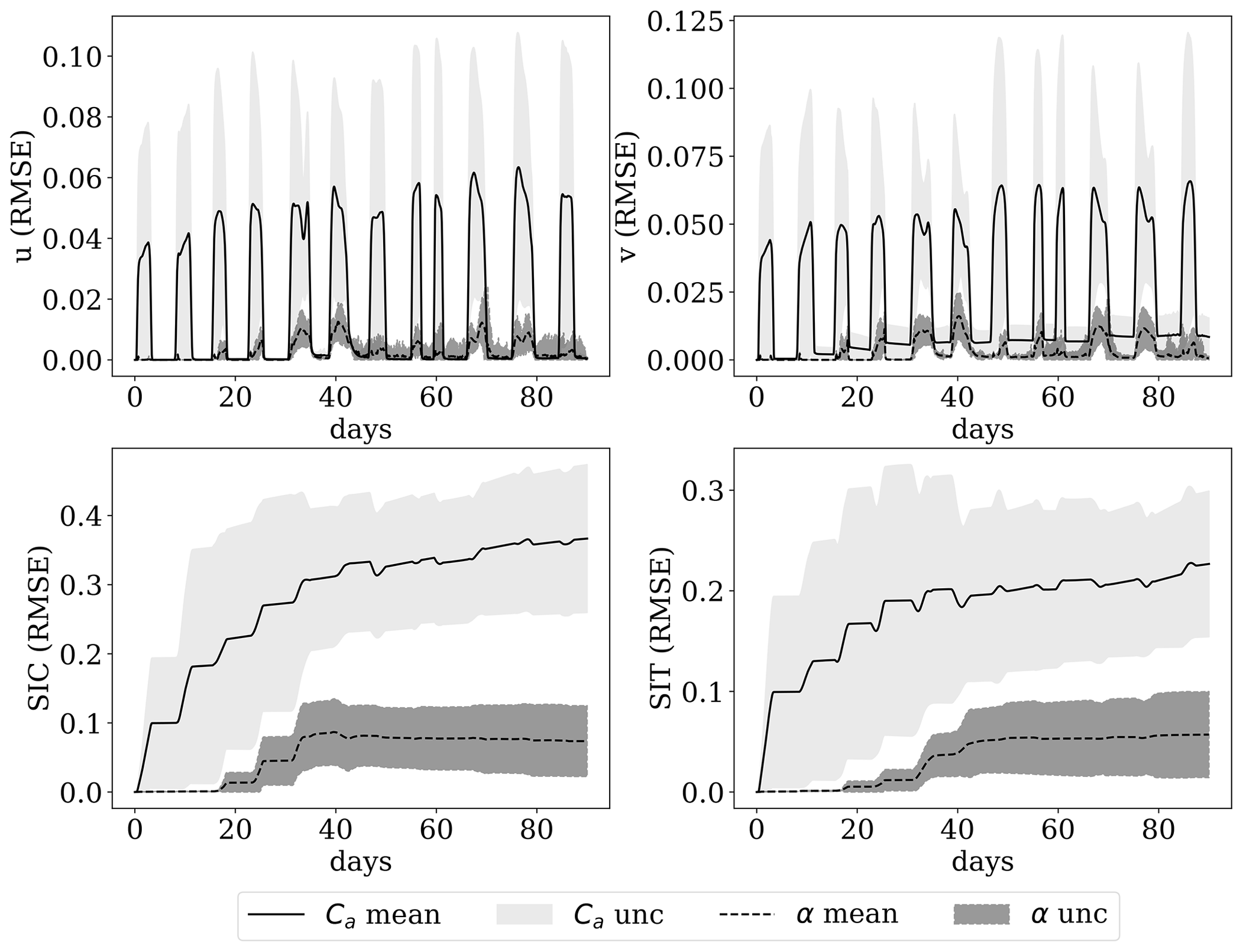
Figure 1 Sensitivity of SIV, SIC and SIT to perturbed C_a or α parameter. The shaded area is the standard deviation, a representation of uncertainty in the ensemble an indication of the strength of the sensitivity.

We have performed a numerical sensitivity analysis which shows that the observations are sensitive to both parameters. Results are shown in Fig. 1, where the same initial and boundary conditions are used while each ensemble member has different C_a or α values. The parameter values are sampled from $\mathcal{N}(\mathrm{2.5}\times {\mathrm{10}}^{-\mathrm{3}},\mathrm{5}\times {\mathrm{10}}^{-\mathrm{4}})$, and 𝒩(6,1.5) for C_a and α respectively. The model parameters are time-independent, and the ensemble means are $\mathrm{2.5}\times {\mathrm{10}}^{-\mathrm{3}}$ and 6.5 respectively. Figure 1 shows that both C_a and α have a strong impact on SIC and SIT, while a smaller effect is observed on SIV.

Table 1 The initial and boundary condition of the experimental setup in the dynamics-only sea-ice model. Here $r=\sqrt{x^{\mathrm{2}}+y^{\mathrm{2}}}$, with (x,y) being the coordinate of the grid points and r₀=50 km. The boundary condition at $y=-L=L$ is that of the fields transported into the model domain.

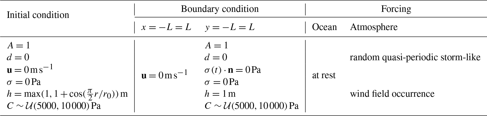
The initial and boundary conditions of the model are shown in Table 1. The simulations start with a domain covered by undamaged sea ice at rest with a random cohesion field. The value of the cohesion field for each element is sampled from a uniform distribution between 5000 and 10 000 Pa. As shown in Fig. 2e, the initial SIT (h) is a “blob” defined by a cosine function given in Table 1, which represents the naturally inhomogeneous distribution of the SIT in space. We use no-slip boundary conditions at $x=-L=L$ and Neumann boundary conditions at $y=-L=L$, where 1 m thick undamaged sea ice is transported into the domain based on SIV. To avoid an influx of sea ice with a uniform cohesion field from the domain boundaries, the cohesion field of the inflowing ice is randomly sampled from a uniform distribution between 5000 and 10 000 Pa.

3.2 The external wind field

In the model setup, following Dansereau et al. (2017), the ocean is assumed to be at rest and the sea-ice variability relies on the wind forcing. We design an external forcing in the form of a prescribed storm-like wind drag that mimics the wind field encountered in operational sea-ice DA. Consistent with reality, the wind is therefore a major source of variability in the present simulations (Guemas et al., 2016; Rabatel et al., 2018).

The storm-like wind field is inspired by the test cases for linear advection schemes in Lauritzen et al. (2012) generated by analytical formulae as outlined in Appendix B. We deem this forcing an adequate representation of the complex horizontal atmospheric flow. The wind field is updated at each model computational time step such that the sea ice is always driven by the up-to-date wind field similarly to the case where the sea-ice model is coupled to an atmospheric model.

Table 2 The parameters of the storm that served as the truth of the wind field.

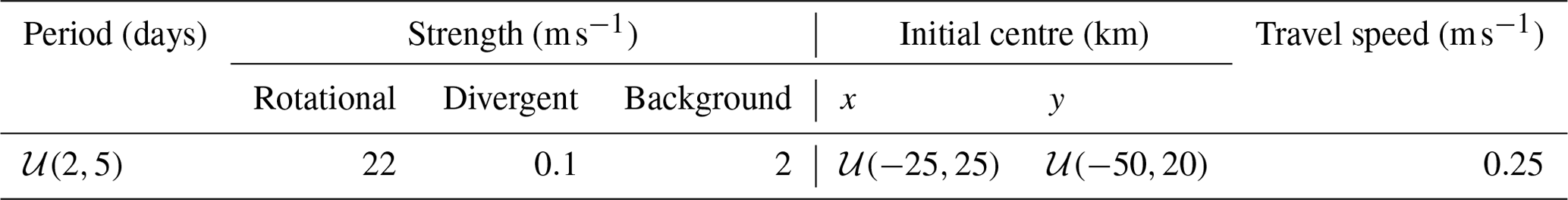
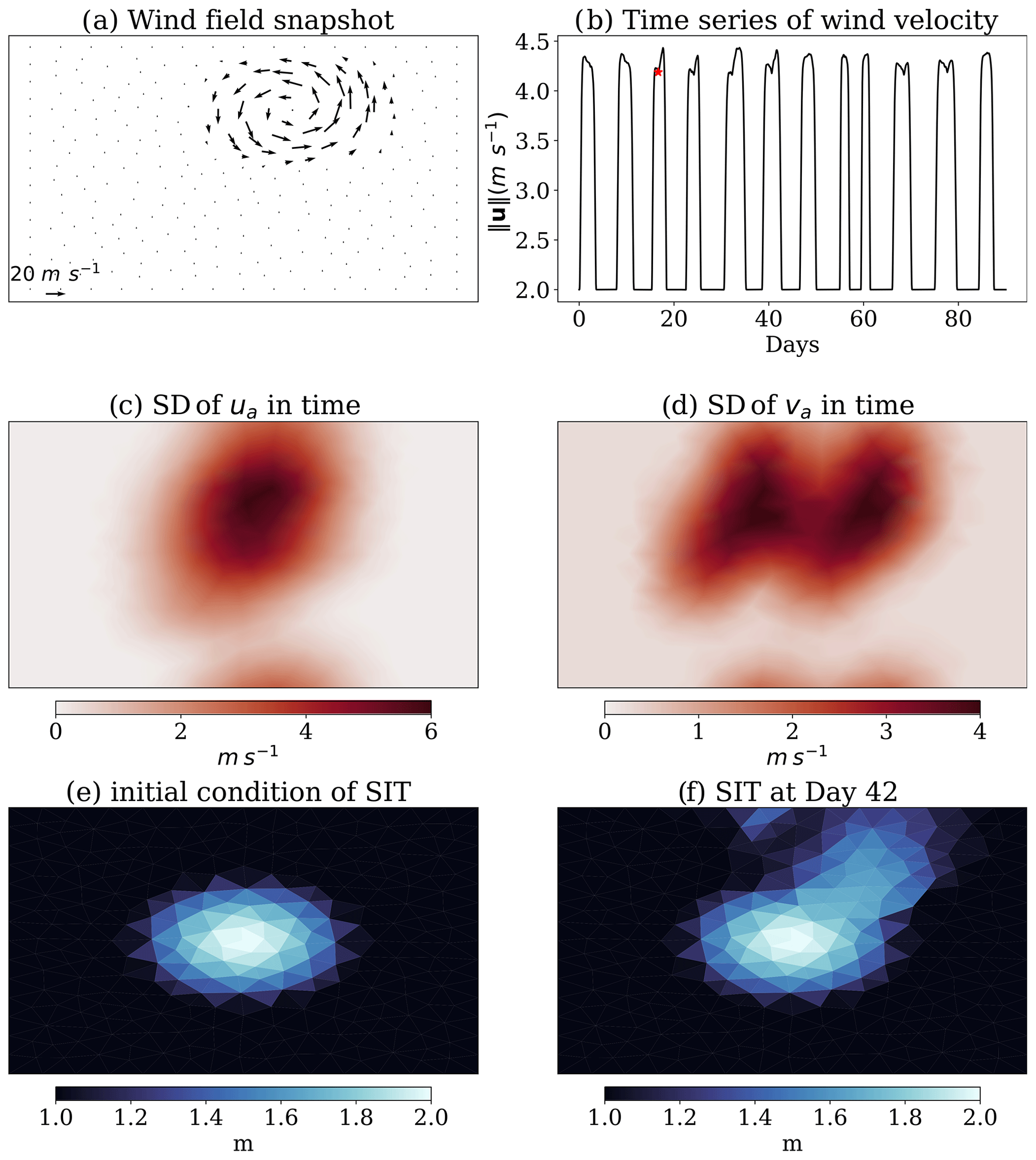
Figure 2 An illustration of the wind field and the model response in SIT. (a) A snapshot of the wind field at an arbitrary time; (b) time series of the spatially averaged wind velocity; (c) standard deviation of the u component and (d) the v component of the wind in time over 90 d; (e) the initial condition of the SIT; (f) SIT after 42 d of simulation.

The cyclone, shown in Fig. 2a, covers around a quarter of the domain in space. The wind field is superposed on a background flow (2 m s⁻¹) from the bottom to the top of the domain. The centre of the storm moves from y=0 to y=L with a speed of 0.25 m s⁻¹, which is slower than the background flow. The parameters of the storm can be found in Table 2. The formulae for the wind field also allow for a fine control of the generation and dissipation of the cyclone. Therefore, as shown in Fig. 2b, the storms (appearing as peaks in the time series) are not persistent but have time-evolving features. Following the dissipation of a cyclone, a “peaceful” period with only the background wind is used. Hence, during our 90 d experiment period, there are 12 storm occurrences. Moreover, like the duration, strength, initial centre position and travel speed of the storm are specified by the analytical formula with storm duration and initial position sampled from a uniform distribution as shown in Table 2. With the given random initial position of the storm, the variability in the wind field is confined in a limited region of the domain as shown in Fig. 2c and d. Figure 2e–f show that the variability in the wind field leads to variability in the modelled sea ice, mainly in the upper-right region of the domain as the sea ice is mostly damaged in these regions.

4 Data assimilation setup

The operational sea-ice DA corrects only the model state without dealing with model errors explicitly. It is, however, impossible to obtain a perfect model. Model errors originate from diverse sources, such as numerical discretisation, the lack of sufficient resolution as well as errors in the model parameters. We focus here on the parametric errors, as these are particularly problematic and dominate the initial conditions' errors in long-term forecasts.

As introduced in Sect. 2, the IEnKF can infer unobserved model fields thanks to its ensemble-based cross-correlations with the observed fields. This feature can also be exploited for parameter estimations. In the parameter estimation, we use the augmented approach in which the model parameters are included as part of the state vector. For example, in the case of estimating the air drag coefficient C_a, the state vector is $\mathbf{x}=(h,u,v,\mathrm{\dots },C_{\mathrm{a}}{)}^{\mathrm{T}}$. Thus their inference is ultimately related to the capability of the IEnKF to properly describe the correlation within this new, augmented virtual state composed by the physical variables and the parameters.

The simultaneous state and parameter estimation is more challenging than state estimation alone, since changes in the parameters have a direct impact and can substantially modify the model's dynamical properties. In the worst-case scenario, inappropriate parameter values can push the model through a bifurcation (a tipping point in the case of non-autonomous systems), leading to qualitatively different model behaviour than that of the data. Moreover, different parameters can have aliased uncertainties in the observed model fields, implying that not all of the parameters can be uniquely identified.

These challenges motivate the investigation of state and parameter estimation in the idealised dynamics-only sea-ice model. In this study, a series of twin experiments are conducted whereby a model run is taken to represent the truth. Synthetic observations are generated from the truth following a specified observation error distribution.

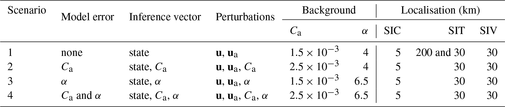
To assess DA's ability, four different scenarios are explored: (1) a perfect model where the parameters are equal to their “true” values; (2) a model with a biased air drag coefficient, C_a; (3) a model with a biased damage parameter, α; and (4) a model with biased C_a and α. A summary of the setup of each experiment is given in Table 3.

Table 3 The experiment setup used in four different scenarios. These experiments use the same truth, where u_a is the wind forcing and u(t=0) is the initial condition of SIV.

4.1 Ensemble generation

The IEnKF belongs to the category of the ensemble-based DA methods. As such it relies on an ensemble of model trajectories to approximate the forecast uncertainty. The ensemble spread represents the error in the estimate of the model state and parameters. We will explore four different scenarios, whereby, as we shall clarify later, we will employ a different strategy each time to generate the ensemble. In particular, in the cases with parametric error, each member of the ensemble will be given a different set of model parameters.

Nevertheless, in all of the four scenarios, we will perturb the wind field (i.e. an external forcing), the initial condition of the sea-ice velocity and the cohesion flux at model boundaries. The external atmospheric wind forcing is a major source of forecast uncertainty in sea-ice models. For example, Rabatel et al. (2018) and Cheng et al. (2020) studied the sensitivity of neXtSIM to the wind forcing and sea-ice cohesion. In this study, we generate synthetic perturbed wind fields around the “true wind” defined in Sect. 3.2 and use them to form an ensemble. The duration, strength, initial position and travel speed of each cyclone are perturbed with noise sampled from Gaussian distributions (see Table 4 for details). In addition to these perturbations, we also introduce a random walk for the centre of the cyclone in the zonal direction as part of the ensemble perturbation. This is generated as red noise at each time step according to

$$\begin{array}{}\text{(4)}& \mathrm{\Delta }{x}_{i+\mathrm{1}}=e^{-\mathrm{\Delta }t/\mathit{\tau }}\mathrm{\Delta }{x}_i+\mathit{ϵ},\end{array}$$

where Δx_i is the distance travelled zonally at the ith time step, τ=60 is a time decorrelation factor and ϵ is noise sampled from $\mathcal{N}(\mathrm{0},\mathrm{4.44}\times {\mathrm{10}}^{-\mathrm{5}})$ m. This red noise is not applied to the true wind. To avoid the cyclone travelling outside of our model domain, we resample the noise if the centre of the cyclone goes outside of the region between −40 and 50 km for the x coordinate. The same check and resampling are applied to the perturbations for the initial centre of the cyclone.

Table 4 Gaussian distributions of wind fields, SIV and parameter perturbations. The mean of the wind fields is given in Table 2.

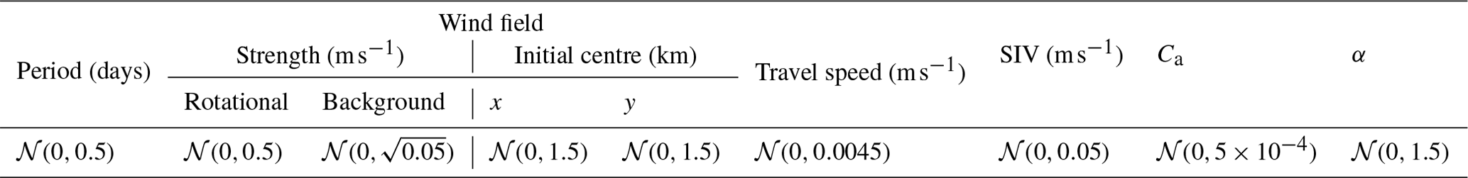
Albeit marginally with respect to variability due to the external forcing, the internal model variability caused by nonlinearities is another source of forecast error. This is accounted for in our ensemble by perturbing the SIV initial condition, in addition to perturbing the external atmospheric wind field. SIV perturbations are sampled from the Gaussian distribution, 𝒩(0,0.05). Furthermore, as discussed in Sect. 3.1, the boundary condition of the random cohesion influx, which differs for each ensemble member, adds another source of uncertainty in our experiments, but as the sea ice drifts slowly and does not travel long distances across the domain, the impact of the cohesion perturbation is limited.

In the experiments with parametric error in either C_a or α or both (experiments 2–4 in Table 3), the prior covariances of the model parameters need to be specified. As shown in Table 4, the parameter values used by the ensemble members are sampled from zero-mean Gaussian distributions with standard deviations set to be around 33 % of the true parameter value. Given that both C_a and α are bounded from below due to physical constraints, the sampled values of C_a and α are ensured to be greater than 10⁻⁵ and 2 by rejecting outliers.

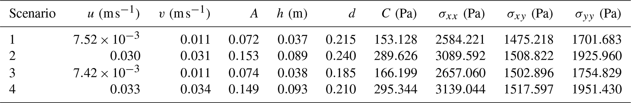
Table 5 The time- and space-averaged ensemble standard deviation of each free-run ensemble over 90 d.

4.2 Synthetic observations

Synthetic observations in our twin experiments are generated by sampling from the truth with the aim of mimicking how observations of the Arctic sea-ice are collected operationally, i.e. their spatio-temporal density.

Satellite observations of SIC, SIT and sea-ice drift are used in sea-ice forecasting and reanalysis systems (Sakov et al., 2012a). Most operational systems assimilate gridded products. However, some recent studies show the possibility of directly assimilating along-track instead of gridded data for SIT (Fiedler et al., 2022a), which could allow for a more frequent SIT assimilation than the 7 d averaged gridded products (Ricker et al., 2017) because gridded data require time for collection and processing. Hence, a star-shaped spatial distribution mimicking the along-track SIT observations is used here. For simplicity, we assume that the same star-shaped spatial distribution is available daily due to the time required for data collection from the polar satellite. Note that this treatment neglects the temporal variability in the satellite tracks. Following the protocol of gridded data, we generate synthetic observations of SIC and SIV quasi-uniformly across the model domain.

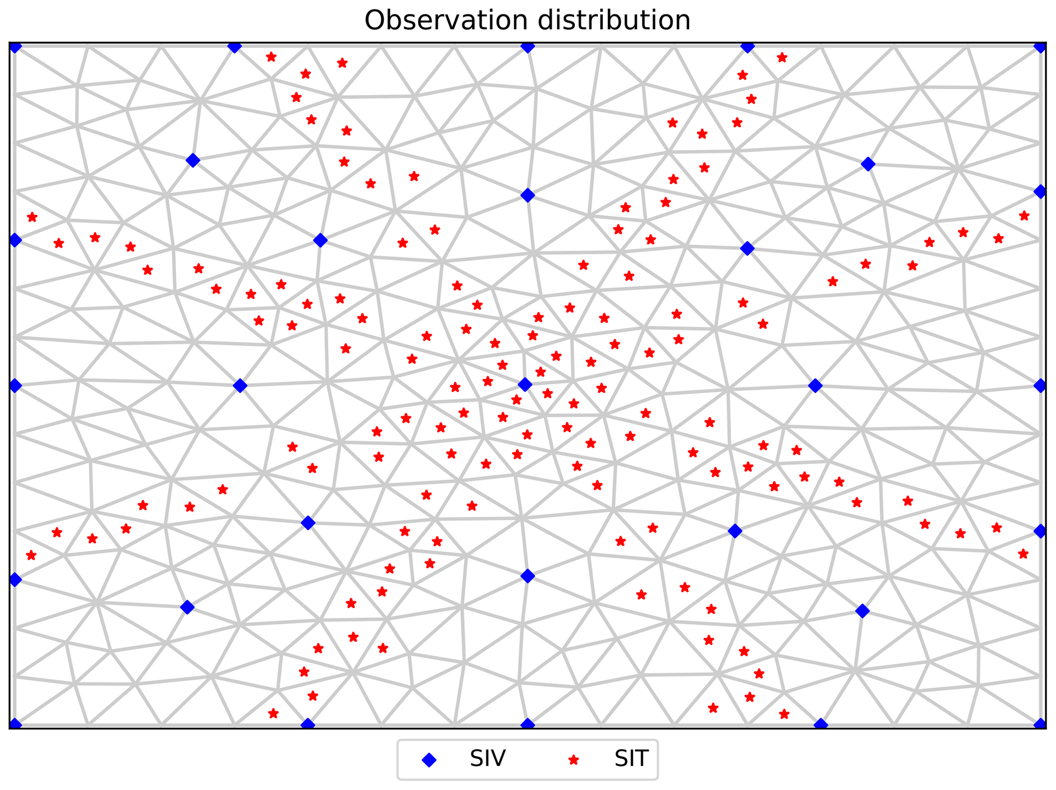
Figure 3 Observation distribution of SIT and SIV with the background triangles being the model grid. The observation distribution of SIC is not shown because it covers the entire domain.

Nowadays SIC satellite observations reach a resolution as high as 10 km. Considering that our model has a spatial resolution of around 15 km, we synthetically observe every grid point for SIC in our experiments. SIV data are sparser, with a spatial resolution of around 50 km. The position of the along-track SIT data is parametrised by four lines on the domain satisfying the condition $|y_i+c{x}_i|\le r$, where (x_i,y_i) is the spatial coordinate of the grid points, and the pair $(c,r)\in \mathit{\left\{}\right(\mathrm{2.2},\mathrm{16}\mathrm{km}),(-\mathrm{2.2},\mathrm{16}\mathrm{km}),(\mathrm{0.5},\mathrm{8}\mathrm{km}),(-\mathrm{0.5},\mathrm{8}\mathrm{km}\left)\mathit{\right\}}$. A graphic distribution of SIC and SIV can be found in Fig. 3.

The synthetic observations are generated by sampling from the truth and adding an observational error drawn from Gaussian distributions. The observation error variances of these Gaussians follow those of realistic DA systems. For SIC, we adopt the observation error standard deviation from Sakov et al. (2012a) and Cheng et al. (2023):

$$\begin{array}{}\text{(5)}& {\mathit{\sigma }}_A\left[m\right]=\sqrt{\mathrm{0.01}+(\mathrm{0.5}-|\mathrm{0.5}-A|{)}^{\mathrm{2}}}.\end{array}$$

The observation error in the along-track SIT follows the formula for the measurement uncertainty for CryoSat-2 used by Fiedler et al. (2022a):

$$\begin{array}{}\text{(6)}& {\mathit{\sigma }}_h=\left\{\begin{array}{ll}\mathrm{8}& h<\mathrm{0.7}\mathrm{m}\\ \mathrm{2}\left(\mathrm{1}-\frac{\mathrm{7}e}{\mathrm{0.3}-h^e}\right)\frac{h}{\mathrm{100}}& \mathrm{0.7}\le h<\mathrm{3}\mathrm{m}\\ \left(\mathrm{5}\left(h-\mathrm{3}\right)+\left(\mathrm{1}-\frac{\mathrm{7}e}{\mathrm{0.3}-{\mathrm{3}}^e}\right)\right)\frac{h}{\mathrm{100}}& h>\mathrm{3}\mathrm{m}.\end{array}\right.\end{array}$$

This equation parametrises the uncertainty in the observations based on the measured value of the SIT. The use of σ_h=8 m for h<0.7 m effectively eliminates SIT observations of thin ice from the DA, reflecting the fact that SIT of thin ice from satellite altimetry is notoriously untrustworthy. The error in Eq. (6) does not account for the representation errors. To account for it, we have therefore added an extra factor of 2.

For the sake of simplicity, synthetic SIV observations are used as a substitute for the sea-ice drift data. There is no explicit equation for the observational error variance of SIV, nor are there prototypical examples due to the lack of investigation of SIV uncertainties. Hence, for each observation grid point, we use either 80 % of the standard deviation of a single 90 d model trajectory (in our case, the truth) of the observation variance or $\mathrm{8}\times {\mathrm{10}}^{-\mathrm{4}}\mathrm{m}{\mathrm{s}}^{-\mathrm{1}}$ (∼0.21 km per 3 d), whichever is greater. This leads to a maximum observational error of around 12 km per 3 d (13 km per 3 d) for the u (v) component and ensures that SIV observations will contribute to the DA correction. However, the value for the standard deviation is smaller than the 14 km per 3 d value used in Sakov et al. (2012a): one of the few cases of operational reanalyses using SIV we are aware of. Since Sakov et al. (2012a) showed only a faint impact of SIV assimilation, a reduction in the observation error is expected to take better advantage of the SIV data.

4.3 Inflation and localisation

4.3.1 Inflation

The application of ensemble DA in geosciences is plagued by sampling errors that arise because of the impossibility of using sufficiently large ensembles. The huge size of realistic numerical models of geofluids and the computational constraints imply that the number of an affordable ensemble size is much smaller than the state vector's dimension, N_e≪N. Inflation and localisation are the two main approaches to alleviate sampling errors (and to some extent, model errors, as discussed in Scheffler et al., 2022, and Grudzien et al., 2018). Following Cheng et al. (2023), an ensemble size of N_e=40 is used for the IEnKF. The ensemble size is thus orders of magnitude smaller than the size of the state vector, which is 𝒪(10³).

In our four experimental scenarios, we use the adaptive inflation method proposed by Bocquet and Sakov (2012). The IEnKF-N is an extension of the IEnKF that includes an adaptive inflation method designed to counteract the sampling error by keeping a safe ensemble spread. To achieve this, the IEnKF-N introduces an uninformative hyperprior in the EnKF; the formulation has been proved to be equivalent to the multiplicative inflation. Although the IEnKF-N has a slightly larger computational cost, it spares us from the very costly offline tuning of the inflation factor (a procedure that should ideally be repeated for each experimental setup).

4.3.2 Localisation

We implement domain localisation as described in Bocquet (2016, his Table 2). In the domain localisation, each model grid point (local domain) assimilates observations within a circle centred on the grid point. To gradually reduce the impact of observations away from the central grid point and to ensure spatially smooth DA corrections, the observation error is tapered by the Gaspari–Cohn (GC) function with a cutoff value of 10⁻⁵. In this way, each local domain has a different cost function based on different observations. Moreover, the localisation radii are dependent on the observation type and the spatial correlation scale of the model physics. The latter is naturally time- and space-dependent. In practice, for the sake of computational efficiency and for the difficulties inherent in its adequate assessment, the localisation radius is often a fixed value (although dependence on the physical variable is usually accommodated).

We anticipate that the localisation radius for global parameters (drag coefficient, damage parameter, etc.) is set to infinity. This choice reflects the fact that the parameter does not have a spatial decorrelation scale and is indeed global. This treatment of localisation for global parameters is also adopted in Aksoy et al. (2006), Ruiz et al. (2013) and Massonnet et al. (2014). See also Ruckstuhl and Janjić (2018), Bocquet et al. (2021), and Malartic et al. (2022) for more recent developments on this topic.

As a trade-off between efficiency and accuracy, we opted for optimising the localisation radius when only one model field is observed. Furthermore, we assume that SIV has the same correlation length scale along both components (i.e. no preferred direction of movement), which is consistent with the experimental setup.

For each of the localisation radii explored, we run a 15 d long simulation after a 42 d ensemble free run without DA. Although 15 d may appear too short for adequate tuning and may not include all possible physical regimes, it still covers multiple storm events (storm passage every 3.5 d on average).

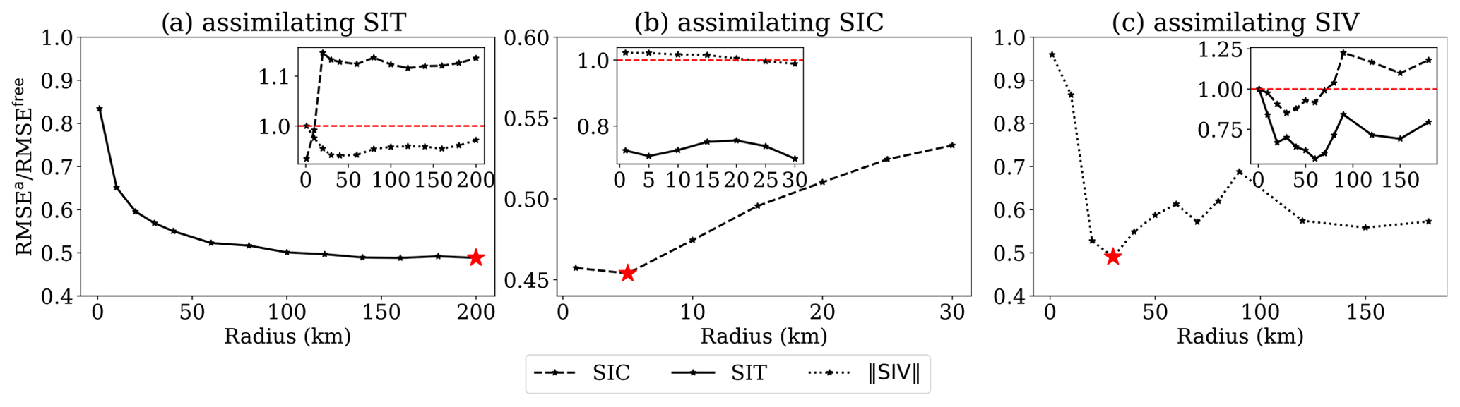
Figure 4 RMSE^a $/$ RMSE^free as a function of the localisation radius, in experiments with observed SIT (a), SIC (b) or SIV (c). The red star indicates the lowest analysis error. The insets show the error in two other unobserved model fields out of the three observed model variables, and the dashed red line indicates the point where RMSE^a = RMSE^free.

The ratio between the root-mean-square error (RMSE) of the analysis and of the free run, as a function of the localisation radius when assimilating SIT, SIC or SIV, is shown in Fig. 4. When assimilating SIT (Fig. 4a), the analysis error in SIT decreases monotonically with the localisation radius until the localisation radius reaches the domain size (200 km). The inset shows that assimilating SIT also leads to a reduction in SIV's RMSE (RMSE^a $/$ RMSE^free systematically below 1), while it leads to a deterioration in SIC as soon as the localisation radius is larger than 5 km.

As opposed to when SIT is observed, the localisation radius for SIC observations (Fig. 4b) is very small. After 5 km, the analysis error in SIC increases monotonically with the localisation radius. Observing SIC improves both SIT and, for very long radii, SIV (see inset in Fig. 4b).

Finally, from Fig. 4c we see that the lowest analysis RMSE when assimilating SIV is attained with a localisation radius of around 30 km and that both SIC and SIT will improve in the multivariate update.

Based on these results, the most effective localisation radii for the observed model fields are 200 km for the SIT observations, 5 km for the SIC observations and 30 km for the SIV observations. These different localisation radii arise from the physical spatial correlations and the observation density of these model fields. A summary of the choices for the localisation radii in this study is given in Table 3, and further discussion will be presented in Sect. 5.1.

4.4 Treatment of bounded physical variables and model parameters

Of the nine MEB model variables, three are bounded: SIC, the level of damage and SIT. Inferring them via the IEnKF is therefore challenging given the Gaussian assumption on which the IEnKF based. In practice, there is no guarantee that the update analyses of SIC, damage level or SIT fall within their bounds.

Hence, the solution to that problem that we adopt in this study, although sub-optimal, is very pragmatic and straightforward. When the analysis of these variables falls outside of their bounds, they are forcibly set to their nearest bounds. We are conscious that this approach leads to local ensemble collapse (whereby some members originally having out-of-range analysis values are all made equal to the nearest boundary value) and can cause biases in the analysis. Nevertheless, the results in Sect. 5 will demonstrate that, when the bounds are not exceeded too often, the approach works well, it does not cause major ensemble collapse and it is successful in removing nonphysical values.

We follow a similar strategy when performing the estimation of the damage parameter, α. There the analysed value of α is assumed to be bounded from below by α=2, the value at which the analysed α will be taken if lower than 2.

Our pragmatic approach is however insufficient when estimating the drag coefficient C_a. This parameter is bounded to be strictly positive; therefore ensemble collapse could happen whenever the ensemble mean of C_a approaches zero. In that case a potentially large number of members may receive negative analysis values that would all be restored to the same small positive values. Hence, we adopt a resampling approach in which, with each negative analysis of C_a, we sample from $\mathcal{N}({\mathrm{10}}^{-\mathrm{5}},{\mathrm{10}}^{-\mathrm{6}})$ until a positive value is obtained.

5 Results

We evaluate the performance of the IEnKF for state and parameter estimation in the dynamics-only MEB sea-ice model under the four different scenarios described in Table 3. We use the root-mean-square error (RMSE) over both time- and space as a skill metric.

5.1 Scenario 1: inferring the model's physical variables under a perfect-model setup

Here we study in detail the fully multivariate DA using different combinations of observations under a perfect-model scenario. The RMSE is calculated over 30 d long assimilation experiments that follow a 42 d free ensemble run without DA. In the 30 d assimilation, we assimilate observations daily as mentioned in Sect. 4.2, leading to a total of 31 analyses.

As mentioned in Sect. 4.4, three out of the nine model fields are bounded quantities: SIC, SIT and the level of damage. Given that respect of those bounds is not automatically guaranteed by the DA procedure, we apply a post-processing step. Here, we quantify how often nonphysical values (i.e. values out of the bounds) are produced in the analysis: Table 6 shows the number of violations during the 30 d DA period.

Table 6 The total percentage of local analyses that violate the physical bounds in the 30 d multivariate DA experiments. “SIC+SIT30+SIV” is an experiment where SIT uses a 30 km localisation radius, whereas “SIC+SIT+SIV” uses a localisation radius of 200 km for SIT.

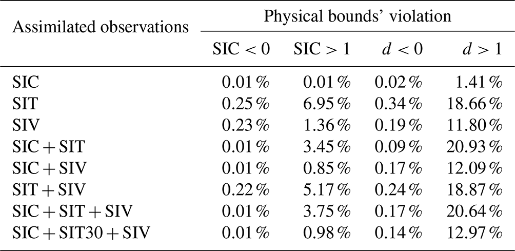
The bound SIT >0 is never violated because SIT is always larger than 1 m in our experiments.

When only SIC is assimilated, physical bounds for SIC and for the level of damage are exceeded very occasionally, for below 1.5 % of the total analyses and grid points. On the other hand, when SIC is not observed, the chance of getting nonphysical SIC analyses increases by 2 orders of magnitude, although it remains below 5.2 %. Similarly, the SIC observations lower the chance of there being nonphysical damage analyses. Notably, when SIT is observed, it leads to analyses that more often violate the physical bounds, particularly the upper bound for the level of damage. The damage bound violations are more severe than those in SIC, since most of the time the sea ice is undamaged and thus very close to the potentially violable bounds of the model fields. Without the possibility of observing the damage field, the cross-correlations may amplify the analysis increments. This effect can be mitigated by limiting the localisation radius of SIT to 30 km as shown in the row of SIC + SIT30 + SIV. The violation of the physical bounds is efficiently addressed by the post-processing step that brings them within their physical limits as described in Sect. 4.4, and it does not lead to an increased RMSE afterwards. As shown in Fig. 5, the SIC analysis is improved compared to the free run in all cases and the sea-ice damage is the only model field that can be less accurate than the free run.

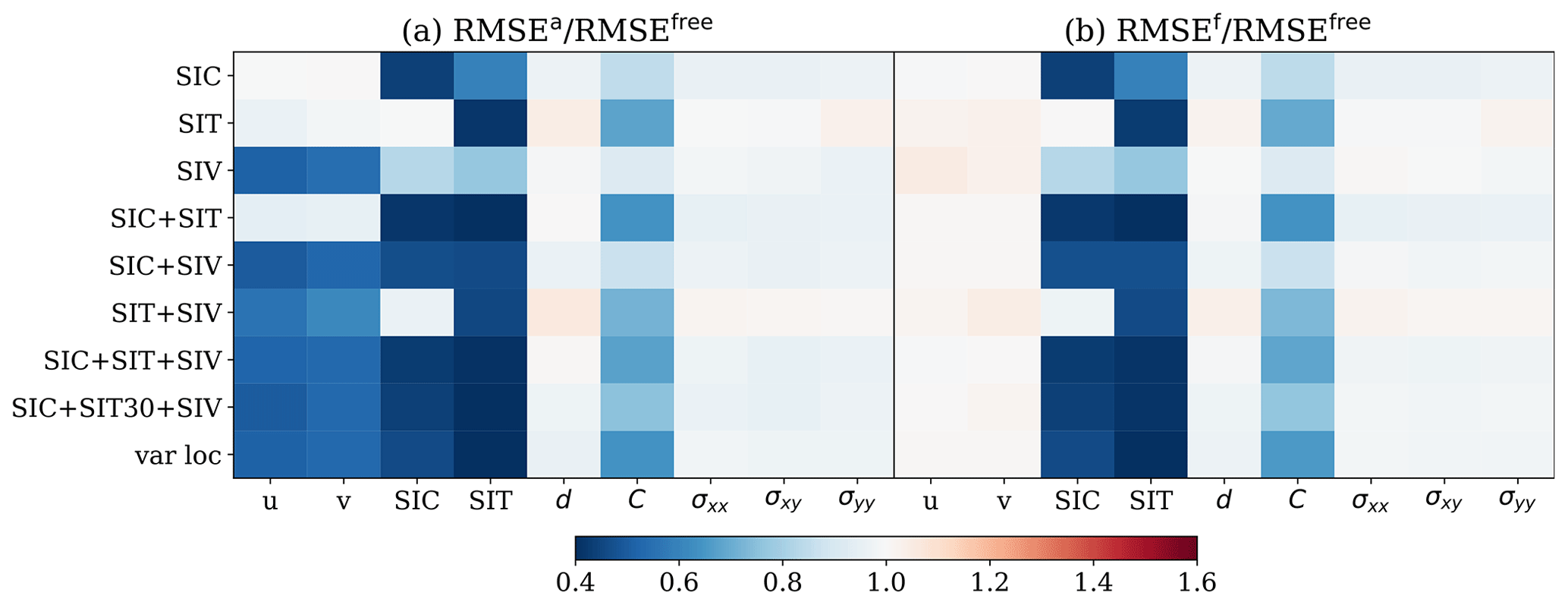
Figure 5 RMSE in the state estimate for scenario 1. (a) RMSE^a $/$ RMSE^free. (b) RMSE^f $/$ RMSE^free. Columns display the individual physical model fields; rows refer to the (combination of) observations that are assimilated.

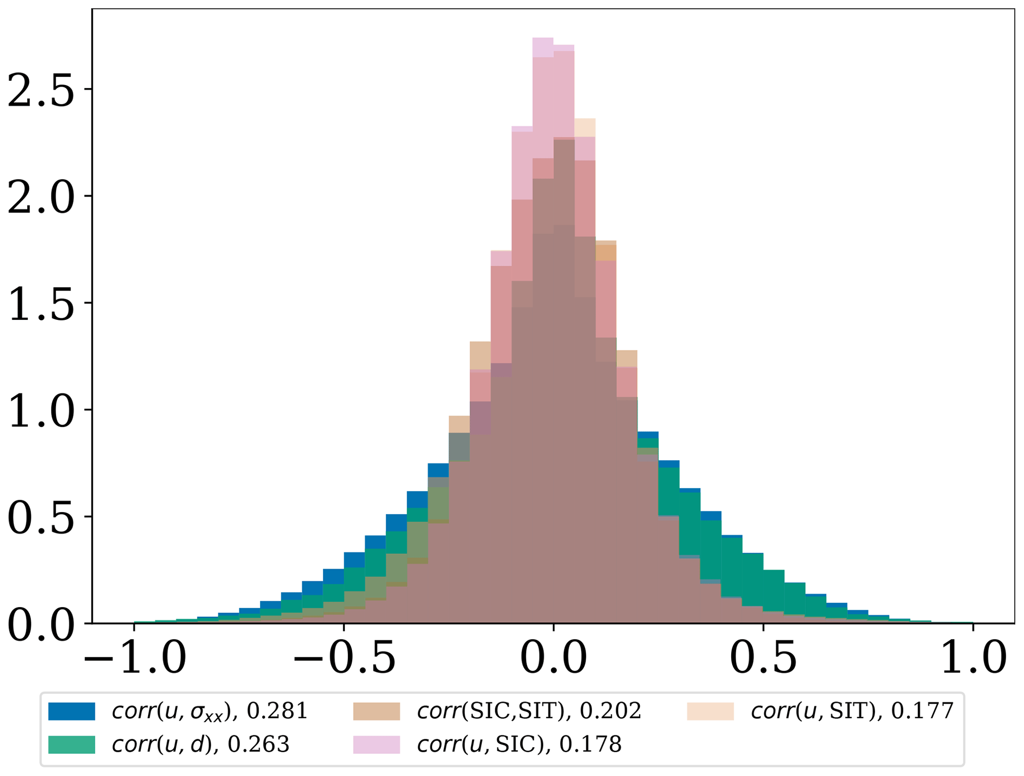
Figure 6 A histogram of the ensemble correlation between model variables when all observations are assimilated over the period of assimilation. The legend indicates the standard deviation of the histogram. A larger spread/standard deviation represents an overall higher correlation between variables.

Figure 5 shows the ratios of analysis $/$ free-run (a) and forecast $/$ free-run (b) RMSE (averaged in space and time) for different types of observations (y axis) and variables (x axis). Values smaller than 1.0 indicate that DA brings about, in general, an improvement in the state estimate compared to the free run. Comparing panels (a) and (b), we can evaluate how much of the DA update is effective in reducing the forecast error (recall that the analysis cycle is 1 d long). From the figure we immediately notice that when only one observation field is assimilated, that same field is the area where most of the improvement in the analysis occurs. This is consistent with our results in Sect. 4.3.2. Figure 5 also shows almost no changes/slight improvements in SIV analysis when SIC alone is assimilated and conversely for the SIC analysis when SIT is assimilated. This appears to be in contrast to Fig. 4, which indicates that SIT observations have a negative impact on the SIC analysis and that SIC observations can cause SIV analysis to deteriorate at certain localisation radii (see Fig. 4a and b insets). Nevertheless, the longer experiments of Fig. 5 suggest that the ensemble has acquired dynamical consistency and therefore better reproduces the cross-variable correlations.

In the MEB rheology, the level of damage, cohesion and stress have a close relationship. Without assimilating SIT, the IEnKF-N leads to improvements in sea-ice cohesion and stress and some improvements in the level of damage too. However, the assimilation of SIT tends to result in overly damaged sea ice. This is also evident from Table 6, where it can be seen that the assimilation of SIT leads to higher chances of breaking the bounds of the level of damage. This adverse effect on the damage and stress persists when SIT is assimilated together with SIV. Interestingly, however, when SIT is assimilated together with SIC, the boundedness of the level of damage is improved for undamaged sea ice (d<0) but is not for completely damaged sea ice (d>1). However, it is sufficient to improve the overall RMSE of the level of damage (see Fig. 5). One possible reason for this is that, without the thermodynamics, the forecast error mainly comes from the damaged sea ice and the overestimation of undamaged sea ice makes little contribution to the RMSE after the post-processing. An ad hoc remedy is to use a shorter localisation radius for SIT (experiment SIC + SIT30 + SIV in Fig. 5), although it also reduces the improvements in SIT and cohesion. Moreover, as a result of better cross-correlations, the use of small localisation mitigates the violations of physical bounds, as shown in Table 6. Another approach to avoiding the negative impact of SIT consists in artificially setting the covariance matrix entries between SIT and SIC and between SIT and damage to zero. This is achieved in practice by assimilating only SIC and SIV for the SIT and damage variables while all observations are assimilated for the rest of the state vector. The experiment “var loc” shows improved results in Fig. 5.

We show the strength of the cross-correlations between different model variables in Fig. 6. The values are taken from the experiment where all observations are assimilated, from all spatial points and all analyses. As expected, the distributions all peak around zero: this is because beyond a certain distance, the correlations are all very small (a fact that is at the basis of the use of localisation), with the larger values concentrated in proximity to the analysis point and populating mainly the tails of the distributions in Fig. 6. The width of the distributions indicates that in many instances the correlations are (in absolute values) as high as 0.5. To provide a quantitative comparison among the distributions' width, we also show the standard deviations. These cross-correlations can be understood from a physical point of view. The cross-correlations between SIV and stress are the strongest as SIV is mainly driven by the external wind field. In addition, SIV, stress and the level of damage are closely coupled processes, so the level of damage and SIV also show strong cross-correlation. The weak cross-correlation between SIV and SIC and between SIV and SIT is a result of the small magnitude of SIV, which transports SIC, SIT and cohesion. Nevertheless, this gives rise to a strong correlation between SIC and SIT because they are both controlled by the advection processes.

A physical interpretation can also be invoked to explain why the improvements in SIV analysis do not necessarily translate into improvements in the forecast, as shown in Fig. 5. We argue that this is due to the instant injection of error from the wind field after the assimilation of observations. The correction from the assimilation acts as a perturbation to the model, which induces a model adjustment. In contrast to SIV, the increased error in the analysis of the level of damage, when assimilating SIT, is mitigated by the further damage caused by the wind field. On the other hand, the longer timescale of the variability in SIC, SIT and cohesion makes them less sensitive to the model adjustments, and thus better analysis generally yields better sea-ice forecasts (see Fig. 5).

In summary, our experiments show that the IEnKF can improve both the analysis and the forecast of the MEB sea-ice model. We confirm, in line with previous studies, the necessity of controlling the main source of the uncertainty from the external forcing in the sea-ice model. We argue that a correct wind field can counteract the deterioration of the inaccurate SIV forecast. Furthermore, the results also demonstrate the positive impact of a variable-dependent localisation radius in combating both sampling error and nonlinearities. Moreover, even if the IEnKF suffers from sampling error with a large localisation radius, the deterioration of some of the unobserved fields is marginal, with the RMSE being only 6 % larger than the free run. With a reduced localisation radius, the IEnKF improves all the unobserved fields.

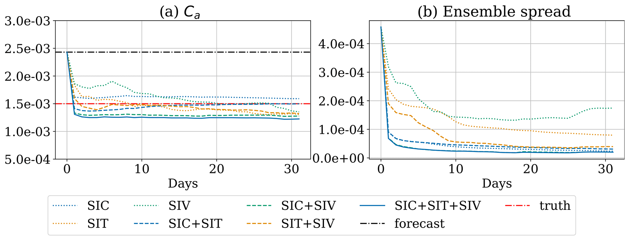
Figure 7 Time series of (a) the analysis of C_a using different combinations of observations and (b) the analysis ensemble spread of C_a.

5.2 Scenario 2: inferring the model's physical variables and the drag coefficient C_a

We achieved satisfactory performance in the state estimation of the MEB model using the IEnKF-N under the perfect-model assumption. In the experiments described in this section, we assume that C_a is incorrectly specified and attempt to recover the true value using DA, while all other parameters are perfectly known.

The air drag coefficient, C_a, controls the degree to which momentum from the wind is transferred to the sea-ice cover. In our model, similarly to most sea-ice models, it is a constant scalar value that modulates the wind drag; see Eq. (2). Equation (2) shows two main sources of uncertainties in the same term: the wind field, u_a, and the drag coefficient, C_a. The multiplicative role of C_a makes it an amplification factor for the uncertainty that originates from uncertain wind fields. Given that the wind field is the main source of uncertainties in the sea-ice dynamics, the incorrect specification of C_a also affects the predictability of the sea ice. To see this, note the larger free-run ensemble spread in this scenario compared to the perfect-model scenario in Table 5. Note that the difference in the C_a between scenarios 1 and 2 is as small as 10⁻³ (see Table 3).

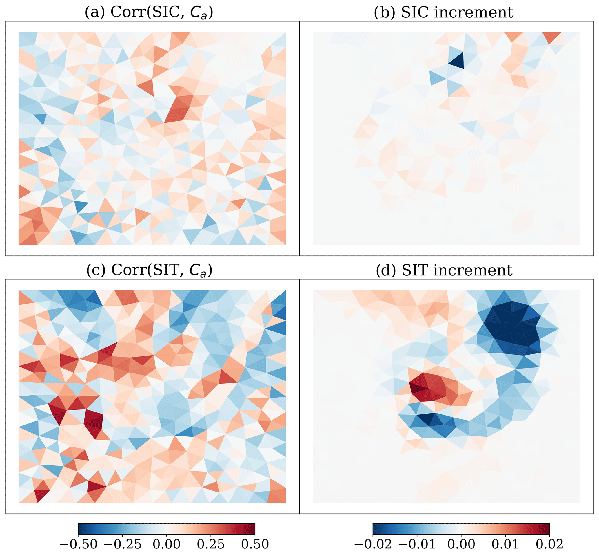
Figure 8 Cross-correlation between the observation and C_a: (a) correlation between SIC and C_a at the last analysis; (b) SIC increment. In both cases it refers to the experiment where only SIC is assimilated; panels (c) and (d) are the same as panels (a) and (b) but with SIT in place of SIC in the experiment where only SIT is assimilated.

Similarly to the state estimation experiments, the assimilation starts after a 42 d free ensemble run. Figure 7a shows the time series of the analysis of C_a, while Fig. 7b shows the analysis spread in C_a as a function of time. We see that after the drastic correction of the initial bias, the ensemble spread stabilises for all experiments. The ensemble spread converges and stabilises to slightly above zero except for the case where only SIT/SIV is assimilated. In those cases, the ensemble spread is larger, which might be a consequence of the sparser observation density. Due to SIV being sensitive to C_a, the estimation of C_a is affected by changes in SIV observations. These changes are captured by the adaptive inflation scheme leading to an increased ensemble spread of C_a toward the end of the experiment period. Another remarkable feature is that in all experiments, C_a drops significantly over the first time steps, thereby approaching (but not necessarily converging to) the true value (red line). This is a clear consequence of a strong correlation between the observed fields and the parameter. Besides this, we then observe different converging values and performance depending on the type of observations assimilated. Except for the case where only SIC is assimilated, the analyses underestimate C_a at the end of our experiment time. The smaller increments of C_a, when assimilating SIC, are a result of smaller cross-correlation between SIC and C_a in comparison to SIT and C_a as shown in Fig. 8a and c. Similarly to the increments of C_a, the SIT experiment also shows increased increments of the observed fields compared to the SIC observation, as in Fig. 8b and d. This suggests that the ensemble spread in SIT is larger than in SIC. Moreover, the cross-correlation of the ensemble anomaly between SIC/SIT and C_a is spatially inhomogeneous (see Fig. 7a and c). This implies that the error is controlled not solely by the global parameter but also by other spatially dependent processes. One possible explanation is the error in the wind fields. As the ensemble error is primarily driven by the error in the wind field scaled by C_a acting as wind forcing, the cross-correlation between the C_a and the observations may be affected by the error in the wind fields. This suggests that while the IEnKF successfully corrects large biases in C_a, it may not be able to correct errors of smaller magnitude equally well as the errors can be aliased with the error in the wind field. In the latter case, the estimation of C_a does not necessarily converge to the “true” C_a.

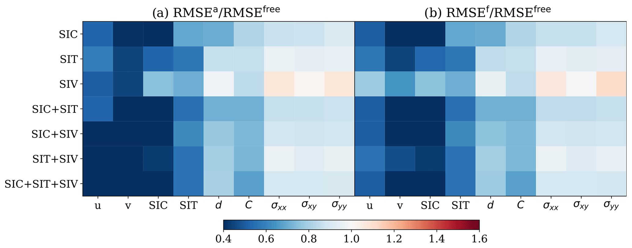
Figure 9 RMSE in the state estimate for scenario 2. (a) RMSE^a $/$ RMSE^free. (b) RMSE^f $/$ RMSE^free. Columns display the individual physical model fields; rows refer to the (combination of) observations that are assimilated.

The correction of C_a is also effective in the state estimation as shown in Fig. 9. The IEnKF efficiently controls the RMSE for nearly all model fields regardless of the combination of observations compared to the free run that is instead affected by a large bias in C_a. Notably, compared to the free run, SIV is improved not only in the analysis, but also in the forecast. This is different from the multivariate update in Sect. 5.1 because the positively biased C_a amplifies the uncertainties from the wind field, which is then reduced by the corrected C_a. The time series in Fig. 10c–d show that the corrected C_a significantly reduces the bias in SIV, but the transient error in the wind forcing still impacts the accuracy of the SIV forecast.

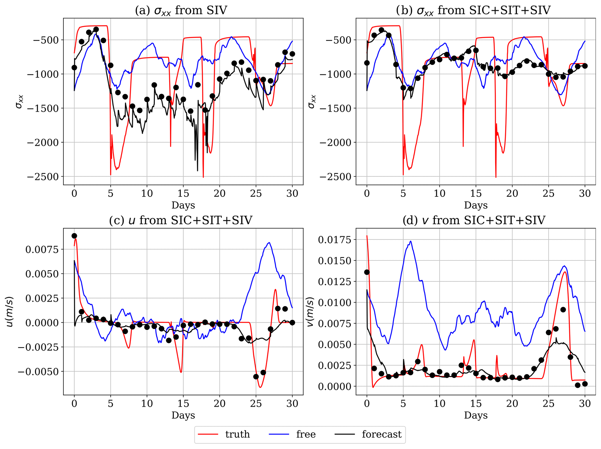
Figure 10 Time series of (a) sea-ice stress in the x direction when only SIV is assimilated, (b) sea-ice stress in the x direction when all observed fields are assimilated, and SIV in the (c) u and (d) v component when all observed fields are assimilated. The black points in the time series are the spatially averaged analysis.

In Fig. 7a, the best skill in estimating C_a is achieved when assimilating SIC alone due to its higher observation density. However, even with fewer observations, SIV achieves good performance due to a close relationship with the wind field and C_a in Eq. (2). Notably, assimilating only SIV greatly reduces the RMSE across all model fields except for the sea-ice stress (see the third row in Fig. 9a). The increased RMSE in the sea-ice stress arises because the DA update of the stress sometimes severely violates the constitutive equation. This can potentially lead to unstable model solutions and model crashes. Model crashes can be avoided by using a large number of iterations for the MEB solver during an extended period after the DA step, but the unphysical update still leads to inaccurate forecasts of the sea-ice stress (see the third row in Fig. 9a). The inaccurate stress forecast can be observed in Fig. 10a, which shows a significant underestimation in the stress time series around day 17. Such underestimation does not occur when all observations are assimilated, as shown in Fig. 10b. We found that the erroneous stress underestimation in the time series occurs when the local element of SIC is reduced by the assimilation (not shown) to the point that it creates a large SIC gradient and increases the elastic behaviour of the sea ice (see the right-hand side of Eq. 3). Since the temporal variation in SIC is small, this issue persists, and a continued decrease in the sea-ice stress along with the model integration is maintained. This incorrect SIC estimate is remedied in the next DA step, where the multivariate DA restores SIC. Hence, assimilating SIC mitigates the unphysical DA update. Arguably, it is unlikely that only SIV is assimilated in real scenarios, yet our results suggest that it is wise to restrict the multivariate update of the sea-ice concentration in this case.

Our experiments show that the IEnKF is able to reduce the bias in C_a based on available sea-ice observations. The improved C_a estimation significantly reduces the error in the model fields. From the momentum equation, Eq. (2), we know that SIV is directly linked to C_a. However, our results show that, although assimilating SIV is crucial for estimating C_a, SIC and SIT still improve the estimate of C_a and the state. Importantly, when assimilated in conjunction with SIV, SIC and/or SIT mitigates the imbalance of the constitutive equations.

Figure 11 Time series of (a) the analysis of α and (b) its ensemble spread.

5.3 Scenario 3: inferring the model's physical variables and its erroneous damage parameter α

While the drag coefficient, C_a, is linked to the external forcing, the internal property of the sea ice is largely controlled by the damage parameter α. The damage enters the model in the stress equation, Eq. (3). Although α is added to the model in an ad hoc manner, it plays an essential role in the MEB rheology as it sets the rate at which viscosity decreases with increasing level of damage and thereby controls the transition between the elasto-brittle regime at low damage levels and the viscous regime at high damage levels.

Model sensitivity studies by Dansereau (2016) and Weiss and Dansereau (2017) showed that the value of α is critical in determining the macroscopic mechanical behaviour of the model and that a value of α≥4 leads to complex, sea-ice-compatible, behaviours. In fact, in our experiments, the truth, i.e. the un-biased model, is set to α=4 (see Table 3). In the DA experiments with the estimate of α, we mimic an initial biased estimation of the parameter that is in the same range of sea-ice-compatible behaviour: we choose α=6.5 (see Table 3). Our strategy is realistic as the initial “guess” does not cause the model to behave qualitatively differently from the observations when α≥4. Drastic changes in the dynamical regimes are also challenging for DA, and they influence the error dynamics between the model parameter and the observed fields. Given that the IEnKF updates (in both the state fields and the parameters) are unbounded, we apply the same post-processing to keep the analyses within physically acceptable bounds, as described in Sect. 4.4.

One of the fundamental challenges in estimating α arises from the nonlinear relationship between α and the observed fields. In particular, the parameter is directly related to the stress field, which is not observable. The complex, nonlinear and indirect nature of these relations can lead to inaccurate (finite-)ensemble-based cross-correlations. Another potential challenge comes from the low sensitivity of the model fields to α compared to the wind field and C_a (see Fig. 1). As shown in Table 5, in a 90 d free run, the ensemble spread of observed model fields is only marginally larger than that in the perfect-model scenario.

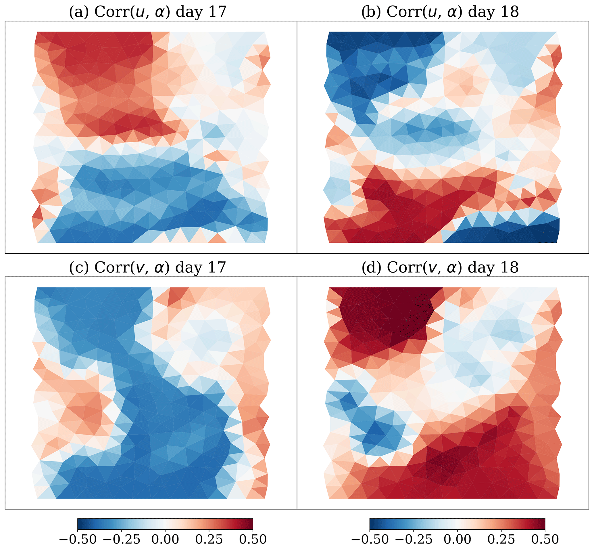
Figure 12 Cross-correlation between the (a, b) u and (c, d) v component of SIV and α on day 17 and 18 when only SIV is assimilated.

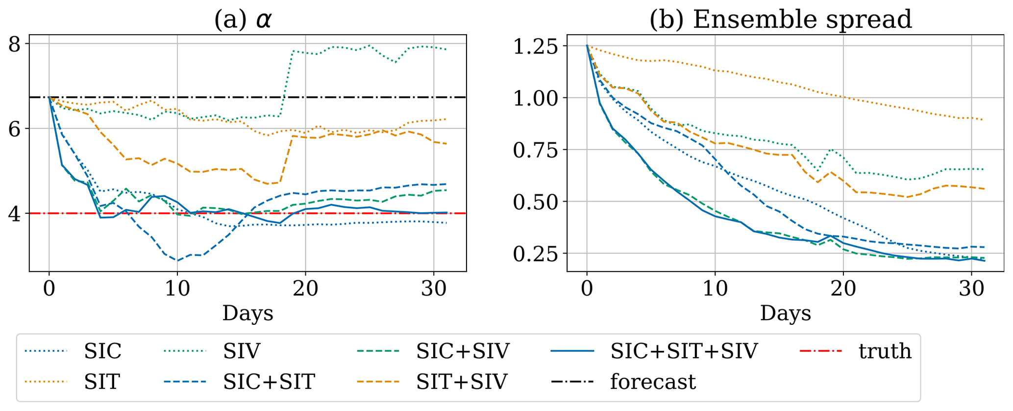
Despite these obstacles, the IEnKF shows encouraging results in estimating α, as shown in Fig. 11a. Assimilating SIC or SIT alone leads to under- and overestimation of α after 30 d. From Fig. 11b, we see that the ensemble spread in SIT is still relatively large at the end of the experiment. This suggests not only that it is only slightly reduced at the analysis steps but also that further adjustment of α beyond the 30th day is still a possibility. The simultaneous assimilation of SIT and SIC leads to a good approximation of the true value of α=4. Similar results are attained whenever SIC is assimilated (see experiment SIC + SIV or SIC + SIT + SIV). This suggests the crucial relationship between α and SIC, which appears to be the key observation for inferring the damage parameter.

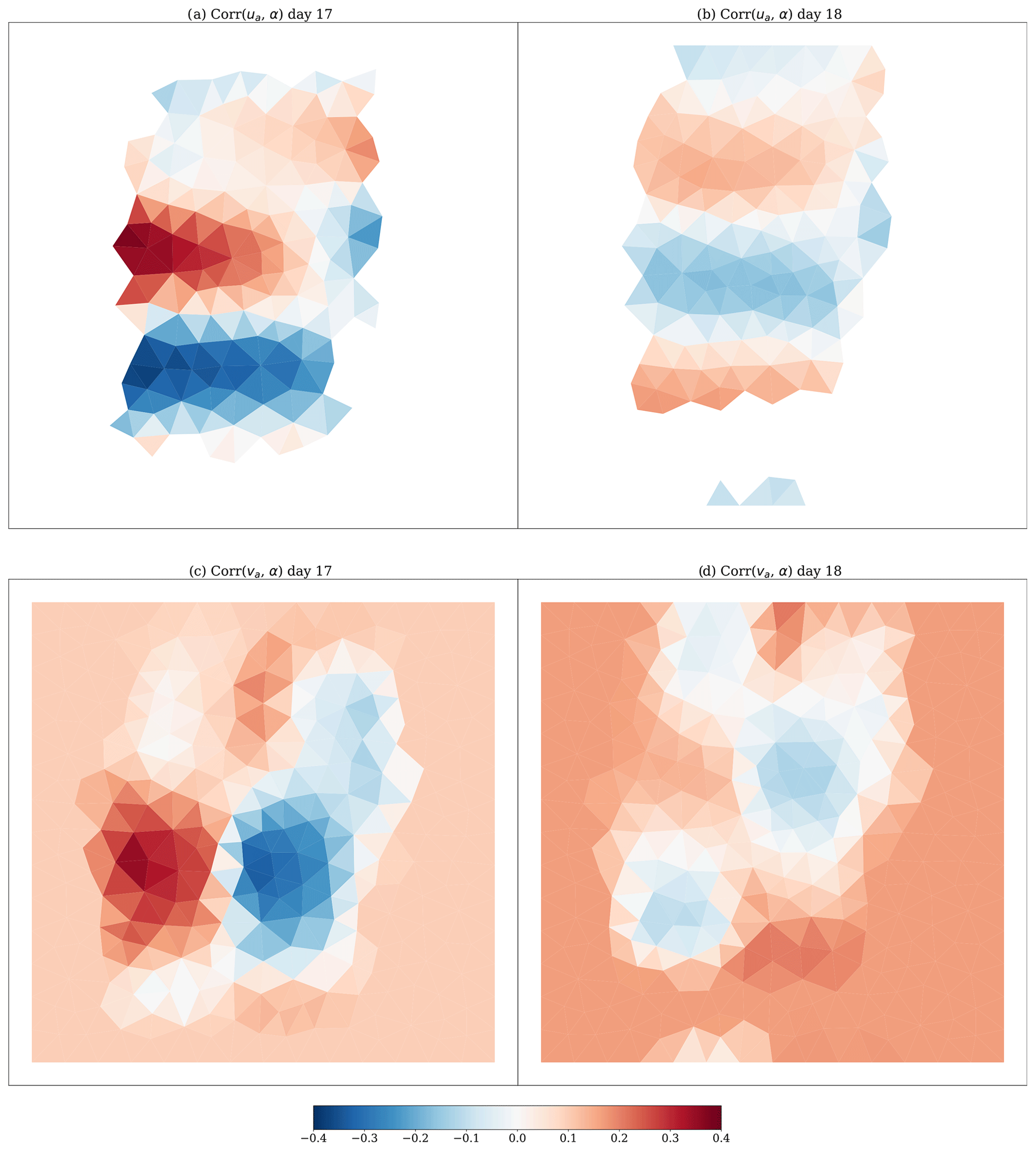
Figure 13 Same as Fig. 12 but for the components of the wind forcing in place of those of SIV.

Our results also suggest that observations of SIV cannot be used to retrieve α effectively. In all the experiments with SIV observations, the estimated α gradually approaches the truth until day 18, when it then abruptly diverges away from it. An insight into the reasons behind this sudden change is provided in Fig. 12, which shows the spatial distribution (on the model domain) of the cross-correlation between α and either u or v, on days 17 and 18. The cross-correlations between SIV and α flip their signs spatially from day 17 to 18. This is related to the uncertainties in the wind field, which dominate the forecast uncertainty in SIV.

Let us illustrate this issue with simple mathematical arguments. We assume that the nonlinear sea-ice model, ℳ, can be approximated by its linearisation M within the forecast interval between two successive analyses. The forecast ensemble anomaly (error) of SIV at time step k can be approximated as

$$\begin{array}{}\text{(7)}& \mathit{\delta }{\mathbf{u}}_k={\mathbf{M}}_k^{\mathit{\alpha }}\mathit{\delta }{\mathit{\alpha }}_{k-\mathrm{1}}+{\mathbf{M}}_k^{u_{\mathrm{a}}}\mathit{\delta }{{\mathbf{u}}_{\mathrm{a}}}_{k-\mathrm{1}}+{\mathbf{M}}_k^x\mathit{\delta }{\mathbf{x}}_{k-\mathrm{1}}+\mathcal{O}\left(\mathrm{2}\right),\end{array}$$

where δ⋅ represents the deviation from the ensemble mean and x is the state vector except the damage parameter; the superscript means the model sensitivity to the corresponding variables in which ${\mathbf{M}}_k^{\mathit{\alpha }}\in {\mathbb{R}}^{n\times \mathrm{1}}$, ${\mathbf{M}}_k^{u_{\mathrm{a}}}\in {\mathbb{R}}^{n\times m}$ and ${\mathbf{M}}_k^x\in {\mathbb{R}}^{n\times l}$, with n being the number of SIV values in the controlled vector, m being the number of elements in the wind field vector and l being the number of elements of model state in the controlled vector. 𝒪(2) represents the high-order terms that are greater than second order. In the EnKF (and thus in the IEnKF), the cross-covariance is estimated from the ensemble anomaly of SIV and the perturbations of α, which approximate $\mathbb{E}\left[\mathit{\delta }{\mathbf{u}}_k^T\mathit{\delta }{\mathit{\alpha }}_k\right]$. This cross-covariance between SIV and α is related to the perturbation (error) from the model state, wind and α. In our case, whenever $\left|\right|{\mathbf{M}}_k^{u_{\mathrm{a}}}\mathit{\delta }{\mathbf{u}}_{\mathrm{a}}\gg {\mathbf{M}}_k^{\mathit{\alpha }}\mathit{\delta }\mathit{\alpha }\left|\right|$, the SIV uncertainty is mainly driven by the wind. This can falsely give a strong cross-correlation between SIV and α, producing an incorrect α estimate when it is only based on SIV observations. A similar issue was encountered in Simon and Bertino (2012), where the authors found the parameter estimation challenging when the uncertainty in the parameters showed relatively low uncertainties in the observed fields.

Based on this argument, we can show that the sign flip of cross-correlations in Fig. 12 is a result of the change in wind field. In Fig. 13, the cross-correlation between the wind field and α shows the periodic northward travel of the storm on the y axis (see Fig. 13a and b) and the rotation of the storm (see Fig. 13c and d). This matches the changes in cross-correlations in Fig. 12. The incorrect estimate of α highlights the challenges when the primary sources of the uncertainties are external instead of being the model parameters. We observe that this effect also influences the α estimate when SIV is assimilated with the SIT.

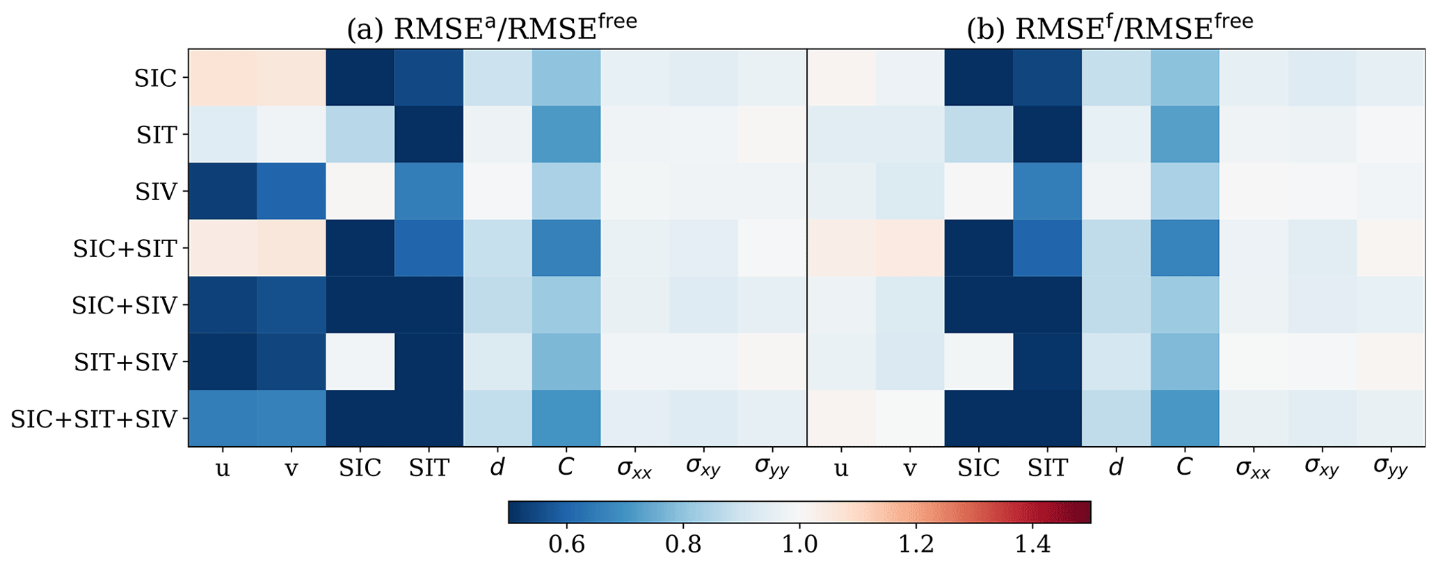
Figure 14 RMSE in the state estimate for scenario 3. (a) RMSE^a $/$ RMSE^free. (b) RMSE^f $/$ RMSE^free. Columns display the individual physical model fields; rows refer to the (combination of) observations that are assimilated.

Figure 14 shows the improvements in the state estimate. As expected, the analyses of the observed fields are in general more accurate than the free run. Moreover, compared to the perfect-model scenario, the damage field is now improved relative to the free run in all experiments. The stress field is only moderately improved even though it has a direct relationship with α in Eq. (3).

Interestingly, without observing SIV, the assimilation of SIC shows a negative impact on the analysis of SIV. This may be a result of the underestimated α in these experiments. With a low value of α, the sea ice has a more elastic behaviour. The elastic motion has a short timescale and is sensitive to the perturbation of the sea-ice variables, making the slowly changed SIC observations unreliable. This is consistent with the finding from Weiss and Dansereau (2017) such that, with high α values and the sea ice transitioned from elastic to viscous behaviour, the system becomes more predictable. When SIV is assimilated, the overestimated α leads to only slight error increases in the SIC analysis without hampering the state estimation of other model variables. This suggests that the model state and parameter are adjusted based on the primary source of error, the wind forcing.

Our results demonstrate the possibility of estimating α successfully using as many as possible of the available observations. It is notable that no single type of observation alone can infer α accurately. We also demonstrate that the IEnKF cannot always identify the correct source of error in a complex environment. In our case, the error from the wind field negatively impacts the estimation of α. Interestingly, a deteriorated α analysis does not necessarily lead to a deteriorated state estimation. In contrast, the overestimation of α still moderately improves the sea-ice forecast due to improved predictability.

5.4 Scenario 4: inferring the model's physical variables and its erroneous C_a and α

In the previous sections we demonstrated that, with sufficient observations, the IEnKF can estimate C_a and α when only one of them is erroneous. Considering that both C_a and α are in the closely related equations for SIV and stress (see Eqs. 2 and 3), it is of interest to investigate the possibility of estimating both model parameters simultaneously.

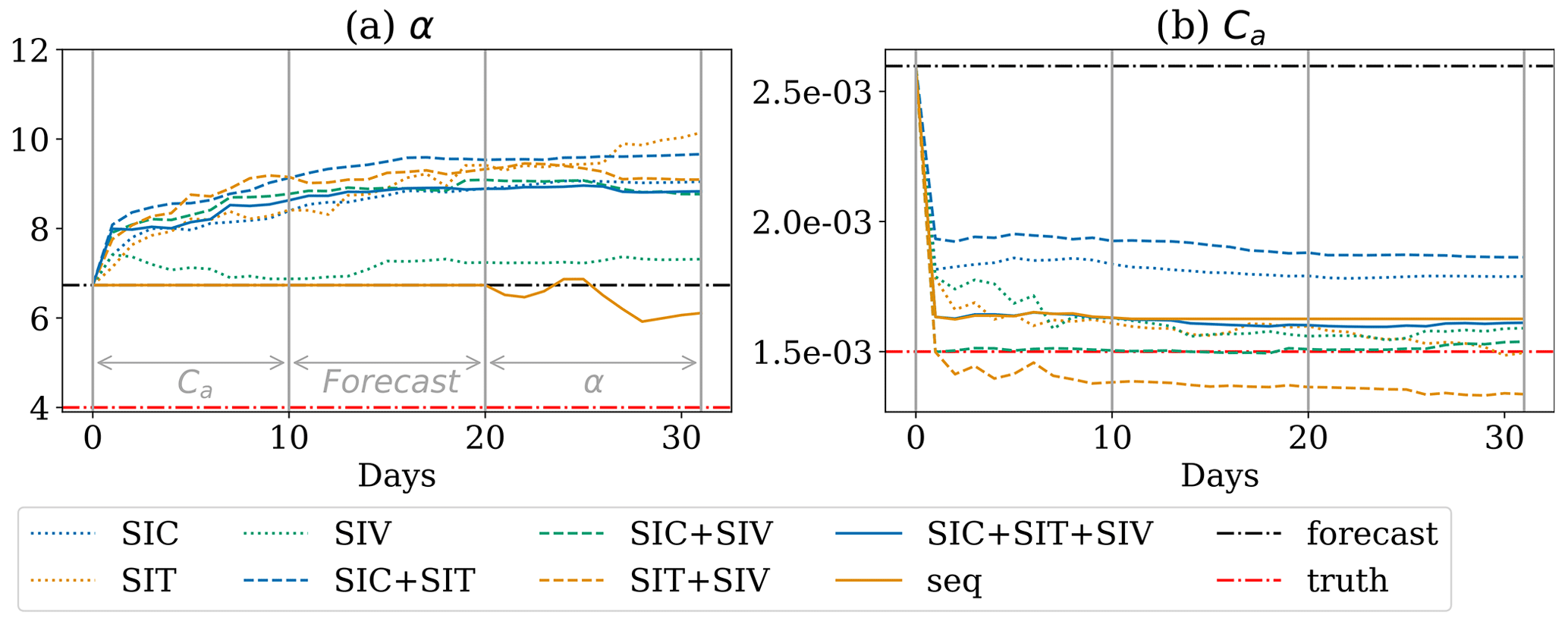
Figure 15 The analysis of the α (a) and C_a (b) parameter estimate based on a variety of combinations of observations.

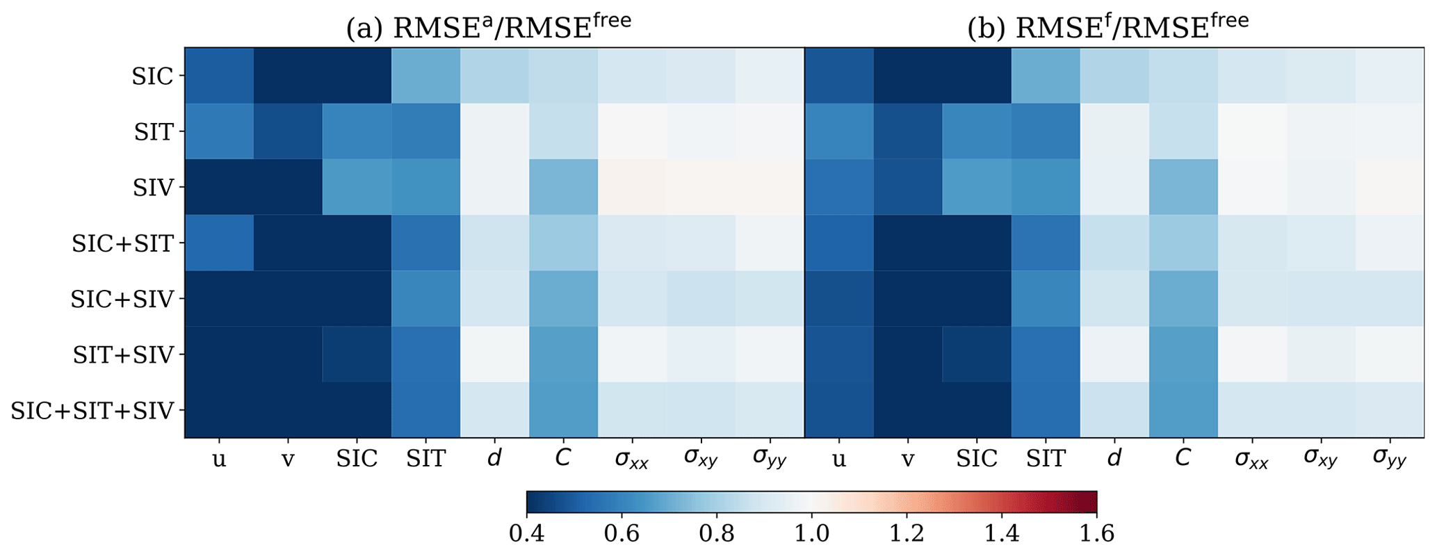
Figure 16 RMSE in the state estimate for scenario 4. (a) RMSE^a $/$ RMSE^free. (b) RMSE^f $/$ RMSE^free. Columns display the individual physical model fields; rows refer to the (combination of) observations that are assimilated.

Figure 15b shows the estimated C_a after 30 d of assimilation. All experiments approach the true value of C_a (although starting from an overestimated value). When SIC and SIV are assimilated together, the IEnKF gives the best estimate of C_a, while it underestimates C_a when only SIT and SIV are assimilated. The IEnKF also gives an increase in the estimate of α as shown in Fig. 15a. Although this demonstrates the difficulty in estimating both parameters, it is remarkable that it still leads to an improved forecast of model fields as shown in Fig. 16. This is known as a compensating effect (Bocquet, 2012). This apparent contradiction is related to the non-identifiability of the problem whereby the parameter estimation cannot fully reconstruct the true parameters. In practice, this implies that more than one set of parameters can produce the same observed fields. The identifiability issue can also be viewed from a physical standpoint: C_a determines the motion of the sea ice via the wind forcing. With overestimated a priori C_a, the wind can cause fast sea-ice motions. α influences the rate at which sea ice transitions from an elasto-brittle solid behaviour to a viscous fluid behaviour with an increasing level of damage. As discussed in Sect. 5.3, the increased α leads to more viscous sea ice that is more easily subjected to permanent deformations instead of fast transient elastic deformations. In this situation, the IEnKF controls the fast sea-ice motions by removing the elastic sea-ice deformations.

The identifiability issue can also be associated with incorrect cross-correlations between model fields and model parameters from different sources of errors as described in Eq. (7). We observe that assimilation correctly decreases C_a, showing a relatively accurate cross-correlation between the observations and C_a. This controls the impact of the external wind forcing, as a positively biased C_a can amplify the uncertainty in the wind field, which increases the term ${\mathbf{M}}^{u_{\mathrm{a}}}\mathit{\delta }{\mathbf{u}}_{\mathrm{a}}$ in Eq. (7). As discussed in Sect. 5.3, the outstanding external wind forcing could lead to erroneous estimation of α. Hence, after the external uncertainties are controlled, the ensemble should be able to develop reasonable cross-correlations between α and the observations. To test this, we adopt the following strategy in the 30 d assimilation experiments: (1) constraining the external uncertainty by estimating C_a only for 10 d, (2) developing uncertainty from α by model forecasting without assimilation for 10 d and (3) estimating α for the last 10 d. This is labelled “seq” in Fig. 15. Although C_a is still underestimated, we observe a reduction of error in α. Also, as other experiments do not show a decreased α after an underestimated C_a, this may suggest the importance of step (2), where the uncertainty arising from α developed. We stress here that the 10 d is simply chosen for convenience and is not tuned.

To further consolidate our findings on the performance of the IEnKF in the simultaneous parameter estimations of C_a and α, extensive, and computationally demanding, investigations with different model states, forcings and parameters would be ideal. In fact, even though the model is a simplification of a full pan-Arctic sea-ice model, the computational power quickly scales up to beyond our resources.

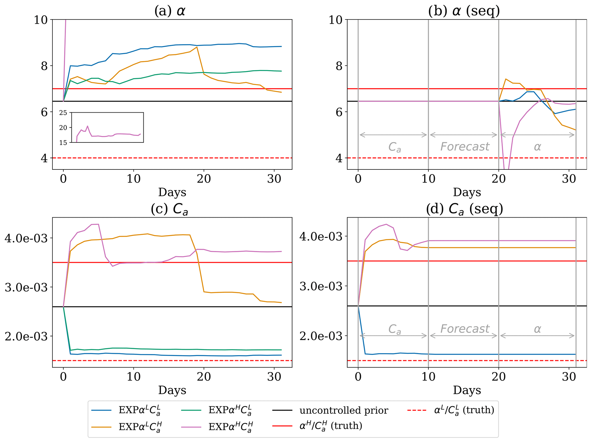
Figure 17 Simultaneous parameter estimation of C_a and α with different sets of truths of these parameters. The horizontal red lines represent the truth values when they are either lower or higher than the initial guess. The inset in (a) is the estimated α in the experiment EXP${\mathit{\alpha }}^H{C}_{\mathrm{a}}^H$.

With the aforementioned computational constraints in mind, we performed three additional experiments using different truths. In addition to the existing experiment (EXP${\mathit{\alpha }}^L{C}_{\mathrm{a}}^L$) where we assimilate all observations to estimate α and C_a, we implemented three other experiments where the truth uses (1) α=4 and $C_{\mathrm{a}}=\mathrm{3.5}\times {\mathrm{10}}^{-\mathrm{3}}$ (EXP${\mathit{\alpha }}^L{C}_{\mathrm{a}}^H$), (2) α=7 and $C_{\mathrm{a}}=\mathrm{1.5}\times {\mathrm{10}}^{-\mathrm{3}}$ (EXP${\mathit{\alpha }}^H{C}_{\mathrm{a}}^L$), and (3) α=7 and $C_{\mathrm{a}}=\mathrm{3.5}\times {\mathrm{10}}^{-\mathrm{3}}$ (EXP${\mathit{\alpha }}^H{C}_{\mathrm{a}}^H$). Here, the superscript L and H denote that the truth is lower and higher respectively than the initial guess. We investigate relevant scenarios (e.g. under- or overestimation of the real values) in which the model's qualitative behaviour is of the same sort. The latter specifically concerns the model structural stability, that is to say the fact that the model is not subject to bifurcation of its general behaviour.

When the truth of model parameters is higher than the initial guess, the air drag coefficient is 2σ above the initial guess while α is 1σ above the initial guess. Keeping the value up to 1σ higher than the initial guess of α is due to the changes in the dynamical regime of the model that occur beyond 1σ. As discussed in Dansereau (2016), when α increases, the sea ice loses memory of the previous damage events, leading to increasing elasto-plastic behaviour. This implies that a different set of initial guesses might be needed for these dynamical regimes as we do not expect that the IEnKF to be able to provide reliable estimation when a change in dynamical regime occurs. Meanwhile, based on physical arguments, such a high α parameter is less likely to occur in reality where the true value is likely to be between 4 and 7. As shown in Fig. 17, EXP${\mathit{\alpha }}^H{C}_{\mathrm{a}}^L$ gives improvements in the air drag coefficient, and, though overestimated, the α parameter is increased as prescribed by the truth. In EXP${\mathit{\alpha }}^L{C}_{\mathrm{a}}^H$, improved C_a estimation is obtained at the start of the estimation but deteriorates after 20 d. In EXP${\mathit{\alpha }}^H{C}_{\mathrm{a}}^H$, though the C_a parameter is improved, the estimation of α is approximately 17, which is 1 order of magnitude larger than the truth. The deteriorated results occur when the true C_a is higher than the initial guess, which corresponds to a strong wind forcing in the truth. One possible explanation for this is that the correlations between α and the observed fields are not truthfully reflected due to the strong wind forcing. Nevertheless, if we first estimate the air drag coefficient, followed by a free forecast phase, and estimate α afterwards, the parameter estimation is improved. This shows that even if the same prior distribution is used, different dynamical regimes of the modelled truth can lead to different results in the experiments.

Our results suggest that the augmented state vector can have identifiability issues when both C_a and α are biased. As shown in Table 5, the perturbation of α cannot provide greater forecast uncertainty compared to the positively biased C_a. We have proposed a strategy to overcome the issue with some discussions on alternative approaches. For example, a larger ensemble spread of α may increase the uncertainty in the forecast ensemble, which avoids a single dominant source of forecast uncertainty. We note that, based on our reasoning, the identifiability issue may not exist when C_a is negatively biased. Nevertheless, this demonstrates a potential issue with the parameter estimation in MEB-type sea-ice models.

5.5 Impact of parameter estimation on long-term prediction

It is worth studying the impact of the parameter estimation on the long-term performance of the model. To this end, we performed a 90 d long free run whereby the model parameters are “frozen” to the values obtained at the end of the DA period. The experiment is carried out for the case when both C_a and α are estimated during the DA period using the configuration “seq” of Sect. 5.4. Results are displayed in Fig. 18.

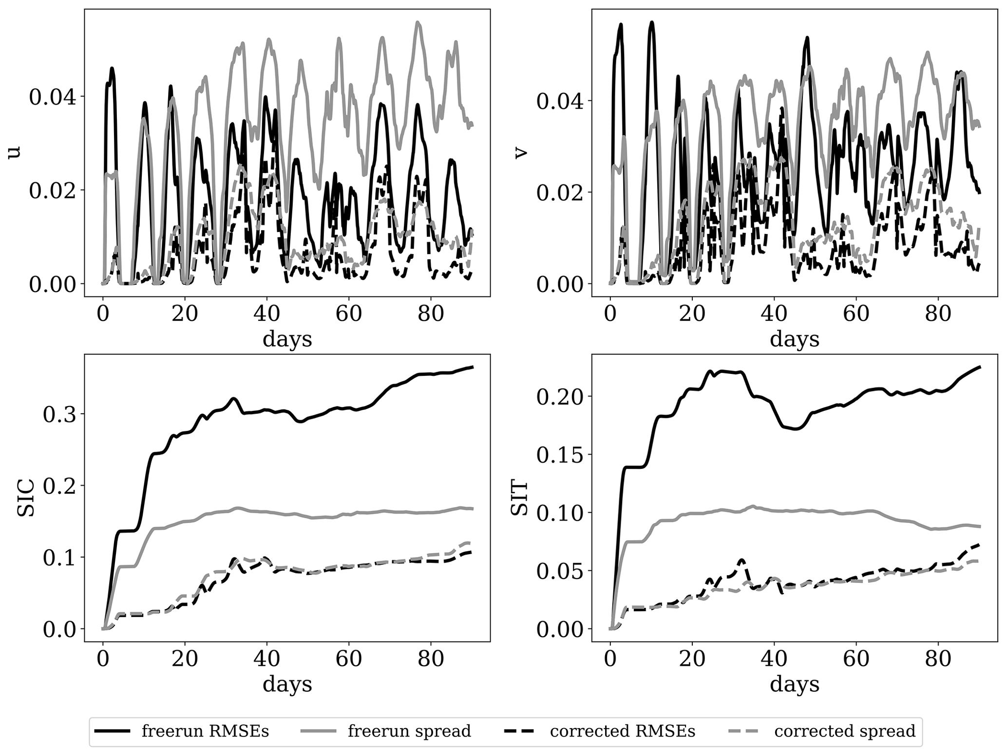
Figure 18 RMSE and ensemble spread of the free run using prior parameters and parameters corrected by the DA when both C_a and α are erroneous.

Figure 18 shows that the RMSE of all observed model variables is smaller using the corrected model parameters compared to the free run that uses the initial guess. The improvement is persistent (in time) in SIV, while it increases for SIC and SIT due to the long timescale of these model variables. These results demonstrate the importance of correctly specified model parameters in long-term sea-ice forecasting.

6 Discussion

In this study, we investigate joint state and parameter estimation of an MEB sea-ice model using the IEnKF. This study focuses on the cross-covariance between model fields, which is crucial for correct parameter estimation. Given that the IEnKF is also a variational method, it minimises the cost function in Eq. (1), and thus it adjusts the model parameter at each Gauss–Newton iteration. The adjusted, data-informed model parameters allow for a natural treatment of the nonlinearity thanks to the execution of the model within one analysis step or, had we used the IEnKF, within the entire assimilation window. The variational formulation also has other additional advantages over the traditional EnKF. For example, one can impose constraint optimisation and regularisation on the cost function to avoid numerical problems or to append physical constraints.

One important ingredient of the IEnKF is the use of an ensemble. The forecast ensemble of the IEnKF can suffer from ensemble collapse as discussed in Sect. 4.3, where inflation is used as an effective modification to the forecast ensemble. We adopt an adaptive inflation method, the IEnKF-N (Bocquet and Sakov, 2012). The adaptive inflation approach is shown to be applicable to complex models for joint state-parameter estimations with reasonable stopping criteria.

In addition to the constant ensemble spread, we also explored the use of an autoregressive model (NEA, 2007; Xie et al., 2017), instead of persistence, for the model parameters. However, the results (not shown) are elusive. We speculate that, as the autoregressive model resamples the ensemble uncertainty in the parameter at each time step, this introduces additional sampling error and the results may be subject to the signal-to-noise ratio from the choice of the standard deviation of the autoregressive model. This may suggest the need for careful tuning for the autoregressive processes.

We also shed light on potential issues when the forecast uncertainty is driven mainly by the external wind field. In this case, the cross-covariance matrix reflects the error from the wind fields and the model fields. This is undesirable for the parameter estimations where we expect the error in the observed fields to be related to the parameter perturbations. This is particularly relevant for sea-ice DA where the wind field contributes to most of the uncertainties in the forecast ensemble. Meanwhile, we have also shown that the effect of external uncertainty depends on the model fields. The incorrect cross-correlations is more detrimental when the model fields are directly linked to the source of the uncertainty. For example, when only α is biased, assimilating only SIV shows severely problematic analysis. This may also suggest that coupled DA controlling the uncertainty in external forcing could improve the sea-ice parameter estimation.

7 Conclusions

We investigated the state and parameter estimation in a dynamics-only MEB sea-ice model under an idealised setup using the IEnKF (and the IEnKF-N). We mimicked the observation error and its spatial distribution with the forecast uncertainty driven primarily by the uncertainties in the wind field.

We adopted a fully multivariate approach whereby all model fields are estimated by DA utilising the cross-correlations between observations and model fields. Our results show that different combinations of the sea-ice observation fields can lead to different effects on the model state and parameter estimates. In general, it is useful to assimilate as many observations as possible. Potential issues with multivariate state and parameter estimation due to both the limitations of the DA method and the features of the sea-ice model dynamics are highlighted. We also demonstrate that these issues are surmountable and that successful multivariate state and parameter estimation using state-of-the-art ensemble DA approaches is possible.

Experiments in the perfect-model scenario show that, even if the sea-ice model is perfect, the limited ensemble size and uncertainties in the external forcing, e.g. the atmospheric wind, still limit the capability of DA to improve the sea-ice forecast especially for the unobserved model fields. We show that the forecast of SIV cannot be improved because it is strictly constrained by the wind field while other model fields with longer timescales show improved forecasts. This suggests that coupled DA that estimates the external forcing could improve the sea-ice forecast of model fields like SIV. In addition, the linear Gaussian assumption of DA methods can violate the bounds of various model fields in the sea-ice models, requiring post-processing of these fields. One potential treatment of the bound problem is anamorphosis, which can be applied analytically to the IEnKF as well as to other EnKF variants (e.g. Bocquet and Sakov, 2013; Simon and Bertino, 2009). We did not explore this avenue here, but it may constitute an interesting follow-up work; note however that the majority of sea-ice DA does not use anamorphosis, since it can cause numerical imbalances (Bocquet and Sakov, 2013). Nevertheless, with suitable localisation and sufficient observations, we show improvements for all model fields, both observed and unobserved fields (e.g. stress, cohesion and damage).

We choose two global parameters to be estimated, the air drag coefficient, C_a, and the damage parameter, α. The air drag coefficient is closely related to the external uncertainties from the wind field, while α affects the mechanical and dynamical regime of the sea ice. In this study, we choose one specific setup of the model parameters as the truth based on experiments in Dansereau (2016). With our chosen model setup, in a model with only one biased parameter, the DA can reduce the parameter bias and improve the model forecast. However, in the case where only SIV is assimilated, our results show that it can lead to model imbalance. Also, as it is closely related to the external uncertainties, the cross-correlation between SIV and α can be incorrectly specified. This shows the importance of assimilating multiple sea-ice observations and the potential difficulty in sea-ice DA when the ensemble uncertainties are primarily driven by the external uncertainties (wind field).

When both model parameters are biased, an identifiability problem arises. This highlights the caveat that the ensemble spread can come from different sources of uncertainties rather than purely from uncertainties in the parameters. When one source of uncertainty dominates the ensemble uncertainty, the estimated model parameters can deviate from the truth even if a better forecast is achieved for those observed fields. We proposed a strategy that can mitigate such an issue in our specific test case by first controlling the dominating error from the external forcing and later estimating the sea-ice internal parameters.

A number of open questions are still at stake. For example, the MEB model contains multiple dynamical regimes as the sea ice can be viewed as different materials based on the state of sea ice. It is of theoretical interest to investigate the parameter estimations under different dynamical regimes of the MEB model. We observed improvements in the fully multivariate update, but it is still unclear whether these improvements can be observed in the full Arctic sea-ice predictions compared to a state-of-the-art operational setup. Another point that should be addressed in future work is the development of a rigorous approach to handle bounded variables like concentration and damage.

On the side of the ensemble generation, in this study, the wind forcing serves as the sole source of uncertainty. Nevertheless, in operational sea-ice models, multiple potential uncertain external forcing sources are present. A study of MEB-like models' sensitivity to different external forcing appears to be another avenue worth pursuing, along the lines of the analysis of sensitivity to external wind and cohesion parameters in Cheng et al. (2020).

We finally mention the current development of data assimilation approaches specifically adapted to models using a discontinuous Galerkin dynamical core, as in the sea-ice model used in this study (Pasmans et al., 2023). These novel methods may pave the way to solving some of the aforementioned issues, and the authors are currently investigating their use in the present context.

Appendix A: Model parameters

Here we present the model parameters used in the modelled truth in Table A1.

Table A1 The default model parameters used in the modelled truth.

Appendix B: Wind field

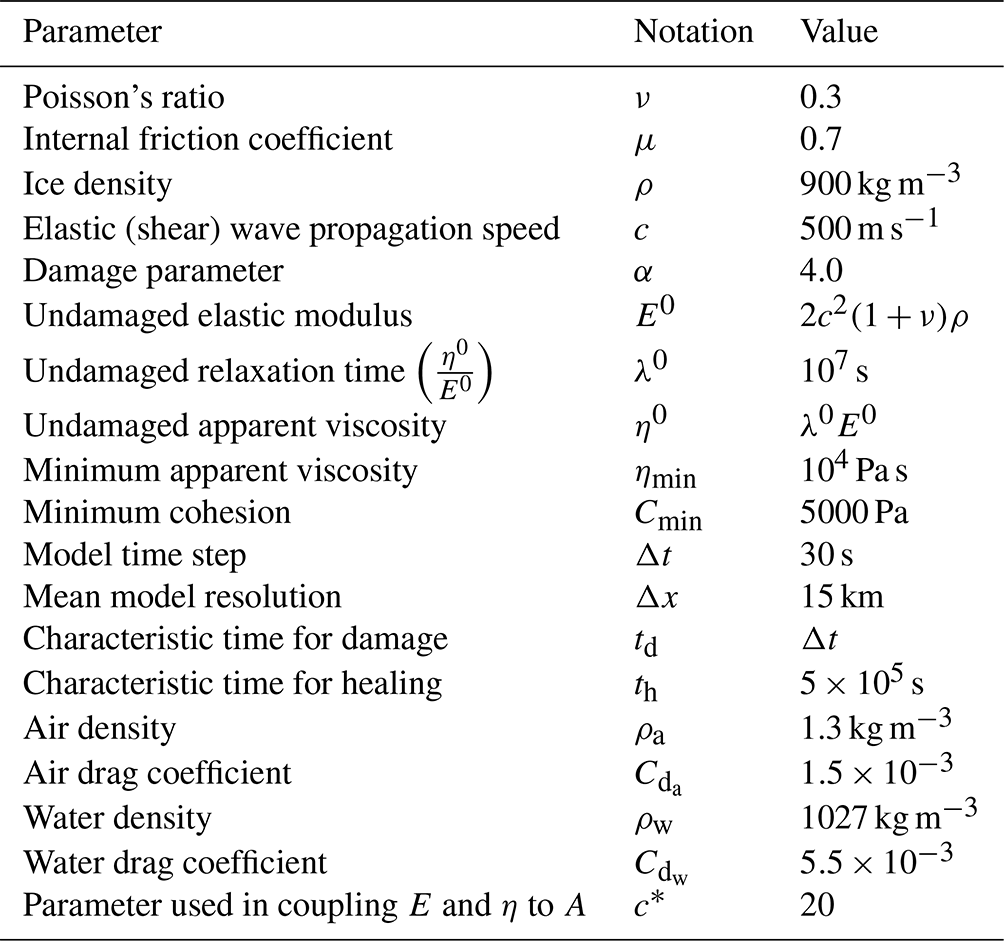
The wind field is prescribed as a series of passing cyclonic storms combined with a constant background wind. To have control over the vorticity and divergence of the wind field, we use the Helmholtz decomposition:

$$\begin{array}{}\text{(B1)}& {\mathbf{u}}_{\mathrm{a}}=\mathrm{\nabla }\mathbf{\Phi }+\mathbf{k}\times \mathrm{\nabla }\mathbf{\Psi },\end{array}$$

where ${\mathbf{u}}_{\mathrm{a}}=(u_{\mathrm{a}},v_{\mathrm{a}})$, Φ is the velocity potential, and Ψ is the streamfunction with the solenoidal wind component ${\mathbf{u}}_{\mathrm{a}}^s=\mathrm{\nabla }\mathbf{\Phi }$ and the divergent wind component ${\mathbf{u}}_{\mathrm{a}}^{\mathrm{d}}=\mathbf{k}\times \mathrm{\nabla }\mathbf{\Psi }$. The equations for the wind field are

$$\begin{array}{}\text{(B2)}& {\displaystyle }{u}_{\mathrm{a}}^{\mathrm{s}}(\widehat{x},\widehat{y},t)=U_{\mathrm{s}}{\sin }^{\mathrm{2}}\left(\mathrm{2}\mathit{\pi }\widehat{x}\right)\sin \left(\mathrm{4}\mathit{\pi }\widehat{y}\right)\cdot \mathit{\gamma }\left(t\right)\cdot U_{\mathrm{mask}},\text{(B3)}& {\displaystyle }{v}_{\mathrm{a}}^{\mathrm{s}}(\widehat{x},\widehat{y},t)=-U_{\mathrm{s}}{\sin }^{\mathrm{2}}\left(\mathrm{2}\mathit{\pi }\widehat{y}\right)\sin \left(\mathrm{4}\mathit{\pi }\widehat{x}\right)\cdot \mathit{\gamma }\left(t\right)\cdot U_{\mathrm{mask}}+U^{\mathrm{b}},\text{(B4)}& {\displaystyle }{u}_{\mathrm{a}}^{\mathrm{d}}(\widehat{x},\widehat{y},t)=U_{\mathrm{d}}{\sin }^{\mathrm{2}}\left(\mathrm{2}\mathit{\pi }\widehat{y}\right)\sin \left(\mathrm{4}\mathit{\pi }\widehat{x}\right)\cdot \mathit{\gamma }\left(t\right)\cdot U_{\mathrm{mask}},\text{(B5)}& {\displaystyle }{v}_{\mathrm{a}}^{\mathrm{d}}(\widehat{x},\widehat{y},t)=U_{\mathrm{d}}{\sin }^{\mathrm{2}}\left(\mathrm{2}\mathit{\pi }\widehat{x}\right)\sin \left(\mathrm{4}\mathit{\pi }\widehat{y}\right)\cdot \mathit{\gamma }\left(t\right)\cdot U_{\mathrm{mask}},\end{array}$$

with $U_{\mathrm{d}}=\mathrm{0.1}\mathrm{m}{\mathrm{s}}^{-\mathrm{1}}$ as the magnitude of the divergent wind, $U_{\mathrm{s}}=\mathrm{22}\mathrm{m}{\mathrm{s}}^{-\mathrm{1}}$ as the maximum solenoidal wind speed and $U^{\mathrm{b}}=\mathrm{2}\mathrm{m}{\mathrm{s}}^{-\mathrm{1}}$ as the background wind field. To simulate a sequence of storms generating and dissipating, we introduce the time-dependent term, γ(t), that controls the strength of the storm:

$$\begin{array}{}\text{(B6)}& \mathit{\gamma }\left(t\right)=\mathrm{1}-\exp \left(-a{\left|\sin \left(\mathit{\pi }{\displaystyle \frac{t}{T}}\right)\right|}^b\right),\end{array}$$

where T is the period of the storm and a=10 and b=2 are parameters that control the shape of the curve and in turn the rate at which the storm is generated, maintains its maximum strength and then dissipates. In Eqs. (B2)–(B5), the spatial coordinate, $({\widehat{x}}_t,{\widehat{y}}_t)$, is time-dependent. This simulates the passing of the storm across the domain.

$$\begin{array}{}\text{(B7)}& {\displaystyle }{\widehat{x}}_t={\widehat{x}}_{t-\mathrm{1}}+\mathrm{\Delta }{\widehat{x}}_t,\text{(B8)}& {\displaystyle }{\widehat{y}}_t={\widehat{y}}_{t-\mathrm{1}}-v_{\mathrm{c}}\mathrm{\Delta }t/L,\end{array}$$

where Δt is the forcing frequency, v_c is the speed at which the storm passes across the domain (from the bottom to top), $L=L_{\max }-L_{\min }$ and $\mathrm{\Delta }{\widehat{x}}_t$ is a random perturbation that allows us to send the storm on a random walk. The initial position of each storm is given by

$$\begin{array}{}\text{(B9)}& {\displaystyle }{\widehat{x}}_{\mathrm{0}}={\displaystyle \frac{(x-x_{\mathrm{c}})-L_{\min }}{L}}-{\displaystyle \frac{\mathrm{1}}{\mathrm{4}}},\text{(B10)}& {\displaystyle }{\widehat{y}}_{\mathrm{0}}={\displaystyle \frac{(y-y_{\mathrm{c}})-L_{\min }}{L}}-{\displaystyle \frac{\mathrm{1}}{\mathrm{4}}},\end{array}$$

where (x_c, y_c) is the initial position of the storm centre. The choice of T; v_c; and x_c,y_c is given in Table 2, and the $\mathrm{\Delta }{\widehat{x}}_t$ related to the random walk is specified in Eq. (4).

With these setups, each storm is approximately half the width of the domain. The sine and cosine equations can generate four storms in the domain, and U_mask is used to ensure only one storm is in the domain at any time:

$$\begin{array}{}\text{(B11)}& U_{\mathrm{mask}}=(\mathrm{1}-\lfloor x\rfloor -\mathrm{2}\left[{\displaystyle \frac{\lfloor x\rfloor }{\mathrm{2}}}\right])H\left(\sin \right(\mathrm{2}\mathit{\pi }x\left)H\right(\sin \left(\mathrm{2}\mathit{\pi }y\right),\end{array}$$

where [] is the integral part function and H(x) is a Heaviside step function.