Simulating lake ice phenology using a coupled atmosphere–lake model at Nam Co, a typical deep alpine lake on the Tibetan Plateau

Simulating the ice phenology of deep alpine lakes is important and challenging in coupled atmosphere–lake models. In this study, the Weather Research and Forecasting (WRF) model, coupled with two lake models, the freshwater lake (WRF–FLake) model and the default lake (WRF–CLake) model, was applied to Nam Co, a typical deep alpine lake located in the centre of the Tibetan Plateau, to simulate its lake ice phenology. Due to the large errors in simulating lake ice phenology, related key parameters and parameterizations were improved in the coupled model based on observations and physics-based schemes. By improving the momentum, hydraulic, and thermal roughness length parameterizations, both the WRF–FLake model and the WRF–CLake model reasonably simulated the lake freeze-up date. By improving the key parameters associated with shortwave radiation transfer processes when lake ice exists, both models generally simulated the lake break-up date well. Compared with WRF–CLake without improvements, the coupled model with both revised lake models significantly improved the simulation of lake ice phenology. However, there were still considerable errors in simulating the spatial patterns of freeze-up and break-up dates, implying that significant challenges in simulating the lake ice phenology still exist in representing some important model physics, including lake physics such as grid-scale water circulation and atmospheric processes such as snowfall and surface snow dynamics. Therefore, this work can provide valuable new implications for advancing lake ice phenology simulations in coupled models, and the improved model also has practical application prospects in weather and climate forecasts.

1 Introduction

Alpine lakes are one key land cover type on the Tibetan Plateau (TP). These lakes serve as a main water supply of the TP, i.e. the “Asia water tower” (Xu et al., 2008), with a total coverage of more than 47 000 km² (Zhang et al., 2019, 2014), which is about 2 % the total area of the TP. Therefore, alpine lakes play a crucial role in local and regional climate through thermal and hydrological cycles in the Earth system. For example, lakes, especially large lakes, can generally enhance and/or change the temporal and spatial distributions of the precipitation over lakes and surroundings through dynamic and thermal processes (Dai et al., 2018b; Su et al., 2020; Wu et al., 2019; Yang et al., 2022; Yao et al., 2021; Zhao et al., 2022). An accurate simulation of lake climatic impacts can enhance the reliability of forecasting results in climate models. However, there are still large uncertainties in the parameterizations of the associated physical processes.

Lakes over middle to high latitudes undergo seasonal freeze–thaw cycles. Due to the large contrast in heat capacity associated with the large water storage per unit area, deep lakes often show significantly different ice phenology characteristics compared to shallow lakes and surrounding land areas. Many alpine lakes are deep lakes with average depths greater than 20 m, such as Qinghai Lake, Nam Co, and Selin Co (Guo et al., 2016; Li et al., 2016; Wang et al., 2009). The ice phenology of alpine lakes can influence not only the lake water and energy budget, but also the seasonality of local and regional climates. For example, lake freeze-up in cold seasons can maintain water levels by preventing evaporation losses in lakes (Lei et al., 2018). The surface evaporation of lakes will significantly increase during the cold ice-free period due to the strong turbulent mixing of lake water, which can provide appropriate moisture conditions for snowfall events.

The freeze-up date of a lake depends on the balance of energy storage. Turbulent heat fluxes play an important role in simulating the energy stored by lake water and thus influence the freeze-up date (Ma et al., 2022; Zhou et al., 2023). The parameterizations of lake surface turbulent heat fluxes may have large uncertainties (Wen et al., 2016), while the formulations of radiation processes at the water surface are relatively stable. Thus, the physical schemes of the heat fluxes need to be accurately parameterized in numerical models. One key parameter in simulating the turbulent heat fluxes is the roughness length, the parameterization of which plays an important role in accurately simulating the turbulent heat fluxes across the North American Great Lakes (Deacu et al., 2012; Charusombat et al., 2018). It was also proven to have significant influence on simulating the freeze-up date of Nam Co (Ma et al., 2022). The melting of lake ice mainly depends on solar-radiation-related processes (Efremova and Pal'shin, 2011; Huang et al., 2022), especially the shortwave processes for ice and water, which are closely related to the albedo and the extinction coefficient (Kirillin et al., 2012; Li et al., 2021). The absorption of the shortwave at the ice surface, deep ice, and water underneath can result in different ice thicknesses and freeze-up dates (Zhou et al., 2023).

Offline lake models show considerable ability to simulate the seasonal freeze-up and break-up dates of alpine lakes (Dai et al., 2018a; A. Huang et al., 2019; W. Huang et al., 2019; Li et al., 2021). However, regional climate and weather forecasts, as well as the lake effect, can be achieved only through a coupled model. Therefore, the application and ability of coupled atmosphere–lake models for deep alpine lakes still needs to be further investigated, as highlighted in previous studies (Su et al., 2020; Wu et al., 2019; Zhou et al., 2023). It is more challenging for a coupled atmosphere–lake model to simulate the ice phenology of alpine lakes, because for offline simulation, the atmospheric forcing is prescribed from observation or reanalysis data, which is a strong constraint on model performance and usually has fatal disadvantages. For example, the shortwave radiation above lake surface can be 100 W m⁻² stronger than that of the surrounding land due to the cloud hole effect (Yao et al., 2023). Thus, simulating lake ice phenology using a coupled model is necessary and important. Furthermore, a coupled model is more sensitive to key parameters and parameterizations, since the long-term integration will increase the model errors through the two-way exchange of energy and water between the atmosphere and the lake surface (Zhou et al., 2023).

Therefore, in this work, the Weather Research and Forecasting (WRF) model coupled with two lake models, the freshwater lake (FLake) model (Mironov, 2008) and the simplified Community Land Model (CLM) lake model (Gu et al., 2015), was applied to a typical deep alpine lake, Nam Co. In Zhou et al. (2023), by multiplying the fraction velocity by a constant, the WRF model can better simulate the surface turbulent heat fluxes and ice phenology of Nam Co. However, such a method is too empirical. The current work is an extension of that work and focuses on revising key parameters and improving key parameterizations using observations and physics-based schemes to better simulate key lake-energy-related processes, for example, turbulent heat fluxes with ice-free conditions and solar radiation transfer with ice-on conditions. The main objectives are to improve the simulation of the lake ice phenology in the WRF model for deep alpine lakes and to suggest important topics for further study into more accurately simulating the lake ice phenology characteristics in coupled atmosphere–lake models. This work is expected to provide an updated model version that can better model the lake-related processes.

2 Study region and data

2.1 Study region

The target lake is Nam Co (Fig. 1a), which is a typical deep lake located in the central TP at approximately 30.7° N, 90.6° E. It covers an area of more than 2000 km² and has an average depth of approximately 40 m (La et al., 2016). This value is calculated from the total water storage (Zhang et al., 2011) divided by lake area. The deepest area is located at the centre of the lake, with a maximum depth of about 100 m. A detailed map of lake bathymetry can be found in previous studies (A. Huang et al., 2019; Wu et al., 2023). Under global warming, the lake water level has experienced a rapid increase since the 1990s due to the increase in precipitation and the increasing water supplied by melting snow and glaciers within the basin (Lei et al., 2014, 2013; Zhang et al., 2020).

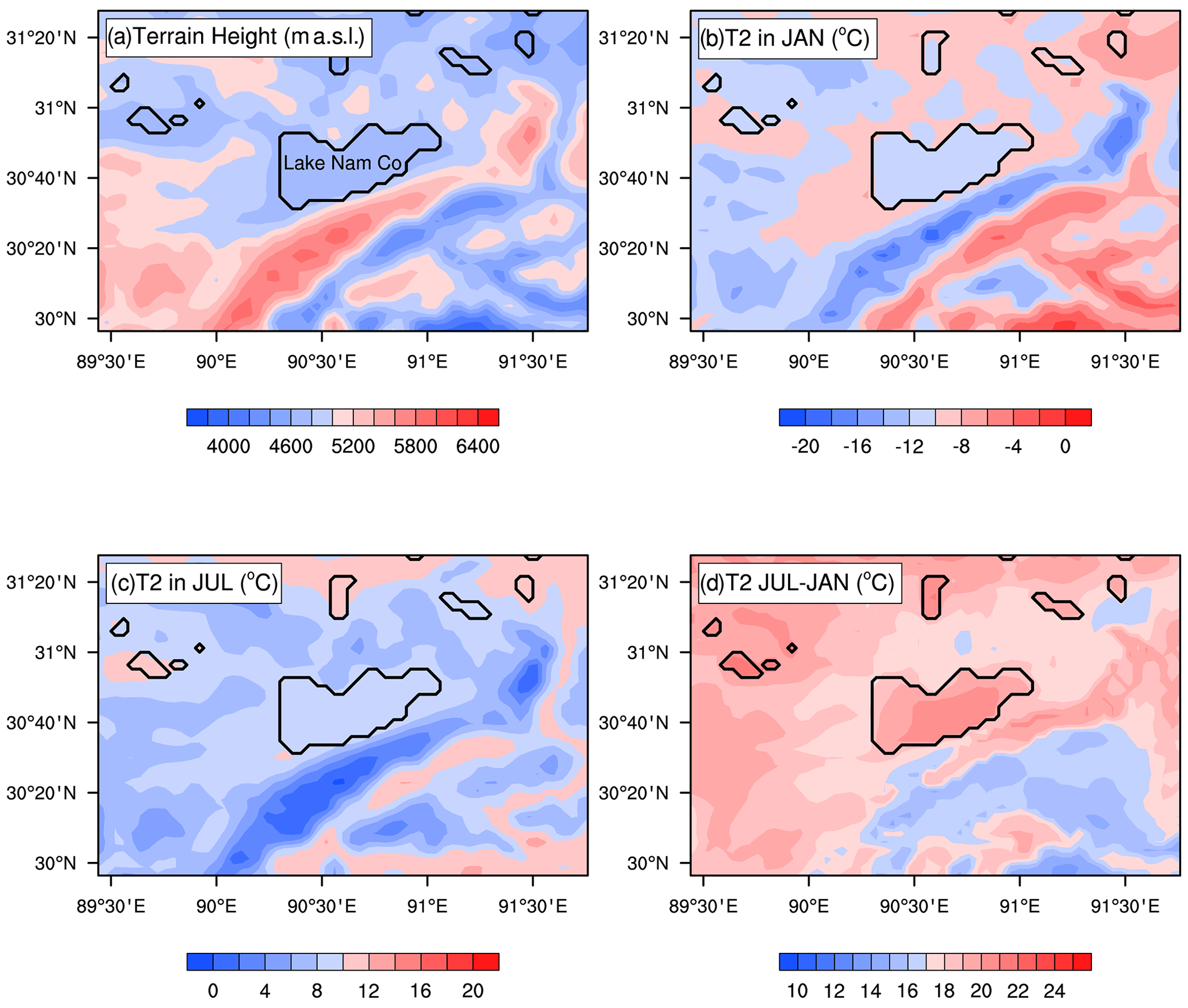
Figure 1 (a) The study region and the simulation domain of the current study, with Nam Co located in the centre – black contour lines denote the lake mask and colour shading denotes the terrain elevation (metres above sea level); the monthly averages of 2 m air temperature (T2 in °C) in (b) January and (c) July (colour shading) derived from default WRF simulation; and (d) the difference in T2 (°C) between July and January (colour shading).

Seasonally, the study region undergoes large temperature variation with a cold monthly mean air temperature generally below 0 °C in January (Fig. 1b) and a warm monthly mean air temperature generally above 0 °C in July (Fig. 1c). Large air temperature difference between the 2 months can reach more than 22 °C (Fig. 1d), indicating a strong seasonality, and thus the physical processes related to the ice–water phase change may play an important role in the water and energy cycles within the study region. For example, compared with open water, a frozen lake has much weaker evaporation and energy release to the atmosphere, and thus the climate effect of lakes will weaken simultaneously. Lakes over this region undergo typical freezing and melting cycles.

2.2 Data

The lake water temperature (TW) data observed in Nam Co cover a period from November 2011 to June 2014 (Wang, 2020). These data are the daily average water temperature data at different depths (3, 6, 16, 21, 26, 31, 36, 56, 66, and 83 m) and were obtained through field monitoring. The data were continuously recorded by deploying water quality multi-parameter probes (CTD 90M, Germany) and temperature thermistors (VEMCO Minilog-II-T, Canada; accuracy: ±0.1 °C from −5 to 35 °C; resolution: 0.01 °C) in the water. The daily average water temperature was calculated based on the original observed data. In the current work, the TW was used for model evaluation. Only the data from the period of 1 July 2013 to 30 June 2014 were used, because the station data after 1 July 2014 are not available due to the instrument damage.

The MODIS lake surface temperature (LST) product was used for comparison with the model results. The 0.05° Aqua and Terra daily datasets were used in the current study (Wan et al., 2015). For a fair comparison, the MODIS data were interpolated to the model grid by the area-weighted method. Due to the contamination by clouds, MODIS has missing observations at a considerable number of pixels. Thus, the mean LSTs were calculated and compared with those from each simulation. For quality control, the LSTs with a fraction of missing observations larger than 90 % were removed. Nonetheless, there were still some outliers especially for nighttime data. Additionally, the land–water mixed pixels (the nearest 2 pixels to land) in MODIS were excluded and a total of 1574 grid points were used.

ERA-Interim reanalysis data (Dee et al., 2011) from the European Centre for Medium-Range Weather Forecasts (ECMWF) were used for the model's initial and lateral boundary forcing conditions. The model was developed based on the Integrated Forecasting System (IFS) model assimilating multisource observations. These data have a resolution of approximately 80 km (T255 spectral) on 60 vertical levels from the surface up to 0.1 hPa.

3 Model description and setup

3.1 WRF model and model setup

In this study, two lake models were used in the coupled atmosphere–lake model to demonstrate the universality of the revisions in parameterization schemes for improving the simulation of lake ice phenology characteristics. One is the FLake model and the other one is the simplified CLM lake model. These two models are coupled with WRF and referred to as WRF–FLake and WRF–CLake hereafter. The default WRF was developed by NCAR. It is a nonhydrostatic model with multiple schemes in the planetary boundary layer, the land surface model, the cloud microphysics, the cumulus convection, and the orographic drag. In this study, WRF3.9 (Skamarock et al., 2008) was applied to the TP region.

The two lake models have been coupled with WRF in a one-dimensional way; i.e. no horizontal water flow is simulated. In the coupling strategy, a grid point with 50 % lake cover is defined as a lake point. At each time step, lake models are driven by atmospheric forcing including air temperature, pressure, humidity, wind, shortwave and longwave radiation, precipitation, and reference height (height of first atmospheric layer). Simultaneously, the lake models feed back momentum, sensible heat, and latent heat fluxes to the atmosphere part of WRF model.

Figure 1a shows the simulation domain, covering Nam Co and the surrounding land. The WRF model setup is generally consistent with Zhou et al. (2023), with a horizontal grid spacing of 0.04° (approximately 4.5 km), which is identified as convection-permitting. The coupled modes were run with a time step of 10 s. There are 116 lake grid points in the model. The lateral boundary conditions were provided at 6-hourly intervals. The simulations were performed for 2 years from 1 July 2013 to 30 June 2015. The lake water temperature in the coupled model was initialized at 00:00 UTC on 1 July 2013 using MODIS observations. The water temperature at the first layer is set to MODIS-observed values, while the water temperature at the other layers is linearly interpolated with depth under the assumption that the water temperature at the deepest layer is equal to 3.5°C (the temperature at maximum water density). The other variables in the coupled model are initialized by ERA-Interim data at the same time. Based on previous studies over the TP, a turbulent orographic form drag scheme was used to represent the subgrid orographic drag (Zhou et al., 2017, 2021), the Dudhia scheme (Dudhia, 1989) and the RRTM (Mlawer et al., 1997) were used for shortwave and longwave radiation transfer, the modified Thompson scheme (Thompson et al., 2008) was used for the microphysics, Noah-MP (Niu et al., 2011; Yang, 2011) was used for the land surface processes, and the Mellor–Yamada–Janjić turbulent kinetic energy scheme (Janjić, 2001; Mellor and Yamada, 1974) was used for the planetary boundary layer.

Three experiments were designed in the current study. One used the WRF coupled with the default lake model without revisions of key lake parameters and parameterizations, which was defined as the control run (WRF–Ctrl). The other two used WRF coupled with the revised FLake model and revised default lake model, defined as the WRF–FLake run and the WRF–CLake run. The unrevised version of the WRF–FLake model was not selected as a control run because it had difficulties simulating the ice phenology characteristics; i.e. a considerable number of lake grid points never freeze up and/or never break up after freeze-up (Zhou et al., 2023).

3.2 Lake models and model setup

FLake is a freshwater model developed by Mironov (2008). It is not designed with explicit fixed depth layers. There is an upper mixed layer and a thermocline layer in which the water temperature is parameterized by the self-similarity theory. One key feature of FLake is that the mixed layer depth is parameterized by diagnosing the water stability conditions, which is different from the finite-difference model in which the energy exchange is parameterized by a turbulent mixing ratio. FLake was coupled with WRF by Zhou et al. (2023) to perform sensitivity studies of key physical processes in simulating lake ice phenology. This study used the same version.

The other lake model is the default one in WRF, which is a simplified version of the CLM lake model. It is a finite-difference model that was originally designed for shallow lakes. It has 10 vertical layers, and the water turbulent mixing ratio is empirically set to a constant between the layers. The CLM lake model is simplified and coupled with WRF by Gu et al. (2015) to describe lake processes in the WRF model.

Previous studies have shown that using the default settings in lake models can lead to considerable errors in the simulations (A. Huang et al., 2019; Ma et al., 2022; Zhou et al., 2023). Thus, some key parameters and physical schemes were revised based on previous studies. For both lake model setups in the coupled model, the lake depth was set to the average value of 40 m for all lake grid points, which was consistent with the offline lake model simulations by La et al. (2016). Thus, to save computational expense, their simulation results were used to initialize the lake water temperature in the coupled model. Noting that both lake models used in the current study are one-dimensional models, no horizontal water flow is simulated in the coupled model. Such a model setup is a general way for modelling lake processes in a climate model, such as the Community Earth System Model (CESM), Consortium for Small-scale Modelling (COSMO), and WRF model. The setup of the following parameters is based on observation. The water extinction was set to 0.12 according to Wang et al. (2009) and A. Huang et al. (2019). The temperature at maximum water density was set to 3.5°C according to J. B. Wang et al. (2019) and Wu et al. (2019).

3.3 Model improvements and limitations

In the default WRF–CLake model, the momentum, hydraulic, and thermal roughness lengths were set to constant values of 0.001. In the default FLake model, the roughness length for momentum (z_0m) is parameterized as follows:

$$\begin{array}{}\text{(1)}& z_{\mathrm{0}\mathrm{m}}=\mathit{\alpha }\times {\displaystyle \frac{u_{\ast }^{\mathrm{2}}}{g}},\end{array}$$

where α is the Charnock number calculated by $\mathit{\alpha }=\mathrm{0.0012}+\mathrm{0.7}\times (\mathrm{1}/\mathrm{1000}\times (u^{\mathrm{2}})/g)$, u is the surface wind speed, u_∗ is the surface friction velocity in m s⁻¹, and g=9.8 m s⁻² is the gravitational acceleration constant. Then, the hydraulic roughness length z_0q is further parameterized as follows:

$$\begin{array}{}\text{(2)}& z_{\mathrm{0}q}=z_{\mathrm{0}\mathrm{m}}\times \exp \left(-C_{\mathrm{k}}\times \left(\mathrm{4.0}\times {\left({\displaystyle \frac{u_{\ast }^{\mathrm{3}}}{g\times \mathit{\nu }}}\right)}^{\mathrm{0.5}}-\mathrm{4.2}\right)\right),\end{array}$$

where C_k=0.4 is the von Kármán constant, ν is the kinematic viscosity of air, and the thermal roughness length z_0h is further parameterized as

$$\begin{array}{}\text{(3)}& z_{\mathrm{0}h}=z_{\mathrm{0}\mathrm{m}}\times \exp \left(-C_{\mathrm{k}}\times \left(\mathrm{4.0}\times {\left({\displaystyle \frac{u_{\ast }^{\mathrm{3}}}{g\times \mathit{\nu }}}\right)}^{\mathrm{0.5}}-\mathrm{3.2}\right)\right).\end{array}$$

The above formulation is used in Zhou et al. (2023), which introduced large model errors in simulating lake ice freeze-up time. The reason is that such a parameterization simulated turbulent heat fluxes that were too weak, which controls the lake water energy balance. Empirically, these fluxes have also increased 1.5 times to improve the model performance. Nevertheless, such an empirical method lacks a physical basis and is model dependent. In the current study, differently from such methods, an observation-based roughness length scheme for open water (B. B. Wang et al., 2019) was used for both WRF–CLake and WRF–FLake, which have been proven to be able to better simulate the heat fluxes and lake freeze-up date in WRF–CLake (Ma et al., 2022). z_0m is parameterized as follows:

$$\begin{array}{}\text{(4)}& z_{\mathrm{0}\mathrm{m}}=\mathit{\alpha }\times {\displaystyle \frac{u_{\ast }^{\mathrm{2}}}{g}}+R_r\times {\displaystyle \frac{\mathit{\nu }}{u_{\ast }}},\end{array}$$

where α=0.031 and R_r=0.54. These two parameters are calibrated using field observations at Nam Co (B. B. Wang et al., 2019). ν is the kinematic viscosity of air, u_∗ is the surface friction velocity in m s⁻¹, g=9.8 m s⁻¹² is the gravitational acceleration constant, and $R_e=u_{\ast }{z}_{\mathrm{0}\mathrm{m}}/\mathit{\nu }$ is the roughness Reynolds number. Then, the hydraulic and thermal roughness lengths z_0q and z_0h are further parameterized as follows:

$$\begin{array}{}\text{(5)}& z_{\mathrm{0}q}=z_{\mathrm{0}h}=z_{\mathrm{0}\mathrm{m}}\times \exp \left(-\mathrm{2.67}\times R_e^{\mathrm{0.25}}+\mathrm{0.57}\right),\end{array}$$

where $R_e=u_{\ast }{z}_{\mathrm{0}\mathrm{m}}/\mathit{\nu }$ is the Reynolds number.

In the default WRF–CLake model, the division of the vertical layers of the lake is four layers (Ma et al., 2022). In the current work, to better simulate the lake ice break-up date, the division of the vertical layers of the lake in WRF–CLake was revised to 10 layers according to CLM4.5. During freeze-up, if the ice is covered with snow, then the lake surface albedo is set to the snow albedo. The default ice albedo in WRF–CLake is 0.6. In the current study, it was set to 0.55 with the consideration that 0.5–0.6 is the most distributed range of albedo observations for Nam Co, as investigated in Li et al. (2018). In WRF–FLake, the albedo α is parameterized by the ice surface temperature as follows:

$$\begin{array}{}\text{(6)}& \mathit{\alpha }={\mathit{\alpha }}_{\max }-({\mathit{\alpha }}_{\max }-{\mathit{\alpha }}_{\min })\exp (-\mathrm{95.6}(T_{\mathrm{f}}-T_{\mathrm{s}})/T_{\mathrm{f}}),\end{array}$$

where α_max and α_min are the maximum and minimum ice albedo, respectively; T_f=273.15 is the temperature at the freezing point; and T_s is the ice surface temperature. In Zhou et al. (2023), the default values of α_max and α_min were set to 0.2 and 0.1, respectively, with the consideration of ice albedo variance under snow-free conditions. Nevertheless, the value of 0.2 is too small under all conditions (when snow often appears), as seen in satellite observations (Li et al., 2018). Therefore, in the current study, α_max is revised to 0.75 based on satellite observations (Li et al., 2018). In their study, the occurrence of maximum albedo during the ice-on season at Nam Co is no more than 0.8 based on MODIS data. Such treatment of lake surface albedo directly takes into account the influence of snow on lake surface albedo. Therefore, we can make sure that the modelled snowfall biases will not directly introduce uncertainties in simulating the lake processes. Over the complex terrain region, precipitation is a great challenge, and it is very difficult to correctly simulate precipitation amount. In TP, there is a systematic overestimation of precipitation in climate models (Gao et al., 2015; Su et al., 2013). Additionally, considering that the absorption of shortwave radiation at the ice surface is also an important parameter, it is revised to 0.65 according to a sensitivity study similar to that in Zhou et al. (2023). In the sensitivity study, all the simulations are initialized on 1 January 2014, a few days before lake freeze-up, which ensures the lake water thermal status and the freeze-up dates are correct at the initial stage. Before freeze-up, the lake water is fully mixed and a uniform temperature initialization is reasonable. With an ice surface absorption ratio of 0.65, the model shows the best performance in simulating the lake ice break-up date compared with other values (0.5, 0.55, 0.6, 0.7, and 0.75).

3.4 Calculation of the lake freeze-up date and break-up date

The freeze-up date at each grid point is defined as the first day when lake ice occurs with no ice-free days in the following 20 d at this grid point, while the break-up date at each grid point is defined as the first day when ice-free occurs after 20 ice-on days at this grid point. The freeze-up duration at each grid point is defined as the number of days with continuous ice cover at this grid point. It is derived from the break-up date minus the freeze-up data. At each model grid point, there are 16 (4 × 4) co-located MODIS pixels. Thus, for the calculation of freeze-up date and break-up date by MODIS, the maximum LST at each grid point is selected from the 16 co-located MODIS pixels. The reason for using maximum LST rather than an average is that MODIS data may be contaminated by cloud top temperature, which could be much colder than real lake surface temperature. Additionally, such a treatment can preserve satellite information to maintain maximally continuous time series within the grid points. Even though there are freeze-up dates and break-up dates, in a considerable number of model grid points, they cannot be effectively calculated due to too many missing observations in MODIS. The number of lake grid points with missing values is even larger when calculating the freeze-up durations by subtracting the break-up date and freeze-up date.

Treating the lake as a whole, the lake freeze-up date and lake break-up date are calculated based on the lake frozen fraction. The lake frozen fraction is defined as the ratio of the number of ice-on grid points to all grid points. The lake freeze-up date is defined as the first day when the lake frozen fraction reaches 90 % and does not fall below this threshold for 20 consecutive days, while the lake break-up date is defined as the first day when the lake frozen fraction falls below 90 % and never exceeds this threshold for 20 consecutive days. Lake freeze-up duration is derived from the lake break-up date minus the lake freeze-up date.

4 Results and analysis

4.1 Surface heat flux and water temperature

Previous studies show that there are large uncertainties in simulating turbulent heat fluxes in lake models (Wen et al., 2016). Additionally, turbulent heat fluxes play key roles in simulating the lake water temperature and lake freeze-up date (Ma et al., 2022; Zhou et al., 2023). In contrast, other energy components at the lake surface are relatively more reasonably simulated due to reliable observations of related parameters. For example, regarding shortwave and longwave radiation, the albedo for open water is approximately 0.08 and the emissivity is approximately 0.98. These two key parameters have low uncertainties and can be accurately estimated. Therefore, only the simulated turbulent heat fluxes and water temperature were investigated in this section.

To demonstrate the effects of model improvements, Fig. 2 shows the differences in daily mean sensible heat and latent heat derived from WRF–FLake and WRF–CLake minus WRF–Ctrl at Nam Co and averaged over all lake grid points. Compared with WRF–Ctrl, both WRF–FLake and WRF–CLake show smaller differences in simulating the sensible heat for ice-free periods (Fig. 2a), while they show considerably larger negative differences in simulating the latent heat for ice-free periods, especially within approximately 1 month before ice-on (Fig. 2b), indicating that the latent heat is more sensitive to the improvements in the hydraulic and thermal roughness length parameterizations as introduced in Sect. 3.2. The improved model WRF–FLake and WRF–CLake show quite good agreement with each other, because both models used the same parameterizations of momentum and thermal roughness lengths (Sect. 3.2). Both WRF–FLake and WRF–CLake obviously show larger sensible heat and latent heat in November–December than WRF–Ctrl due to the early freeze-up in the WRF–Ctrl model. The differences in sensible heat and latent heat at the initial stages of ice-on between the two improved models could be associated with the inconsistency in the freezing status of specific grid points between the two simulations. Additionally, other thermal processes (such as water turbulent mixing) also play certain roles and caused different model performances in simulating sensible heat, latent heat, and lake freeze-up time. Obviously, the smaller latent heat during ice-free periods in WRF–FLake and WRF–CLake simulations leads to a weaker water energy release, resulting in a late freeze-up.

The sensible heat and latent heat control the atmosphere–lake energy exchange and lake water energy storage and thus influence the lake freeze-up date (Ma et al., 2022; Zhou et al., 2023). In the following, the LST and water temperature profiles are compared with MODIS and station observations, respectively.

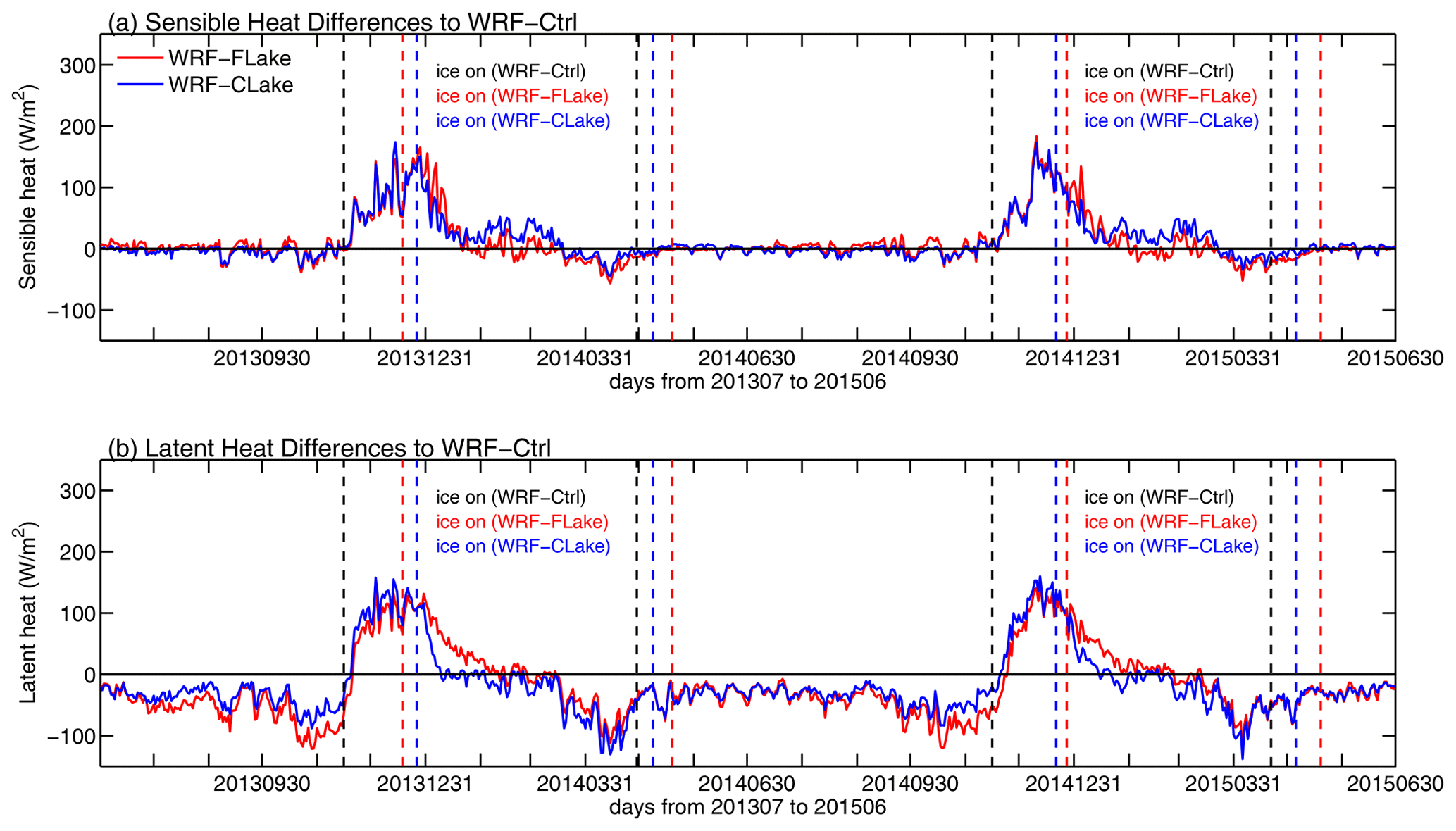
Figure 2 Differences in the daily mean (a) sensible heat and (b) latent heat derived from WRF–FLake and WRF–CLake minus WRF–Ctrl at Nam Co and averaged over all lake grid points for the study period. The vertical lines show the first and last days of ice occurrences in each simulation (black: WRF–Ctrl; red: WRF–FLake; blue: WRF–CLake).

Figure 3a shows the time series of mean LST biases (averaged over the grid points with MODIS observation) in each simulation (WRF–Ctrl, WRF–FLake, and WRF–CLake minus MODIS) for the study period. The biases are derived from WRF–Ctrl, WRF–FLake, and WRF–CLake runs minus MODIS. WRF–Ctrl obviously shows cold biases during ice-free periods. These cold biases (for example, in September and October) are alleviated in the WRF–FLake and the WRF–CLake runs. Considering the uncertainties in the MODIS products – that is, there are obvious unreliable underestimations of nighttime LST for alpine lakes including Nam Co (La et al., 2022) – slight warmer biases in LST are expected during ice-free periods as shown in the WRF–FLake and WRF–CLake runs in Fig. 3a. Larger cold biases in WRF–Ctrl occur in November–December due to the early ice-on, which is significantly improved in the WRF–FLake and the WRF–CLake runs. At the time of early ice-on in these two runs, the simulated LSTs also show cold biases. The reason could be that for MODIS only ice-free pixels were averaged because the freeze-up pixels were hard to distinguish between the lake surface or the cloud top, which also explains the continuous missing observations of MODIS during lake freeze-up. Therefore, the LST during early ice-on stage is logically incomparable between the model simulations and MODIS. Figure 3b shows the differences in the daily mean LST (averaged over all grid points) derived from WRF–FLake and WRF–CLake minus WRF–Ctrl for the study period. The WRF–FLake and WRF–CLake runs obviously have warmer LSTs during ice-free periods, which can be explained by the stronger cooling effect due to the larger latent heat release as shown in Fig. 2b. The largest LST differences in WRF–FLake and WRF–CLake in November–December are caused by the early ice-on in WRF–Ctrl.

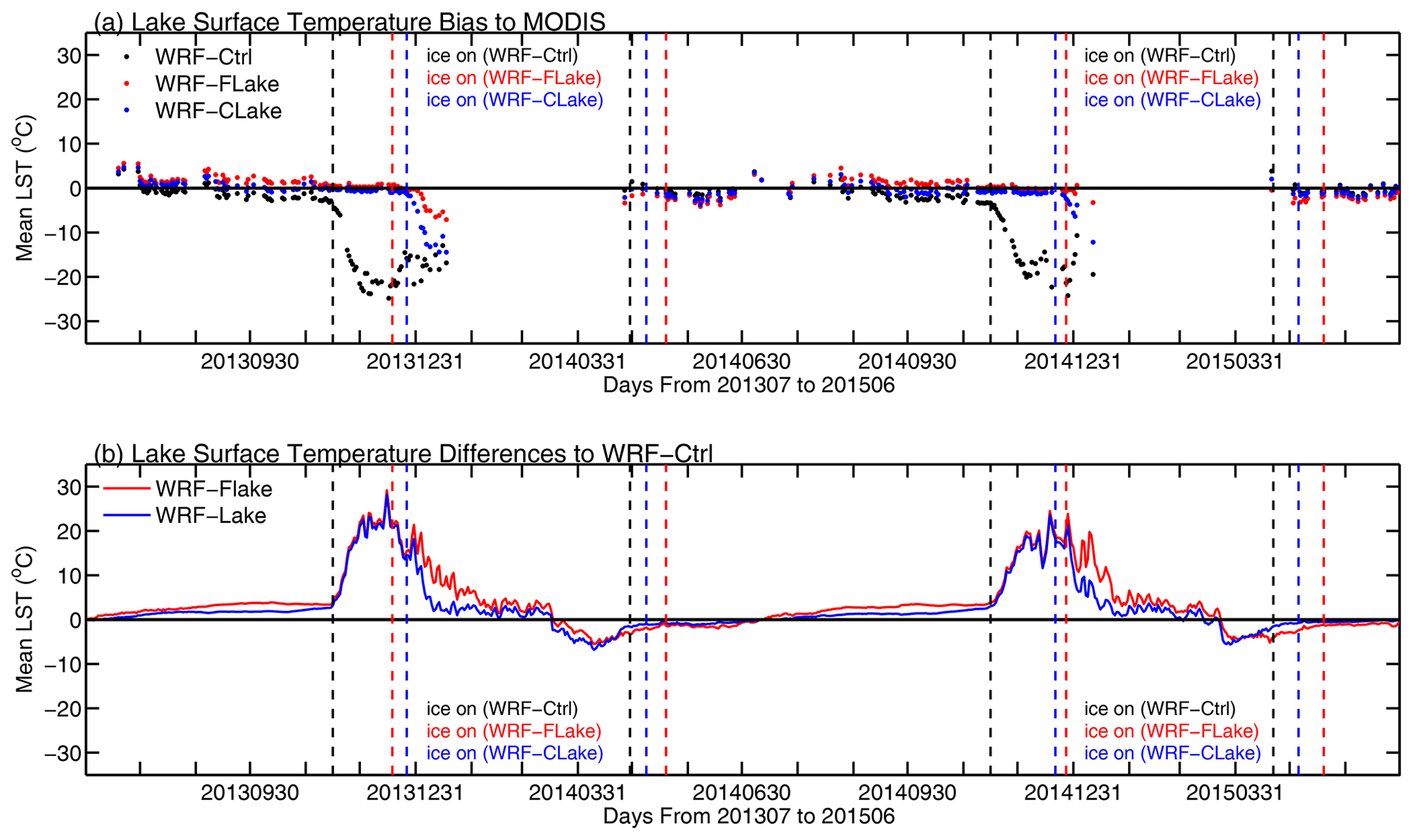
Figure 3 (a) The biases in daily mean LST to MODIS in each simulation (black: WRF–Ctrl; red: WRF–FLake; blue: WRF–CLake) for the study period and (b) the differences in the daily mean LST derived from WRF–FLake and WRF–CLake minus WRF–Ctrl for the study period. The biases are derived from WRF–Ctrl, WRF–FLake, and WRF–CLake runs minus MODIS. The differences are derived from WRF–FLake and WRF–CLake runs minus the WRF–Ctrl run. The vertical lines show the first and last days of ice occurrences in each simulation (black: WRF–Ctrl; red: WRF–FLake; blue: WRF–CLake).

Figure 4 shows the observed and simulated lake water temperature profiles. Only the data from the period of 1 July 2013 to 30 June 2014 were used, because the station data after 1 July 2014 were not available due to instrument damage. All the simulations can generally simulate the seasonality of the water temperature, with the maximum occurring in August–September and the minimum occurring in winter and early spring. Consistent with the investigation in J. B. Wang et al. (2019), obvious water stratification lasts from July to late October, while the body of water is sufficiently mixed after that time until May of the next year (Fig. 4a). During the ice-on period, the thermal structure of the water column is weakly stratified rather than mixed (Lazhu et al., 2021). The stratification characteristics in the simulations generally agree well with the measurements (Fig. 4b–d). Additionally, the mean bias and root mean square error (RMSE) are calculated (Fig. 4e–f). The WRF–Ctrl and WRF–CLake runs show cold biases, especially at shallow layers, while WRF–FLake has smaller mean bias errors (Fig. 4e). By revising key parameters and improving key parameterizations of lake models (as in Sect. 3.2 and 3.3), the cold biases can be effectively alleviated. The RMSE in WRF–FLake is larger at deep layers, indicating a worse performance, with the opposite at shallow layers (Fig. 4f). The mean bias in WRF–FLake is smaller than that in WRF–Ctrl and WRF–CLake, while the RMSE is larger for some layers. This could be associated with the differences in seasonal variation in the LST between the models and observations. That is, WRF–FLake (Fig. 4c) is much warmer in summer and colder in winter than WRF–CLake (Fig. 4d) compared with the observations (Fig. 4a). When calculating the mean bias, the more extreme warm bias and cold bias in WRF–FLake compensate for each other. Generally, the errors in simulating the lake water temperature are at reasonable scales compared with offline lake model simulation results in other studies (La et al., 2016; A. Huang et al., 2019), which show RMSEs within the intervals of 1.0–2.5 and 1.8–2.4 °C.

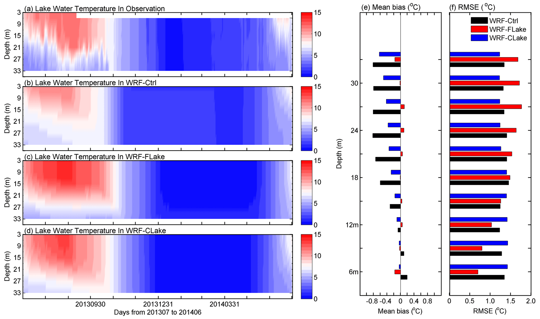
Figure 4 Lake water temperature profiles in (a) station observations and each simulation (b: WRF–Ctrl; c: WRF–FLake; d: WRF–CLake) for the period of 1 July 2013 to 30 June 2014 and (e–f) error metrics (mean bias and RMSE) at different depths.

4.2 Lake ice phenology characteristics

In this section, the simulated lake ice phenology is investigated, including the lake frozen fraction, ice thickness, freeze-up and break-up dates of the lake as a whole and for each lake grid, and freeze-up duration. Following the method in Zhou et al. (2023), the ice phenology of Nam Co as a whole is investigated, including the frozen fraction, the mean ice thickness, and the penetrating shortwave radiation at the ice surface. Figure 5a shows the frozen fraction and mean ice thickness of Nam Co in each simulation. Based on MODIS, Nam Co generally freezes in January and breaks in late April (Fig. 5a). For seasonality of lake ice phenology, the WRF–FLake and the WRF–CLake runs generally show good agreement with MODIS, while WRF–Ctrl shows freeze-up and break-up dates that are too early (Fig. 5a). For ice thickness, WRF–FLake simulates thicker ice than WRF–CLake, with maximum thicknesses of approximately 0.5 and 0.4 m, respectively (Fig. 5b). The reason could be attributed to more penetrating shortwave radiation at the ice surface (Fig. 5c), and this part of the energy is more effective in contributing to ice melting in the model as interpreted by Zhou et al. (2023). Compared with these two runs, WRF–Ctrl has much smaller ice thickness, which maintains a constant thickness during the main freeze-up period. This is because the thickness of the second layer was set to 4.0 m by default, which is too deep and difficult to freeze. Additionally, the lake freeze-up and break-up dates and the freeze-up durations derived from each simulation are compared with those from MODIS, as shown in Table 1. Generally, WRF–Ctrl shows freeze-up and break-up dates more than 1 month earlier than MODIS, while both revised models simulate the lake freeze-up and break-up dates with acceptable accuracy (errors smaller than 11 d), except for the break-up date in winter of 2014–2015 in WRF–CLake (Table 1). WRF–Ctrl shows freeze-up durations that are too long and are effectively reduced in WRF–FLake and WRF–CLake runs, though with freeze-up durations that are too short in WRF–CLake (Table 1). This result indicates that, regarding lake freeze-up and break-up dates, the performances of WRF–FLake and WRF–CLake were significantly improved by revising key parameters and improving key parameterizations in lake models.

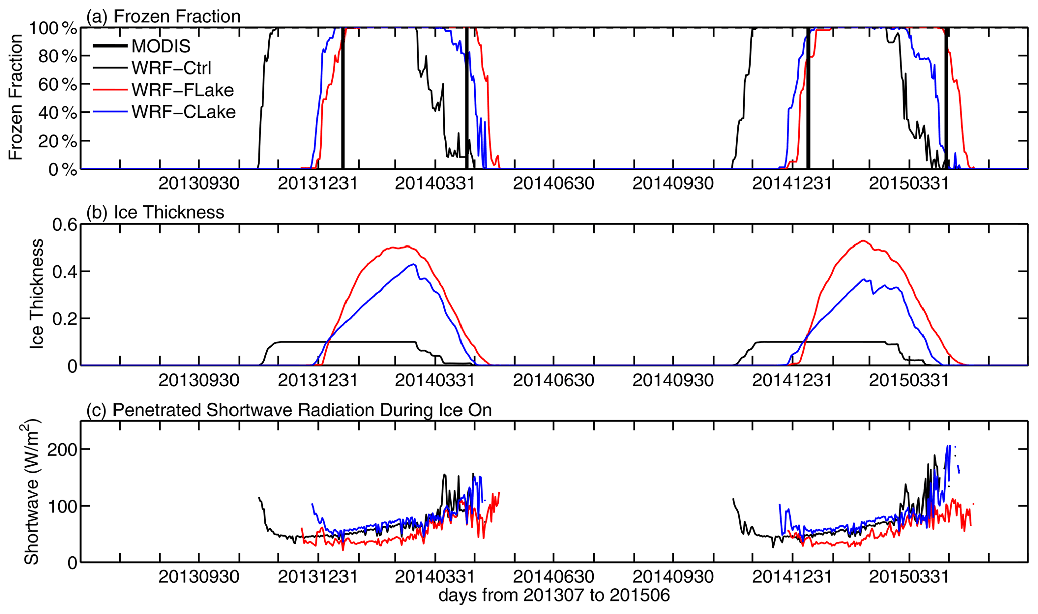
Figure 5 (a) Lake frozen fraction, (b) ice thickness, and (c) penetrating shortwave radiation (during the ice-on period) in each simulation. The vertical bold straight line indicates the freeze-up date and break-up date derived from MODIS.

Table 1 The comparisons of lake freeze-up dates, lake break-up dates, and lake freeze-up durations (days) between each simulation and MODIS; the values indicate the number of days since 1 July of the corresponding year; the values in parentheses indicate the errors of each simulation compared to MODIS; the Julian days of the freeze-up dates and break-up dates are provided for MODIS. Bold indicates a best performance.

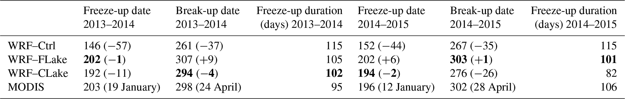
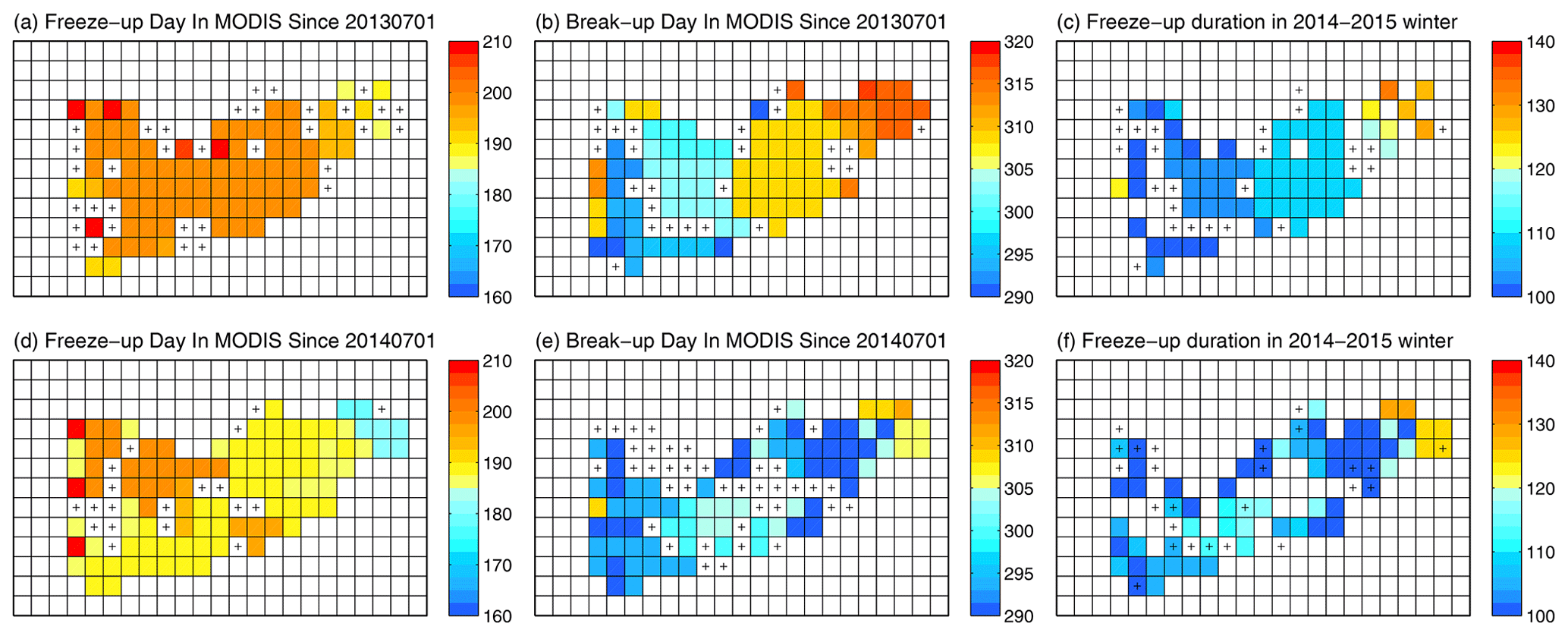
Figure 6 Spatial distribution of the freeze-up date (a, d), break-up date (b, e), and freeze-up duration (c, f) at Nam Co derived from MODIS in the period of (a–c) 2013–2014 and (d–f) 2014–2015. The cross marks denote lake grid points with missing observations in MODIS.

Figure 6 shows the spatial distribution of the freeze-up date, break-up date, and freeze-up duration derived from MODIS data in the winters of 2013–2014 and 2014–2015. There are missing values at considerable grid points due to the missing LST observation by MODIS. Generally, the east of Nam Co shows a little earlier freeze-up time than the west, while the west of Nam Co shows a much earlier break-up time than the east. As a result, the east of Nam Co has longer freeze-up duration. The freeze-up date, break-up date, and freeze-up duration in MODIS are used to quantitatively evaluate the simulations. The inconsistencies in spatial distribution of these three variables between simulations and MODIS are discussed in the next section.

Figure 7 shows the spatial distribution of the freeze-up date in each simulation. WRF–Ctrl predicted early freeze-up, while both revised models are consistent and show late freeze-up in eastern Nam Co and early freeze-up in the middle of the lake for winters of 2013–2014 and 2014–2015. Additionally, WRF–FLake predicted a slightly later freeze-up date than WRF–CLake. Figure 8 shows the spatial distribution of biases in freeze-up date in each simulation derived from WRF–Ctrl, WRF–FLake, and WRF–CLake runs minus MODIS. A positive value indicates a later freeze-up, while a negative value indicates an earlier freeze-up. Compared with MODIS, WRF–Ctrl predicted a freeze-up date that was systematically too early by more than 30 d, while the WRF–FLake and WRF–CLake runs show considerably smaller biases within ±20 d, with negative biases over the mid-western lake and positive biases over the eastern lake except for the freeze-up date in 2014–2015 in the WRF–FLake. Generally, the variability in the biases is low (blue text in Fig. 8), indicating a reliable quantification.

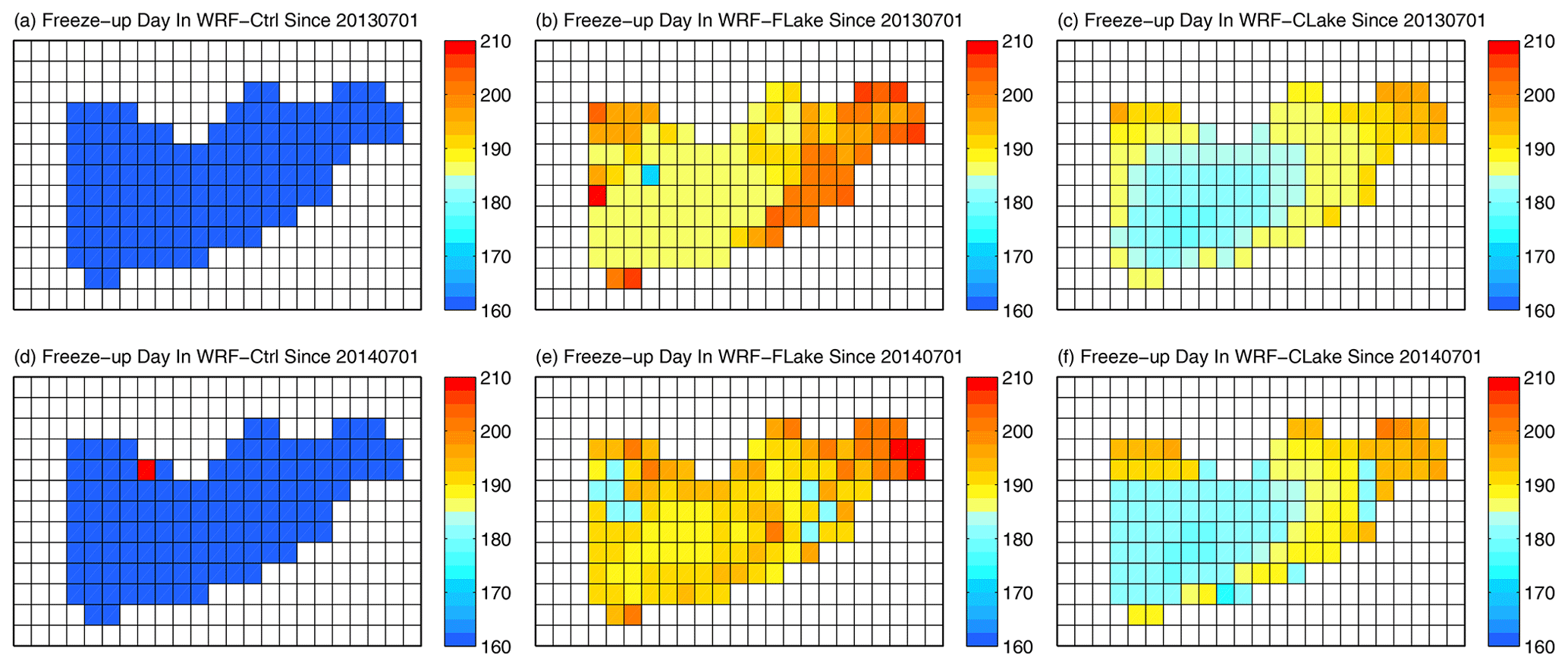
Figure 7 Spatial distribution of the freeze-up date at Nam Co in each simulation in the winters of (a–c) 2013–2014 and (d–f) 2014–2015. The colour indicates the number of days since 1 July in the corresponding year.

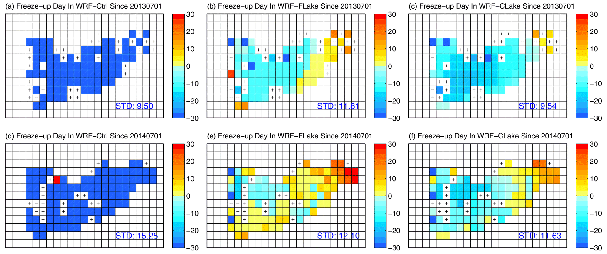
Figure 8 Spatial distribution of biases (days) in freeze-up date at Nam Co in each simulation in the winters of (a–c) 2013–2014 and (d–f) 2014–2015. The biases are derived from WRF–Ctrl, WRF–FLake, and WRF–CLake runs minus MODIS. The cross marks denote lake grid points with missing observations in MODIS.

Figure 9 shows the spatial distribution of the break-up date in each simulation. WRF–Ctrl predicted early break-up, while both revised models show late break-up in western Nam Co and early break-up in the middle for the springs of 2014 and 2015. The break-up being too early in WRF–Ctrl could be associated with the ice being too thin during freezing, and the ice–water phase change requires much less energy and thus a short time. Additionally, WRF–FLake predicted a slightly later break-up date than WRF–CLake, which could be associated with the lake ice thickness in both runs. WRF–FLake has thicker ice during freezing, more energy is required for the ice–water phase change, and thus it takes a longer time. Figure 10 shows the spatial distribution of biases in break-up date in each simulation. Compared with MODIS, WRF–Ctrl predicted a break-up date that was systematically too early by approximately 10–20 d, while the WRF–FLake and WRF–CLake runs show late break-up dates over the mid-western lake (more than 20 d and 0–10 d, respectively) and early break-up dates over the eastern lake (−10 to 0 d and smaller than −20 d, respectively). Generally, the variability in the biases in break-up date (blue text in Fig. 10) is a little higher than the variability in the biases in freeze-up date, which could be due to more missing values in the MODIS break-up date.

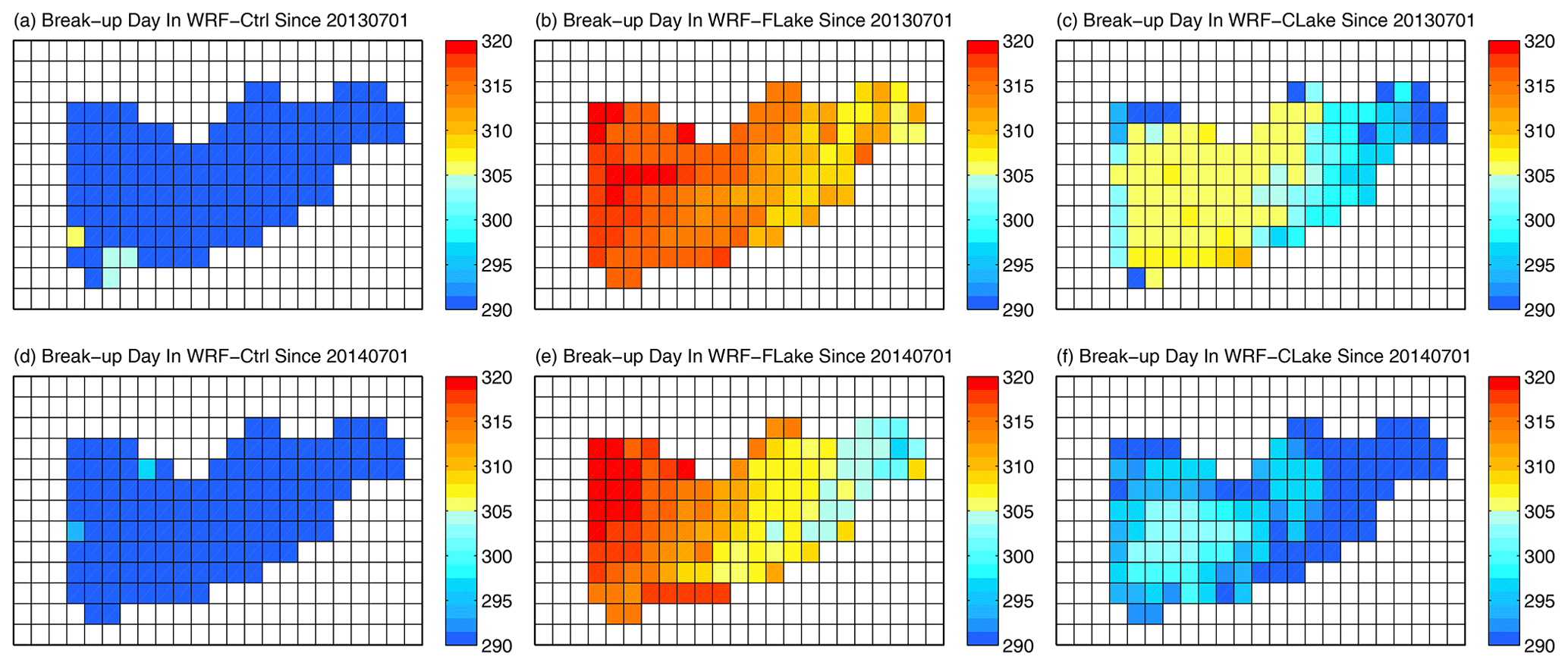
Figure 9 Spatial distribution of the break-up date at Nam Co in each simulation in the spring of (a–c) 2014 and (d–f) 2015. The colour indicates the number of days since 1 July.

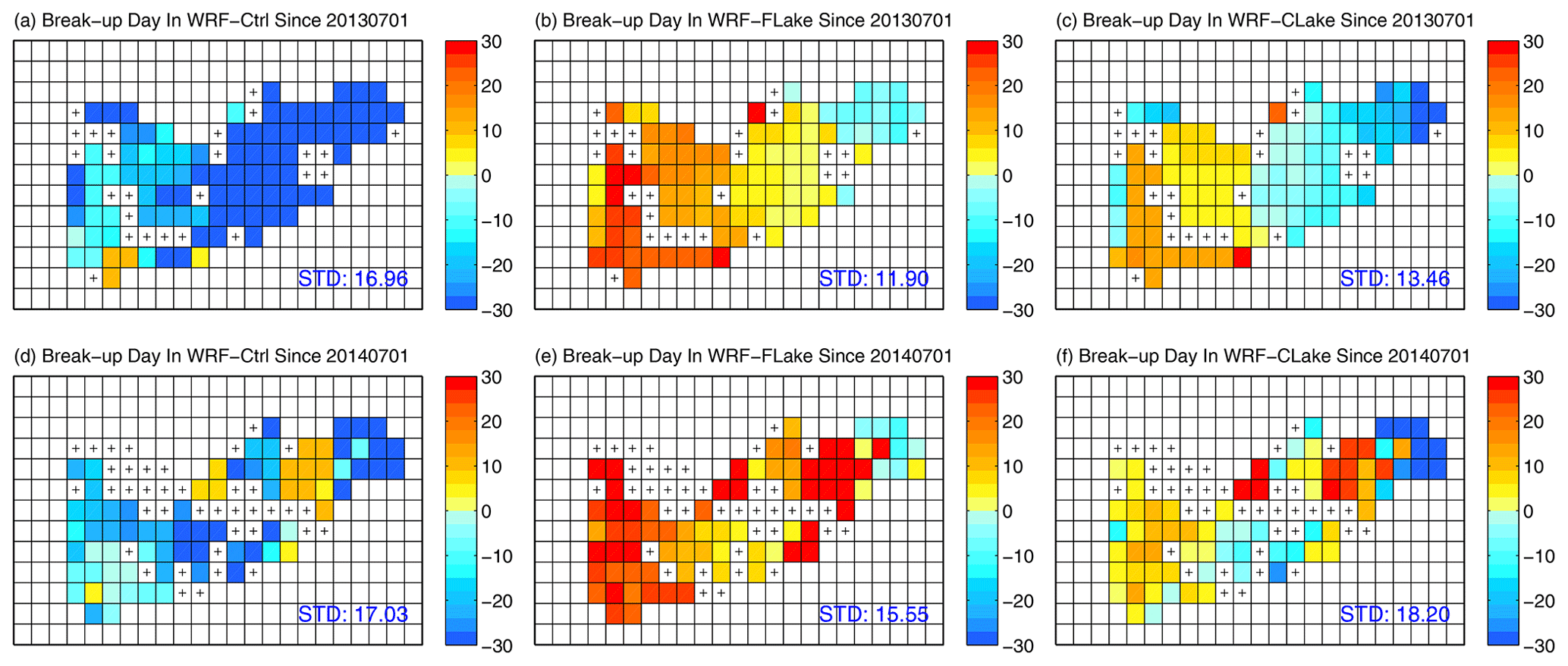
Figure 10 Spatial distribution of biases (days) in break-up date at Nam Co in each simulation in the spring of (a–c) 2014 and (d–f) 2015. The colour indicates the number of days since 1 July. The biases are derived from WRF–Ctrl, WRF–FLake, and WRF–CLake runs minus MODIS. The cross marks denote lake grid points with missing observations in MODIS.

Figure 11 shows the spatial distribution of the freeze-up duration simulated by the two models. All models predicted the longest ice duration in mid-western Nam Co, with WRF–Ctrl having the longest ice duration and WRF–FLake having a slightly longer freeze-up duration than that of WRF–CLake. The differences in the latter two runs could be associated with the differences in the parameterizations of shortwave processes when lake ice exists. Generally, the simulated ice duration is longer than 100 d and shorter than 140 d in both revised models. Figure 12 shows the spatial distribution of biases in freeze-up duration in each simulation. Compared with MODIS, all the models show longer freeze-up durations over the mid-western lake (approximately 10–20 d) and shorter freeze-up durations over the eastern corner of Nam Co (approximately −20 to 10 d). The freeze-up duration being too long in WRF–Ctrl could be associated with the freeze-up dates being too early, while the freeze-up duration being too long in WRF–FLake and WRF–CLake could be associated with the break-up dates being too late. Generally, the variability in the biases in freeze-up duration (blue text in Fig. 10) is much higher than the variability in the biases in freeze-up date and break-up date, which is obviously due to more missing values in MODIS when subtracting the two.

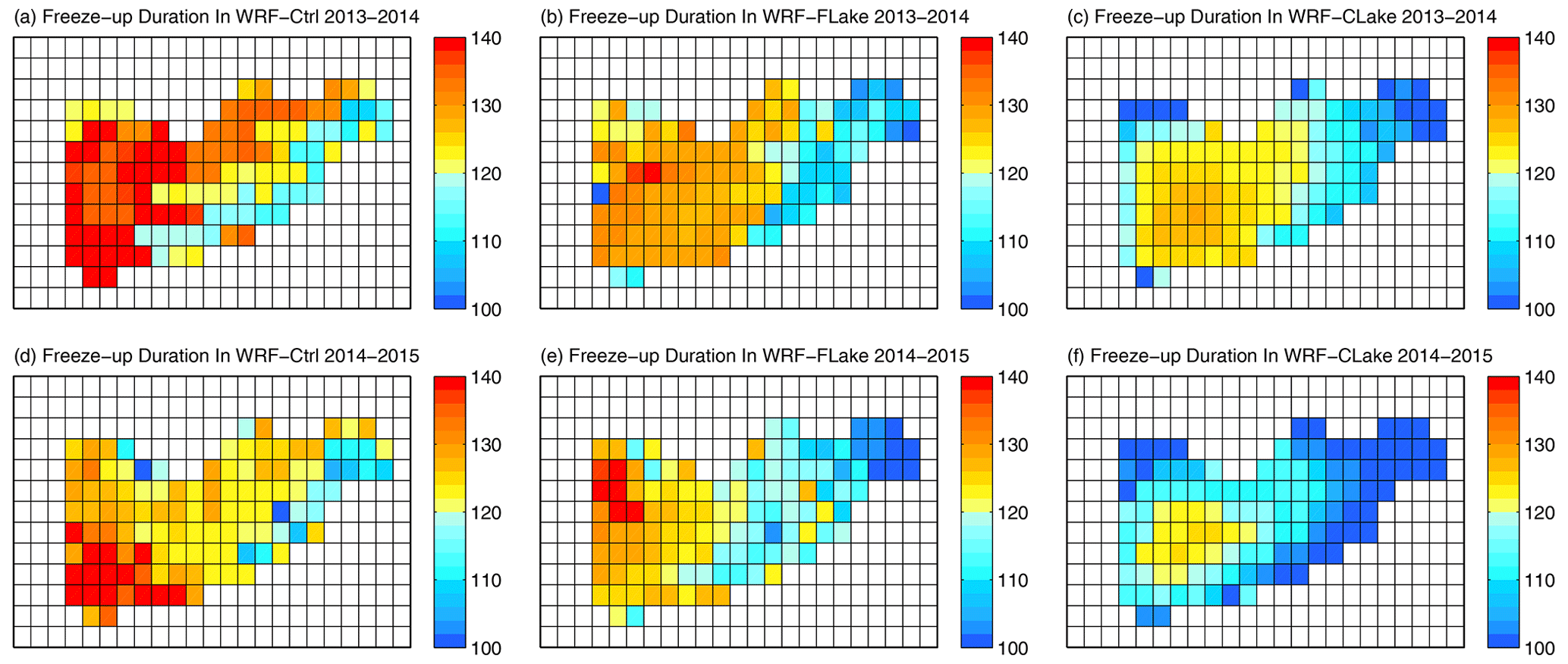
Figure 11 Spatial distribution of the freeze-up duration in each simulation in the periods of (a–c) 2013–2014 and (d–f) 2014–2015. The colour indicates the number of days during freeze-up.

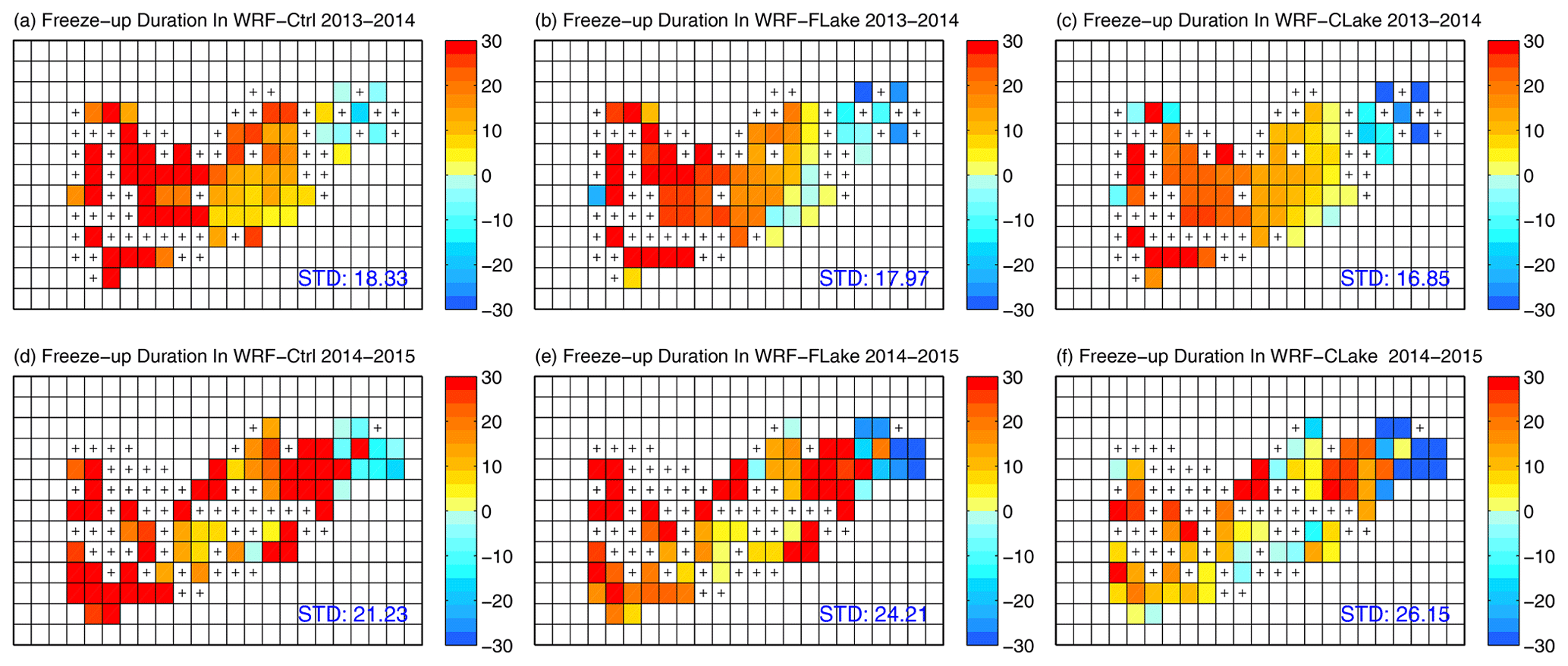
Figure 12 Spatial distribution of biases (days) in freeze-up duration in each simulation in the periods of (a–c) 2013–2014 and (d–f) 2014–2015. The colour indicates the number of days during freeze-up. The biases are derived from WRF–Ctrl, WRF–FLake, and WRF–CLake runs minus MODIS. The cross marks denote lake grid points with missing observations in MODIS.

5 Discussion

The above evaluations demonstrate that with revisions of key parameters and improvements of key parameterizations, associated with surface turbulent heat fluxes during ice-free periods and associated with solar radiation transfer during ice-on periods, the updated model versions can significantly improve the simulation of ice phenology through a better representation of lake energy processes. These improvements are observation and physics based, which is more reasonable and more universal than using an artificial scaling method (i.e. when calculating the sensible heat and latent heat, multiply by a constant) as in Zhou et al. (2023). For example, the WRF–FLake and WRF–CLake models are improved by the same parameterization of water surface roughness length, demonstrating the universality of this scheme as described in Eqs. (4)–(5). Therefore, the current work provides a better model version for weather and climate simulations over alpine lake regions. Nevertheless, there might still be large uncertainties caused by the limitations of models' abilities in depicting some physical processes, which are discussed in this section.

For the freeze-up date, in both periods in 2013–2014 and 2014–2015, MODIS shows early freeze-up in the east of Nam Co (Fig. 6a, d), while the models show early freeze-up in the mid-western lake (Fig. 7). The identical lake depth inevitably causes uncertainties in simulating the freeze-up date. Shallow-water grid points freeze up earlier than deep-water grid points due to less water and lower heat capacity per unit area. Essentially, both lake models are one-dimensional models, and thus we speculate that the mismatch between the model and observation might also be associated with the lake water circulation that cannot be represented in the one-dimensional lake models. In cold seasons, the TP is dominated by prevailing westerlies. Before freeze-up, the wind blowing effect may lead to cool surface water moving to the east and warm deep water moving to the west. A three-dimensional lake model is expected to solve this problem by depicting the horizontal lake water circulation as demonstrated in previous studies (White et al., 2012; Wu et al., 2021). Nevertheless, a one-dimensional lake model is still commonly used in climate models when simulating atmosphere–lake processes, such as the widely used CESM (Oleson et al., 2010) and COSMO (Steppeler et al., 2003), which highlights the importance of the current work.

For the break-up date, in both periods in 2013–2014 and 2014–2015, MODIS shows early break-up in the west (Fig. 6b, e), while the models show early break-up in eastern Nam Co (Fig. 9). The freeze-up time in the models may play a role because early freeze-up grid points may accumulate thicker ice and vice versa for late freeze-up grid points. Additionally, uncertainties associated with snow cover at the lake ice surface play an important role through shortwave-albedo processes, as highlighted by Li et al. (2018) for offline models. In the simulations, there is nearly no snow cover (not shown). However, Fig. 13a and b show that a considerable amount of snow covers the lake surface with inhomogeneous distribution from the west to the east of Nam Co when looking at the images from the Earth Observing System Data and Information System (EOSDIS). Nearly no snow covers the west, and a considerable amount of snow exists over the east. More snow can lead to a high albedo and less shortwave absorption at the surface and can thus have a cooling effect, which will delay ice melting. This contrast in snow cover between the model and observations is consistent and may partly explain the contrast in the spatial patterns of the lake break-up date over Nam Co. In the simulations, nearly no precipitation and snow cover are predicted over the lake ice during freeze-up (not shown). Frozen and smooth surfaces are not favourable for triggering atmospheric convection and snowfall. Therefore, we speculate that the snow cover at the lake ice surface, as shown in the sky view images, might be associated with grid-scale snow dynamic processes like blowing snow during snowfall (as snowflake descent) and after snowfall (at land/lake surface). Previous studies have also demonstrated that snow redistribution by wind and associated changes in depth and density of the snowpack contribute to variations in ice thickness (Brown and Duguay, 2010, 2011). With rough surfaces such as bare ground or vegetated land, the scale of blowing snow might be limited to a small scale and can be parameterized by a scheme such as the one introduced by Xie et al. (2019). In contrast, for a smooth surface, such as the ice surface in the current work, the scale of blowing snow can be much larger. However, such processes are not included in the model version used in current study, and the applicability of such a scheme needs to be further investigated. Furthermore, lakes generally have lower elevations than the surrounding land and are beneficial for snow accumulation, especially during snowfall. Noting that the accurate simulation of precipitation over the complex terrain has long been a challenging issue – i.e. the precipitation in TP can be overestimated by more than 50 % in climate models and even reanalysis data (Gao et al., 2015; Su et al., 2013) – the snowfall simulated over lake will also introduce large uncertainties in modelling the lake surface albedo and thus can influence the lake ice phenology as also demonstrated in a previous study over high-latitude lakes (Fujisaki-Manome et al., 2020).

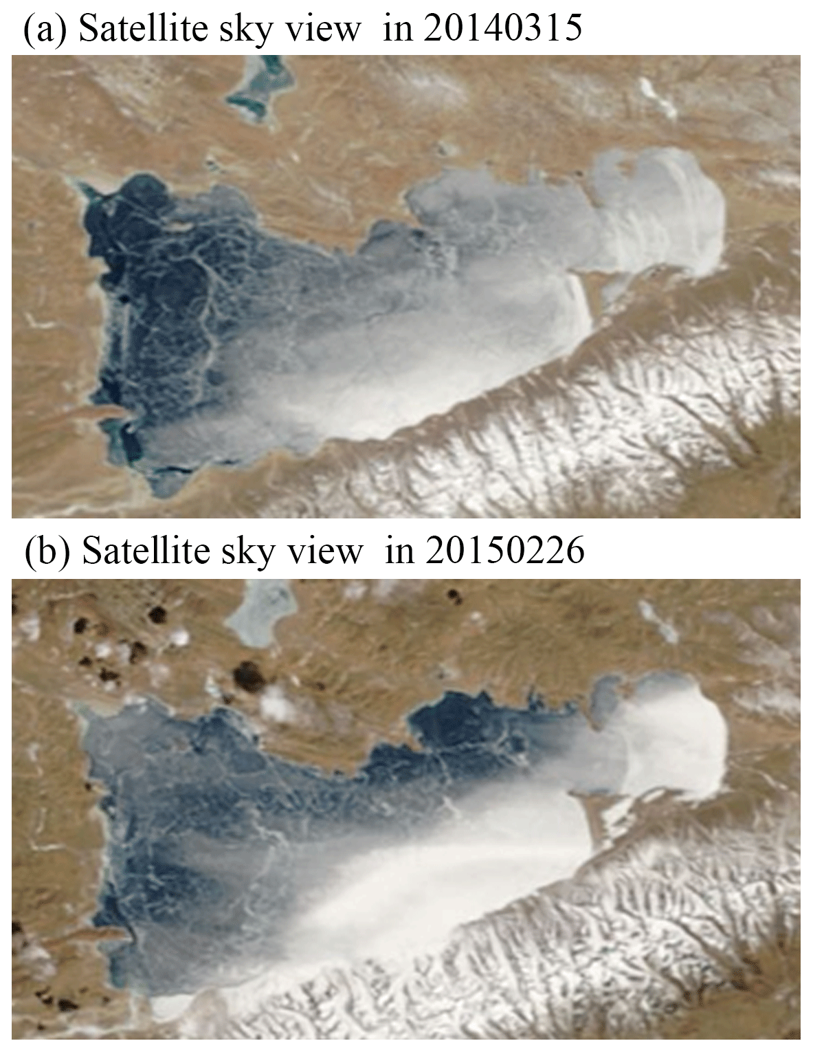
Figure 13 Satellite sky view images from EOSDIS Worldview on typical lake ice-on days in (a) 15 March 2014 and (b)  26 February 2015 (right).

Additionally, other lake processes can also introduce uncertainties in simulating the lake ice phenology. For example, during ice-covered periods, the shortwave radiation absorbed by lake water under ice can increase the water temperature to more than the freezing point (Kirillin et al., 2021; Lazhu et al., 2021; Wang et al., 2022) and delay ice melting by temporarily storing the energy in water instead of being used immediately for ice melting. These uncertainties in describing lake-related processes introduce considerable inconsistencies between models and observations associated with ice phenology. Simultaneously, they also bring great challenges in model applications and developments, especially for deep-alpine-lake regions.

6 Summary and remarks

In this study, the WRF model coupled with two lake models, the FLake model and the default simplified CLM lake model (namely WRF–FLake and WRF–CLake, respectively), was applied to simulate lake ice phenology in a typical alpine lake located in the central TP. With improvements of momentum, hydraulic, and thermal roughness length parameterizations, the WRF–FLake and the WRF–CLake models reasonably simulated the lake water temperature compared with MODIS and station observations. Water temperature represents the lake energy storage, and, therefore, the lake freeze-up date in both models was reasonably simulated compared with MODIS. With improvements of key parameterizations associated with the shortwave radiation transfer, the WRF–FLake and the WRF–CLake models generally simulated the lake break-up date well. Compared with WRF coupled with the default lake model, the simulation of lake ice phenology was significantly improved by WRF coupled to both of the improved lake models. Therefore, we expect that the main results and findings of this work can provide a good reference when simulating lake ice phenology with climate models, especially for the alpine lake.

However, considerable errors still exist in simulating the spatial patterns of freeze-up and break-up dates. These errors could come from the disadvantages of the model in representing some key lake physics such as nonuniform lake depth, lake water circulation, shortwave heating effect on water underneath lake ice, and atmospheric processes such as grid-scale blowing snow, indicating that more substantial work is required to improve the lake physical processes in climate models. Nevertheless, our work can provide a better model version compared with the default WRF model, and the final discussions can provide new implications for improving lake-ice-associated processes in coupled atmosphere–lake models in the future.