Propagating meteorological uncertainty in physically based mountain snow modeling

Snow estimation in mountainous regions is uncertain because meteorology varies with topography, observations are sparse and biased, and snow models are affected by structural and scale limitations. Probabilistic methods are increasingly recognized as essential for quantifying and propagating these uncertainties in hydrological assessment. This study generates meteorological forcing ensembles designed for mountainous terrain and applies them for physically based snow modeling. Precipitation from global station datasets is corrected for wind-induced gauge undercatch using standardized transfer functions. Using geospatial probabilistic estimation, station observations are combined with static topographic predictors and dynamic atmospheric predictors from reanalyses. Deterministic fields are estimated using locally weighted regression and random forests, while spatially correlated random fields sample residuals to produce skillful, reliable ensembles. The resulting ensembles drive the SUMMA energy-balance snow and hydrological modeling framework, calibrated using a Large Sample Emulator approach and applied in three contrasting basins: the Chena (Interior Alaska), Bow (Canadian Rockies), and Tuolumne (Sierra Nevada). Undercatch correction improves cold-season precipitation, dynamic predictors enhance regression skill, and random forests outperform locally weighted regression. Ensemble verification yields positive Brier Skill Scores, and ensemble-forced SUMMA simulations reproduce observed snow water equivalent with realistic magnitude, timing, and uncertainty. This approach advances mountain snow estimation by explicitly representing forcing uncertainty in complex terrain, supporting physically based modeling, data assimilation, and water resource management.

1 Introduction

Measurements and model estimates of mountain snow are essential for predicting runoff, managing flood risk, and planning for water scarcity in snow-dependent regions (Huning and AghaKouchak, 2020; Immerzeel et al., 2020; Sturm et al., 2017; Wood and Lettenmaier, 2008). However, despite the recognized benefits and concerted research efforts, quantifying mountain snow continues to be a persistent challenge characterized by considerable uncertainty (Girotto et al., 2020; Largeron et al., 2020; Dozier et al., 2016). This challenge is driven by the influence of complex terrain on meteorology, snow distribution, and the inability to obtain observations that are spatially and temporally representative (Clark et al., 2011; Frei and Isotta, 2019). Snow models forced with meteorological data are also uncertain, as coarse-scale representations of both meteorology and snow dynamics fail to capture actual snowpack variability (Marsh et al., 2024). The observations used to evaluate and constrain models are typically limited in spatial density and temporal frequency relative to the processes governing snow accumulation and melt (Sturm et al., 2010; Miller et al., 2022; Blöschl and Sivapalan, 1995). Consequently, uncertainty in mountain snow estimation remains substantial and is rarely quantified explicitly.

Estimating meteorological variables in complex terrain has traditionally relied on interpolating sparse station observations into gridded fields while accounting for topographic effects. Early approaches focused on physiographic interpolation, using elevation and terrain descriptors to adjust station data for lapse rates and orographic gradients (Daly et al., 1994; Clark and Slater, 2006). Products such as the Parameter-elevation Regression on Independent Slopes Model (PRISM) follow this framework, combining station observations with expert-based weighting to represent climate fields in mountains (Daly et al., 2008, 2021). Complementary statistical approaches, including locally weighted regression, capture relationships between meteorological variables and static predictors such as elevation, slope, and aspect (Newman et al., 2020). Machine learning (ML) methods such as Random Forests (RF) have also been successfully applied to resolve patterns of meteorological data in complex terrain (Wolfensberger et al., 2021; Baez-Villanueva et al., 2020). However, accurately resolving such variability requires far denser observational networks than currently exist (Frei and Isotta, 2019). Global reanalyses offer consistency and coverage, but they often underperform in complex terrain and require bias correction and down-scaling before hydrological use (Beck et al., 2017; Hong et al., 2022; Berg et al., 2024; Lussana et al., 2018). Deterministic gridded products can overly smooth spatial variability and underestimate extremes (Ensor and Robeson, 2008; Gervais et al., 2014). Gridded meteorological datasets are widely used in snow modeling, but can exhibit substantial bias and lack explicit uncertainty characterization, particularly in mountainous regions (Daly et al., 2021; Henn et al., 2018a). These biases propagate through snowpack simulations, making meteorological forcing a dominant source of model uncertainty (Raleigh et al., 2015; Günther et al., 2019).

Snow observations are essential for understanding snowpack evolution and constraining models, but remain limited in spatial and temporal coverage. In situ networks, including snow pillows, automated sensors, and manual surveys, provide locally accurate estimates of snow depth and water equivalent, but are too sparse to capture heterogeneity driven by topography, wind, and vegetation (Pomeroy et al., 2007; Brown et al., 2019; Mortimer and Vionnet, 2025a; Clark et al., 2011). Airborne and terrestrial lidar, along with satellite remote sensing, have expanded the ability to map high resolution snow depth, cover, and albedo across larger domains (Deems et al., 2013; Painter et al., 2016; Gascoin et al., 2024). However, their use remains constrained by infrequent coverage, uncertainties in converting depth to water equivalent, and retrieval challenges in forested or complex terrain (Sturm et al., 2010; Margulis et al., 2019). Reanalysis and remote-sensing products complement ground-based observations by providing spatially continuous fields where in situ measurements are sparse or unreliable, however they also contain errors and biases (Lundquist et al., 2019; Stillinger et al., 2023).

Snow models are widely used to quantify snow mass, codify process understanding and support hydrologic prediction (Pomeroy et al., 2007; Vionnet et al., 2021a; Essery et al., 2013; Sun et al., 2019; Marsh et al., 2024). Approaches range from lumped conceptual degree-day models to physically based, high-resolution systems that resolve energy balance, blowing snow, canopy interception, and avalanching (Hrachowitz and Clark, 2017; Magnusson et al., 2015). However, increased model complexity does not necessarily improve predictive performance, and meteorological forcing, structural and parameter uncertainties often dominate and compensate for unresolved processes (Menard et al., 2021). Model Intercomparison Projects (MIPs) demonstrate that inter-model variability arises not only from differing process representations but also from forcing data, calibration, and scale mismatches (Essery et al., 2013; Menard et al., 2021). Modeling in complex terrain presents distinct challenges, including steep energy-balance gradients, heterogeneous snow processes, and systematically biased precipitation inputs (Zhao and Li, 2015; Clark et al., 2011). Key processes such as refreezing, sublimation, wind redistribution, and rain-on-snow thermodynamics remain difficult to accurately simulate, yet strongly influence snow mass and energy budgets (Marks et al., 1998; Pomeroy et al., 2016; Barlage et al., 2010). As a result, snow model uncertainty reflects both incomplete process understanding and the difficulty in parameterizing subgrid variability in meteorological and terrain drivers (Günther et al., 2019). Increasingly, ensemble modeling, data assimilation, and high-resolution process studies are being used to constrain model states and improve predictive skill (Girotto et al., 2020; Largeron et al., 2020; Vionnet et al., 2021a; Sun and Margulis, 2026; Mott et al., 2023).

Ensemble approaches provide a means to represent and propagate uncertainty in both model inputs and model states. In meteorology and climate science, ensembles are used to characterize distributions of plausible outcomes (Collins, 2007), and hydrology has increasingly adopted ensemble methods to quantify predictive uncertainty and provide probabilistic streamflow forecasts (Cloke and Pappenberger, 2009; Wu et al., 2020). In mountain environments, where predictive skill depends critically on accurate representation of snowpack states, ensemble methods enable data assimilation to integrate observations to improve snow estimation (Clark et al., 2006; Wood et al., 2016; Vernay et al., 2015; Largeron et al., 2020; Girotto et al., 2020). Recent developments in meteorological ensembles that incorporate both static topographic controls on observations and dynamic atmospheric predictors offer promising pathways for capturing input uncertainty (Clark and Slater, 2006; Newman et al., 2020; Bunn et al., 2022; Tang et al., 2024). Better characterization of precipitation and temperature uncertainty is particularly important, for example, given the increasing frequency of rain-on-snow events under a warming climate (Hotovy et al., 2025; Musselman et al., 2018). This evolution from deterministic interpolation to probabilistic ensemble generation reflects a growing recognition that uncertainty quantification is essential in mountainous terrain (Frei and Isotta, 2019; Bertoncini and Pomeroy, 2025; Kim et al., 2021; Mott et al., 2023).

A key gap remains in how probabilistic meteorological information is generated and evaluated for mountain snow modeling. Most existing studies in complex terrain focus on developing or validating probabilistic precipitation and temperature estimates (e.g., Frei and Isotta, 2019; Bertoncini and Pomeroy, 2025), yet few extend this uncertainty representation through to physically based snow modeling. Consequently, the influence of forcing uncertainty on simulated snowpack evolution, melt timing, and water availability remains poorly quantified (Dozier et al., 2016; Largeron et al., 2020; Girotto et al., 2020; Tang et al., 2025a). Mountain snow modeling studies using physically based or energy-balance approaches very often continue to rely on a single deterministic meteorological forcing, typically derived from gridded observation-based or downscaled reanalysis products (Essery et al., 2013; Vionnet et al., 2021a; Berg et al., 2024; Marsh et al., 2024). Many studies evaluating snow ensembles have used “ensembles of opportunity” assembled from independent reanalysis datasets, which capture the diversity of datasets but not the true uncertainty (Schreiner-McGraw and Ajami, 2022; Henn et al., 2018b; Kim et al., 2021; Tyson et al., 2023; Casson et al., 2018). There is therefore a need for approaches that explicitly represent meteorological uncertainty and propagate it through physically based snow models.

This study addresses this need by linking station-based probabilistic meteorology with physically based snow modeling. The workflow explicitly corrects for precipitation undercatch, generates spatially and temporally coherent high-resolution meteorological ensembles, and propagates these uncertainties through the SUMMA energy-balance snow model. By testing this approach across three contrasting mountain basins, the Chena (Interior Alaska), Bow (Canadian Rockies), and Tuolumne (Sierra Nevada), using large domain datasets, this study demonstrates a transferable approach for representing and evaluating forcing uncertainty through to physically based snow modeling in complex terrain. The remainder of this paper is structured as follows. Section 2 describes the study areas and river basins. Section 3 describes the datasets used to construct and evaluate the ensembles and snow simulations. Section 4 describes the ensemble forcing methodology, including undercatch correction, predictor screening, and ensemble generation using a geospatial probabilistic estimation approach, followed by the physically based modeling. Section 5 presents the evaluation of the ensemble meteorology and snow simulation in the three basins. Section 6 discusses the implications of constructing mountain meteorological ensembles and snow modeling, and Sect. 7 summarizes key findings and future directions.

2 Study Area

Three river basins were selected to represent a broad range of hydroclimatic, physiographic, and monitoring contexts: the Chena above Two Rivers (Alaska), the Bow above Calgary (Alberta), and the Tuolumne above Hetch Hetchy (California) (hereafter Chena, Bow, and Tuolumne; Fig. 1). Snow observation datasets in the basins have comparable station densities; however, they differ in meteorological observational networks, climate regime, and hydrological landscape. These contrasts encompass subarctic, continental mountain, and maritime-influenced high-elevation environments. Together, these basins provide a set of testbeds that capture the diversity of conditions under which ensemble meteorological forcing systems for mountainous snow modeling must operate.

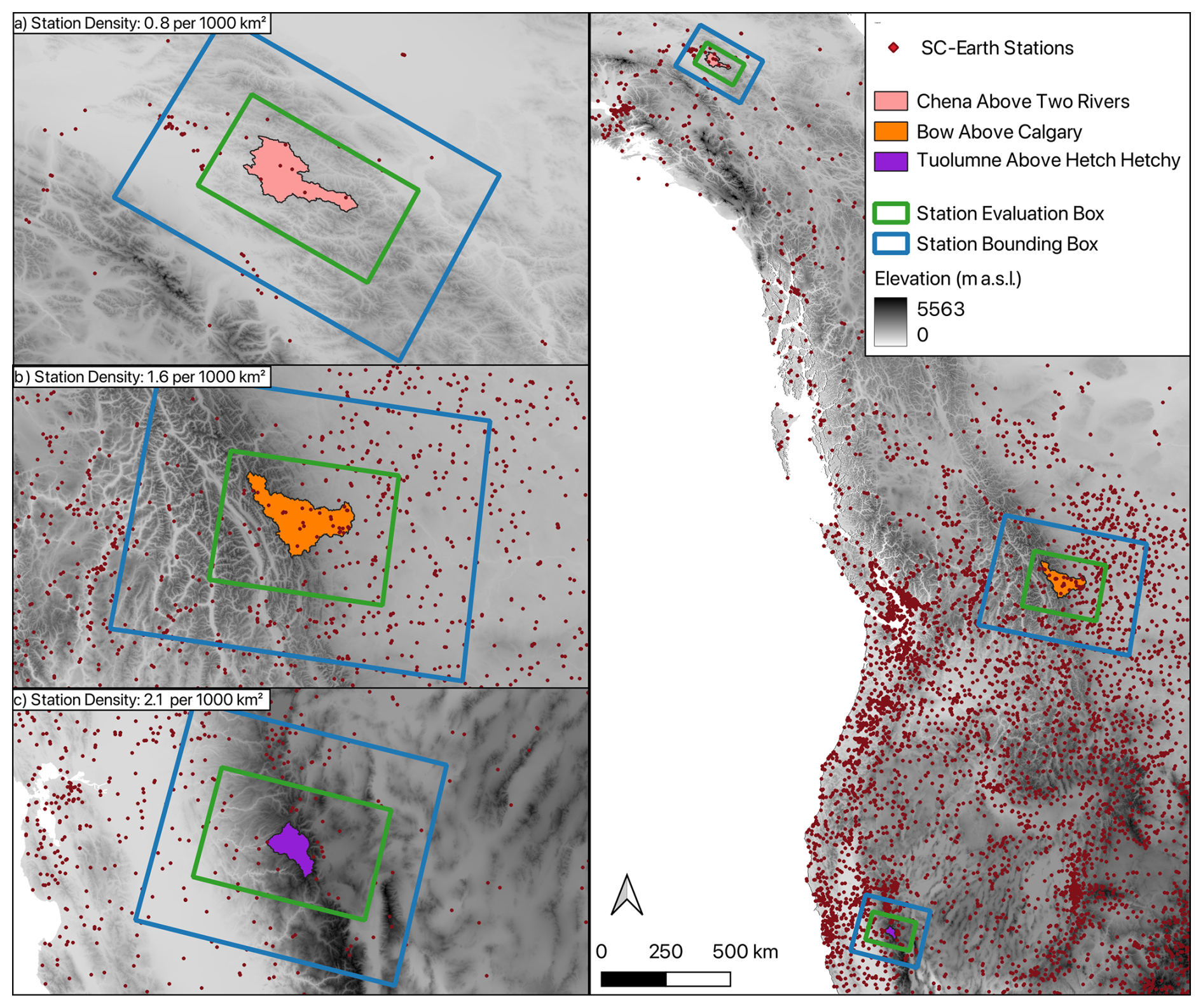
Figure 1 Chena, Bow, and Tuolumne river basins shown with SC-Earth meteorological stations. The larger station bounding box (blue) delineates the stations used to build ensembles and the area for grid generation. The smaller station evaluation box (green) delineates the stations used to evaluate meteorological ensemble performance. The elevation is shown as meters above sea level ($\mathrm{m}\mathrm{a}.\mathrm{s}.\mathrm{l}.$) from MERIT Hydro.

The Chena is a tributary of the Tanana River in Interior Alaska, flowing westward towards Fairbanks. The Chena originates in the Yukon-Tanana Uplands, a region of rolling hills and mountains, with vegetation characterized by a mixture of boreal forest and permafrost (Frey et al., 1970; Anderson, 1970). The basin covers an area of approximately 5500 km², with an elevation ranging from approximately 100 $\mathrm{m}\mathrm{a}.\mathrm{s}.\mathrm{l}.$ at the outlet to 1600 $\mathrm{m}\mathrm{a}.\mathrm{s}.\mathrm{l}.$ at its highest point (Daly and Vuyovich, 2012). It contains discontinuous permafrost, with the highest concentrations occurring at higher elevations. The watershed experiences a subarctic climate, characterized by cold, dry winters and warm, relatively humid summers. Annual precipitation averages 380 to 510 mm yr⁻¹ and basin hydrology is dominated by snowmelt runoff, though the largest recorded floods have occurred in summer due to intense rainfall (Liao and Zhuang, 2017). Snow observations in the Chena region are challenging due to difficulties in accurately measuring solid precipitation and the sparse distribution of observation stations across a large terrain (Bennett et al., 2019). Due to previous flood events, infrastructure developments and location above Fairbanks, there are dedicated snow monitoring stations and programs in the Chena. The majority of snow monitoring stations are part of the Natural Resources Conservation Service (NRCS) Snow Telemetry (SNOTEL) program (Fleming et al., 2023). The NRCS also conducts snow surveys twice per year at the start of April and May at several locations throughout the basin (Daly and Vuyovich, 2012).

The Bow is located in the Eastern Canadian Rocky Mountains in Southern Alberta. It flows south-east through Banff National Park and the foothills, then meanders eastward through the Prairies towards its confluence with the Oldman River (Tanzeeba and Gan, 2012). The Bow basin covers approximately 25 000 km² and begins at Bow Lake at 1920 $\mathrm{m}\mathrm{a}.\mathrm{s}.\mathrm{l}.$, then drops to 1180 $\mathrm{m}\mathrm{a}.\mathrm{s}.\mathrm{l}.$ at its confluence with the Oldman River (BRCB, 2010). The Bow has a semi-arid climate with precipitation of roughly 400–500 mm yr⁻¹. Snowmelt runoff accounts for roughly 80 % of the Bow River inflow, the rest coming from rainfall, groundwater, and a small (3 %) contribution from glacier melt (Bash and Marshall, 2014). The mountainous regions of the watershed are a dominant source of surface water, and exert control over flood-to-drought conditions (Vionnet et al., 2020). Snow monitoring in the Bow combines automated sites and manual snow surveys focused on late winter (Vionnet et al., 2020).

The Tuolumne is located in the Sierra Nevada in California and flows from high-elevation headwaters in Yosemite National Park to its confluence with the San Joaquin River. The Tuolumne spans 700–3900 $\mathrm{m}\mathrm{a}.\mathrm{s}.\mathrm{l}.$ in elevation, covering approximately 1650 km². Tuolumne streamflow is primarily driven by seasonal snowmelt, supporting downstream ecosystems, agriculture, and urban water supplies. Approximately 80 %–90 % of the annual precipitation (800–1000 mm yr⁻¹) occurs as snow during winter months, though both precipitation amount and timing show considerable seasonal and year-to-year variability (Cristea et al., 2014). The Tuolumne Above Hetch Hetchy has low human intervention, such as dams or diversions, and land-use changes (Rice et al., 2011). The snow distribution in the Tuolumne River Basin is relatively similar from year to year, mostly controlled by strong topography and similar storm tracks controlling snow deposition patterns (Pflug and Lundquist, 2020; Lundquist et al., 2015a). The Tuolumne has been extensively studied for snow distribution due to its importance for water supply and the availability of high-resolution snow-depth measurements from airborne lidar (Painter et al., 2016). The combination of scanning lidar, an imaging spectrometer, and physically based modeling has produced a unique dataset of high-resolution snow water equivalent and snow albedo maps. These spatially detailed data have led to numerous studies assessing snow quantity and distribution (Margulis et al., 2019; Currier and Lundquist, 2018; Pflug and Lundquist, 2020), as well as water balance and runoff estimation (Lundquist et al., 2015b; Henn et al., 2016, 2018c; Hedrick et al., 2020).

3 Data

All datasets used in this study were selected and processed in accordance with FAIR data principles (Wilkinson et al., 2016). The analysis integrates publicly available meteorological, topographic, and snow observation datasets, each documented with open metadata and standardized formats to promote transparency and interoperability.

3.1 Meteorological Station Data

This study uses a Serially Complete (SC) station dataset that includes daily precipitation, mean temperature, temperature range and wind speed with global spatial coverage from 1950–2019 (Tang et al., 2021). This SC-Earth station dataset is derived primarily from raw data from the Global Historical Climatology Network–Daily (GHCN-D; Durre et al., 2010) and the Global Surface Summary of the Day (GSOD; Menne et al., 2012). ERA5 reanalysis data are also used in SC-Earth production to correct a timeshift issue and assist with global gap filling. GHCN-D has been widely used for the production, evaluation, and correction of gridded meteorological datasets (Contractor et al., 2020; Beck et al., 2017; Hong et al., 2022; Tang et al., 2020). It includes precipitation and temperature data that undergo a comprehensive, automated quality assurance process (Durre et al., 2010). GSOD provides complementary wind speed observations used here to implement a precipitation undercatch correction strategy, though its quality control protocols are less rigorous, and caution is advised when using GSOD and SC-Earth wind estimates (Tang et al., 2021). GHCN-D, GSOD, and SC-Earth datasets do not include undercatch adjustments.

Station data compiled in SC-Earth originate from diverse networks employing various gauge configurations. In the Bow watershed, for instance, multiple monitoring networks use different gauge types even within the same region (Bertoncini and Pomeroy, 2025). Across the Chena, Bow, and Tuolumne basins, meteorological observations come from numerous providers lacking detailed gauge metadata. Although additional research datasets exist for these basins, they were not examined in this study due to limited temporal coverage, study-specific assumptions and lack of serial completeness (Daly and Vuyovich, 2012; Fang et al., 2019; Lundquist et al., 2016; Henn et al., 2016; Bertoncini and Pomeroy, 2025).

3.2 Topographic and Land Surface Data

The MERIT Digital Elevation Model (DEM) is used for multiple applications in this study, including the derivation of topographic descriptors for geospatial estimation. MERIT DEM is available globally at 3 arcsec (90 m at the equator) horizontal resolution (Yamazaki et al., 2017). In a previous study using the geospatial probabilistic estimation methodology, descriptors such as elevation, latitude, longitude, and west-east and south-north slopes (which proxy for terrain aspect) were utilized (Newman et al., 2015). This current study assesses these predictors, and also examines aspect, slope, and topographic position index (TPI). Topographic predictors were also smoothed with a two dimensional Gaussian filter over different radii to evaluate the relative skill as a regression predictor.

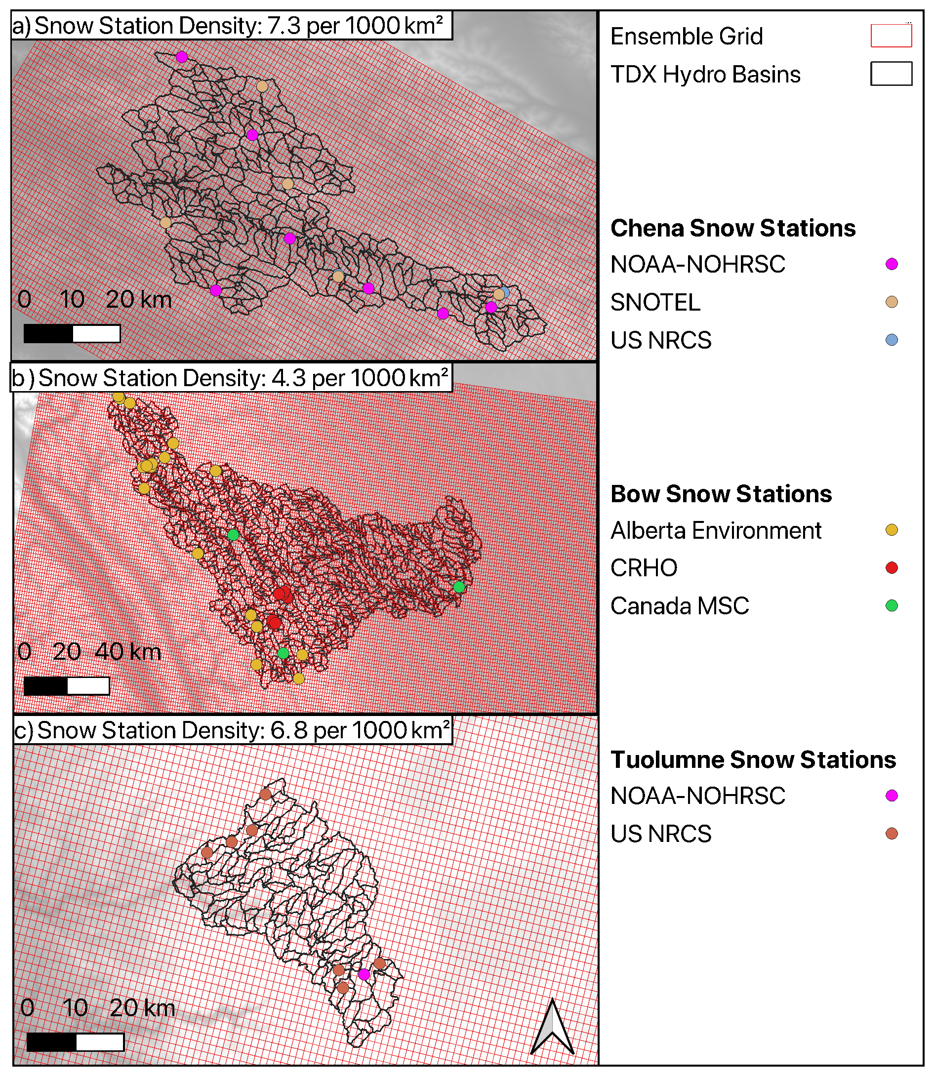
Figure 2 Chena, Bow, and Tuolumne River Basins showing the meteorological forcing grid ($\mathrm{1}/\mathrm{64}$°) in red, the TDX Hydro basin delineations in black, and the snow stations from the multi-source NorSWE dataset. Data sources include National Oceanic and Atmospheric Administration – National Operational Hydrologic Remote Sensing Center (NOAA-NOHRSC), SNOwpack TELemetry Network (SNOTEL), United States Natural Resources Conservation Service (US NRCS), Canadian Rockies Hydrological Observatory (CRHO) and Canada Meteorological Services of Canada (Canada MSC). The NRCS data sources compile observations from state level collection offices, including California Department of Water Resources.

TanDEM-X Hydro (TDX-Hydro), a catchment and vector stream network dataset, was used for the spatial discretization of the hydrological model, as shown in Fig. 2. This dataset was derived from high-resolution (12 m) TanDEM-X elevation data conditioned with vegetation bias removal, adaptive smoothing, river enforcement, and depression handling, resulting in a highly detailed representation of global hydrography (Carlson et al., 2024). The underlying TanDEM-X elevation data are not publicly available, however TDX-Hydro discretizations are. The use of a high-resolution catchment dataset helps capture topographic details such as elevation more accurately. Working with smaller catchments, the dataset can capture terrain variations that coarser datasets might miss; however, there is a trade off between spatial resolution and computational time in modeling (Chaney et al., 2018). For consistency between river basins, the discretization approach taken does not explicitly represent some topographic controls on snow, such as slope and aspect.

Multiple geospatial datasets are used to support hydrological model parameterization and the calculation of catchment attributes, including land cover and aspect. Land cover characteristics are obtained from the MODIS MCD12Q1 dataset (Friedl and Sulla-Menashe, 2019), and soil properties are sourced from the USDA NRCS database (Knoben, 2021) derived from the SoilGrids 250 m dataset (Hengl et al., 2017). Further details on these datasets applied for hydrological modeling are available in Knoben et al. (2022).

3.3 In Situ Snow Data

The Northern Hemisphere Historical In Situ Snow Water Equivalent Dataset (NorSWE) provides a comprehensive record of snow water equivalent (SWE) observations spanning 1979–2021 (Mortimer and Vionnet, 2025a). The NorSWE dataset integrates data from nine sources across North America, Russia, and Finland. It includes SWE measurements from manual snow surveys, snow pillows, airborne and ground-based passive gamma radiation sensors, with snow depth (SD) data included when available. Bulk snow density is derived where both SWE and SD are present. Quality control procedures, adapted from (Vionnet et al., 2021b), include variable-specific range checks and elevation verification using the USGS National Elevation Dataset where applicable.

For the calibration of snow parameters using a Large Sample Emulator (LSE) approach, station data from Mortimer and Vionnet (2025a) and Sun et al. (2019) are used. For analysis of the undercatch correction procedures, the quality-controlled dataset of Smith et al. (2022) was used for comparative purposes.

3.4 Remotely Sensed and Lidar Snow Data

Spatial snow cover was characterized using the Moderate Resolution Imaging Spectroradiometer (MODIS) Terra Snow Cover Daily L3 Global 500 m product (MOD10A1, Collection 6.1), which provides daily global snow cover observations derived from the Normalized Difference Snow Index (NDSI) (Hall and Riggs, 2021). The MODIS product was used to derive spatial metrics that describe the extent and seasonal evolution of snow cover.

Spatial snow water equivalent (SWE) estimates were obtained from the Airborne Snow Observatory (ASO) L4 Lidar Snow Water Equivalent 50 m product for the Tuolumne (Painter, 2018). The ASO program combines airborne lidar measurements of snow depth with physically based snow density modeling to produce high-resolution SWE estimates across mountainous watersheds (Painter et al., 2016). These data provide spatially distributed estimates for evaluating simulated SWE patterns.

3.5 Meteorological Reanalyses

The European Centre for Medium-Range Weather Forecasts (ECMWF) Reanalysis v5 (ERA5) is a state of the art global reanalysis dataset that provides consistent and high-quality estimates of atmospheric, land, and oceanic variables from 1950 to the present (Hersbach et al., 2020). In this study, we use ERA5 atmospheric (meteorological) forcing variables from the full reanalysis product, rather than the higher-resolution ERA5-Land dataset. ERA5 combines a vast array of historical observations with advanced numerical weather prediction models through data assimilation techniques to produce a spatial resolution of 0.25° and hourly temporal resolution. In this study, we use wind and temperature from ERA5 for station precipitation undercatch correction when co-located measurement data are not available. Additionally, we use ERA5 as a benchmark forcing dataset for evaluating snow modeling performance within the Structure for Unifying Multiple Modeling Alternatives (SUMMA) hydrological modeling framework (Clark et al., 2015a, c, b).

The Canadian Surface Reanalysis (CaSR) is a high-resolution, observation-constrained reanalysis dataset developed to provide detailed surface meteorological fields over North America (Gasset et al., 2021). The most recent version, CaSR v3.1, incorporates enhancements to the data assimilation system, expanded observational networks, and updated model physics to improve the representation of near-surface atmospheric conditions. CaSR provides meteorological variables at a 10 km spatial resolution and hourly temporal frequency, making it well-suited for regional hydrometeorological studies. In this study, CaSR is used as a source of dynamic predictor data for geospatial estimation and as a benchmark dataset for evaluating snow modeling performance within the SUMMA.

4 Methods

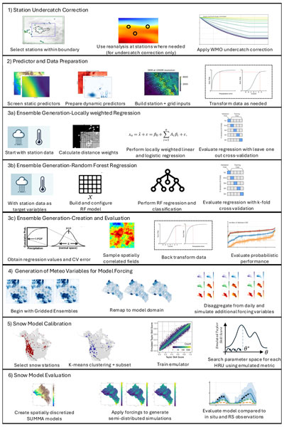
Reproducibility has historically been a challenge in hydrology and water resources research (Stagge et al., 2019). Recent efforts have emphasized open, transparent, and automated workflows in the Earth sciences (e.g., Gil et al., 2016; Knoben et al., 2022; Arnal et al., 2024). This study follows a structured workflow, which is illustrated at a high level in Fig. 3.

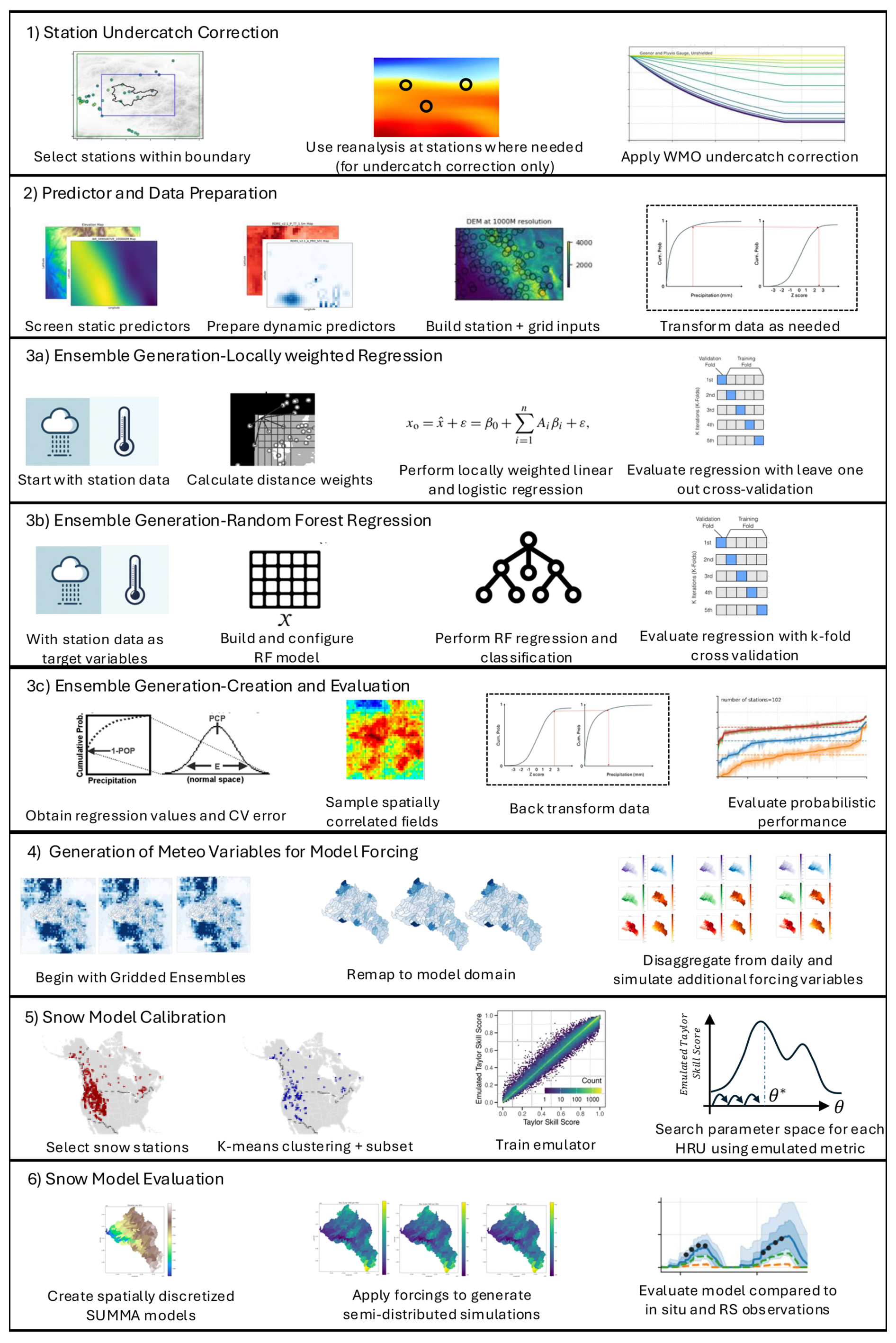
Figure 3 Overview of the Study Methodology. Methods 3–4 are components of the GPEP ensemble forcing generation approach.

The study methodology from data processing to model simulation is implemented with Snakemake workflows (Köster and Rahmann, 2012). Snakemake is a rule based management system that utilizes a Directed Acyclic Graph (DAG) to represent and manage the dependencies within a workflow. This allows reproducibility, transparency, and scalability across computational environments. An example DAG illustrating the workflow structure is provided in the supplementary material.

4.1 Station Undercatch Correction

Undercatch refers to the systematic underestimation of precipitation caused by wind effects, gauge configuration, and precipitation phase, which reduce the fraction of precipitation captured by instruments (Kochendorfer et al., 2017a, b). The bias is most pronounced for solid precipitation in cold and windy environments (Smith et al., 2022; Mekis and Vincent, 2011; Mekis et al., 2018), making undercatch correction an important step when generating precipitation reanalyses and datasets (Newman et al., 2020; Behrangi et al., 2018). A range of approaches exists for correcting undercatch, including empirical wind-based transfer functions, water-balance closure, and computational fluid-dynamics modeling (Colli et al., 2018, 2020; Beck et al., 2019). In this study, we apply empirical, gauge-based correction functions derived in the World Meteorological Organization (WMO) Solid Precipitation Intercomparison studies (Goodison et al., 1998; Kochendorfer et al., 2017b, a). These functions relate catch efficiency (CE) to wind speed and air temperature and are derived specific to gauge types and shielding configurations as shown in Fig. 4.

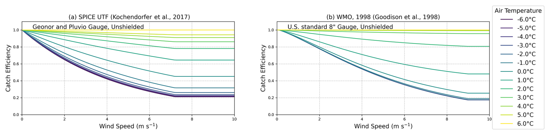
Figure 4 Catch efficiencies for the undercatch correction methods applied in this study based on temperature and wind speed. The updated SPICE UTF Kochendorfer et al. (2017a) to the Bow Basin is shown on the left side (a). On the right side (b) for the Chena and Tuolumne the approach from Goodison et al. (1998) and wind speed threshold behavior from Yang et al. (1998).

A regional approach that assumes consistent gauge type and configuration within each basin is taken. Specifically, in the Bow Basin the WMO SPICE UTF was applied for assumed unshielded Geonor and Pluvio gauges, and in the Chena and Tuolumne the WMO (1998) standard rain gauge correction is applied for assumed unshielded US standard 8-inch gauges (Goodison et al., 1998; Yang et al., 1998; Kochendorfer et al., 2017a, b). This follows a similar methodology to Newman et al. (2020) that derived large-domain station undercatch corrections for Alaska, as well as Huidobro et al. (2023) that made similar assumptions due to lack of consistent gauge metadata across large domains of the United States. As demonstrated by Kochendorfer et al. (2017a) and Pierre et al. (2019), along with the dominant effect of shielding, climate exerts a strong influence on catch efficiency relative to specific instrument type and the robustness of generalized transfer functions. The primary objective is not to compare methods directly, but to implement an appropriate correction for stations in each basin given available information. Due to a lack of station metadata in global datasets and with individual network providers, we assume a single gauge configuration per basin. Gridded reanalysis was used where co-located measurements were not available in an approach similar to Bertoncini and Pomeroy (2025). Wind observations at gauge height are used where available (e.g., GSOD), while ERA5 reanalysis winds translated to gauge height were used to supplement gaps for GHCN-D stations (Yang et al., 1998). ERA5 temperatures, lapsed to station elevation, are used to estimate precipitation phase and apply temperature-dependent correction factors. Full methodological details and equations are provided in Appendix A.

4.2 Predictor and Data Preparation

In complex terrain, such as mountainous environments, topography is an important consideration to determine variables such as precipitation and temperature (Clark and Slater, 2006; Böhner and Antonić, 2009). Elevation impacts temperature through the adiabatic lapse rate, where temperature decreases with altitude (Daly et al., 2008). Precipitation patterns shift at higher elevations due to orographic lifting, leading to increased rainfall on windward slopes and rain shadows on leeward sides (Napoli et al., 2019). Additionally, slope and aspect determine the amount of solar radiation received, affecting localized heating and cooling rates (Böhner and Antonić, 2009). West-East and South-North elevation derivatives (gradients or slopes) capture directional changes in terrain, which can influence wind flow and the distribution of moisture, further impacting weather patterns (Robert et al., 2013).

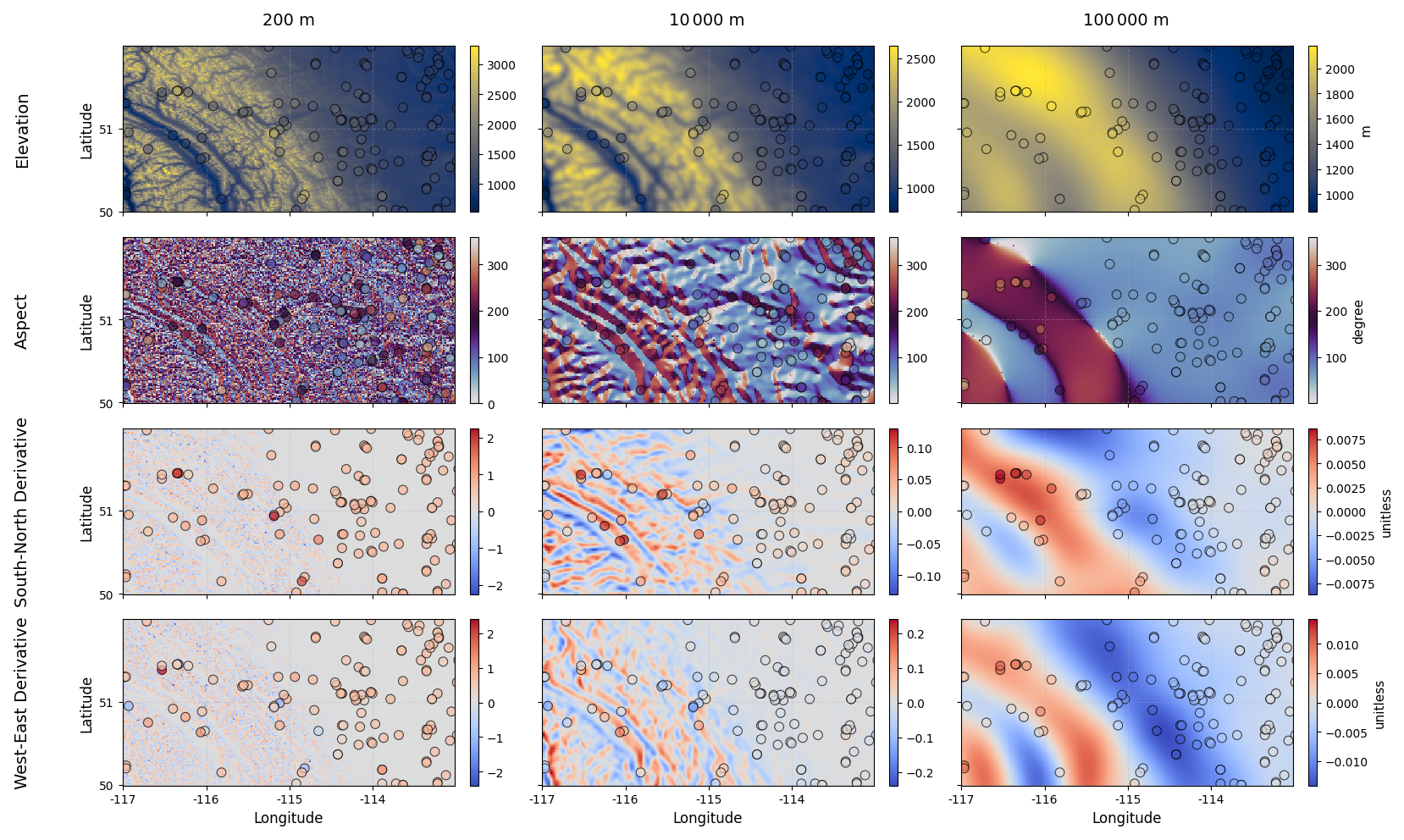
Figure 5 Visual comparison of topographic descriptors used as static predictors in deterministic regression. Calculated based on the MERIT-DEM, and applying a 2D Gaussian filter of varying radii (200, 10 000, and 100 000 m) examples for DEM, Aspect, South-North and West-East Derivatives are shown. Station location and values derived from the gridded products are indicated within the circles.

Topographic descriptors are terrain variables calculated from a DEM to quantify elevation, spatial gradients and patterns. In this study, topographic descriptors derived from MERIT DEM are evaluated and applied as static predictor variables for precipitation and temperature. We compare simple intuitive descriptors of elevation, latitude, and longitude to derived ones, such as directional derivatives, Topographic Position Index (TPI), and aspect. Smoothing of topographic descriptors is performed to reduce noise and emphasize broader trends across the landscape as shown in Fig. 5. This is explicitly examined by applying a 2D Gaussian filter with varying radii (200, 1000, 10 000, 100 000, 150 000 m) to assess skill as a static predictor of precipitation and temperature.

Predictor selection for the regression models used cross-validation error in a sequential forward screening procedure. An initial evaluation of static predictors was conducted to identify an appropriate level of spatial smoothing, after which the static variables were combined through iterative screening. Starting from an empty model, the static predictor producing the highest cross-validated Kling–Gupta Efficiency (KGE^′′) was first selected. Then additional static predictors were added one at a time, each time retaining the variable that yielded the greatest improvement in cross-validated KGE^′′. This process continued until the model skill no longer increased appreciably (defined as a gain in KGE^′′ ≤ 0.01).

Dynamic predictors from gridded reanalysis were subsequently incorporated using the same forward screening procedure. The screening and regression fitting were performed independently for precipitation and temperature, allowing the most relevant static and dynamic predictors to be identified for each variable. The resulting predictor sets for precipitation and temperature were then combined to form the final predictor configuration used in the ensemble generation stage. The dynamic predictors consisted of the seven meteorological forcing variables required to drive the physically based hydrological model as provided in the supplementary material. Precipitation and temperature were the primary variables of interest, while shortwave and longwave radiation, humidity, and wind speed were included to represent spatial variability in energy balance and atmospheric conditions. Together, these variables form the standard meteorological forcing set used in land surface models, ensuring that precipitation and temperature remain physically consistent with broader climatic drivers while maintaining practicality for operational implementation.

4.3 Ensemble Meteorological Forcing Generation

Meteorological datasets that represent spatially distributed meteorological fields are fundamental to hydrology and land-surface modeling. The fidelity of these datasets depends on their ability to capture spatial variability and to characterize associated uncertainties in observation-based estimates. To address this challenge, a probabilistic interpolation framework was first developed by Clark and Slater (2006), who implemented a Locally Weighted Regression (LWR) approach for generating ensembles of daily precipitation and temperature from station observations along with Spatially Correlated Random Fields (SCRF) to produce ensembles from sampling regression residuals. This foundational approach provides a statistical means of estimating both the mean and uncertainty of meteorological fields through spatial regression and stochastic simulation. Newman et al. (2015) refactored this approach into a formal Fortran-based software (the Gridded Meteorological Ensemble Tool, GMET) and produced a 100-member ensemble of daily precipitation and temperature for the contiguous United States (CONUS), demonstrating a practical capability to generate uncertainty-aware large-domain gridded forcings. Newman et al. (2020) applied the framework for Alaska, including station based undercatch based on regional gauge type assumptions. Subsequent enhancements enabled integration with deterministic gridded fields and data assimilation applications, providing dynamic uncertainty estimates through ensemble dressing (Liu et al., 2022). Finally, Bunn et al. (2022) advanced GMET by enabling the inclusion of dynamical predictors (e.g., from numerical weather prediction models, reanalyses or radar analyses), implementing formal cross-validation methods, and demonstrating improved performance in event-based precipitation estimation.

GMET was then generalized and re-implemented in the open-source Geospatial Probabilistic Estimation Package (GPEP; Tang et al., 2024), a Python-based platform extending GMET capabilities to enable treatment of a wider range of variables, predictor types, and spatial domains. GPEP now provides a modular framework for generating ensemble geophysical datasets (not only meteorological) using a variety of methods (the original regression and/or ML techniques), followed by stochastic sampling from spatially correlated random fields to produce ensemble realizations. The tool incorporates advances such as flexible predictor selection and station-based cross-validation for predictive uncertainty estimation.

In this study, we evaluate the random forest (RF) capability within GPEP and compare its performance with the original locally-weighted regression (LWR) approach. Both methods are systematically applied to assess how individual and combined topographic predictors improve geospatial estimation in mountainous terrain. Ensembles were generated at a $\mathrm{1}/\mathrm{64}$° resolution, or approximately 1 km grid spacing at a daily timestep. We further examine the contribution of dynamic meteorological grids from reanalyses to better capture transient meteorological variability. By linking station observations with gridded topographic and reanalysis data, this approach enables an explicit evaluation of how terrain features and large-scale meteorological conditions jointly influence skill. Together, these experiments provide insight into the relative strengths of machine-learning and regression-based approaches for probabilistic meteorological estimation in complex terrain.

A simple schematic overview of the approach is provided in Fig. 3. For a more detailed description, the statistical formulation, parameter estimation, and ensemble generation processes are detailed in Appendix B, as well as the configuration choices specific to this implementation.

4.3.1 Regression Cross-Validation

Cross-validation results measure the regression error at station locations. In this study, leave-one-out cross-validation is used for locally weighted regression, and k-fold cross-validation (k=10) is used for random forest. This involves the division of the dataset into k subsets (k=10), with the model trained on k−1 subsets and validated on the remaining one. This process is repeated k times, each time with a different subset serving as the validation set.

GPEP offers 16 metrics for the regression cross-validation that can be used to evaluate regression approaches. As in Tang et al. (2024), an augmented Kling–Gupta Efficiency, KGE^′′, is used because it normalizes the bias term using the standard deviation instead of the mean, making it more appropriate for temperature variables. This formulation mitigates the influence of measurement units (e.g., Kelvin versus degrees Celsius) and reduces the exaggerated bias that can occur near zero degrees Celsius (Tang et al., 2021). Precipitation values are evaluated in transformed form (e.g. with Box–Cox). See also Santos et al. (2018) for a discussion regarding near zero values on transformed values of streamflow.

$$\begin{array}{}\text{(1)}& {\mathrm{KGE}}^{\prime \prime }=\mathrm{1}-\sqrt{(r-\mathrm{1}{)}^{\mathrm{2}}+(\mathit{\alpha }-\mathrm{1}{)}^{\mathrm{2}}+{\mathit{\beta }}^{\mathrm{2}}},\end{array}$$

where r is the Pearson correlation coefficient between observations (o) and estimates (e), $\mathit{\alpha }=\frac{{\mathit{\sigma }}_{\mathrm{e}}}{{\mathit{\sigma }}_{\mathrm{o}}}$ is the variability ratio, $\mathit{\beta }=\frac{{\mathit{\mu }}_{\mathrm{e}}-{\mathit{\mu }}_{\mathrm{o}}}{{\mathit{\sigma }}_{\mathrm{o}}}$ is the bias term, μ is the mean value, and σ is the standard deviation.

4.3.2 Probabilistic Skill Evaluation and Bootstrapping

To evaluate the probabilistic performance of the ensemble meteorological estimates against station observations, we use the Brier Skill Score (BSS). The BSS measures the relative skill of a probabilistic prediction compared to a reference prediction and is widely applied in ensemble meteorology and hydrology to quantify the reliability and resolution of probabilistic predictions (Wilks, 2011; Hallouin et al., 2024).

The BSS is defined as

$$\begin{array}{}\text{(2)}& \mathrm{BSS}=\mathrm{1}-{\displaystyle \frac{{\mathrm{BS}}_{\mathrm{ens}}}{{\mathrm{BS}}_{\mathrm{ref}}}},\end{array}$$

where BS_ens is the Brier Score (BS) of the ensemble prediction and BS_ref is the Brier Score of a reference prediction, in this study the observed climatology. A BSS of 1 indicates perfect probabilistic prediction, a value of 0 indicates no improvement over the reference, and negative values indicate degraded skill.

The underlying Brier Score (BS) represents the mean squared error between the predicted probability f_i of an event (e.g., precipitation occurrence or exceedance of a threshold) and the corresponding binary observation o_i (1 if the event occurred, 0 otherwise):

$$\begin{array}{}\text{(3)}& \mathrm{BS}={\displaystyle \frac{\mathrm{1}}{N}}\sum _{i=\mathrm{1}}^N(f_i-o_i{)}^{\mathrm{2}},\end{array}$$

where N is the number of predictions.

In this study, the ensemble probability of event occurrence (e.g., daily precipitation > 0 mm) is computed from the fraction of ensemble members predicting the event at each station location (Clark et al., 2006). The resulting probabilities are compared against observed station data to calculate the BSS, providing a quantitative measure of how well the ensemble captures the observed event frequency and variability at station locations.

To quantify the sampling uncertainty of the Brier Skill Score, we apply a nonparametric resampling bootstrap method, following the approach of Clark et al. (2021a) as implemented in Hallouin et al. (2024). Bootstrapping provides an intuitive and data-driven means to estimate the empirical probability distribution of performance statistics, enabling confidence or tolerance intervals to be derived without reliance on analytical assumptions. Specifically, we employ the non-overlapping block bootstrap (NBB) method which resamples data in one-year blocks (Carlstein, 1986). For each bootstrap replicate, the BSS is recomputed, producing an ensemble of estimates from which the tolerance intervals are determined.

4.4 Generation of Meteorological Variables for Model Forcing

Physically based hydrological models require a wider range of meteorological inputs and finer temporal resolution than conceptual models because they explicitly represent both the energy and water balances. Sub-daily forcing is needed to resolve diurnal variations in key variables such as temperature and incoming solar radiation, which control melt and phase-change processes. These additional forcings enable a more detailed and physically consistent simulation of hydrological processes compared to conceptual approaches, where empirical relationships such as degree-day methods govern fluxes like snowmelt (Mosier et al., 2016). However, many of the required variables, including shortwave radiation, are not routinely observed at the spatial and temporal resolution needed to drive distributed hydrological models. In this study, such variables are therefore simulated using precipitation, temperature, location and topographic information. As depicted in Fig. 3, gridded data are first remapped to the model sub-basins, followed by disaggregation from daily data and simulation of additional variables.

MetSim (short for Meteorology Simulator) is a Python package for the estimation of meteorological variables to support hydrological and land surface modeling (Bennett et al., 2020). The core algorithm in MetSim, MTCLIM (v3.4), contains a mountain microclimate simulation model with three main computation modules for solar geometry, meteorological simulation, and temporal disaggregation (Hungerford et al., 1989). The MTCLIM meteorological downscaling scheme derives additional climate variables from daily minimum and maximum temperature and precipitation for use in hydrologic and land–surface models. Daylight mean temperature is estimated as a weighted average of extremes (Thornton et al., 1997), while cloud transmittance and cover are inferred from the relationship between diurnal temperature range, its smoothed climatology, and precipitation occurrence (Kimball et al., 1997). Dew point temperature and vapor pressure are obtained iteratively in conjunction with shortwave radiation and potential evapotranspiration, ensuring consistency among humidity, radiation, and evaporative demand. Shortwave radiation is calculated from potential clear-sky radiation, transmissivity, and humidity corrections (Bohn et al., 2013). A more detailed algorithm description and implementation are provided in Bennett et al. (2020) and Bohn et al. (2013).

4.5 Snow Modeling

4.5.1 Model Description

The SUMMA hydrological modeling framework is used in this study for snow modeling. It provides physical representations of snow accumulation, interception, metamorphism, and ablation processes using an energy balance approach to calculate temperature and phase change (Clark et al., 2015b, c, 2021b). The snowpack is represented as a dynamic set of layers, each with specific physical properties, allowing detailed simulation of the snowpack, including compaction, sublimation, meltwater, and refreezing (Clark et al., 2015a).

SUMMA was selected because it offers a comprehensive, process-based framework that extends beyond snowpack modeling to hydrological simulation, enabling future translation of snow states and ensemble uncertainties into runoff predictions. Its modular design and explicit energy-balance formulation make it particularly suited to evaluate the effects of meteorological forcing uncertainty on snowpack evolution and hydrological response. While SUMMA does not explicitly represent wind redistribution or avalanching, which remain limitations for steep alpine terrain, it provides a physical basis and extensible framework for quantifying how forcing uncertainty propagates through snow accumulation and melt processes to influence basin runoff. SUMMA model decisions in this study, which control parameterization and physics descriptions in the model framework are consistent with Farahani et al. (2025). With respect to snow modeling, the model decisions select the dynamic snowpack layering scheme adapted from the Community Land Model (Lawrence et al., 2011). Model decisions also inform snowpack boundary conditions, such as the throughfall of snow based on new snow density, itself formulated as an empirical function of temperature (Hedstrom and Pomeroy, 1998). Snow density is also used to calculate thermal conductivity (Jordan, 1991). The albedo decay rate is held constant in time (Verseghy, 1991). For greater detail on the snow model implementation and model decisions, the reader is referred to Clark et al. (2015a).

The Chena, Bow, and Tuolumne River Basins in this study are discretized to represent the watershed as a collection of Grouped Response Units (GRUs). While this study focuses on snow, the hydrological simulation extends also to runoff generation. In this approach, a vertical column for each GRU is conceptualized to model the movement and transformation of water and energy through different layers, from the vegetation canopy down to the soil and underlying groundwater. This column-based representation allows for detailed simulation of processes such as interception, infiltration, soil moisture dynamics, evapotranspiration, and groundwater recharge. The semi-distributed nature of the model helps to represent essential spatial variability and dominant controls over land surface hydrology. TDX-Hydro is used directly for the spatial discretization of GRUs in this study. This is due to the high level of discretization in the TDX-Hydro dataset, and for clarity in evaluation. This approach captures elevation most directly in mountainous watersheds, without explicitly including aspect or slope. Precipitation and temperature ensemble gridded data are remapped to the GRUs defined by TDX-Hydro vector data using the EArth SYstem MOdeling REmapper (EASYMORE) package (Gharari et al., 2023). This remapping is a spatial average of gridded data calculated over the GRU units.

Each GRU is parameterized using globally consistent geospatial datasets following the standardized workflow of Knoben et al. (2022). Elevation is derived from the MERIT Hydro hydrologically adjusted DEM (Yamazaki et al., 2019), ensuring accurate flow connectivity and representation of topographic gradients. Soil properties are obtained from SoilGrids 250 m (Hengl et al., 2017), where sand, silt, and clay fractions are converted to USDA texture classes and the dominant soil type is assigned to each GRU. Land cover is taken from MODIS MCD12Q1 v6 (Friedl and Sulla-Menashe, 2019) using the IGBP classification to define vegetation type and surface characteristics. These layers are spatially intersected with the GRU geometries to extract mean elevation and modal soil and land-cover classes, forming the static physiographic attributes used by SUMMA to parameterize vegetation, surface roughness, and soil hydraulic and thermal properties.

4.5.2 Snow Model Calibration

We calibrate eleven SUMMA parameters related to snow processes using the Large Sample Emulator (LSE) approach introduced in Tang et al. (2025b) for the Community Land Model and Farahani et al. (2025) for SUMMA. The LSE jointly leverages model simulations from a large sample of locations by using ML techniques to emulate a comprehensive model response surface, and uses the emulator as an inexpensive parameter set search tool in iterative sequential optimization.

First, for each location (e.g., snow gauges), we run SUMMA using N_i=0 parameter sets. These parameter sets are obtained by using Latin Hypercube Sampling, and the parameter values vary across sites. For each parameter set, we compute performance metrics (e.g., Root Mean Square Error, Pearson correlation coefficient) by contrasting observed and simulated SWE values.

Second, to estimate the surface response, we train an emulator of the simulated surface response using parameter sets and climate attributes from each location as predictors (x), and the performance metric of interest as the predicted value (y). To this end, we use a matrix of $N_{\mathrm{sites}}\cdot N_{i=\mathrm{0}}$ rows and N_θ+N_Atts columns as x, where N_θ is the number of parameters to calibrate, and N_Atts is the number of site attributes. Note that, for each site, the attributes remain constant among rows. y has $N_{\mathrm{sites}}\cdot N_{i=\mathrm{0}}$ rows and only one column. Then, the emulator relates $y=g\left(x\right)+\mathit{ϵ}$, where g is the emulator (e.g., Random Forest) and ϵ represents the error.

Third, we utilize the trained emulator to search for emulated surface responses and identify regions of the parameter space that may lead to improved performance metrics. The search is conducted at each site (the same one used for training) by using the Genetic Algorithm (GA) with a total budget of 10 000 runs (note that, in this step, the emulator is used in the GA search, not SUMMA). For each site, we select the parameter sets associated with the best 100 emulated responses and run the SUMMA model to obtain the actual performance metric. This leads to N_i⋅N_site new performance metric values, with N_i=100. Finally, the new values are concatenated into the original matrix (now with $N_{\mathrm{sites}}\cdot (N_{i=\mathrm{0}}+N_i)$ rows), and a new emulator can be trained. This process is repeated until some criteria are met. In our case, we iterate until each site has 1000 SUMMA runs (i.e., five iterations, starting with N_i=0 = 500 parameter sets). We use the Taylor Skill Score (TSS) from Taylor (2001) as a target metric since it comprises temporal correlation and variance.

To train the emulator, we consider snow gauges across Canada and the US, with four water years of measurements, each with at least 20 measurements per year taken from the NorSWE dataset and quality-controlled SNOTEL stations (770 stations in total; the location of the stations and the emulator error are shown in Fig. C1 in Appendix C; Sun et al., 2019; Mortimer and Vionnet, 2025a). To reduce the computational burden, we conduct K-means clustering using climate attributes. For each resulting cluster, we randomly select 20 stations. If a cluster has fewer than 20 stations, all stations are considered to preserve equal representation from all clusters. Thus, to train the emulator, we reduce the number of snow gauges to 162. Note that for each of these stations, we obtain the required forcing data to run SUMMA from the ERA5 reanalysis, as well as the SWE measurements to compute performance metrics. Hence, the final LSE comprises 162 000 SUMMA runs (162 stations × 1000 parameter sets per station). This LSE is subsequently used to obtain parameter sets at each model GRU by searching the emulated surface response (which is conditional on the GRU's local geo-attributes) using the GA. Note that in this case, only one search is conducted (i.e., no iteration is carried out) and the parameter set associated with the best emulated performance metric is assigned to each GRU. Parameter ranges used in this calibration are provided in the supplementary material.

4.6 Snow Model Evaluation

4.6.1 Evaluation with in situ measurements

Evaluation of the snow simulations focuses on comparing modeled SWE from SUMMA against in situ snow observations. SUMMA is run with each meteorological ensemble member, with input gridded data spatially averaged over each model GRU (Fig. 2). Model simulations are compared to manual snow survey measurements from the NorSWE dataset, which provide estimates of SWE across representative terrain transects. These surveys are selected for model evaluation because they better capture local variability than automated snow pillows, which record conditions at a single point. Snow pillows also record conditions in the absence of overhead forest canopy, which may influence the representativeness of comparisons with spatially averaged model outputs.

Model performance is assessed using skill target diagrams (Mudryk et al., 2025; Jolliff et al., 2009), which quantify model skill in terms of both temporal pattern similarity and bias. The total skill metric is expressed as the normalized two–component distance. The method uses a normalized spatial pattern (S_pattern) and bias (S_bias) to quantify model performance (S_total):

$$\begin{array}{}\text{(4)}& {\displaystyle }{S}_{\mathrm{total}}& {\displaystyle }=\sqrt{S_{\mathrm{pattern}}^{\mathrm{2}}+S_{\mathrm{bias}}^{\mathrm{2}}}\text{(5)}& {\displaystyle }{S}_{\mathrm{pattern}}& {\displaystyle }=f\cdot \left[\mathrm{1}-{\displaystyle \frac{\mathrm{2}(\mathrm{1}+R)}{{\left({\mathit{\sigma }}_{\ast }+\mathrm{1}/{\mathit{\sigma }}_{\ast }\right)}^{\mathrm{2}}}}\right]\text{(6)}& {\displaystyle }{S}_{\mathrm{bias}}& {\displaystyle }=f\cdot {\displaystyle \frac{\left|b\right|}{{\mathrm{uRMSE}}_{\max }}}\mathrm{|}{S}_{\mathrm{pattern}}{\mathrm{|}}_{\max }\end{array}$$

In these expressions, b is the mean bias, uRMSE_max is the maximum unbiased RMSE among products (in absolute units), |S_pattern|_max scales bias to the range of pattern errors, and f is a cross-test scaling factor set to 1 in this study. This standard relationship among uRMSE, R, and σ_∗ is also represented using Taylor diagrams to summarize multiple aspects of model performance for the snow simulations (Taylor, 2001). The standard-deviation ratio and its relationship to normalized unbiased RMSE are given by:

$$\begin{array}{}\text{(7)}& {\displaystyle }& {\displaystyle }{\mathit{\sigma }}_{\ast }={\displaystyle \frac{{\mathit{\sigma }}_x}{{\mathit{\sigma }}_r}}\text{(8)}& {\displaystyle }& {\displaystyle }{\mathrm{uRMSE}}_{\ast }^{\mathrm{2}}=\mathrm{1}+{\mathit{\sigma }}_{\ast }^{\mathrm{2}}-\mathrm{2}{\mathit{\sigma }}_{\ast }R\end{array}$$

4.6.2 Evaluation of Remotely Sensed Data

MODIS-derived Snow Cover Fraction (SCF) and Snow Disappearance Date (SDD) were computed following the general workflow and approach of Crumley et al. (2020). The workflow was adapted to compute zonal statistics over hydrological sub-basins rather than point locations. SCF was calculated as the ratio of snow-covered to valid MODIS observations within each water year, while SDD was estimated using a persistence-based transition criterion defined as the latest snow-covered day followed by at least five valid snow-free observations within a 15 d period. Annual SCF and SDD metrics were summarized for each sub-basin and aggregated for basin-scale comparison per water year.

Airborne Snow Observatory (ASO) SWE rasters were aggregated to the model sub-basins to allow comparison with modelled sub-basin SWE and in situ data. This provided an independent assessment of the seasonal evolution of simulated snow accumulation for the Tuolumne from 2014–2018.

4.6.3 Evaluation of Precipitation Phase Uncertainty

Meteorological forcing uncertainty was also evaluated by quantifying its influence on precipitation phase partitioning and seasonal snowfall accumulation. Snowfall fraction was calculated as the fraction of total precipitation occurring as snowfall, excluding time steps with no precipitation. Snowfall fraction was averaged across all GRUs within each catchment and composited by day of the water year (1 October–30 September) to produce a climatological annual cycle.

In SUMMA, precipitation phase is determined using wet bulb temperature-based partitioning governed by calibrated snow parameters, most notably tempCritRain and tempRangeTimestep. These parameters control the central rain–snow threshold and the width of the transition range over which precipitation is partitioned between liquid and solid forms. As a result, uncertainty in air temperature near freezing directly propagates into uncertainty in precipitation phase and snowfall quantity. To characterize the spatial distribution of precipitation phase uncertainty, total water-year snowfall accumulation was calculated for every GRU and ensemble member. The ensemble standard deviation of water-year snowfall accumulation was then computed for each GRU as a measure of the absolute uncertainty in seasonal snowfall. To facilitate comparison across basins with differing snowfall totals, the standard deviation was also normalized by the ensemble mean water-year snowfall accumulation, yielding a dimensionless measure of relative uncertainty.

5 Results

5.1 Undercatch Correction

Catch Efficiency (CE) is the ratio of recorded to actual precipitation with lower CE values corresponding to greater undercatch correction. Figure 6 compares aggregated CE values calculated in this study for each basin throughout the year, as well as the net effect on accumulated precipitation over the water year. The seasonal and spatial patterns remain consistent with those reported in detailed field studies (Smith et al., 2022).

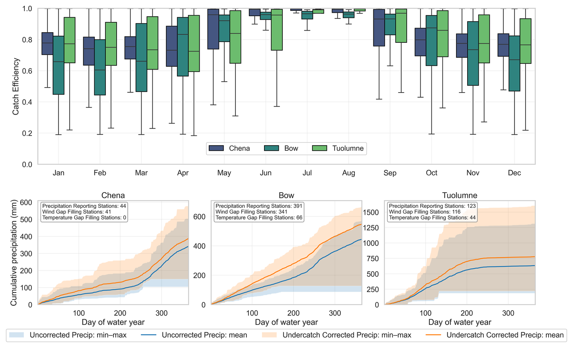
Figure 6 Gauge catch efficiency (CE) and cumulative precipitation across basins. The top panel shows CE correction ranges by month across the Bow, Chena, and Tuolumne basins. The bottom panel shows the effect of undercatch correction on precipitation accumulation over the water year (starting 1 October). Each water year and the mean of all years and stations are shown for each basin. Both the boxplots and area time series summarize calculations at station locations grouped by basin.

The use of reanalysis wind data to enable station undercatch correction was a key step, as shown in Fig. 6. However, reanalysis winds underestimated high wind speeds relative to observations, resulting in conservative catch-efficiency (CE) estimates. This bias was reduced by using daily maximum wind speeds, which better reflect the storm conditions during which snowfall occurs. Even with this adjustment, ERA5-based CE estimates remained conservative, consistent with the tendency of reanalysis products to underestimate site-level wind exposure (Kochendorfer et al., 2017b).

Further detail on the methodological choices and comparisons with reference datasets is provided in Appendix A. Although the approach requires several simplifying assumptions, it effectively captures and corrects wind-induced undercatch, an established and influential source of bias in mountainous snowfall and precipitation measurements.

5.2 Static Predictor Screening with Cross-Validation

The initial screening of static topographic predictors used leave-one-out cross-validation (LWR) and 10-fold cross-validation (RF) at station locations. For each basin, single predictors were evaluated individually, with performance summarized using cross-validated KGE^′′ for daily precipitation (in transformed space) and daily mean temperature. Figure 7 shows the results for the Bow, with analogous figures for the Chena and Tuolumne provided in the Supplement. For single predictors, LWR typically yields slightly higher KGE^′′ than RF, reflecting the advantage of local weighting when only one static covariate is used.

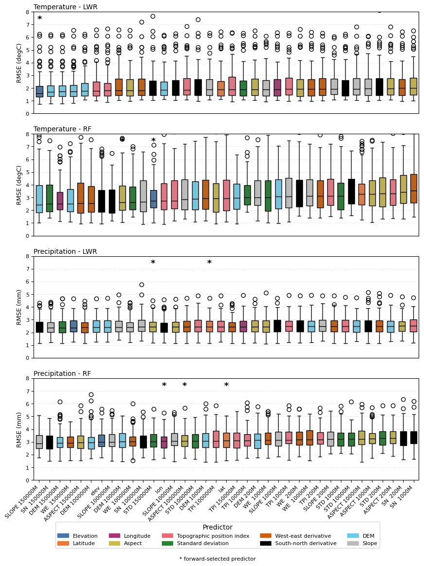
Figure 7 Static predictor screening showing single predictor cross-validation results for the Bow. Topographic descriptors and their smoothed variants (200, 1000, 10 000, 100 000, 150 000 m) are evaluated to assess cross-validation RMSE for temperature and precipitation for both Locally Weighted Regression (LWR) and Random Forest (RF). Asterisk indicates the predictor retained in sequential forward screening.

For temperature, elevation and smoothed DEM fields are consistently skillful predictors for both LWR and RF, reflecting the dominant lapse-rate control on air temperature. Applying spatial smoothing with a larger Gaussian radius (more smoothing) to derived topographic descriptors (e.g., slope, aspect, terrain derivatives) improves cross-validation skill, as smoothing suppresses small-scale noise while retaining large-scale orographic gradients.

For precipitation, the relative performance of individual static predictors is more even. Smoothed variants of terrain descriptors (e.g., South-North and West-East) generally outperform their unsmoothed forms. Across all three basins, predictors smoothed with greater Gaussian radii perform better, indicating that large-scale physiographic structure is more informative than fine-scale terrain details for daily precipitation estimation at the available station density.

Based on the screening results, topographic descriptors smoothed with 100 km Gaussian radius were retained for subsequent predictor combination building, along with unsmoothed elevation, latitude, and longitude.

5.3 Predictor Combination Selection and Regression Performance

Sequential forward screening was used to construct multivariate predictor sets separately for precipitation and temperature, and for each basin and regression method. Starting from an empty model, the static predictor that maximized cross-validated KGE^′′ was selected, after which additional predictors were added one at a time. Predictors were retained only if they increased KGE^′′ by more than 0.01, and the procedure was repeated after allowing dynamic reanalysis-based variables to enter the pool. The resulting optimal combinations are summarized in Table 1.

Table 1 Best static and static + dynamic predictor combinations by catchment, variable, and model (LWR – Locally Weighted Regression, RF – Random Forest).

Across the study basins, elevation or its smoothed derivatives are the primary controls on temperature estimation, with only a small number of additional predictors contributing. For LWR, elevation alone explains most of the variability, while adding a single dynamic predictor (such as reanalysis air temperature or shortwave radiation) provides modest but consistent improvements. RF models for temperature use combinations of elevation and one or two additional topographic descriptors (e.g., aspect or south–north derivative), with further gains when reanalysis air temperature or humidity is included. For precipitation, both static and dynamic predictors contribute. In the Bow basin, LWR identifies aspect and latitude as key predictors, with air temperature as the main dynamic input, while RF additionally includes longitude and surface pressure. In the Chena and Tuolumne basins, RF uses elevation and horizontal derivatives together with reanalysis precipitation rate and surface pressure, indicating that interactions between orography and large-scale meteorology play an important role in daily precipitation patterns within these basins.

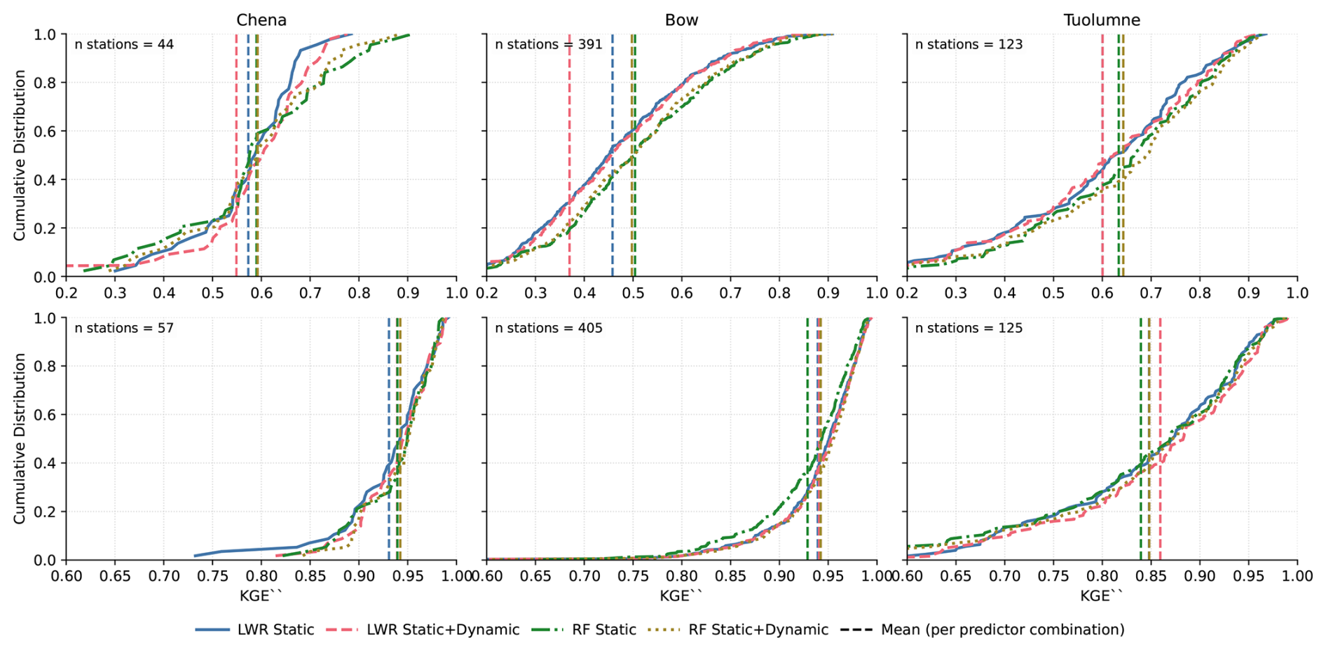
Figure 8 Cross-validation KGE^′′ values for predictor combinations from forward screens. The KGE^′′ for all stations are shown as a cumulative distribution function. Results further to the right of the x-axis are better. The number of stations available for each analysis is shown.

Figure 8 shows the distribution of cross-validated KGE^′′ across all stations for the main predictor combinations. RF systematically outperforms LWR once multiple predictors are available, particularly for precipitation. Adding dynamic predictors further shifts the cumulative distributions to the right, indicating higher skill for the majority of stations. Temperature KGE^′′ is relatively high and similar across methods, whereas precipitation shows a clearer separation between LWR and RF, and between static-only and static + dynamic configurations. It is notable that inclusion of dynamic predictors can degrade the skill of LWR predictions, potentially due to overfitting or creating localized patterns that are not representative.

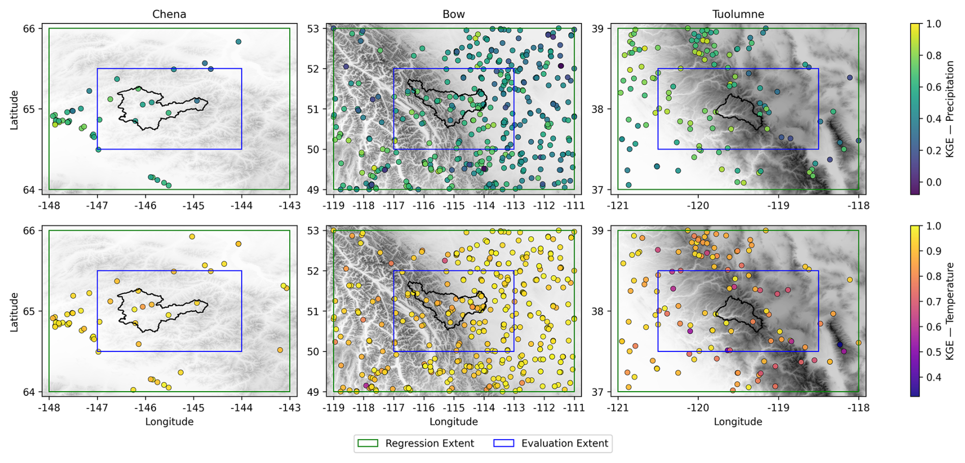
Figure 9 Cross-validation results for Chena, Bow, and Tuolumne River Basins shown as spatial plots for the RF (Random Forest) static and dynamic predictor combinations. Not all stations have both precipitation and temperature measurements. The background map represents elevation.

The spatial pattern of cross-validation performance for the RF static + dynamic combinations is shown in Fig. 9. There is no strong dependence of KGE^′′ on elevation, station density, or location within each basin. Stations achieve ${\mathrm{KGE}}^{\prime \prime }>\mathrm{0}$ for precipitation and ${\mathrm{KGE}}^{\prime \prime }>\mathrm{0.4}$ for temperature, with the proportion of stations exhibiting lower skill not exceeding 3 % for any catchment + variable combination and being 0 % in most cases, likely reflecting localized measurement issues or unresolved sub-grid variability.

5.4 Meteorological Ensembles

Using the selected predictor combinations (Table 1), 50-member daily precipitation and temperature ensembles were generated over each study area. To evaluate the probabilistic skill of these ensembles, we computed Brier Skill Scores (BSS) for station-based events, with climatological occurrence as the reference. For precipitation, the evaluated event was daily precipitation at three thresholds (≥ 0.1, ≥ 5, ≥ 10 mm). For temperature, exceedance events relevant to snow processes were considered (≥ −5 °C,>0 °C, >5 °C).

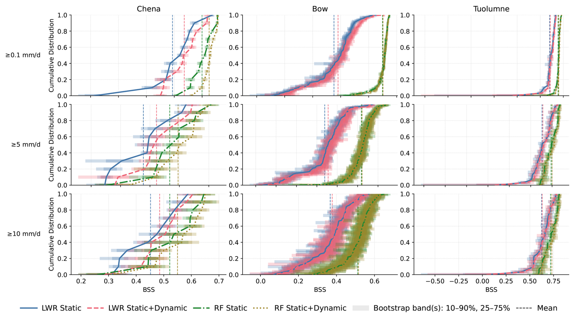
Figure 10 Brier Skill Scores (BSSs) for precipitation with bootstrap resampling. The CDFs of BSSs show the relative performance of each method compared to the climatology mean. BSS=1 indicates a perfect probabilistic prediction, while all values above 0 are better than the climatology.

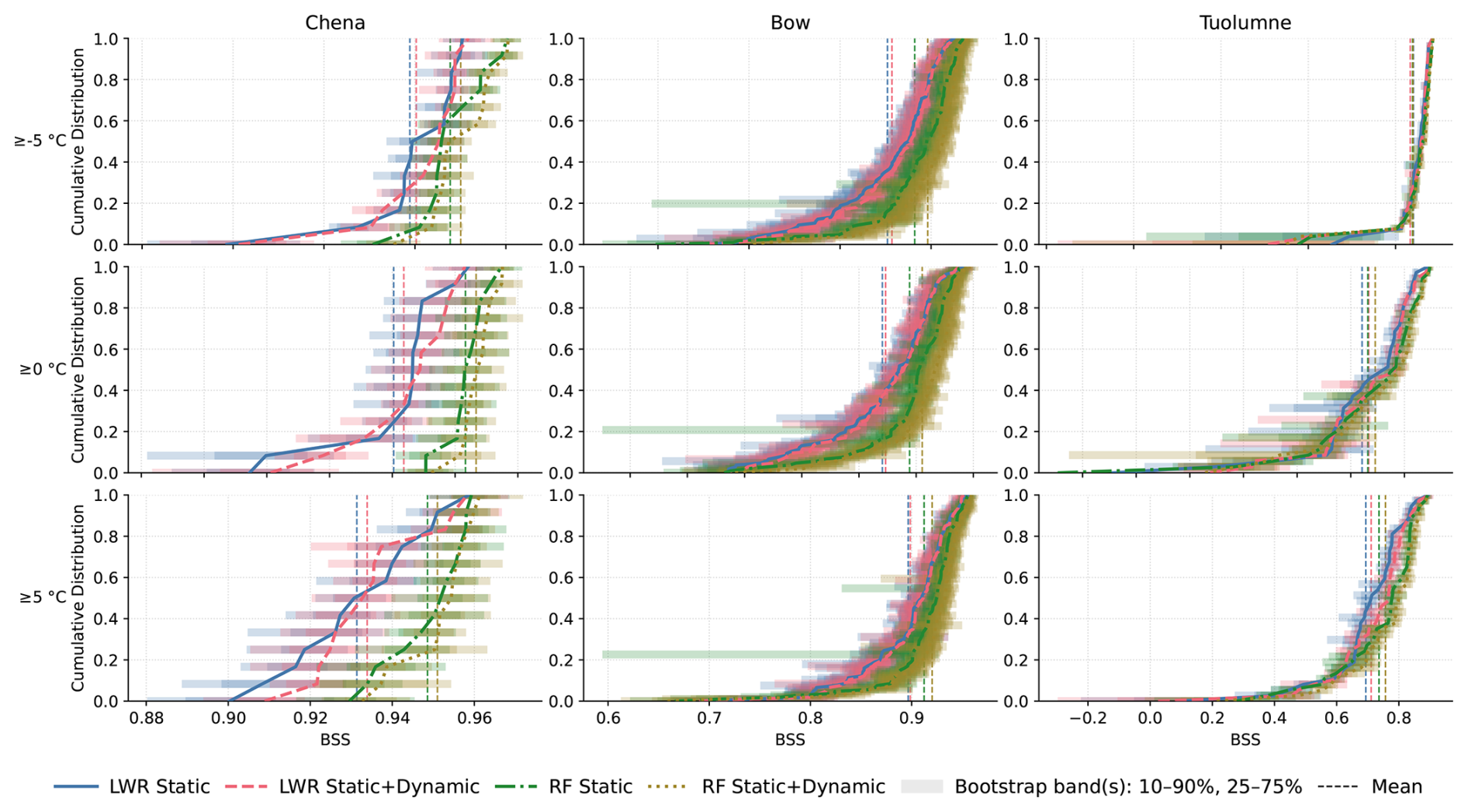
Figure 11 Brier Skill Scores (BSSs) with bootstrap resampling for select temperature thresholds. The CDFs of BSSs show the relative performance of each method compared to the climatology mean. Similar to Fig. 10 but for select temperature thresholds.

Figures 10 and 11 present the cumulative distribution of BSS across all stations for each basin and configuration, along with non-overlapping block bootstrap uncertainty intervals. Positive BSS values indicate that the ensembles provide more information than climatology, with BSS=1 representing a perfect probabilistic forecast. For precipitation, all RF-based ensembles achieve predominantly positive BSS values, with distributions clearly shifted above zero compared to LWR. Incorporating dynamic predictors consistently increases BSS, demonstrating that reanalysis fields add useful information about event occurrence beyond static topography and climatology. LWR ensembles also show positive skill relative to climatology in most basins but with noticeably lower BSS, reflecting limitations of purely local, linear relationships for capturing event-scale variability. Temperature ensembles exhibit higher and more uniform BSS than precipitation across all methods (Fig. 11). RF again outperforms LWR, and static + dynamic configurations yield the highest BSS. The bootstrap uncertainty bands confirm that these differences are statistically robust for the majority of stations. Overall, the ensemble verification indicates that the generated ensembles are skillful and reliable relative to the climatology. RF regression substantially enhances probabilistic performance, particularly for precipitation. The inclusion of dynamic predictors also provides some minor improvements in all cases.

5.5 Snow Modeling

5.5.1 Evaluation with In situ Measurements

The impact of ensemble meteorological forcing on snow simulations was assessed by driving SUMMA with the 50-member RF ensembles and two deterministic benchmark forcings (CaSR and ERA5). Simulations were evaluated for GRUs containing NorSWE manual snow surveys (Fig. 2), with modeled SWE compared against observed transect-based snow surveys. Figure 12 illustrates SWE time series for the three GRUs with the greatest number of snow surveys in each basin.

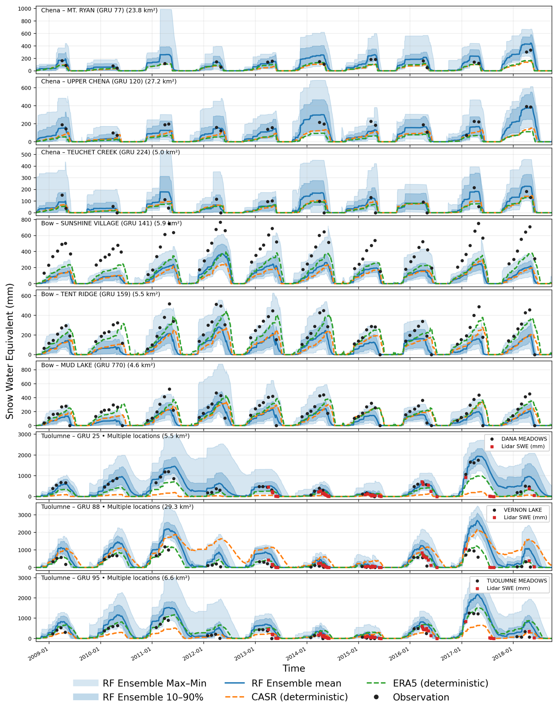
Figure 12 SUMMA sub-basin snow simulations compared to snow surveys. Snow model simulations for the Chena, Bow and Tuolumne are plotted for RF ensembles, CASR, and ERA5 forcing. For each basin the 3 GRUs with the highest amount of snow survey data are shown. For the Tuolumne, lidar SWE estimates averaged over the GRUs are shown.

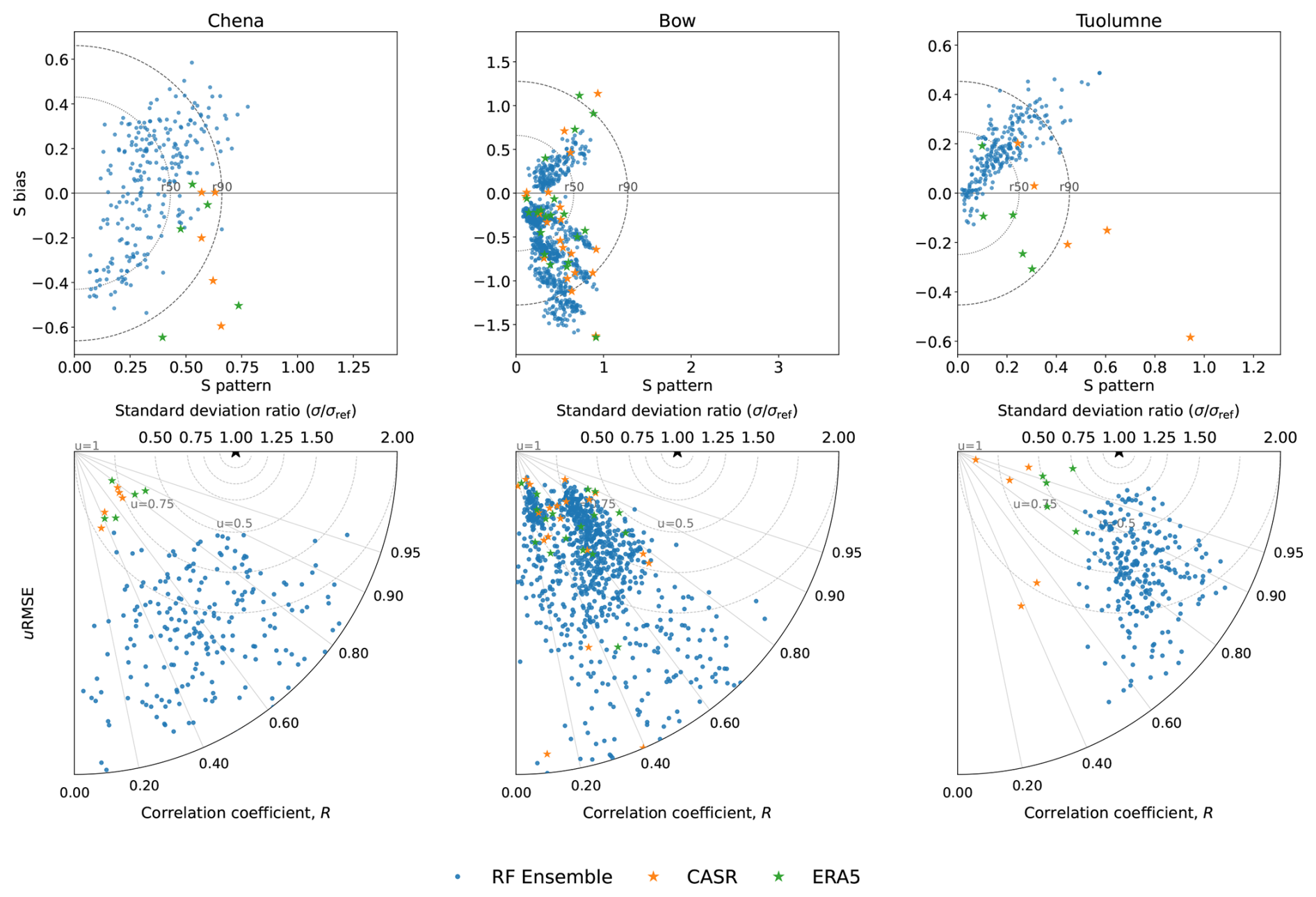
Figure 13 Evaluation of SWE simulations for forcing datasets (Ensemble produced with RF Static–Dynamic predictors (n=50), CaSR, and ERA5) using the skill-target (top row) and Taylor diagram (bottom row). Each point represents a single GRU–forcing pairing (and ensemble member for the RF ensembles). The skill-target diagrams (top) display normalized bias (S bias) versus normalized pattern (S pattern) relative to snow observations; the dashed circles denote 50th and 90th percentiles. Closer to the target origin at zero indicates better performance. The Taylor diagrams (bottom) summarize the same statistics in polar coordinates, with the azimuthal angle representing correlation (R), the radial distance showing normalized standard deviation (S pattern), and contours of equal centered RMSE (u) (Taylor, 2001). Together, the two panels quantify relative skill, bias and correlation consistency following the benchmarking protocol described in Mudryk et al. (2025).

The RF-driven ensembles generally produce larger peak SWE than the deterministic forcings, with observed SWE typically falling within the ensemble spread during the accumulation season. In the Bow, the ensemble mean peak SWE is comparable to the CaSR- and ERA5-driven simulations, whereas in the Chena and Tuolumne the ensembles better capture the range of low- and high-accumulation years, including years when the deterministic forcings substantially under- or overestimate peak SWE. Quantitative evaluation of SWE bias and RMSE (Fig. 13) also illustrates that the RF ensembles provide comparable or improved representation of peak SWE magnitude relative to the deterministic forcings.

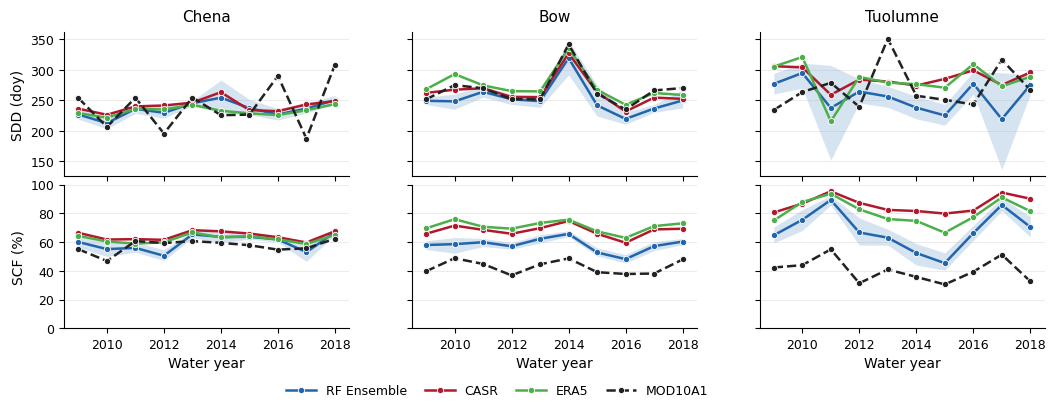
Figure 14 Snow Disappearance Date (SDD) and Snow Cover Fraction (SCF) for snow model results compared to MODIS MOD10A1 derived measurement. Metrics are aggregated spatially over the catchments and calculated for each water year.

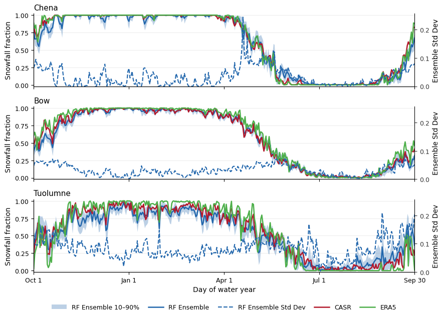
Figure 15 Snowfall fraction (fraction of precipitation that falls as snow) displayed across the water year, including the ensemble spread and standard deviation of ensemble runs.

Agreement at individual survey locations is more variable, and in some Bow GRUs the deterministic simulations more closely match the observed SWE magnitude than the RF ensemble mean. These differences reflect the challenge of evaluating grid-scale simulations using observations that may not fully represent the spatial variability of snow within a GRU. Consequently, the in situ SWE observations primarily constrain snow accumulation and peak SWE, whereas snow disappearance date and snow cover duration are evaluated independently using MODIS-derived products (Fig. 14). Complete SWE time series, including snow pillow evaluations, are provided in Appendix E.

A summary of SWE performance for each basin is provided by the skill-target diagrams and Taylor diagrams in Fig. 13. In the skill-target diagrams, RF ensemble members cluster closer to the origin than ERA5 and CaSR, indicating lower combined pattern and bias error. The RF-based ensemble generally exhibits lower S_pattern values than deterministic forcings, which indicates better modeling of the temporal evolution of snow accumulation and melt. This suggests that ensemble forcing better captures the temperature driven processes and event variability that are often smoothed in reanalysis products. In contrast, differences in S_bias highlight systematic magnitude errors. Deterministic forcings show more consistent but often biased behavior, with pronounced negative SWE bias in the Bow basin, likely linked to precipitation underestimation and unresolved orographic effects. The ensemble spans both positive and negative bias, reflecting uncertainty in precipitation magnitude and phase partitioning. Outlier GRUs with low skill highlight locations where scale mismatch, local wind redistribution, or other unresolved processes strongly influence SWE, regardless of forcing. Taken together, the snow simulation results demonstrate that the station-based meteorological ensembles translate into physically plausible SWE ensembles in SUMMA, the ensemble spread provides a meaningful envelope that contains the majority of observed SWE values; and the RF-based ensemble forcings yield equal or better pattern and bias skill than commonly used deterministic reanalyses, while additionally quantifying uncertainty in snow states.

5.5.2 Evaluation with Remote Sensing Snow Metrics

Snow model results can be compared to the MODIS-derived Snow Cover Fraction (SCF) and Snow Disappearance Date (SDD) (Crumley et al., 2020). The results aggregated spatially per water year are shown in Fig. 14. A spatial comparison of these results is also informative and provided in Appendix D.

Overall, the modeled snow simulations reproduce the magnitude of both snow cover fraction (SCF) and snow disappearance date (SDD) reasonably well compared with the MODIS-derived estimates. Snow cover duration, represented by SCF, is generally overestimated in the Bow and Tuolumne basins, although the RF ensemble exhibits less bias than the ERA5- and CaSR-driven simulations. Interannual variability in SDD is captured more successfully in the Bow than in the Chena and Tuolumne, where year-to-year variations produced by the model correspond less with the derived measurements. It is noted by Stillinger et al. (2023) that MODIS MOD10A1 SCF can have negative bias which may account for part of the lower than modeled values in the Bow and Tuolumne.

5.5.3 Precipitation Phase Uncertainty

Precipitation phase, expressed here as the fraction of precipitation falling as snow, is shown as an annual climatological cycle in Fig. 15. As expected, ensemble uncertainty is greatest during the seasonal transition periods, when precipitation frequently alternates between rain and snow. The Chena exhibits a pronounced peak in ensemble standard deviation during the spring melt period, whereas uncertainty in the Bow is comparatively low. In contrast, the Tuolumne exhibits elevated uncertainty throughout much of the water year, reflecting more persistent uncertainty in precipitation phase. Spatial patterns of precipitation phase, ensemble uncertainty, and normalized uncertainty in water-year snowfall accumulation are presented in Appendix D.

6 Discussion

This study presents an end-to-end approach to representing meteorological forcing uncertainty in physically based mountain snow simulations. The workflow integrates undercatch corrected station-based probabilistic meteorology through to an ensemble forcing and distributed energy-balance snow model simulation. Across three contrasting mountain basins, the approach improves deterministic estimation, yields probabilistic forecasts with positive Brier Skill Scores, and produces snow ensembles that capture the magnitude and timing of SWE with credible uncertainty bounds (Figs. 8, 10, 11, and 13). The contribution lies not only in the individual components but in their coupling: bias corrected inputs and predictor design improve the estimation of meteorology in complex terrain, and these improvements are realized in physically based modeled snow states.

6.1 Ensemble Mountain Meteorology for Snow Modeling

The results advance a long line of efforts to map meteorology in complex terrain and quantify associated uncertainty. Physiographic approaches such as PRISM demonstrated the value of topographic predictors and expert weighting for gridded climatologies (Daly et al., 2008, 2021), while operational products such as seNorge and related systems have emphasized deterministic spatial continuity, but rarely provide event-scale uncertainty (Lussana et al., 2018). Probabilistic geostatistical frameworks, including GMET and subsequent extensions, established that regression against static predictors combined with stochastic sampling of spatially correlated residuals can generate reliable ensembles (Clark and Slater, 2006; Newman et al., 2015). This study builds directly on that foundation by systematically incorporating dynamic predictors from reanalyses alongside static topography and evaluating machine-learning estimators against locally weighted regression within the same ensemble architecture. The finding that RF outperforms LWR for precipitation and temperature in multiple mountain settings strengthens earlier indications that non-linear learners can better represent interactions between orography and time varying patterns (Wolfensberger et al., 2021; Baez-Villanueva et al., 2020).

The Large Sample Emulator (LSE) provides a scalable approach for calibrating physically based snow models across large domains. This builds on recent work by Tang et al. (2025b) and Farahani et al. (2025) in large-domain modeling applications. Rather than relying on basin-specific manual calibration, the emulator transfers information from a diverse set of snow monitoring sites to estimate locally appropriate parameter sets based on climatic and physiographic attributes. This enables spatially varying parameterization while maintaining a consistent calibration methodology across the three study basins. Although the LSE does not reduce structural uncertainty within SUMMA, it provides a reproducible framework for parameter estimation that complements the explicit treatment of meteorological forcing uncertainty presented in this study.

A further contribution is the explicit propagation of this quantified forcing uncertainty into a physically based, energy-balance snow model and its evaluation against in situ SWE observations. Mountain snow modeling studies, whether in multi-model intercomparisons or basin-specific analyses, most often rely on a single deterministic forcing or meteorologic “ensembles of opportunity” constructed from independent reanalyses (Essery et al., 2013; Henn et al., 2018b; Schreiner-McGraw and Ajami, 2022). While useful for assessing dataset spread, such ensembles do not reflect the underlying interpolation and representativeness uncertainties tied to the observing network. In contrast, the ensembles developed here are explicitly conditioned on stations and incorporate spatially structured residual variability, establishing a clearer link between observational density, predictor choice, and modeled uncertainty. The improved representation of SWE magnitude and melt timing relative to ERA5 and CaSR demonstrates the value of carrying realistic input uncertainty through an energy-balance model. The inclusion of MODIS-derived Snow Cover Fraction (SCF) and Snow Disappearance Date (SDD) complements the evaluation based on in situ SWE observations by providing basin-wide assessment of snow persistence and melt timing. While snow surveys constrain SWE magnitude at discrete locations, remotely sensed metrics evaluate the spatial consistency of simulated snow evolution across each watershed. The modeled and MODIS-derived snow metrics generally agree well, though clear biases in SCF vary with topography.

The snow simulation results show that the ensemble framework improves representation of snowpack dynamics while explicitly capturing uncertainty in forcing. Rather than uniformly outperforming deterministic products, the ensemble provides a physically meaningful range of outcomes that reflects sensitivity to precipitation magnitude, phase, and variability. This reveals both improved and degraded simulations across sites, highlighting where deterministic forcings are biased and where snow processes are most sensitive to meteorological uncertainty.

6.2 Methodological Implications

In selecting predictors and estimators for meteorological ensembles, the findings of this study are consistent with process understanding and with lessons from physiographic mapping. Elevation remains the dominant control on temperature, and moderate spatial smoothing of terrain derivatives improves estimation for both variables by emphasizing synoptic structure while retaining key orographic gradients. Dynamic predictors add physically relevant variability that static physiography cannot supply, aligning with the drivers used for land-surface models. The RF advantage over LWR suggests that non-linear interactions among static and dynamic fields are important in sparse mountain networks; at the same time, the LWR framework retains value where transparency and locality are priorities. Because ensemble reliability depends on the fidelity of both the mean and the residual fields, the deterministic gains translate directly into higher Brier Skill Scores once residuals are sampled with spatial correlation.

Workflows such as the one developed for this paper using Snakemake can also contribute to reproducibility and transferability (Köster and Rahmann, 2012). Implementing GPEP with rule-based automation can facilitate consistent application across regions, straightforward selection of predictor sets, and verification. In this study, the use of a standardized discretization (TDX-Hydro) and a consistent SUMMA configuration, coupled with emulator-assisted parameter selection, eased comparative inference across basins. Although such an end-to-end workflow adds an additional software wrapper, as well as dependencies and constraints in conducting such analyses, it also can provide efficiencies in generalizing the analysis.

6.3 Potential Application and Limitations

The study approach provides a practical route for operational agencies and research groups that require uncertainty-aware snow estimates. The approach can harness region specific station measurements and recent gridded analysis to produce skillful ensemble forcing. These data are available in real time, and the procedure can be automated. Driving an energy-balance snow model with these ensembles yields SWE state estimates with credible spread and timing that are directly usable in data assimilation, seasonal outlooks, and risk analyses. The demonstration across three distinct basins suggests that the approach is robust to differences in observing density and topographic complexity, which is essential for scaling to new regions.

Limitations remain across many stages of this approach. Undercatch correction relies on simplifying assumptions on gauge type that should be refined where suitable gauge metadata is available (Huidobro et al., 2023). While reanalysis winds provide a reasonable surrogate for undercatch correction, developing downscaled, gauge-height wind fields for mountains remains a clear priority (Mott et al., 2018; Berg et al., 2024; Marsh et al., 2023; Helbig et al., 2017). The absence of consistent gauge metadata in global archives continues to be a major source of uncertainty for undercatch corrections, reinforcing the need for curated, operator-specific metadata where available (Mekis et al., 2018; Smith et al., 2022; Sun et al., 2019). Daily ensembles subsequently disaggregated into sub-daily forcings limit the representation of diurnal energy fluxes and short-duration events; extending GPEP to hourly resolution could improve melt onset and rain-on-snow timing. The correlation structure and transformation chosen for precipitation influence extremes and dispersion and merit a targeted study. Also, the SUMMA configuration used here does not explicitly represent wind redistribution or avalanching, and GRU-scale evaluation against point or transect observations entails scale mismatch. Furthermore, a single model physics and parameter set is used in this study, so exploration of multi-physics and parameter ensembles could improve probabilistic representation. Finally, further benchmarking with spatial products, such as airborne lidar, could further disentangle and quantify forcing and structural uncertainties.

A key limitation of this framework is the representation of snow processes at the GRU scale, which aggregates substantial sub-grid heterogeneity. Figure 16 illustrates this limitation, showing that SWE measurements collected under contrasting local conditions within a single GRU can differ markedly. Preferential accumulation areas, including wind-sheltered slopes, leeward deposition zones, and forest openings, often sustain deeper and more persistent snowpacks than surrounding terrain, yet are not explicitly resolved. These locations are also underrepresented in meteorological and snow observation networks, compounding uncertainty in both forcing and model evaluation, particularly during melt periods. Although the ensemble framework partially accounts for unresolved variability through spatially correlated perturbations, it does not explicitly represent slope-scale processes such as wind redistribution and preferential deposition. Addressing these limitations will require finer spatial discretization and higher-resolution meteorological forcing, with emerging regional reanalyses and atmospheric models offering improved representation of orographic precipitation and other terrain-driven processes.

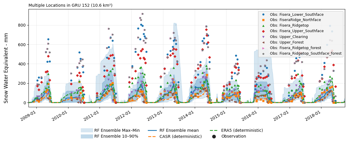
Figure 16 SUMMA SWE simulations of a single GRU with multiple observation sites in the Bow. Measurement location has a large effect on the quantity of snow. This highlights the challenge of evaluation and interpretation of semi-distributed model simulations with in situ data.

In summary, this work extends probabilistic geospatial estimation from the station network to physically based snow modeling and demonstrates that doing so improves both deterministic skill and probabilistic reliability in complex terrain. Relative to the existing literature, it integrates undercatch correction within ensemble construction across multiple catchments, leverages dynamic predictors with a non-linear estimator to enhance station-based ensembles, and shows that the resulting forcings translate into more credible SWE simulations than commonly used deterministic products. The combination of methodological transparency, open implementation, and multi-basin evaluation provides a clear pathway to improve probabilistic snow modeling and water prediction.

7 Conclusions

This study presents a structured approach for propagating meteorological uncertainty through physically based mountain snow modeling. The workflow begins with bias correction of precipitation observations, followed by geospatial estimation of meteorological variables and the generation of high-resolution ensemble meteorological fields. These ensembles capture the spatial and temporal variability of forcing data in complex terrain and are used to drive physically based snow simulations, which propagate input uncertainty into snow estimates. The snow model parameters were calibrated using a Large Sample Emulator. The overall approach was applied and assessed in three contrasting mountain basins: the Chena in Interior Alaska, the Bow in the Canadian Rockies, and the Tuolumne in the Sierra Nevada. These catchments represent a range of climatic conditions, monitoring contexts, and meteorological station densities. Applying this framework within the SUMMA modeling system enabled consistent and transparent representation of meteorological uncertainty in snow state predictions across these diverse settings.

Addressing key deficiencies in mountainous meteorology estimation, namely the influence of complex topography and wind-induced gauge undercatch, improves meteorological estimates. Applying WMO-standard undercatch corrections improves the magnitude of cold-season precipitation estimates. Reanalysis wind data provide a practical supplement where in situ wind measurements are unavailable, enabling consistent correction across large domains. Topographic descriptors, particularly elevation and smoothed terrain derivatives, remain key predictors of both precipitation and temperature patterns. Incorporating dynamic atmospheric predictors from reanalysis further enhances model performance, particularly for precipitation, by capturing synoptic-scale variability that topography alone cannot explain.

Among the deterministic estimation methods, RF-based meteorological estimation consistently outperformed locally weighted regression (the prior default method in studies applying GMET and GPEP), achieving higher cross-validation skill and greater probabilistic reliability once ensemble dressing with spatially correlated errors was applied. Ensemble meteorological forcing fields generated through this framework exhibited markedly higher Brier Skill Scores than climatological references, demonstrating that the ensembles are both reliable and informative. When used to drive physically based snow simulations, these ensembles improved the representation of uncertainty in snow water equivalent, providing a more credible basis for assessing snow-driven hydrologic variability.

Overall, this work highlights the importance and opportunity of explicitly representing meteorological uncertainty in mountain snow modeling. Probabilistic meteorological forcing estimation, when coupled with physically based modeling, provides an effective strategy to bridge the gap between sparse observations and complex terrain processes. The framework nevertheless remains subject to uncertainties arising from precipitation undercatch correction, GRU-scale representation of heterogeneous snow processes, and the use of a single model structure and parameterization, highlighting opportunities for future development. Future developments should aim to extend this ensemble methodology to sub-daily timescales, improve representation of sub-grid mountain processes, incorporate multi-physics and parameter ensembles, and integrate it with data assimilation systems to dynamically constrain snowpack states. As mountain hydrology faces growing challenges from climate variability and changing water demands, probabilistic, physically based approaches such as this offer a foundation for scientific investigation and operational prediction that explicitly includes uncertainty estimates.

Appendix A: Undercatch Correction Methodology

Detailed equations, constants, and assumptions for the undercatch correction methods applied in this study are provided in Table A1. The WMO SPICE UTF (Kochendorfer et al., 2017a, b) is applied in the Bow Basin, while the WMO (1998) standard rain gauge correction (Goodison et al., 1998; Yang et al., 1998) is used for the Chena and Tuolumne basins. Wetting losses are not included in correction. Each approach assumes consistent gauge type and shielding within each basin, reflecting available metadata and historical network standards.

Undercatch correction implementation was compared to the benchmark dataset of Smith et al. (2022) who implemented SPICE UTF methods for stations across Canada. This was performed for overlapping stations (n=10) surrounding the Bow watershed. This comparison highlights differences between shielding assumption configurations, the use of ERA5 winds, and corrections for differences between 2 and 10 m measurement heights. This comparison was performed for the Bow watershed as the assumption of consistent gauge configuration in United States gauging networks is consistent with Newman et al. (2020) and Huidobro et al. (2023). As depicted in Fig. A1, the methodology applied to SC-Earth data matches the seasonality and magnitude of the benchmark dataset. The use of ERA5 winds leads to conservative undercatch compared to in situ data. The selection of shielding configuration is a key assumption, highlighting the need for station metadata across gauging networks.

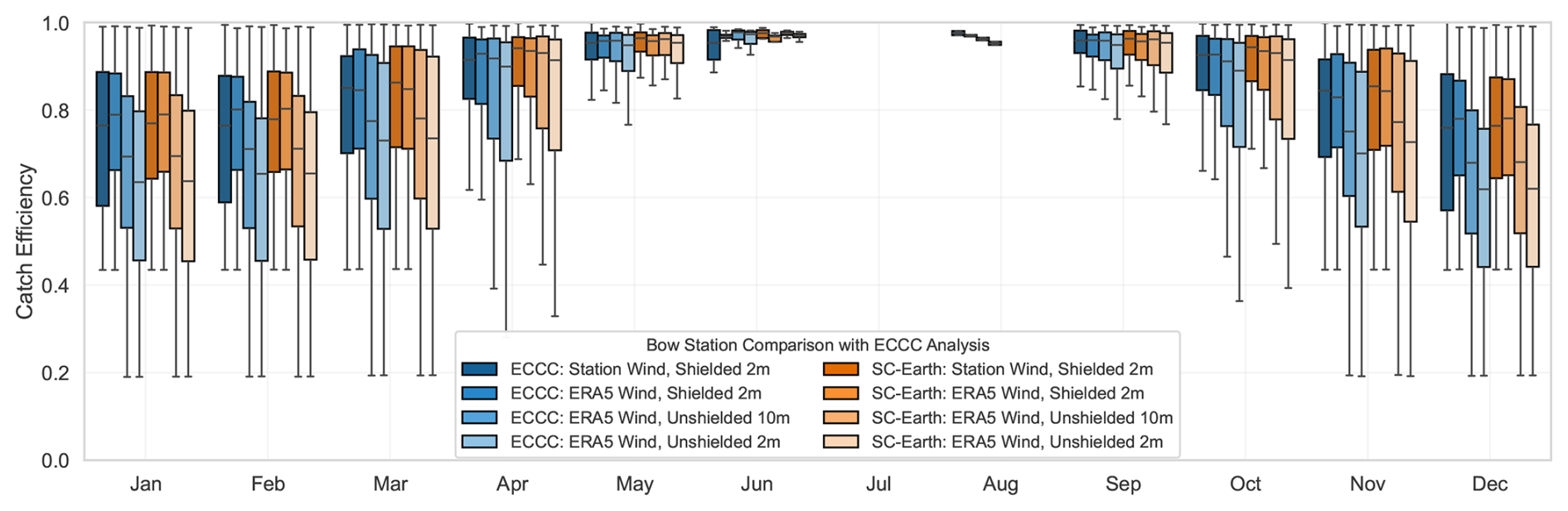
Figure A1 Comparison of methodological choices for undercatch correction using overlapping SC-Earth stations with that of Smith et al. (2022) in the Bow. The shielded 2 m ECCC station dataset represents the reference dataset, while separate iterations assess the effects of supplementing SC-Earth station data with ERA5 winds and applying wind-height corrections.

Kochendorfer et al. (2017a, b)Goodison et al. (1998)Smith et al. (2022)Newman et al. (2020); Froidurot et al. (2014); Huidobro et al. (2023)

Table A1 WMO gauge undercatch methodologies used to correct precipitation measurements in Canadian and US catchments. A simplifying assumption of consistent gauge type within each study area is applied due to limited metadata on gauge configuration.

Appendix B: GPEP Methodology

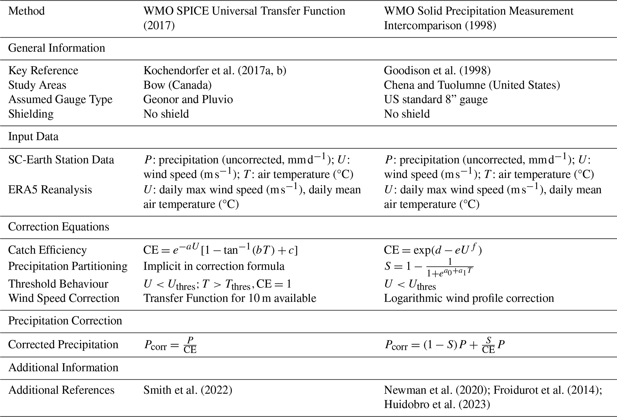
This appendix provides the statistical methods used in the Geospatial Probabilistic Estimation Package (GPEP) for this study. A more complete description of the software and computational considerations is available in Tang et al. (2024). A synthesis of the GMET method development prior to the Python GPEP implementation is also available in Appendix B of Bunn et al. (2022).

B1 Deterministic Estimation

Deterministic estimation forms the first step of the probabilistic workflow. This step estimates the gridded mean of the target variable (e.g., precipitation or temperature measured at station locations) and for intermittent variables the probability of occurrence. These deterministic fields, calculated with locally weighted regression and random forest, form the basis for the ensemble generation process.

B1.1 Locally Weighted Regression

Locally weighted regression (LWR) is used to generate a deterministic grid estimate. For each grid cell, the relationship between the observed or transformed variable x_o and a set of predictor variables A_i is described by

$$\begin{array}{}\text{(B1)}& x_{\mathrm{o}}=\widehat{x}+\mathit{ϵ}={\mathit{\beta }}_{\mathrm{0}}+\sum _{i=\mathrm{1}}^n{A}_i{\mathit{\beta }}_i+\mathit{ϵ},\end{array}$$

where A_i is the ith predictor, β₀ and β_i are regression coefficients, and ϵ is the residual error term. Spatial localization is achieved using distance-based weights that limit the influence of observations to those stations most relevant to the grid cell. This approach allows the regression to capture regional-scale variations while maintaining computational efficiency. As demonstrated by Bunn et al. (2022), the same formulation can incorporate temporally varying predictors such as NWP or reanalysis data.

For variables that are intermittent, such as precipitation, the probability of occurrence is estimated using a locally weighted logistic regression. This calculates the Probability of Precipitation (POP), defined as

$$\begin{array}{}\text{(B2)}& \mathrm{POP}={\displaystyle \frac{\mathrm{1}}{\mathrm{1}+\exp \left(-\left({\mathit{\beta }}_{\mathrm{0}}+{\sum }_{i=\mathrm{1}}^n{A}_i{\mathit{\beta }}_i\right)\right)}}.\end{array}$$

The resulting mean field and probability field are then used in the probabilistic estimation step to generate ensemble realizations that reflect both the expected value and its associated uncertainty.

B1.2 Random Forest Regression and Classification

Random forest (RF) methods provide a non-parametric alternative to locally weighted regression for generating the deterministic estimate. RF models can be applied in both regression and classification modes, corresponding, respectively to the estimation of continuous variables (e.g., precipitation amount, temperature) and the prediction of event probabilities (e.g., precipitation occurrence) (Wolfensberger et al., 2021). Within the geospatial probabilistic estimation framework, RF regression and classification serve analogous roles to the locally weighted linear and logistic regression, respectively.

An RF model consists of an ensemble of decision trees, each trained on a random subset of the available data and predictor variables (Breiman, 2001). This process introduces stochasticity in both the sampling of training observations (via bootstrapping) and the selection of predictors at each node, ensuring that the ensemble captures a diverse range of predictor–response relationships. The final prediction is obtained by aggregating the outputs of all trees, which improves generalization and reduces overfitting relative to a single decision tree (Cutler et al., 2007).

In regression applications, each tree produces an individual prediction ${\widehat{x}}_j$ of the variable of interest x_o, based on a set of predictors $A_{\mathrm{1}},A_{\mathrm{2}},\mathrm{\dots },A_n$. The ensemble mean prediction $\widehat{x}$ is then computed as the arithmetic average across all T trees:

$$\begin{array}{}\text{(B3)}& \widehat{x}={\displaystyle \frac{\mathrm{1}}{T}}\sum _{j=\mathrm{1}}^T{\widehat{x}}_j,\end{array}$$

where T is the number of trees in the forest and ${\widehat{x}}_j$ is the prediction from the jth tree. Each decision tree recursively partitions the predictor space by selecting split thresholds that minimize a specified cost function. The averaging of multiple decorrelated trees yields a stable estimate that reflects nonlinear relationships between predictors and responses without requiring an explicit parametric model (Tyralis et al., 2019).

In classification applications, each tree predicts a categorical outcome ${\widehat{y}}_j$, such as the presence or absence of precipitation. The ensemble classification $\widehat{y}$ is determined by majority voting across the T trees:

$$\begin{array}{}\text{(B4)}& \widehat{y}=\mathrm{mode}({\widehat{y}}_{\mathrm{1}},{\widehat{y}}_{\mathrm{2}},\mathrm{\dots },{\widehat{y}}_T),\end{array}$$

where mode(⋅) denotes the most frequent class among the tree-level predictions. The result is a probability of occurrence derived from the fraction of trees that predict a given outcome, which can be used as the Probability of Precipitation (POP) in probabilistic estimation.

The RF models in GPEP are implemented using the scikit-learn library, enabling straightforward implementation (Pedregosa et al., 2011). Unlike locally weighted regression, RF models are inherently global: they are trained once using all available stations and predictor data, rather than fitting a separate model at each grid cell. This global structure allows the RF approach to exploit complex, nonlinear dependencies between predictors (e.g., topography, dynamic atmospheric predictors, and spatial coordinates), while maintaining computational scalability across large domains (Fox et al., 2020).

Random forests, therefore, provide a robust and flexible alternative for deterministic gridded estimation of geospatial variables, particularly in regions where predictor–response relationships are highly nonlinear or where the spatial sampling of observations is sparse or irregular (Sekulić et al., 2020). The mean field and probability field outputs from RF regression and classification are subsequently used in the probabilistic estimation step, where uncertainty is represented through spatially correlated ensemble generation.

B2 Probabilistic Estimation and Ensemble Generation

The probabilistic estimation stage converts the deterministic fields into ensemble realizations that represent the spatial and temporal uncertainty of the estimated variables. This is achieved by combining the deterministic mean estimates, the associated uncertainty calculated from station error, and a stochastic component represented by spatially correlated random fields (SCRFs). The SCRFs ensure that the generated ensembles preserve realistic spatial coherence and correlation structures that are consistent with those observed in the station data and predictor fields.

In the general case, a variable X at a given grid cell and time step is represented as a random variable drawn from a Gaussian probability distribution, written in-text as $X\sim \mathcal{N}(\mathit{\mu },{\mathit{\sigma }}^{\mathrm{2}})$, where μ corresponds to the deterministic mean estimate and σ quantifies local uncertainty. For variables such as temperature and temperature range, this normal approximation is appropriate. For intermittent and skewed variables such as precipitation, the distribution is decomposed into two components: the probability of occurrence (p₀) and the conditional distribution of nonzero values. The conditional precipitation field is transformed to normal space using a Box–Cox or power-law transformation to ensure approximate Gaussianity (Newman et al., 2015; Tang et al., 2024).

To represent spatial structure, ensemble perturbations are generated using SCRFs sampled from a standard normal distribution. The SCRFs impose correlation among neighboring grid cells using an exponential correlation model:

$$\begin{array}{}\text{(B5)}& c_{i,j}=\exp \left(-{\displaystyle \frac{d_{i,j}}{L_{\mathrm{c}}}}\right),\end{array}$$

where c_i,j is the correlation between grid cells i and j, d_i,j is the distance between them, and L_c is the spatial correlation length. The correlation length is estimated empirically from station data and varies by variable and domain. SCRFs are generated using a conditional simulation approach (Clark and Slater, 2006), ensuring that each random field realization maintains both the specified correlation structure and the correct marginal statistics.

Temporal coherence is introduced by linking random fields across successive time steps using lag-1 autocorrelation coefficients derived from the observed data. Cross-variable correlations (for example, between precipitation and temperature range) can also be imposed to maintain realistic multivariate relationships (Tang et al., 2024).

For each ensemble member, the SCRFs are used to perturb the deterministic estimates according to their local uncertainty. For normally distributed variables such as temperature, the probabilistic estimate is computed as

$$\begin{array}{}\text{(B6)}& x=\mathit{\mu }+R\cdot \mathit{\sigma },\end{array}$$

where R is the corresponding value from the SCRF in that grid cell and time. For intermittent variables such as precipitation, ensemble generation proceeds in two steps. First, the probability of occurrence is evaluated: if the cumulative probability of R is less than the occurrence probability p₀, the grid cell is assigned zero precipitation. Otherwise, the nonzero precipitation amount is computed by scaling and back-transforming the random draw in normal space:

$$\begin{array}{}\text{(B7)}& y=\left\{\begin{array}{ll}\mathrm{0},& \mathrm{if}{F}_N\left(R\right)\le p_{\mathrm{0}},\\ \mathit{\mu }+F_N^{-\mathrm{1}}\left(\frac{F_N\left(R\right)-p_{\mathrm{0}}}{\mathrm{1}-p_{\mathrm{0}}}\right)\mathit{\sigma },& \mathrm{if}{F}_N\left(R\right)>p_{\mathrm{0}},\end{array}\right.\end{array}$$

where F_N(⋅) and $F_N^{-\mathrm{1}}(\cdot )$ are the standard normal cumulative distribution and its inverse. The resulting y values are then inverse-transformed from normal space to yield precipitation in physical units. This process is repeated independently for each ensemble member, generating a suite of spatially and temporally coherent realizations.

Appendix C: Large Sample Emulator Errors Compared to SUMMA

For the 162 stations used to train the emulator (in red in Fig. C1), we compared the Taylor Skill Score (TSS; Taylor, 2001) from SUMMA (i.e., simulations vs. observations) and the emulated TSS value using random forest (Fig. C1b). The emulator comprises 162 000 SUMMA simulations (162 stations × 1000 parameter sets; density dots in Fig. C1b), for step i=5 of the iterative process. To obtain new parameter sets for each station, we search the emulated response surface using a Genetic Algorithm (GA), yielding 100 new parameter sets per station. SUMMA is then run for these parameter sets to compute TSS, providing an evaluation error for parameter sets unseen during random forest training. At step i=5, the MAE between emulated and SUMMA TSS values for these unseen parameter sets is 0.242 TSS units. We also apply the trained emulator from each iteration step to search for parameter sets at unseen stations (shown in red in Fig. C1c, n=608), again using a GA to produce 100 candidate parameter sets per station. The error between emulated and SUMMA TSS values is then computed across these 608 stations × 100 parameter sets. As shown in Fig. C1d, this error decreases steadily across iteration steps, reflecting both the growing training dataset – which increases from 500 to 1000 parameter sets per station between i=0 and i=5 – and the progressively better-explored parameter space.

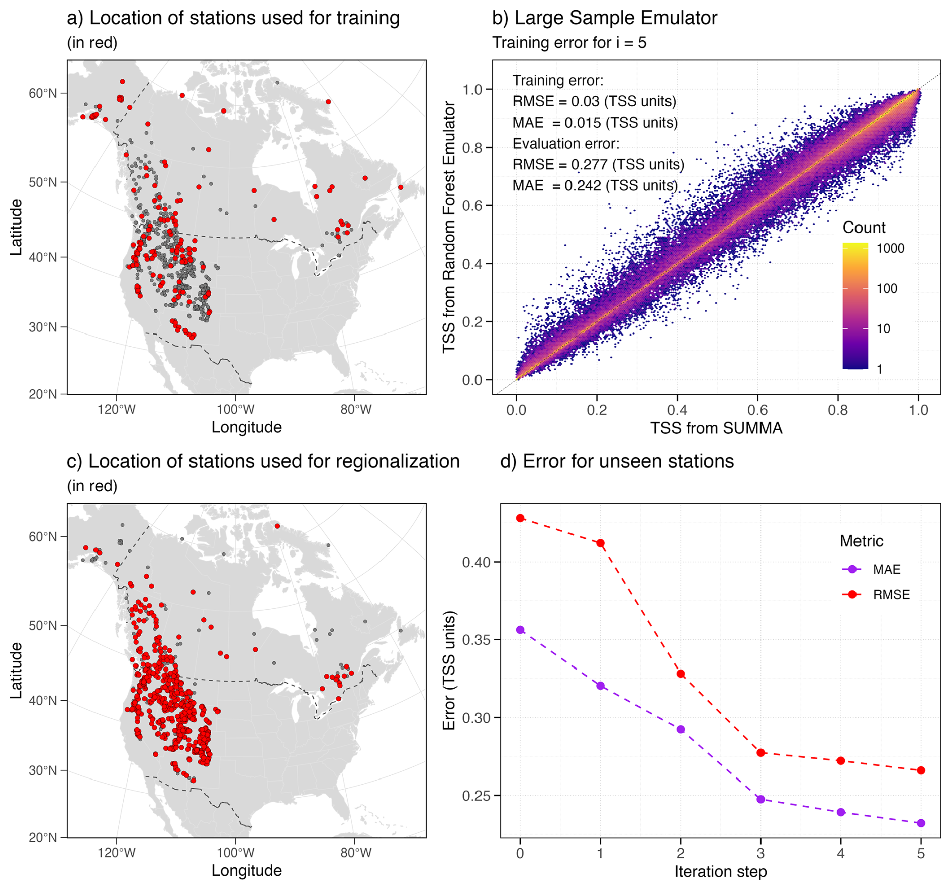
Figure C1 Emulator errors for training and unseen stations. (a) Location of the basins (in red) used to train the emulator (n=162). (b) Training error for emulator at iteration step i=5, and evaluation errors for the new parameter sets obtained through the Genetic Algorithm optimization search. (c) Stations used for parameter regionalization (i.e., unseen stations, n=608). (d) Root Mean Square Error (RMSE) and Mean Absolute Error (MAE) between SUMMA TSS and emulated TSS for the unseen stations and from the emulator trained for each step of the iterative process to refine the emulator.

Appendix D: Spatially Distributed Snow Measurement and Precipitation Phase Results

Spatially distributed results are provided in this appendix to illustrate how spatial patterns and biases are present. This is presented first for the comparison of model results to MODIS derived snow metrics in Figs. D1 and D2 followed by assessment of precipitation phase uncertainty in Fig. D3.

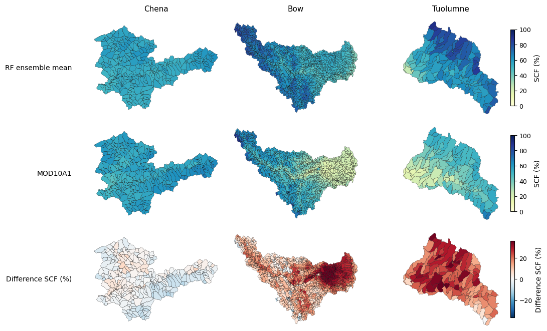
Figure D1 Snow Cover Fraction (SCF) averaged over all water years (2010–2018). This plot shows the RF ensemble mean result, the MODIS measurement, and the difference between them. Snow Cover Fraction (SCF) is overestimated in lower elevation sub-basins in both the Bow and the Tuolumne. This would contribute to an overestimation in catchment mean. Chena results are more consistent spatially and show closer agreement between model and measurements.

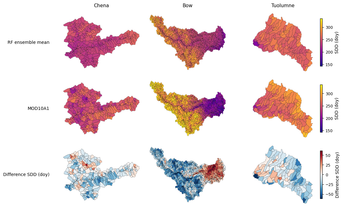
Figure D2 Snow Disappearance Date (SDD) averaged over all water years (2010–2018). This plot shows the RF ensemble mean result, the MODIS measurement and difference between. Comparable to the SCF result, the SDD is overestimated in the lower elevations for Bow and Tuolumne while the upper elevation sub-basin SDD tends to be more underestimated by the model.

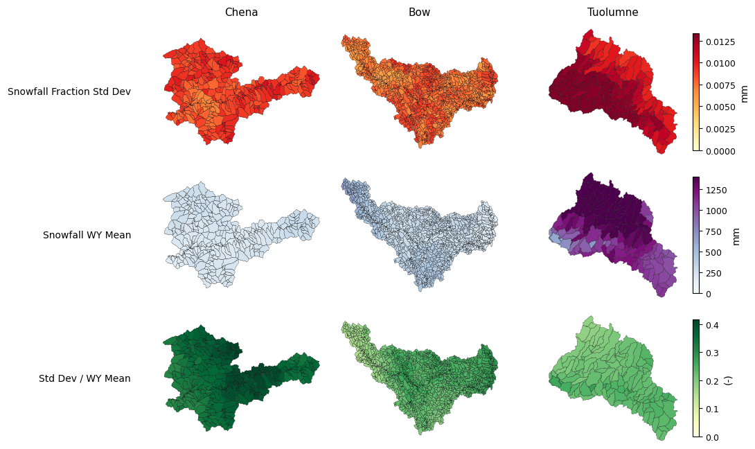
Figure D3 Snowfall fraction is calculated across ensemble members and the standard deviation used to represent precipitation phase uncertainty. The uncertainty in precipitation phase across the simulation period does not indicate a distinct spatial pattern, with the exception of high uncertainty at Tuolumne lower elevations. Normalizing the standard deviation by the total mean water-year snowfall allows comparison across basins.

Appendix E: Complete SWE Timeseries Results

The complete SWE timeseries allowing comparison between modeled and measured results is shown in Fig. , and E3.

Figure E1 Chena SUMMA Snow Simulation Timeseries compared to NorSWE observations.

Figure E2 Bow SUMMA Snow Simulation Timeseries compared to NorSWE observations.

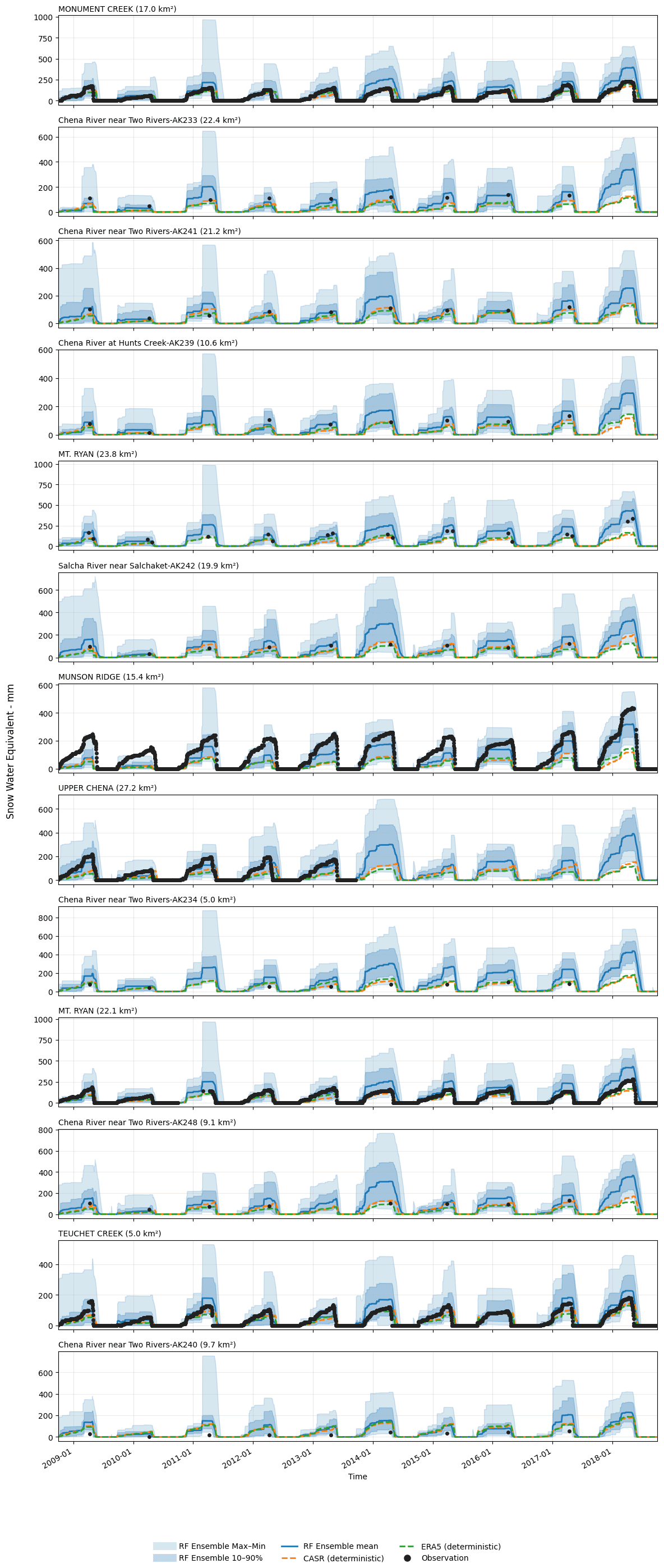
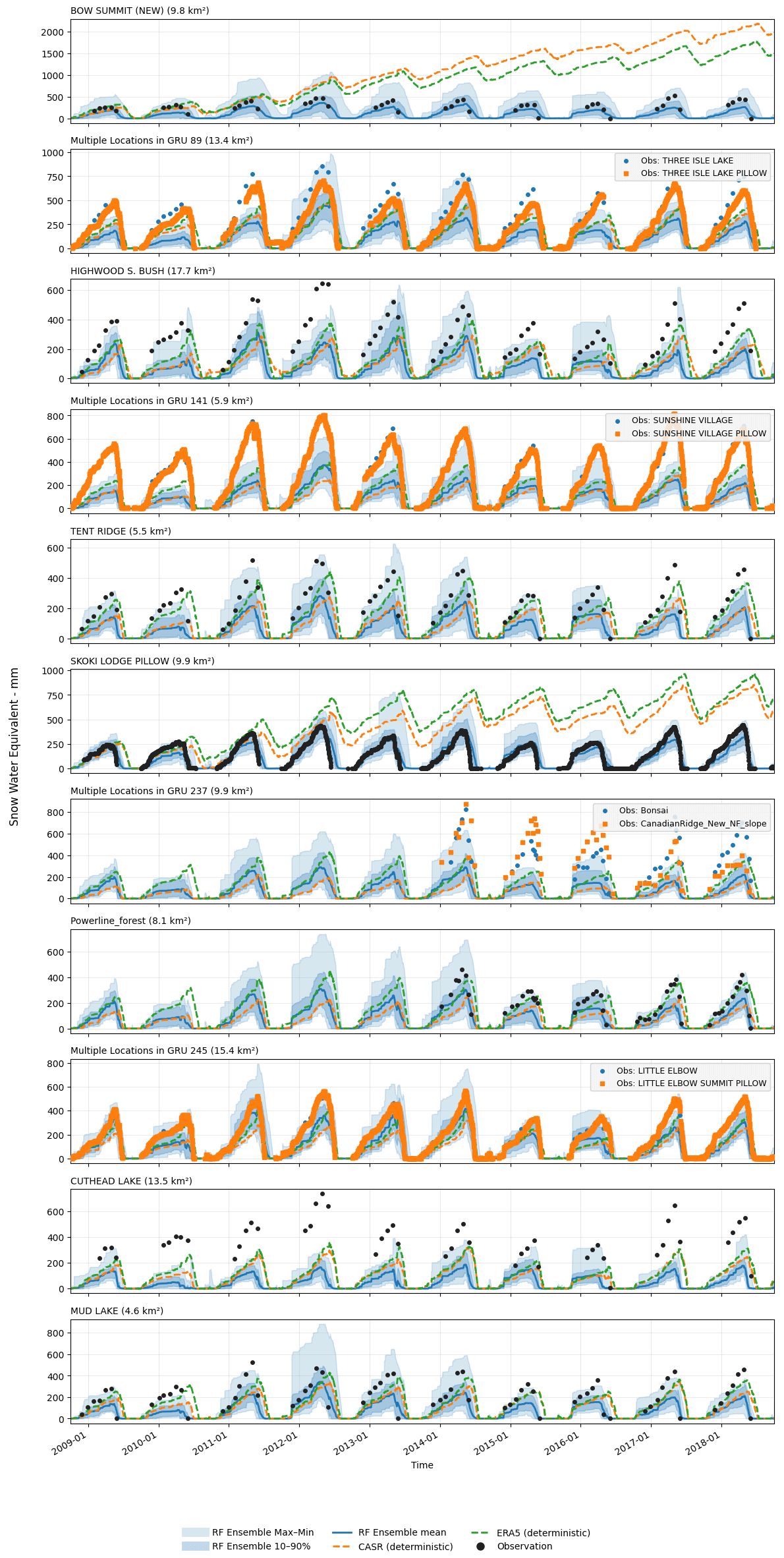
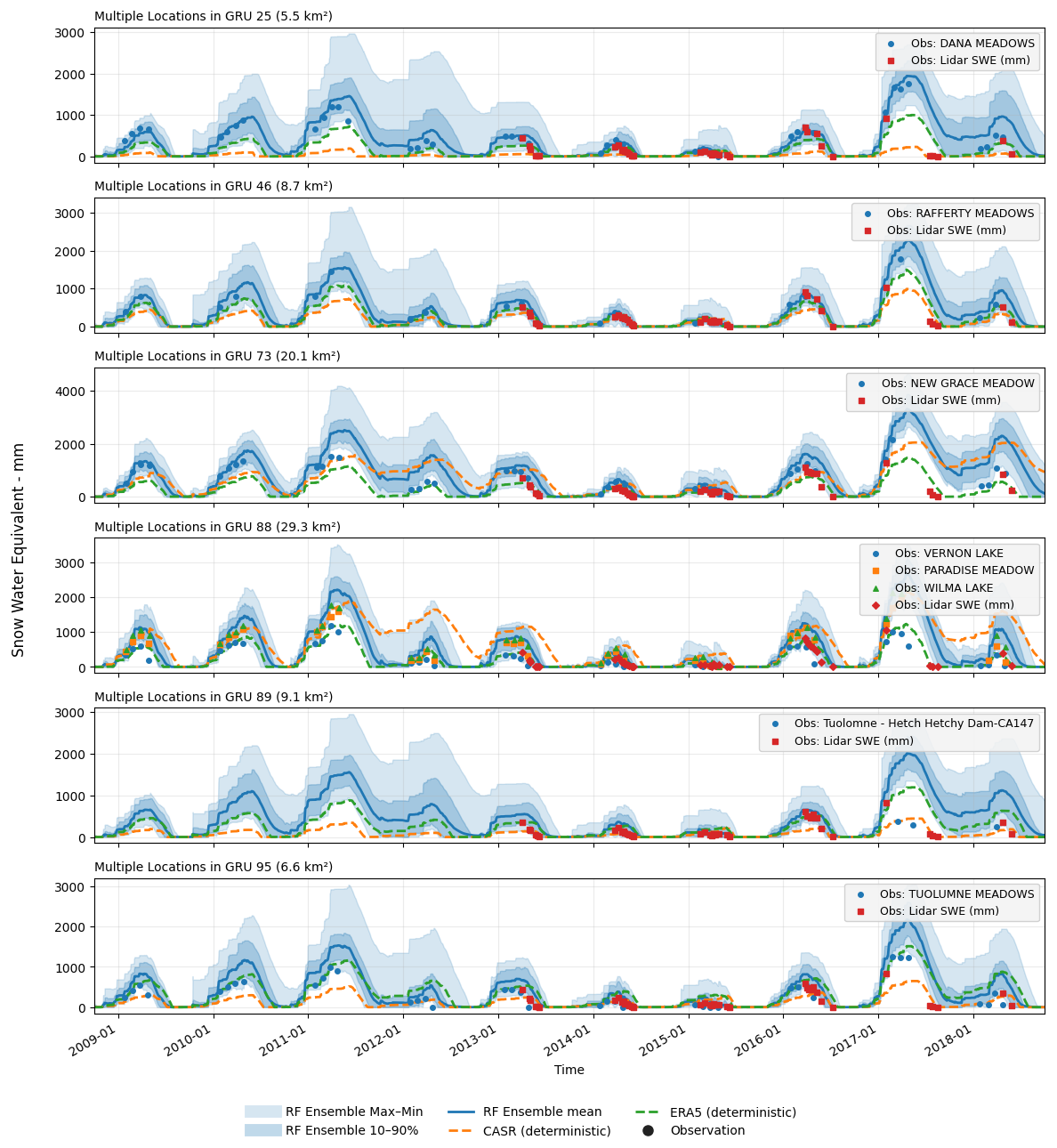
Figure E3 Tuolumne SUMMA Snow Simulation Timeseries compared to NorSWE observations. ASO lidar estimates of SWE are also shown as sub-basin averages from 2014–2018.