Modelling climate-induced instability of ice-rich permafrost slopes

Climate-induced slope failures in ice-rich permafrost environments typically manifest in surficial materials as active layer detachment failures (ALDF) and as newly initiated retrogressive thaw slumps (RTS). Instability is linked to high pore water pressures developed during thaw of ice-rich layers that reduce the factor of safety below unity. Here we develop a module within the CryoGrid community model that uses meteorological inputs and soil geotechnical characteristics to simulate ice segregation and thaw consolidation, and predicts potential instability at all levels within the soil column through time using an infinite slope analysis. The analysis is expanded spatially using clustering of slope gradients and aspect. The model was tested using a multi-decadal database of RTS initiation for an area of 2300 km² on Banks Island, Canada. We used RTS as a proxy for ALDF, since the majority of RTS in the field area were triggered in warm summers by exposure of massive ice following ALDF. Results showed that the Thawing Slope Stability Index (TSSI), based on the severity and duration of slope instability, was correlated with years in which tens to hundreds of RTS were initiated. These years were characterized by high summer air temperatures and high incoming short-wave radiation which led to a deepening of the active layer in the model, melting of ice-rich layers, and increased pore water pressures. Furthermore, the newly initiated RTS were concentrated on slopes with the highest TSSI values. The newly developed modelling scheme represents a significant step towards evaluating the stability of ice-rich permafrost slopes for different land use and climate change scenarios.

1 Introduction

Permafrost environments are experiencing major changes due to rising ground temperatures and increasing active layer thicknesses (Biskaborn et al., 2019). Widespread warming and degradation especially impact ice-rich permafrost landscapes where melting of excess ice and thermokarst development have significant consequences (Kokelj and Jorgenson, 2013; Olefeldt et al., 2016) on hillslope processes (Segal et al., 2016; Swanson, 2021), ground subsidence (Liu et al., 2015; Farquharson et al., 2019), and lake formation and drainage (Jones et al., 2011; Chen et al., 2023). Furthermore, thaw can contribute to the mobilization of permafrost carbon, establishing a positive feedback loop that further increases atmospheric carbon concentrations (Miner et al., 2022).

In sloping terrain, thawing of ice-rich permafrost can result in two main types of slope failure: active-layer detachment failures (ALDF) (Jorgenson and Osterkamp, 2005; Lewkowicz and Harris, 2005; Lewkowicz, 2007; Lamoureux and Lafrenière, 2009), and retrogressive thaw slumps (RTS) (Nesterova et al., 2024). ALDF are shallow translational landslides ranging in length from a few metres to a few hundred metres in which unfrozen soils move downslope over a thaw plane or a thin shear zone within the transient layer near the base of the active layer or in the uppermost permafrost horizons (Lewkowicz et al., 2025). ALDF typically remain active for a few hours to a few days and then stabilize (Lewkowicz, 2007). In contrast, RTS extend deeper into the permafrost and feature ice-rich headwalls that range from less than 1 m to tens of meters in height. After initiation, RTS enlarge progressively during the thaw season as ablation of the exposed ground ice or icy sediments undercuts the overlying active layer or ice-poor material and the resultant material and water are evacuated downslope (Nesterova et al., 2024). RTS stabilize each autumn when the ground refreezes but can re-activate in the spring and may expand for decades, potentially becoming megaslumps (Kizyakov et al., 2023).

Despite the differences in the morphology, process and evolution of ALDF and RTS, thaw consolidation is the critical process underlying both ALDF formation (Morgenstern and Nixon, 1971; McRoberts and Morgenstern, 1974) and RTS initiation. Thaw consolidation is the “time-dependent compression resulting from thawing of frozen ground and subsequent expulsion of excess water” (Lewkowicz et al., 2025). If thaw is rapid enough in fine-grained soils, some liberated meltwater may be unable to drain and high pore water pressures can develop. The latter reduce the soil's effective strength, causing the factor of safety (shear strength divided by shear stress) to fall below unity, resulting in unstable conditions and potential slope failure (Salunkhe et al., 2017).

The development of high pore water pressures during thaw has long been known to be linked to the formation of ALDF (e.g.,  McRoberts and Morgenstern, 1974). They develop in Arctic, sub-arctic and mountainous settings and occur over a wide range of slope angles (Niu et al., 2016; Bernhard et al., 2021; Leibman et al., 2023) and aspects (Bernhard et al., 2021; Nesterova et al., 2021). Initiation of ALDF in ice-rich permafrost is often associated with years of extreme weather conditions, such as warm summers (Lewkowicz, 2007; Lamoureux and Lafrenière, 2009; Lacelle et al., 2010; Balser et al., 2014) or intense precipitation and snow melt (Lamoureux and Lafrenière, 2009; Balser et al., 2014). Such conditions result in higher ground temperatures, a deepening of the active layer and thawing of the uppermost layers of ice-rich permafrost.

The initial exposure of ice-rich permafrost needed for RTS initiation (as opposed to the processes that cause RTS enlargement) was generally assumed to relate to slope under-cutting and blockfall caused by localised erosion at coasts, along lakeshores or adjacent to rivers (Burn and Lewkowicz, 1990). RTS were also known to initiate in the scar zones of ALDF (Lacelle et al., 2010; Lewkowicz and Way, 2019). Recent studies showing that hundreds of RTS can be initiated in differing positions within the landscape in the same thaw season (Lewkowicz and Way, 2019; Lewkowicz, 2024), however, demonstrate that slope instabilities leading to RTS initiation must be far more widespread than can be explained by localized fluvial, lakeshore or coastal erosion.

Several studies have presented methods to calculate the factor of safety in permafrost slopes based on the pore water pressure. Most assume a planar failure on an infinite slope (Chandler, 1972; Hutchinson, 1974; McRoberts and Morgenstern, 1974; Lewkowicz and Harris, 2005; Niu et al., 2016; Fiolleau et al., 2024), which is appropriate for a rigid mass that fails over a thin shear zone (Lewkowicz and Harris, 2005), such as for ALDF (Lipovsky et al., 2005). These studies performed sensitivity analyses by varying the parameters to calculate the factor of safety. Others included ground temperature variations to evaluate changes in the slope stability (Zhang et al., 2022).

Previous studies have developed maps showing the susceptibility of terrain to RTS initiation (Li et al., 2024). These maps were based on a set of influencing factors, including topography, permafrost and soil characteristics, atmospheric data, and hydrology, which were weighted according to their importance (Niu et al., 2014; Blais-Stevens et al., 2015). To avoid subjective factor weights, statistical models and machine learning approaches were introduced to improve model performance (Liu et al., 2021; Yin et al., 2021; Makopoulou et al., 2024, 2025). However, it is clear that a physically-based model would be better suited for evaluating the effects of climatic variation or change which are known to strongly influence slope stability in permafrost environments (Nesterova et al., 2024).

In this study, we calculate the factor of safety within the framework of a land surface model and evaluate the potential for slope failure by introducing the Thawing Slope Stability Index (TSSI). This approach represents a physically-based, climate-dependent assessment of the susceptibility to ALDF in ice-rich permafrost. We demonstrate the new model functionalities with multi-decadal simulations for a study area on Banks Island, Canada, and compare our results with a long-term inventory of newly initiated RTS (Lewkowicz and Way, 2019).

2 Methods

We used the CryoGrid community model (Westermann et al., 2023), in particular the CryoGrid geomechanical scheme (Aga et al., 2023), to calculate the factor of safety in sloping permafrost terrain through time and space. The modular framework of the CryoGrid community model is designed to simulate the ground thermal regime in permafrost areas, including the water/ice balance in the ground. Users can select from various stratigraphy classes, each characterized by distinct model physics and state variables, such as a different realization of the water fluxes or the freezing characteristics of the soil. Additionally, specific stratigraphy classes handle non-ground materials, such as the seasonal snow cover. The stratigraphy classes can be stacked vertically, thereby providing the flexibility to combine snow-related classes with differing ground material classes.

The CryoGrid geomechanical scheme simulates water fluxes in saturated and unsaturated soils, calculates pore water pressures, and models ice segregation and thaw consolidation (Aga et al., 2023). Based on these results, the factor of safety can be computed over time at multiple levels within the soil column.

2.1 Model description

A comprehensive summary of the CryoGrid community model is given in Westermann et al. (2023) and a detailed description of CryoGrid geomechanical scheme is provided in Aga et al. (2023). Here, we present an overview of relevant information and equations (Sect. 2.1, Fig. 1), describe the study area (Sect. 2.2), and present the forcing data (Sect. 2.3) and parameters (Sect. 2.4) for the model scenarios.

2.1.1 Existing model functionalities

Stratigraphy classes in the CryoGrid community model describe the subsurface and are defined by grid cells consisting of mineral and/or organic matter together with a water and an ice phase. These components are quantified in terms of individual volumetric content which also determines the porosity of the system. The upper boundary of this class represents the interface between the ground surface and the atmosphere. The surface energy balance computed at this boundary comprises short-wave and long-wave radiation, latent and sensible heat fluxes. This requires model inputs of a time series of air temperature, solid and liquid precipitation, wind speed, short-wave and long-wave radiation, specific humidity and air pressure. The lower boundary is characterized by a constant geothermal heat flux set at a depth specified by the user. The CryoGrid community model computes both conductive and convective heat fluxes within the ground. The former is based on Fourier's law, where the dominant factor is the thermal conductivity of the ground. The latter is governed by water fluxes in the soil, driven through gravity in the saturated domain and gradients of the matric and gravitational potential in unsaturated conditions.

The CryoGrid geomechanical scheme computes the stress conditions in the soil, with the total normal stress being the sum of the vertical geostatic stress and external loads. The normal stress varies over time with changes in the weight of the overlying soil. As the mineral and organic content stays constant throughout the simulation, variations are controlled by the water balance, namely infiltration and evaporation, while variations in density due to phase changes of the water were not considered to ensure compatibility with other CryoGrid modules. The effective stress acting on the soil matrix is subsequently obtained by subtracting the pore water pressure from the normal stress, i.e. reducing the density of the soil by the density of water in saturated conditions (Aga et al., 2023). As the effective stress increases (decreases), the soil undergoes compression (relaxation). This process induces changes in the porosity that depend on a soil-specific compression curve, allowing ground heave and subsidence to be computed (Aga et al., 2023).

The stratigraphy class also incorporates a water retention curve which determines the soil freezing characteristics, i.e. the relationship between ground temperature and unfrozen water content (Painter and Karra, 2014). To evaluate the liquid water and ice content, the matric potential is computed for unfrozen states using the van Genuchten model (Van Genuchten, 1980). Subsequently, the matric potential for frozen conditions is derived, which in turn enables the determination of the liquid water content within the frozen soil. Westermann et al. (2023) provides a detailed description of this approach.

Under saturated conditions, water flow resulting from gravity follows the principles of Darcy's law. If the ground is unfrozen and unsaturated, the vertical water flux $j_{\mathrm{w}}^{\mathrm{v}}$ [m s⁻¹] is controlled by Richard's equation (Richards, 1931), initiated through gradients in the matric potential and the gravitational potential:

$$\begin{array}{}\text{(1)}& j_{\mathrm{w}}^{\mathrm{v}}=-K_{\mathrm{w}}\left({\displaystyle \frac{\partial \mathit{\psi }}{\partial z}}+\mathrm{1}\right)\end{array}$$

where ψ [m] denotes the matric potential, z [m] the vertical coordinate and K_w [m s⁻¹] the hydraulic conductivity. The latter is computed based on Van Genuchten (1980), accounting for the blocking of water-filled pores by ground ice (Hansson et al., 2004). At temperatures below freezing, the matric potential of the ground becomes negative, even when saturated. In the CryoGrid geomechanical scheme, this leads to water fluxes into the freezing grid cells, thus making it possible to simulate ice segregation. Aga et al. (2023) showed that the model can build up layers of segregated ice over years of cold climatic conditions, resulting in ice-rich conditions at top of the permafrost.

Under climatic warming, the model thaws into segregated ice layers, resulting in excess pore water pressures u_e [Pa], which are released through thaw consolidation. Water fluxes $j_{\mathrm{w},u_{\mathrm{e}}}^{\mathrm{v}}$ [m s⁻¹] away from the affected grid cell are generated:

$$\begin{array}{}\text{(2)}& j_{\mathrm{w},u_{\mathrm{e}}}^{\mathrm{v}}=-{\displaystyle \frac{K_{\mathrm{w}}}{{\mathit{\rho }}_{\mathrm{w}}g}}\left({\displaystyle \frac{\partial u_{\mathrm{e}}}{\partial z}}\right).\end{array}$$

This water flux is added to Eq. (1) and persists until the excess pore water pressure decreases to zero. Through this approach, the model facilitates the simulation of segregated ice formation and thaw consolidation. The formation of other types of excess ice, such as wedge ice or buried ice, cannot be simulated. However, it is possible to prescribe such ice-rich layers during initialization, so that their thaw consolidation upon melting is incorporated.

The CryoGrid community model can represent lateral water fluxes by coupling to an external water reservoir (Westermann et al., 2023) or laterally coupled tiles, which can exchange both water and heat fluxes (Nitzbon et al., 2019, 2020; Martin et al., 2021). Applying lateral water fluxes in this study would have required information on the thermal state and water balance of all neighboring tiles throughout the entire simulation, implying that a separate model realization would have been necessary for each 10 × 10 m² grid cell. For computational efficiency, we clustered the field area, reducing the model realizations to 20 (Sect. 2.3) at the cost of neglecting lateral water fluxes in the subsurface. Lateral water fluxes on the surface, however, were still represented using the Gauckler-Manning equation (Gauckler, 1867; Manning et al., 1890), which depends on the slope angle and the Gauckler-Manning roughness coefficient. The surface runoff was removed from the system.

To simulate the seasonal snow cover, the CryoGrid community model inherits the functionalities of the Crocus snow model (Vionnet et al., 2012) as described in Zweigel et al. (2021) and Westermann et al. (2023). It takes into account snow microphysics, the surface energy balance and snow hydrology. Upon melting, excess water accumulates and is transferred as standing water to the uppermost grid cell of the local stratigraphy class. From there, it either infiltrates or is discharged as surface runoff if soil properties and moisture conditions prevent infiltration. It should be noted, however, that as implemented in this study, surface runoff does not affect adjacent cells. The snowfall can be scaled through a snowfall factor, reducing or increasing the snowfall from the atmospheric data.

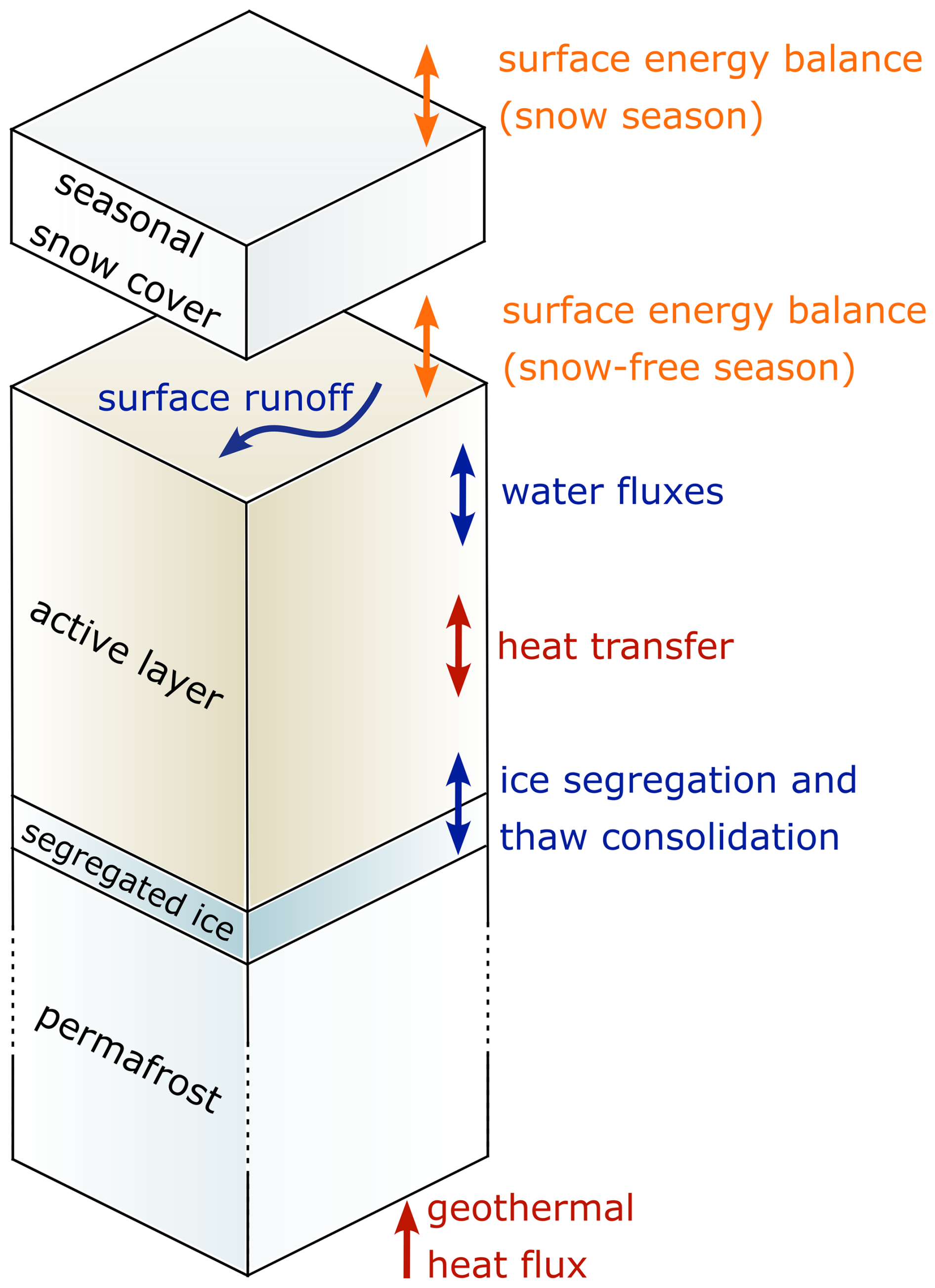
Figure 1 The main functionalities of the CryoGrid community model include the surface energy balance at the ground-atmosphere interface (snow-free season) and the snow-atmosphere interface (snow season), surface runoff, subsurface water fluxes based on Darcy's law and Richard's equation, conductive and convective heat transfer, ice segregation and thaw consolidation as well as a geothermal heat flux as lower boundary condition.

2.1.2 Thawing Slope Stability Index TSSI

The existing model functionalities are extended to represent the processes associated with slope failures in ice-rich permafrost, specifically active layer detachment failures (ALDF). Slope stability is typically evaluated based on a factor of safety F_s, which is the ratio of shear strength τ [Pa] and shear stress τ_mob [Pa] on the potential failure plane (Salunkhe et al., 2017):

$$\begin{array}{}\text{(3)}& F_{\mathrm{s}}={\displaystyle \frac{\mathit{\tau }}{{\mathit{\tau }}_{\text{mob}}}}\end{array}$$

The shear stresses, τ_mob [Pa], are induced by gravity, depending on the total stress, σ_z [Pa], and the slope angle β [–] (Lewkowicz and Harris, 2005):

$$\begin{array}{}\text{(4)}& {\mathit{\tau }}_{\text{mob}}={\mathit{\sigma }}_z\sin \left(\mathit{\beta }\right)\cos \left(\mathit{\beta }\right).\end{array}$$

The shear strength is calculated based on the Mohr-Coloumb failure criterion. It is controlled by the normal stress on the potential failure plane σ_n [Pa], the pore water pressure u [Pa] and the effective shear parameters of the soil, namely, the effective angle of internal friction ϕ^′ [rad] and the effective cohesion c^′ [Pa]. The difference of normal stress and pore water pressure can be expressed as the effective stress ${\mathit{\sigma }}_z^{\prime }$ [Pa], projected onto the terrain with the slope angle β [rad]. The shear strength τ [Pa] is calculated according to Lewkowicz and Harris (2005):

$$\begin{array}{}\text{(5)}& \mathit{\tau }=\left({\mathit{\sigma }}_{\mathrm{n}}-u\right)\tan \left({\mathit{\varphi }}^{\prime }\right)+c^{\prime }={\mathit{\sigma }}_z^{\prime }{\cos }^{\mathrm{2}}\left(\mathit{\beta }\right)\tan \left({\mathit{\varphi }}^{\prime }\right)+c^{\prime }.\end{array}$$

In unfrozen conditions, the model assumes constant values for the effective angle of internal friction ϕ^′, dependent on the soil type. In this study, we account for changes upon freezing, following the approach of Nater et al. (2008), and calculate the effective angle of internal friction in a frozen state ${\mathit{\varphi }}_{\text{frozen}}^{\prime }$ depending on the volumetric ice content θ_i:

$$\begin{array}{}\text{(6)}& {\mathit{\varphi }}_{\text{frozen}}^{\prime }={\mathit{\varphi }}^{\prime }-{\mathit{\varphi }}^{\prime }{\mathit{\theta }}_{\mathrm{i}}^{\mathrm{2.6}}.\end{array}$$

The effective cohesion c^′ in frozen conditions is controlled by the volumetric ice content and the ground temperature: the model first calculates the cohesion for the given volumetric ice content θ_i at a ground temperature T_g of −2.1 °C

$$\begin{array}{}\text{(7)}& c^{\prime }\left(T_{\mathrm{g}}=-\mathrm{2.1}\mathrm{°}\mathrm{C}\right)=\mathrm{534.93}{\mathit{\theta }}_{\mathrm{i}}^{\mathrm{1.91}},\end{array}$$

before adapting it to the actual ground temperature T_g

$$\begin{array}{}\text{(8)}& c_{\text{frozen}}^{\prime }={\displaystyle \frac{-c_{\text{frozen}}^{\prime }\left(T_{\mathrm{g}}=-\mathrm{2.1}\mathrm{°}\mathrm{C}\right)}{\mathrm{2.1}}}{T}_{\mathrm{g}}.\end{array}$$

The factor of safety F_s is then computed for all grid cells in the soil column and at every time step of the simulation period.

In the field, failure may not occur at an F_s of unity calculated from an infinite slope analysis since geocryological and topographic conditions are heterogeneous. Moreover, in the model, unstable conditions can involve multiple connected grid cells and may persist for several time steps. To take both the severity and the duration of potentially unstable conditions into account, the model assesses the Thawing Slope Stability Index (TSSI) which integrates the simulated factor of safety F_s over all consecutive time steps with unstable conditions:

$$\begin{array}{}\text{(9)}& \mathrm{TSSI}=\underset{t_{\mathrm{1}}}{\overset{t_{\mathrm{2}}}{\int }}\text{max}\left(\mathrm{1}-F_{\mathrm{s}}\left(t^{\prime }\right),\mathrm{0}\right)\mathrm{d}{t}^{\prime }\end{array}$$

The TSSI, therefore, indicates the cumulative duration and magnitude of risk for slope failure based on the physical processes of thaw active in the ground.

2.2 Study area

We applied the slope stability assessment computed by the CryoGrid geomechanical scheme to an area of approximately 2300 km² on Banks Island, Canada in the continuous permafrost zone (Brown et al., 1997, Fig. 2a, b). The study area forms part of the Jesse Moraine belt in the southeast of the island which is characterized by sediment-rich ground ice of glacial origin, overlain by 1–2 m of glacial till (Lakeman and England, 2012), in which ground ice contents are estimated to 50 %–55 % (French, 2017). The terrain is gently undulating (French, 2017) with a vegetation cover of herbs, lichen and dwarf shrubs, typically less than 5 cm tall (Raynolds et al., 2019).

Banks Island has a cold and dry climate (Vincent, 1982). The mean annual air temperature at Sachs Harbour (71.99° N, 125.24° W), about 150 km west of the study area, is −12.1 °C (1991–2020), with the average monthly temperature ranging from −27.4 °C in January to 6.5 °C in July (Government of Canada, 2025). Annual precipitation is about 140 mm with rainfall restricted to the summer months. Snowfall can occur throughout the year (Government of Canada, 2025), but the typical winter snowpack is relatively thin due to sublimation and wind redistribution, except where snow accumulates in topographic hollows (French, 2017).

The permafrost thickness on Banks Island is estimated to be 300–500 m (French, 2017) and ground temperatures in the northern part of the island averaged −12.2 °C at both 0.5 and 2.0 m depths (2011–2018) (Permafrost Laboratory/University of Fairbanks, 2025). Evidence of slope instability, especially in the form of RTS but also as ALDF, are concentrated in areas where buried ice or large ice wedges are present within 25–50 km of the coast in the southwestern, eastern and northern parts of the island (French, 1974; Lewkowicz, 1987; Fraser et al., 2018). Lewkowicz and Way (2019) present a long-term record of more than 4500 RTS initiated on Banks Island between 1985 and 2015, mainly in association with four warm summers. Of these, 849 are located within the study area (Fig. 2b).

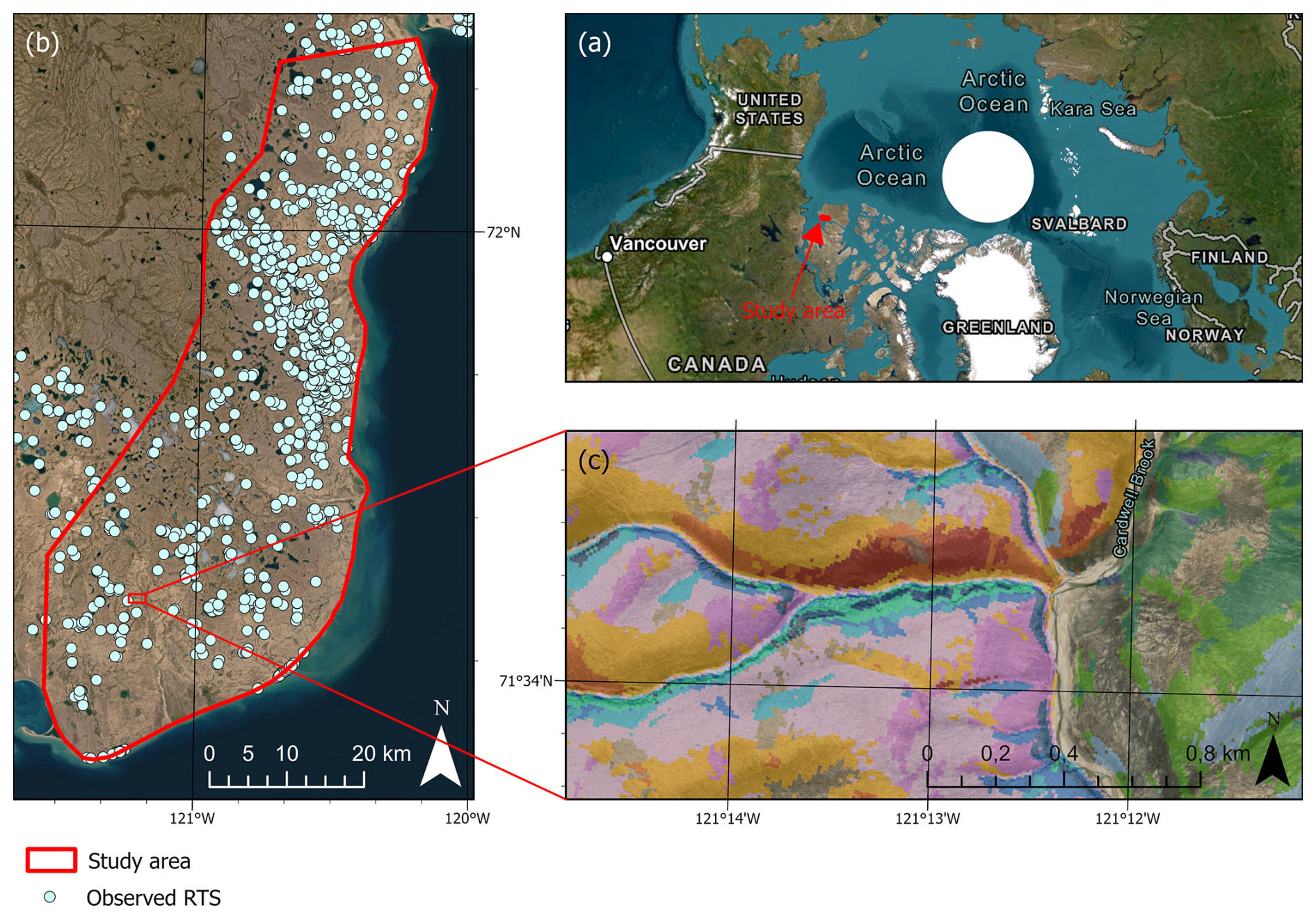
Figure 2 (a) Location of the study area, southeast Banks Island, Canada. (b) The study area (red outline) covers approximately 2300 km² and includes more than 800 RTS initiated between 1985 and 2015 (Lewkowicz and Way, 2019). (c) An example of slope clustering based on slope angle and aspect: north-facing slopes are blue, east-facing slopes are pink, south-facing slopes are red and west-facing slopes are green, with colour intensity varying with slope angle. Areas with slope angles < 2° are not shaded. Sources: Esri, TomTom, Garmin, FAO, NOAA, USGS, © OpenStreetMap contributors, and the GIS User Community | Powered by Esri.

2.3 Clustering and model forcing data

The topography of the study area was extracted with a resolution of 10 m from the ArcticDEM (Porter et al., 2023). To identify typical slope angles and aspects, we applied k-means clustering, and subsequently performed simulations only for these clusters (Fiddes and Gruber, 2012). Given the terrain (95 % < 350 m above sea level), it was not necessary to account for differences in elevation and 20 clusters were sufficient to represent the variability in slope angle and aspect. Slope failures in ice-rich soils can be found over a wide range of slope angles (Nesterova et al., 2024) but they typically occur on slopes steeper than 2° (Niu et al., 2016; Rudy et al., 2017; Mu et al., 2020; Leibman et al., 2023). For computational efficiency, we included only the portion of the study area (69.6 %) that met this criterion. This was represented by the 20 clusters which individually covered between 0.5 % and 6.2 % of the area with slope angles ranging from 2.9 to 16.0° (Fig. 2c).

To run the model, we prepared a forcing time series based on the ERA5 reanalysis (Hersbach et al., 2020) from 1950 to 2022. We used the ERA5 grid cell for Sachs Harbour (71.99° N, 125.24° W) as a proxy for the study area. This was done to reduce the potential impact of small-scale and highly variable sea ice conditions in the Amundsen Gulf on the ERA reanalysis (Galley et al., 2008; Renfrew et al., 2021), and to allow an assessment of the performance of the data set. The R² value, the root mean squared error RMSE and the bias b showed good agreement between the Sachs Harbour station data and ERA5 for mean monthly values in all seasons (R² = 0.99, RMSE = 1.2 °C, b= 0.6 °C) and for the summer months of July and August (R² = 0.97, RMSE = 0.5 °C, b = 0.1 °C), including a good representation of extreme summers.

We downscaled the radiation terms of the ERA5 data for each cluster, based on the slope angle and aspect. We followed the approach of Fiddes and Gruber (2014), which has been integrated into the CryoGrid community model (Schmidt et al., 2021). The steps involved separating the short-wave radiation into its direct and diffuse components. The direct short-wave radiation was then projected onto the given slope, while the diffuse short-wave radiation was adjusted based on the sky view factor. The long-wave radiation was corrected by reducing it according to the same sky view factor and adding the long-wave emissions from the surrounding terrain, assuming its temperature to be that of the air.

The simulation was conducted for the entire time period of 1950 to 2022 with the first 10 years as model spin-up, using the accelerated spin-up procedure described in Westermann et al. (2023).

2.4 Model parameterization

The model domain extended to a depth of 100 m, with the slope stability assessment undertaken for the top 9 m using the CryoGrid geomechanical scheme, i.e. the stratigraphy class GROUND_freezeC_RichardsEq_seb_pressure. The upper 0.05 m of the ground was characterized by an organic layer, with 20 % organic material and 20 % mineral content (initial void ratio of 1.5; Table 1), representing the vegetation assemblages found on Banks Island (French, 2017). The glacial till beneath was set to 50 % ground ice content and 50 % mineral content (initial void ratio of 1.0), following French (2017) who estimates ground ice contents of about 50 %–55 %. This stratigraphy was compressed during initialization based on the stress conditions in the soil, resulting in 50 % porosity in the organic layer and 46 % porosity on average in the glacial till, with the pore space decreasing with depth. To account for buried and wedge ice which can be present at depths of 1 m or more (Lakeman and England, 2012), we assigned a total volumetric ground ice content of about 80 % below 1 m depth. This is in line with the ground ice map of Canada, which modeled excess ice contents greater than 30 % for the Jesse moraine in addition to pore ice (O'Neill et al., 2022).

Table 1 The soil stratigraphy for the upper 9 m of the model domain after initialization, consisting of an organic layer at the top and the glacial till below. θ_m: volumetric fraction of mineral content; θ_o: volumetric fraction of organic content; θ_wi: total volumetric fraction of water and ice content; S: saturation; e₀: initial void ratio before compaction; σ₀: residual stress; C_c: compression index; ϕ^′: effective friction angle in unfrozen conditions; k_w: permeability; α: alpha coefficient; n: n coefficient.

Westermann et al. (2016)Zweigel et al. (2021)Westermann et al. (2016)Westermann et al. (2016)Westermann et al. (2023)Zweigel et al. (2021)Westermann et al. (2023)Zweigel et al. (2021)Barrere et al. (2017); Royer et al. (2021)Westermann et al. (2023)

Table 2 Model parameters and settings.

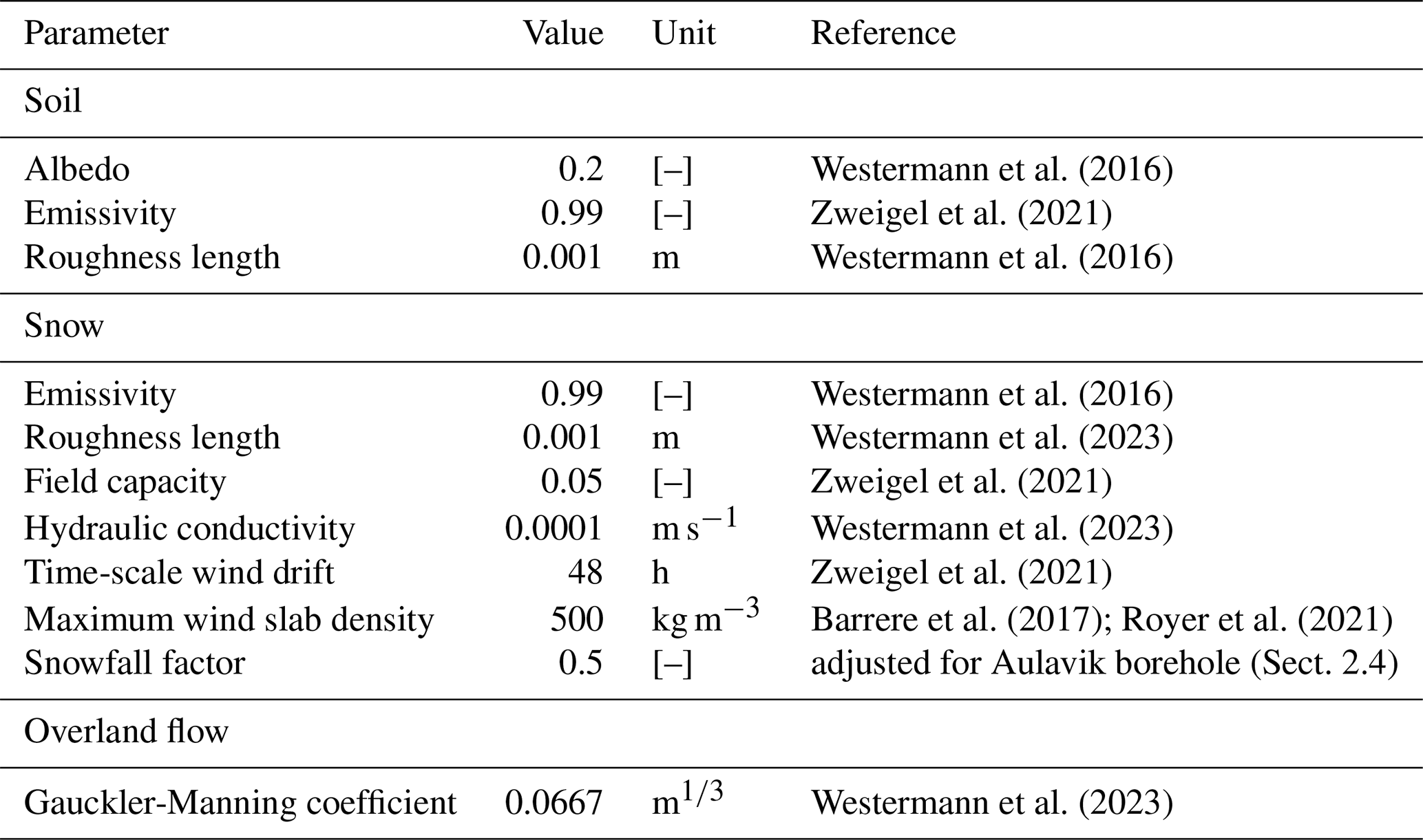
Values for the residual stress σ₀, compression index C_c, and van Genuchten parameters α and n were adapted from Aga et al. (2023), following established literature (Van Genuchten, 1980; Gudehus, 1981; Dall'Amico et al., 2011; Dumais and Konrad, 2018, 2019). The effective angle of internal friction ϕ^′ for the glacial till was set to 20° during unfrozen conditions, which is in line with literature values (Prinz and Strauß, 2012). A surface albedo of 0.2, an emissivity of 0.99, and an aerodynamic roughness length of 0.001 m were employed during the snow-free season, as in Aga et al. (2023) (Table 2).

We did not account for soil mechanical processes at depths greater than 9 m as the soil remained frozen throughout the simulation. We set the volumetric mineral content to 0.7, the volumetric ice content to 0.3 and applied the simplified stratigraphy class GROUND_freeW_seb, enabling more efficient computations for these greater depths (Westermann et al., 2023).

The seasonal snow cover was represented by the stratigraphy class SNOW_crocus2_bucketW_seb (Westermann et al., 2023). The maximum wind slab density was set at 500 kg m⁻³, based on Barrere et al. (2017) and Royer et al. (2021). Further parametrization for the snow class can be found in Table 2. Standing surface water was removed by overland flow, following the Gauckler-Manning equation (Gauckler, 1867; Manning et al., 1890), for which we set the Gauckler-manning coefficient to 0.0667 m${}^{\mathrm{1}/\mathrm{3}}$ (Table 2). Lateral water fluxes in the ground and snowpack were not included in the model setup.

The grid cell size generally increased with depth, but the lowermost part of the active layer and the uppermost part of the permafrost were simulated using the finest vertical discretization, as this was the critical part for slope stability. The grid cell sizes were: 0–0.5 m depth: 0.05 m; 0.5–1.3 m depth: 0.025 m; 1.3–2 m depth: 0.05 m; 2–4 m depth: 0.1 m; 4–20 m depth: 0.25 m; 20–50 m depth: 1 m; 50–100 m depth: 5 m.

To assess the performance of the ground thermal modelling for the study area, we ran the model for a site in Aulavik National Park, where ground temperature data from a borehole was available from 2010 to 2018 (Permafrost Laboratory/University of Fairbanks, 2025), based on ERA5 data for this location. A snowfall factor of 0.5 was necessary to achieve a good fit with observed winter temperatures (Appendix A). The same snowfall factor was then applied to the study area in southeastern Banks Island where no observations were available. This relatively low snowfall factor can be explained by snow sublimation and significant wind redistribution which results in snow accumulations in topographic hollows, while the uplands typically exhibit little to no snow cover (Sect. 2.2; French, 2017). The model would also allow to cluster the field area by snowfall factor, in addition to slope angle and aspect, for example based on satellite imagery. However, we applied a constant snowfall factor for simplicity, as the snowpack is typically thin on Banks Island due to sublimation and wind redistribution (French, 2017).

2.5 Model validation

The model represents the processes resulting in active layer detachment failures (ALDF), however, no inventory of ALDF was available to support a statistical analysis of their occurrence. Therefore, we used a long-term inventory of newly initiated retrogressive thaw slumps (RTS) for validation (Lewkowicz and Way, 2019). The observed peaks in RTS initiation were associated with exceptionally warm summers and a deepening of the active layer. Lewkowicz and Way (2019) point out that the main trigger of RTS in the field area was ALDF exposing massive ground ice, while fluvial, lacustrine and coastal erosion may have acted as pre-conditioners to RTS initiation but cannot explain the high numbers of newly initiated RTS within the same year. Consequently, the RTS database can be used as a proxy for ALDF.

3 Results

3.1 Simulated permafrost conditions

We simulated permafrost conditions for the study area between 1950 and 2022, which included the time period of the long-term RTS inventory that we used for comparison (1984–2015) (Lewkowicz and Way, 2019). In the first 55 years (1950–2005), simulated mean annual ground temperatures (MAGT) at 2 m depth slowly increased, varying between −12.9 and −10.1 °C, with the exceptions of 1998 and 1999 when higher ground temperatures of −9.5 and −9.7 °C, respectively, were simulated (Fig. 3). In the 16 years between 2006 and 2022, in contrast, simulated ground temperatures were higher due to climate warming, varying between −10.3 and −8.8 °C. The MAGT at 2 m depth varied little among the clusters with a maximum difference of 0.15 °C, indicating that aspect and slope angle have only a minor influence on annual ground temperatures.

The active layer thickness (ALT) ranged between 0.50 and 1.00 m during the simulation period (Fig. 3). The overall trend was for a slight increase in ALT but this was accompanied by considerable interannual variability. For example, shallow active layers were modelled both near the beginning (e.g., 1967) and near the end of the time period (e.g., 2019), and the same applies to deep active layers (e.g., 1988 and 2022). In several years, a deep active layer thawed into the excess ice layer (Fig. 3). In contrast, differences in ALT among the clusters were minor, with 1 cm on average, and 2 cm as the maximum value. This can be explained by a lower percentage of direct short-wave radiation (45 %) compared to diffuse short-wave radiation (55 %) with the latter being independent on the orientation of the slope. It should be noted that the model does not include long-term feedbacks between soil moisture and vegetation cover which could affect ALT.

The volumetric water and ice content θ_wi in the upper 1 m of the soil column had a mean value of 31 %, but exhibited annual fluctuations, following variations in the soil moisture content of the active layer (Fig. 3). In contrast, θ_wi in the excess ice layer remained relatively stable at approximately 81 %, with fluctuations occurring primarily in the uppermost few centimeters near the permafrost table. When the active layer thawed into the excess ice layer, the excess ice melted and θ_wi decreased as the liquid water was mobilized and routed to higher grid cells during thaw consolidation. For example, a deep active layer melted 3.0 cm into the excess ice layer in 2012, corresponding to 2.4 cm of lost ground ice. During the following 3 years, which were characterized by lower ground temperatures (Fig. 3), 0.8 cm of excess ice again formed at the top of the permafrost through ice segregation.

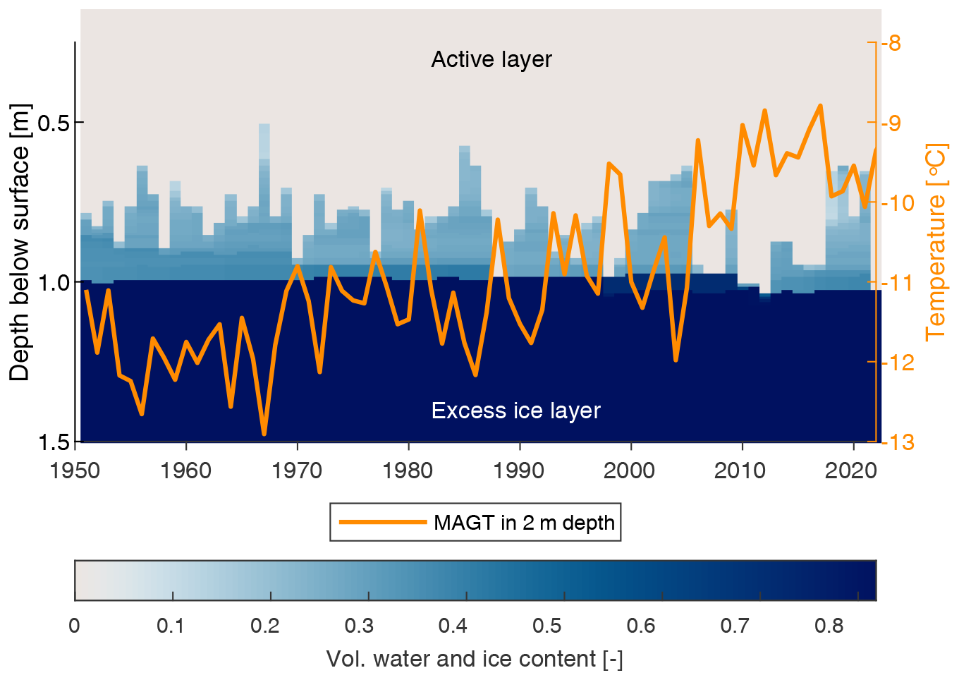
Figure 3 Simulated mean annual ground temperature (MAGT) at 2 m depth and minimum annual volumetric water and ice content (1950–2022). The latter is only shown for grid cells with continuously frozen conditions for the respective year to visualize the depth of the active layer. Both parameters are the average values for the 20 clusters weighted by cluster area.

3.2 Assessment of ground stability

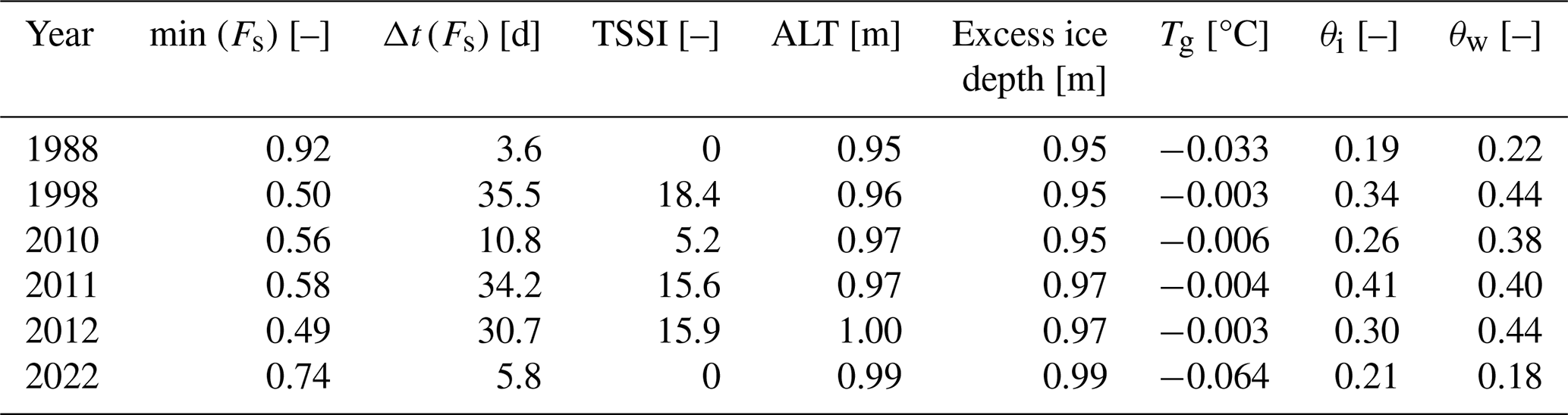
Potentially unstable conditions with F_s < 1 were simulated for eight of the 43 years: 1954, 1970, 1988, 1998, 2010, 2011, 2012, and 2022 (Table 3). While the first two were caused by melting of segregated ice layers within the active layer, which were formed by the model in preceding years (Sect. 2.1.1), all unstable conditions since 1988 resulted from thawing into the pre-assigned excess ice layer which represents buried and wedge ice (Sect. 2.4). Therefore, we restricted the further analysis to the time period 1980 to 2022.

The lowest factor of safety min (F_s) of 0.49 was modelled for 2012, and the longest period of unstable conditions Δt(F_s) of 35.5 d was in 1998. The years with unstable conditions were characterized by high summer (July–August) air temperatures and intense short-wave radiation (Fig. 5). While air temperature (short-wave radiation) averaged 5.3 °C (169 W m⁻²) between 1980 and 2022, values in years with simulated unstable conditions were between 7.3 and 8.8 °C (178 and 194 W m⁻²). In contrast, no obvious correlation of unstable conditions with precipitation or long-wave radiation could be identified from the simulations.

High summer air temperatures and intense short-wave radiation resulted in a deepening of the active layer in the model, extending into the excess ice layer during years with unstable conditions (Fig. 3). The deepest thaw was simulated in 2012 (Table 3). Unstable conditions were mainly simulated to occur in the uppermost excess ice layer, in which ground temperatures were just below 0 °C and where ground ice coexisted with liquid soil water (Table 3). An example is illustrated in Fig. 4, showing that the unstable conditions occur at the top of the permafrost. In this zone, the presence of ice caused a drastic reduction in hydraulic conductivity: while the lowest unfrozen grid cell in the active layer had simulated hydraulic conductivities of 1.5 × 10⁻⁸ to 3.2 × 10⁻⁸ m s⁻¹, the unstable grid cells with coexisting ground ice and liquid water exhibited much lower values of 5.6 × 10⁻¹² to 8.5 × 10⁻¹¹ m s⁻¹. This strong reduction in hydraulic conductivity restricted the drainage of meltwater into the unfrozen active layer, even when the active layer itself was not fully saturated, thereby promoting excess pore water pressures. A low minimum factor of safety min (F_s) and a long period of unstable conditions Δt(F_s) occurred when the ground temperatures were closest to 0 °C, in conjunction with high volumetric soil water contents. This was the case for the years 1998, 2010, 2011, and 2012, with min (F_s) between 0.49 and 0.58, and Δt(F_s) ranging from about 10.8 to 35.5 d. Although instability was simulated for 1988 and 2022, min (F_s) were higher (0.92 and 0.74, respectively), and Δt(F_s) was shorter (3.6 and 5.8 d, respectively).

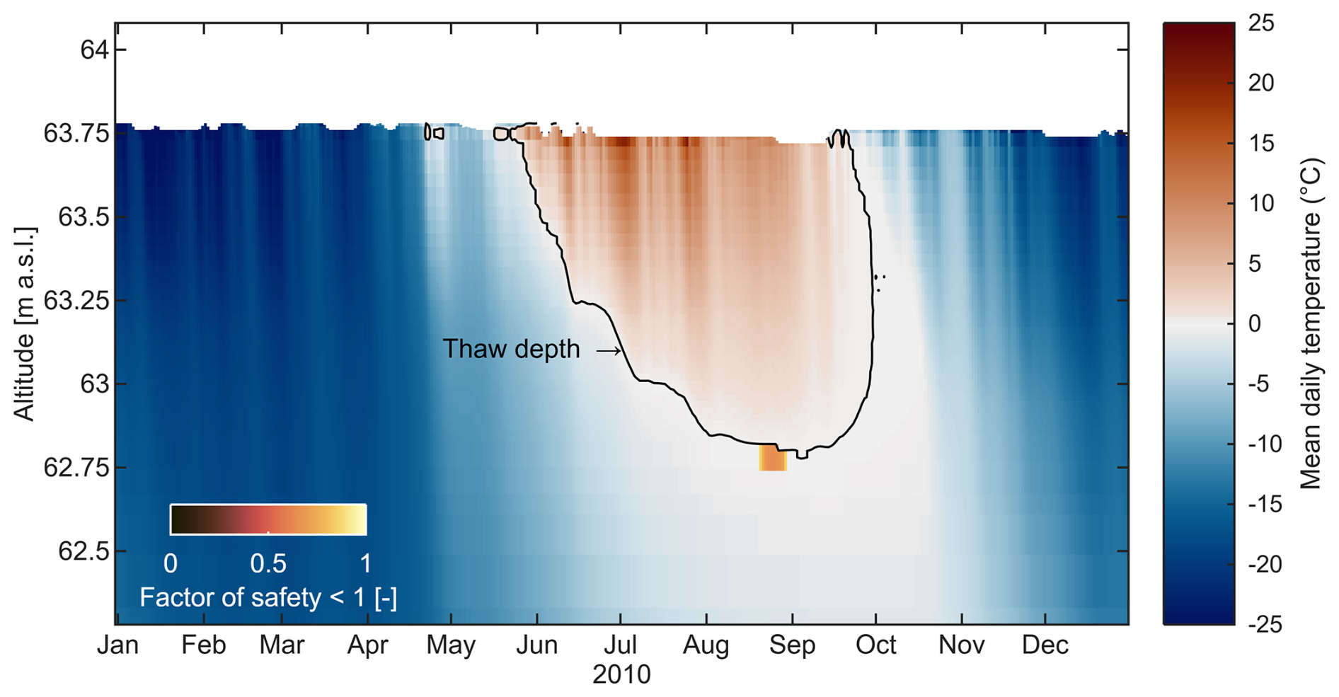
Figure 4 Simulated mean daily ground temperature in 2010 for a cluster with a north-facing slope and a slope angle of 3.4 °. The figure illustrates that unstable conditions occur at the top of the permafrost, where ground temperatures are just below 0 °C.

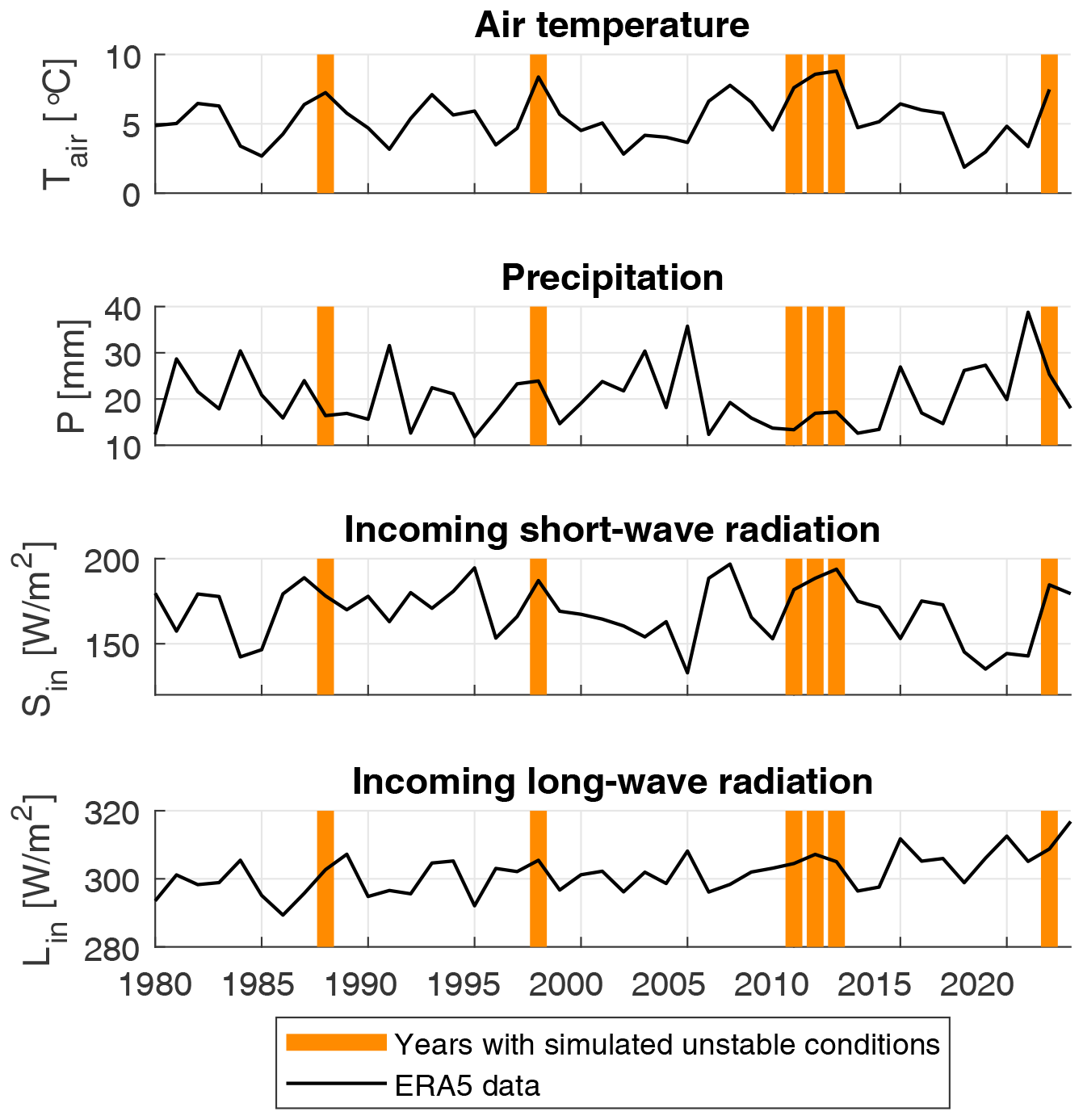
Figure 5 Climatic conditions during summer (July–August, 1980–2022) based on ERA5 data and years with simulated slope instability. Note: incoming short-wave and long-wave radiation are for horizontal surfaces.

Table 3 Years with simulated unstable conditions. Given are the minimum factor of safety min (F_s), the duration of unstable conditions Δt(F_s), the median Thawing Slope Stability Index TSSI, the active layer thickness ALT, and the depth of the excess ice layer before the summer season. Ground temperature T_g, ice content θ_i and water content θ_w in the unstable part of the ground column are also shown. All parameters are the average values for the 20 model realizations representing the clusters, weighted by the cluster area.

3.3 Susceptibility to slope failure

3.3.1 Temporal evolution of the TSSI

Median TSSI (Thawing Slope Stability Index) was calculated for all years, weighted by the cluster area. Years with stable conditions had a TSSI of 0, whereas those with unstable conditions had a positive TSSI. The modelling produced a range of values across the study area with positive median TSSI of 5.2–18.4 for 1998, 2010, 2011, and 2012 (Table 3 and Fig. 6a), indicating a high likelihood of ALDF. Other years with unstable conditions (1988, 2022) had very low values of TSSI (median TSSI of zero), indicating that slope failure was likely only in certain slope clusters.

We compared the model results with a database of newly observed RTS (Lewkowicz and Way, 2019). The database showed no or only isolated incidents of RTS initiation in most years, but four had exceptionally high counts: 1999 (483 RTS), 2011 (49 RTS), 2012 (188 RTS), and 2013 (48 RTS) (Fig. 6a). However, Lewkowicz and Way (2019) point out that RTS are not necessarily detected in the actual year of initiation (only 33.3 % of RTS on Banks Island) but more frequently in the year after (66.7 %). That explains why high TSSI values were typically simulated one year earlier than the observed RTS (Fig. 6a).

Motivated by the characteristics of the observations, we weighted the TSSI following Lewkowicz and Way (2019), assigning 33.3 % to the year of RTS observations, and 66.7 % to the preceding year, before comparing it to the observational data (Fig. 6b). There is a log-linear relationship between the weighted TSSI and the number of newly observed RTS. All years without observed RTS were simulated with a TSSI of 0, indicating no susceptibility to slope failure. For years with a high number of newly observed RTS, we simulated a high value of the weighted TSSI, such as in 1999 (483 RTS, weighted TSSI = 12.3), 2011 (49 RTS, weighted TSSI = 8.7), 2012 (188 RTS, weighted TSSI = 15.7), and 2013 (48 RTS, weighted TSSI = 10.6). Some years with observations did not have positive modelled TSSI, but these were years with 11 or less newly initiated RTS over an area of about 2300 km². Such small numbers may have been triggered by local factors such as river or coastal erosion, and thus cannot be captured by the model, or they may represent inaccuracies in the interpreted timing of RTS initiation.

The number (483) of newly observed RTS in 1999 appeared large when compared to the TSSI of 12.3 weighted between 1998 and 1999. A better fit was obtained using the TSSI for 1998 alone (18.4) (Fig. 6b). This suggests that most of this group of RTS were identified in the year following their initiation, possibly as a result of the imagery for 1998 dating earlier in the thaw season than the timing of RTS initiation (Lewkowicz and Way, 2019).

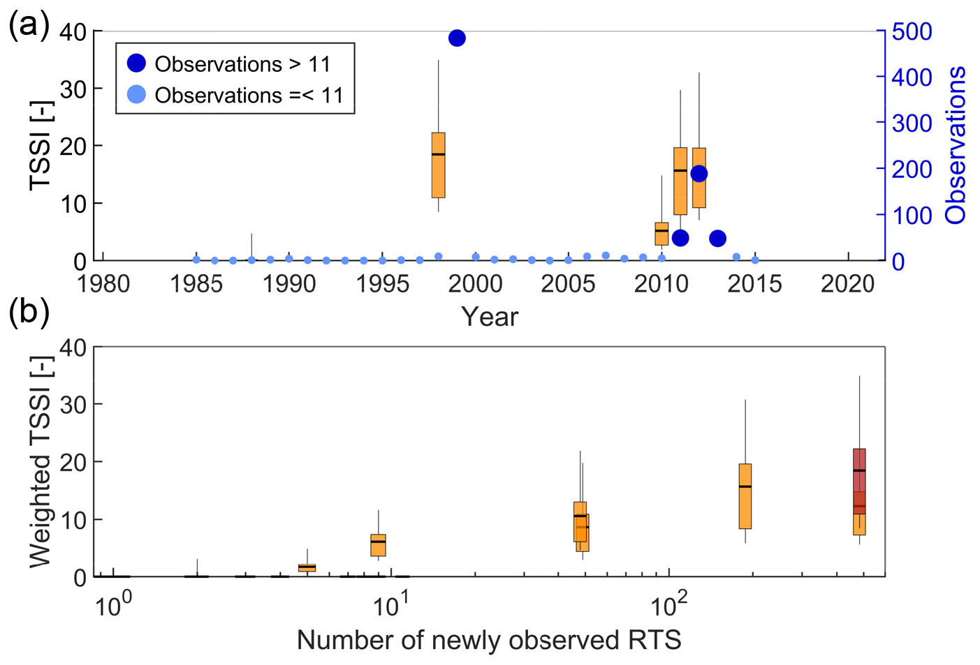
Figure 6 (a) Simulated TSSI (1980–2022) and the number of newly observed RTS in the study area (1985–2015). Many new RTS are detected in the satellite imagery in the year following their initiation (Lewkowicz and Way, 2019), explaining the time lag with the TSSI. (b) Log-linear relationship between weighted TSSI (taking into account the time lag – see text) and the number of newly observed RTS in the study area. The TSSI relating to the highest number of RTS in 1999 is shown as weighted between the years of 1998 and 1999 (orange) and entirely based on 1998 (red).

3.3.2 Spatial variability of the TSSI

The clustering procedure (Sect. 2.3) allowed the effect of slope angle and aspect to be explored for the years with positive TSSI. The slope angles within the clusters ranged from 2.9 to 16.0° with a median of 4.8°, reflecting a terrain primarily characterized by gentle hills. In the years with unstable conditions, the highest TSSI was simulated on the steepest slopes, which are prevalent in all cardinal directions (Fig. 7a). The relationship between TSSI and slope angle is positive curvilinear as illustrated in Fig. 7b. Substantial changes occurred in TSSI at low slope angles while further increases in angle on steeper slopes had less impact. TSSI values were highest on all slopes in 1998.

The relationship between TSSI and aspect is weak (Fig. 7a, c). High susceptibility occurs across all cardinal directions, and TSSI varies substantially even among similar aspects (e.g., east-facing slopes). This variability is primarily controlled by slope angle (through the occurrence of steep slope in all cardinal directions), which exerts a stronger influence than aspect and thus masks any aspect-related signal. The weak dependency on aspect is also evident in the observed RTS: 25 % are north-facing, 41 % east-facing, 18 % south-facing and 16 % west-facing (each defined as the cardinal direction ± 45°). This distribution reflects well the peaks in TSSI shown in Fig. 7c. To reduce the masking effect of steep slope angles, Fig. 7d restricts the analysis to gentle slopes (< 4°), which reveals that the highest values for TSSI are found for east- and south-facing slopes, aligning with the expected impact of increased solar irradiation.

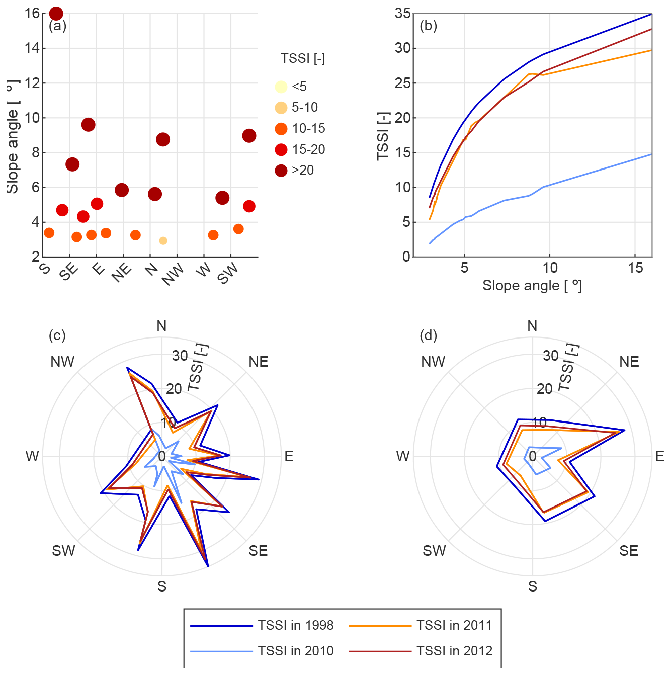
Figure 7 Relationship between the simulated TSSI and (a) slope angle and aspect in the year 1998, (b) slope angle, (c) aspect and (d) aspect for clusters with slope angles < 4°. Note: Years with a mean TSSI of zero are not shown.

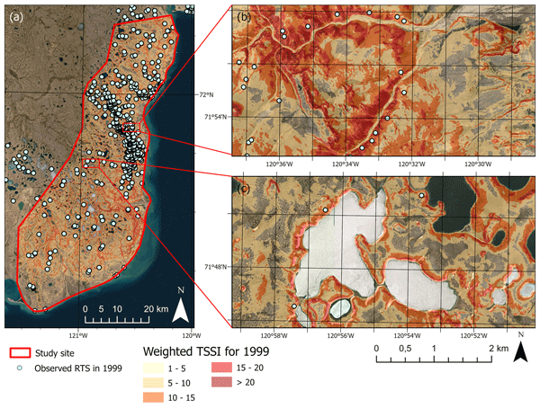
Based on the clustering approach (Sect. 2.3), it is possible to output the annually modelled TSSI as a series of maps for the study area. Years with stable conditions, such as for example the year 2000, do not show any TSSI above zero and appear completely transparent. In contrast, the TSSI map for 1999 (weighted 66.6 % to 1998 and 33.3 % to 1999) shows a substantial susceptibility to slope failure for large parts of the study area (Fig. 8a). The highest and most widespread TSSI was simulated along the rivers (Fig. 8b), but high TSSI values were also modelled around lakes (Fig. 8c) and on other slopes with steep slope angles (Fig. 8b). This spatial distribution is in agreement with the database of Lewkowicz and Way (2019), in which 75 % of the 483 newly initiated RTS were observed along rivers, while 15 % occurred around lakes, 3 % at the coastline and 7 % on other slopes.

We validated the map by calculating the landslide density LD (Pham et al., 2016), i.e., the ratio of the percentage of landslide pixels in the entire study area and the percentage of landslide pixels in the respective TSSI classes shown in Fig. 8. The landslide density shows the following distribution: LD (TSSI < 5) = 0.2, LD (5 < TSSI < 10) = 0.9, LD (10 < TSSI < 15) = 1.7, LD (15 < TSSI < 20) = 2.5 and LD (20 < TSSI) = 14.7. This confirms that the RTS on Banks Island were predominantly initiated in areas with a high simulated TSSI, particularly in areas with a TSSI above 20.

Some discrepancies remain between the spatial distribution of simulations and observations. The southeastern part of the study area, for example, is characterized by relatively steep slopes where high weighted TSSI values were computed for 1999, but few RTS were initiated (Fig. 8a). This may be the result of a heterogeneous distribution of ground ice in the field that is not represented in the model. The study area is mapped at the national scale as having high abundance of relict ice and medium abundance of segregated ice (O'Neill et al., 2019), but the area in the southeast shows a low abundance of ice wedges compared to medium or high abundance in the rest of the study area (O'Neill et al., 2019). It is therefore possible, that the ground ice content, which was set in the model to be uniform across the study area, is actually lower in the southeastern part, resulting in a local overprediction of the TSSI. As often pointed out in landslide literature, accurate predictions of slope instability are subject to detailed knowledge of subsurface conditions.

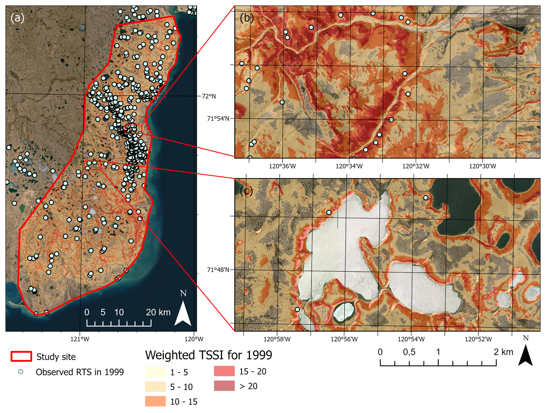
Figure 8 The simulated weighted Thawing Slope Stability Index (TSSI) and newly observed initiated retrogressive thaw slumps (RTS) in 1999 for the entire study area. Sources: Esri, TomTom, Garmin, FAO, NOAA, USGS, © OpenStreetMap contributors, and the GIS User Community | Powered by Esri.

4 Discussion

4.1 Capabilities of the new model scheme

This study advances the field in four main ways. First, it demonstrates that the geomechanical model that was incorporated in the CryoGrid community model by Aga et al. (2023) can be used within an infinite slope analysis to predict potential slope instability, which may lead to the initiation of ALDF and potentially RTS when triggered by exposure of massive ice through ALDF. This permits physically-based spatial modelling of the factor of safety for permafrost slopes using inputs of meteorological variables and subsurface soil and geocryological information. Since the model is not empirically or statistically based, it could be applied to any permafrost environment for which cryostratigraphies are available.

Second, it develops the TSSI which incorporates both the degree of instability and its duration. While previous studies focused on the factor of safety for individual permafrost slopes (Chandler, 1972; Hutchinson, 1974; Lewkowicz and Harris, 2005; McRoberts and Morgenstern, 1974; Zhang et al., 2022), the TSSI computation is based on key physical processes contributing to unstable conditions, such as stress conditions throughout the soil column, water fluxes that promote ice segregation and thaw consolidation, and the factor of safety. Representing the topography by clustering proved essential because slope angle and to a limited extent also aspect influence the TSSI. The slope angle appears in the equations to calculate the factor of safety and thus determines the TSSI. Aspect affects the TSSI indirectly by controlling the ground temperatures and active layer thickness, especially through differences in incoming short-wave radiation. The weak dependence on aspect indicates that variability in thaw-driven slope instability on Banks Island is only little influenced by differences in short-wave radiation, consistent with the similar weak signal in the observational data. In landscapes with steeper terrain and stronger topographic shading, however, the influence of aspect is likely to be more pronounced. But also the relatively small effect in the gently undulating terrain of Banks Island underscores the importance of slope angle and aspect when assessing susceptibility to slope failure.

Third, the validity of the TSSI as an indicator of slope instability was demonstrated by comparing it to a long-term inventory of newly observed RTS (Lewkowicz and Way, 2019). The occurrence of new RTS peaked in warm summers, since the main trigger of RTS in this field area were thaw-driven ALDF exposing massive ice (Lewkowicz and Way, 2019). The database is therefore a suitable proxy for ALDF occurrence (Sect. 2.5). A log-linear trend was evident between weighted TSSI and the number of new RTS, suggesting that the model is capable of reconstructing and potentially predicting conditions where slope failure in ice-rich permafrost is likely. Furthermore, areas with a high TSSI featured an increased landslide density, showing that the model could identify the slopes with the highest susceptibility to failure.

Finally, the successful implementation and validation of the new model scheme opens the door to predictive modelling. By integrating our approach into the CryoGrid community model, it is possible for the first time to simulate the dependency of unstable conditions on climatic conditions, allowing an assessment of the susceptibility to slope failure over large spatial scales and long time periods including past and future climates. The example presented from Banks Island shows that years with high summer air temperature and high incoming short-wave radiation in summer resulted in unstable conditions and the formation of RTS, while precipitation and thus the degree of saturation in the active layer played a minor role at this field area. The model results show that unstable conditions can be traced back to high pore water pressures, which build up when the drainage of liquid water is restricted by clogging of the pathways by coexisting ground ice. These findings are in line with Dai et al. (2025), who showed that temperature-driven RTS dominate over precipitation-driven RTS in high latitudes. However, the model could also be applied at field areas, where precipitation dominates the susceptibility to slope failure.

4.2 Limitations and uncertainties

A number of limitations and uncertainties in the study are linked to (1) the representation of physical processes in the model, and (2) the data available to force the model.

4.2.1 Representation of Processes

Uncertainties in the model are inherited from the CryoGrid geomechanical scheme presented in Aga et al. (2023). For example, under dry conditions, the effective stress on the soil is high, while under saturated conditions, the soil water carries some of the overburden weight, reducing the effective stress on the soil matrix. In the model, this buoyancy effect is scaled arbitrarily between 50 % saturation (no buoyancy effect) to 100 % (full buoyancy effect). This approach leads to uncertainties in the overburden pressure and thus the compression of the soil matrix, possibly affecting the pore space available for drainage of the excess melt water into the active layer. Additionally, the model does not consider the different densities of water and ice to render it compatible with other submodules in the CryoGrid community model. Therefore, the thickness of the segregated ice layers may be underestimated by about 8 %, while the amount of melt water, controlling excess pore water pressures and thus the stability of the slope, is not affected. Furthermore, the model uses a constant compression index for each soil type to calculate the relationship between effective stress and void ratio, resulting in a reversible deformation of the soil. In nature, the soil would follow the curve of the decompression index, so that the porosity after decompression is likely overestimated in the model. For further details on these uncertainties, we refer to Aga et al. (2023).

When assigning the shear strength of the soil for unfrozen and frozen conditions, we follow the approach of Nater et al. (2008). When ground ice is present, the effective angle of internal friction is reduced according to the ground ice content. In contrast, the effective cohesion increases with increasing ground ice content and decreasing ground temperature, and it becomes zero for unfrozen conditions (Sect. 2.1.2). Near-surface soils in permafrost terrain can experience strength reduction due to remoulding by solifluction processes, which may lead to a decrease in cohesion to residual values (Harris and Lewkowicz, 2000). Therefore, our parametrization for the shear strength is a conservative approximation.

Uncertainties are linked to the infinite slope analysis even though it has been previously applied to assess the stability of slopes in permafrost environments (e.g., Lewkowicz and Harris, 2005). The model assumes a planar slope of infinite extent, which rarely reflects the true complexity of natural slopes and neglects variability across or downslope (Griffiths et al., 2011). Furthermore, edge effects are not taken into account, so that the analysis should only be applied to slopes with a length $/$ depth ratio above 25 (Milledge et al., 2012), and it cannot be guaranteed that this is always the case of ALDF on Banks Island. The slope angle and aspect are determined from a DEM with 10 m resolution, so that terrain features smaller than that are not resolved. All these uncertainties lead to the conclusion that a particular slope may not fail even though its factor of safety drops below 1. We account for this by using the TSSI rather than the factor of safety for comparison with the remote sensing observations of RTS initiation.

4.2.2 Data limitations

In the model setting, we assigned constant soil properties across the study area. However, spatial variations in ground ice content and sediment characteristics exist, as shown by O'Neill et al. (2022) in relation to ground ice content and are linked to the glacial origin of the sediments (Lakeman and England, 2012). Furthermore, natural variabilities in the snow distribution likely occur due to topographical features (French, 2017). Despite the promising results achieved that reconstructed the occurrence of newly observed RTS in the area, there were local discrepancies between model results and observations. Clustering the area with land cover types, ground ice contents and different snowfall factors in addition to slope angle and aspect, could improve the model predictions. These option exists within the CryoGrid community model and their implementation is simply limited by available data. This could allow the assessment of the susceptibility to slope failure over large spatial scales, with varying subsurface properties. The depth of the excess ice layer is particularly critical as it determines whether the thaw plane reaches the excess ice during extreme summers, and thus controls the occurrence of unstable conditions.

Due to the clustering approach, a one-dimensional setup was necessary, so that lateral water fluxes in the subsurface were neglected and the same drainage conditions were applied to all grid cells. This increases the uncertainty in the model results, as lateral water fluxes can cause seepage forces that significantly reduce slope stability (Vargas Ceron et al., 2025). Theoretically, lateral fluxes could be implemented within the framework of the CryoGrid community model based on the topography, by including external water reservoirs (Westermann et al., 2023) or laterally coupled tiles (Nitzbon et al., 2019, 2020; Martin et al., 2021). However, both runoff and subsurface water flow are three-dimensional, and complex flow patterns can arise through preferential water tracks (Evans et al., 2020) or the microtopography of the frost table (Chiasson-Poirier et al., 2020). Consequently, it is a challenge to correctly set the drainage conditions over large spatial scales.

Our results show a strong link between unstable conditions and summers with high air temperatures and intense short-wave radiation. The representation of such events can be problematic in reanalysis data sets like ERA5, and accuracy can suffer at coastal locations (Sheridan et al., 2020) and in the Arctic where observing networks are sparse (Avila-Diaz et al., 2021). Furthermore, the performance of the ERA5 surface-layer meteorology over sea ice, especially over the marginal sea ice zone, is worse than over land (Renfrew et al., 2021; Pernov et al., 2024). Despite these limitations, ERA5 is one of the best reanalysis products for representing extreme air temperatures in in North America (Avila-Diaz et al., 2021). To reduce uncertainties during model testing, we used the ERA5 grid cell of Sachs Harbour as proxy for the study area, so that data could be validated against available station data, especially regarding extreme summers, which were well represented in the air temperatures (Sect. 2.3).

4.3 Outlook

As a result of the limitations and uncertainties, the model captures the susceptibility to slope failure in ice-rich permafrost, specifically ALDF, at a landscape scale but it does not predict the locations of individual events. More detailed predictions could be made, such as for each raster cell, but this would require ground ice distributions and soil properties at the same spatial resolution. Datasets at this level of detail are not generally available. Consequently, the presented model approach should be regarded as a tool to investigate the landscape-scale susceptibility to slope failures for ice-rich permafrost slopes at large temporal scales. Further testing of the model in different climatic settings and under varying ground ice and soil conditions, would be desirable to ensure its robustness.

The framework of the CryoGrid community model would allow the simulations to be extended to cover past and future climates (Aga et al., 2023; Westermann et al., 2016; Langer et al., 2024). The latter are particularly important as extreme warming events are projected to increase in continuous permafrost regions in the coming decades (Feng et al., 2025; Li et al., 2025). Such long-term assessments of susceptibility changes could complement RTS databases, including deep learning based approaches which are available for recent years with high resolution satellite imagery (e.g., Dai et al., 2025; Nitze et al., 2025). Together with field-based studies, they could provide a comprehensive perspective on the evolving risk of these slope failures in ice-rich permafrost terrain.

The presented model could be a valuable tool for further investigations of the triggers for ALDF in ice-rich permafrost environments. Disturbances within the permafrost thermal regime, such as vegetation removal (Heijmans et al., 2022) or wildfires (Lewkowicz and Harris, 2005; Jones et al., 2015; Holloway et al., 2020) can result in slope failures. These triggers could be modeled by combining the functionalities of the CryoGrid community model presented in this study with an available vegetation module of the model (Zweigel et al., 2024).

Slope failures in ice-rich permafrost have widespread environmental impacts, including on the hydrological cycle (Kokelj et al., 2021; Zhang et al., 2025), the geochemistry of the water (Malone et al., 2013), and the mobilization of sediments, solutes, and carbon (Kokelj et al., 2013; Turetsky et al., 2019), and they can pose a risk to infrastructure (Hjort et al., 2022). The mobilization of soil carbon in permafrost has been a particular focus of research as this may further increase atmospheric carbon concentrations (Schuur et al., 2008; Miner et al., 2022). Turetsky et al. (2020) estimates that hillslope erosion, including ALDF and RTS, may be responsible for one-third of abrupt carbon releases. However, uncertainties remain regarding both the initiation and expansion of these features. Therefore, it is critical to improve understanding of the susceptibility to slope failure in ice-rich permafrost at a landscape scale in unmapped areas and under future climate scenarios.

5 Conclusions

In this paper we describe the incorporation of a physically-based infinite slope analysis within the CryoGrid community model to develop a multi-decadal time series of the factor of safety for ice-rich permafrost slopes, representing the processes leading to active layer detachment failures (ALDF). The model uses meteorological data and soil freezing characteristics to calculate ground temperatures and water fluxes, and it simulates the fundamental processes of ice segregation, frost heave and thaw settlement, including the potential for high pore water pressures to develop during thaw consolidation. The model scheme is adapted to spatial analysis by clustering slope angles and aspects. The outputs include when and where in the soil profile the factor of safety falls below unity, indicating the potential for instability.

Limited data describing geocryological characteristics and the spatial heterogeneity of topography, soils and ground ice mean that a modelled prediction of instability does not necessarily indicate that a given slope will fail. Consequently, to assist with predictions, we developed the Thawing Slope Stability Index (TSSI) which takes into account the severity and duration of modelled unstable conditions. The TSSI was tested in a study area on Banks Island where hundreds of newly initiated retrogressive thaw slumps (RTS) occurred between 1985 and 2015. In this study, we use RTS initiation as a proxy for ALDF, as the exposure of massive ground ice through ALDF was reported as the main trigger for RTS initiation (Lewkowicz and Way, 2019). The newly initiated RTS developed in years with positive TSSI and were concentrated spatially in areas of the landscape with the highest TSSI values. These years were characterized by high summer air temperatures and high incoming short-wave radiation, while no dependency on precipitation or long-wave radiation could be identified. The extreme summers in the forcing data led to a deepening of the active layer and a thawing into the excess ice layer within the model. Unstable conditions were simulated in the uppermost excess ice layer, where ground temperatures just below 0 °C occurred, allowing liquid soil water to coexist with still-frozen ground ice.

The model we describe is a novel tool to assess the susceptibility of ice-rich permafrost slopes to failure. Because it is physically-based rather than empirically- or statistically-based, it can be used to make predictions in other study areas and to assess the impact of future climates on slope instability. Its development is a significant step forward to simulating the climate-dependent nature of permafrost slope stability and contributes to assessing unstable slope conditions within permafrost environments over time.

Appendix A: Model validation

We validated the simulated thermal regime with measured ground temperatures between 2011 and 2018 from a borehole in Aulavik National Park (73.219963° N, 119.561512° W), about 200 km north of the study area in northern Banks Island. The model was capable of reproducing the ground temperatures at 0.5 and 2.0 m depths throughout the year (Fig. A1). Taking the mean of all years without data gaps, the measured mean annual ground temperature was −12.2 °C at both 0.5 and 2.0 m, while we simulated values of −12.0 and −12.1 °C, respectively. This agreement of model results and observations at Aulavik National Park indicates that the model setup can be applied to the study area, where no measurements are available for validation.

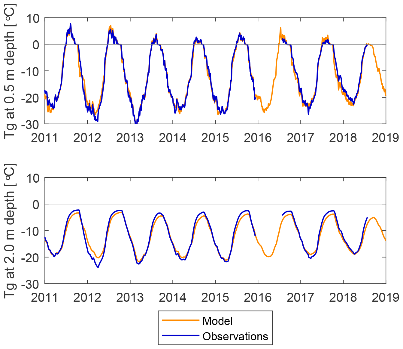
Figure A1 Observed and simulated ground temperatures T_g at 0.5 and 2.0 m depth in Aulavik Nationalpark, Banks Island.