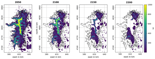
Projecting the evolution of the Northern Patagonian Icefield until the year 2200

The Northern Patagonian Icefield (NPI), Chile, is the second-largest ice mass in the Southern Hemisphere outside Antarctica and a major remnant of the Patagonian ice sheet from the Last Glacial Period. It is located in the Southern Andes, which is among the world’s glacierized regions with the most negative specific mass balances. The NPI is a highly dynamic system, with high amounts of accumulation and ablation, and includes San Rafael Glacier, the tidewater calving glacier closest to the equator.

Using the ice-sheet model SICOPOLIS, we reproduce the dynamical state and observed changes of the NPI in the early 21st century and project its evolution until 2200. Calving is represented by prescribing an additional mass loss for ocean-terminating grid cells (San Rafael Glacier). A spin-up experiment generates an icefield comparable to conditions around the year 2000, which we then force with present-day and projected surface mass balance under climate scenarios SSP1-2.6 and SSP5-8.5.

In the committed mass loss run, the NPI loses 36 % of its current mass by 2200. Under climate change scenarios, mass loss accelerates from the mid-21st century and continues until 2200, despite assuming constant climate during the final century. The NPI exhibits a response time of approximately 100 years, highlighting the need for caution when interpreting current trends. By 2200, the remaining volume strongly depends on the emission pathway: between 25 % and 62 % under SSP1-2.6 and between 6 % and 19 % under SSP5-8.5. These results confirm that for Patagonia, as found elsewhere, every fraction of a degree of warming matters.

1 Introduction

Glaciers are shrinking all over the world and, under business-as-usual emission scenarios, many mountain ranges are projected to be largely deglacierized by the end of the 21st century (Marzeion et al., 2020; Rounce et al., 2023). In the Southern Andes, the specific mass balance of glaciers was estimated to be among the most negative worldwide (Zemp et al., 2019). Due to the large amount of ice in the Southern Andes, which is mostly stored in a few large icefields, the projected relative mass loss until the end of the century is moderate: the Glacier Model Intercomparison Experiment (GlacierMIP) (Marzeion et al., 2020) suggests losses between 21 % under RCP2.6 and 41 % under RCP8.5 with respect to the estimated glacier mass in 2015.

The global models that participated in GlacierMIP have reduced capacities to reproduce the complex dynamics of ice bodies like the Northern Patagonian Icefield (NPI) and the Southern Patagonian Icefield (SPI): when projecting the geometry change of the ice body, they rely on volume-area scaling or flowline models (Marzeion et al., 2020). Only two of the eleven models parameterize frontal ablation, which can make a very important contribution to the total ablation of the large calving glaciers of the Patagonian Andes (up to 91 %, Minowa et al., 2021).

To our knowledge, projections have been carried out for only two glaciers of the Southern Andes using higher-order flow models: San Rafael Glacier, the largest glacier of the NPI (Collao-Barrios et al., 2018), and the Mocho-Choshuenco ice cap in the Chilean Lake District (Scheiter et al., 2021). Collao-Barrios et al. (2018) used the finite-element ice-flow model Elmer/Ice to model the behaviour of San Rafael Glacier. Assuming a fixed glacier outline and neglecting elevation feedbacks for the surface mass balance (SMB), they project a committed mass loss of 33.7 Gt, which corresponds to 14 % of the estimated glacier mass of the year 2000. Scheiter et al. (2021) modelled the dynamics of the Mocho-Choshuenco ice cap using the SImulation COde for POLythermal Ice Sheets (SICOPOLIS). Temperature projections from 23 models of Phase 5 of the Coupled Model Intercomparison Project (CMIP5) (Taylor et al., 2012) and a temperature-dependent parameterization of the equilibrium line altitude (ELA) were used to project the future SMB of the ice cap. They projected a relative volume loss between 56 % (RCP2.6) and 97 % (RCP8.5) at the end of the 21st century. The actual and future SMB of the entire NPI was studied by Schaefer et al. (2013) and Bravo et al. (2021). Schaefer et al. (2013) used an SMB model that considers solid precipitation as accumulation and calculates surface ablation as a function of incoming solar radiation, albedo and temperature. The model is driven by statistically downscaled global climate datasets: NCEP/NCAR for the period 1975–2011 and ECHAM-5 A1B scenario for the future. They found a slightly negative SMB of the NPI with an increasing trend during the recent past (1975–2011). A decreasing trend of the SMB was projected for the second half of the 21st century due to an increase in surface ablation and a decrease in accumulation. The modelled SMB showed a significant correlation with the projected annual mean temperature over the model domain (see Sect. 3.2.2). Bravo et al. (2021) used dynamically downscaled outputs of the MPI-ESM-MR Earth system model obtained with the regional climate model RegCM4.6 at 10-km spatial resolution between 1976 and 2005 and for the RCP2.6 and RCP8.5 scenarios, between 2005 and 2050. These products were used directly to estimate snow accumulation and subsequently to feed an energy balance model to estimate the ablation and its changes over both Patagonian icefields. For the NPI they projected an insignificant decrease in the SMB during the first half of the 21st century (−0.01 m w.e. a⁻¹) under the RCP2.6 scenario and a slightly higher and significant decrease under the RCP8.5 scenario (−0.08 m w.e. a⁻¹).

Here we study the complex ice dynamics of the NPI using the SImulation COde for POLythermal Ice Sheets (SICOPOLIS) (SICOPOLIS Authors, 2025) to better understand its current changes and project its evolution until the year 2200. We realize a spin-up to generate an icefield similar to the state of the NPI in the year 2000. We calibrate key model parameters by comparing our simulations to remotely sensed observations of elevation change (2000–2014) (Braun et al., 2019) and surface velocity (Mouginot and Rignot, 2015; Friedl et al., 2021). We choose the best set of model parameters and continue the simulations into the future with a constant (current) SMB to obtain the committed mass loss. In a next step, we use the temperature dependence of the projected SMB by Schaefer et al. (2013) to generate SMB anomalies for the CMIP6 model mean temperature projection (mean of NPI grid cells) in the 21st century for the pathways SSP1-2.6 and SSP5-8.5 (corresponding to RCP2.6 and RCP8.5 in CMIP5). For the 22nd century, we generate SMB anomalies for the NPI without trend by arbitrarily choosing one year of the last decade of the 21st century using the corresponding (model mean) temperature projection. Using these SMB anomalies, we project the evolution of the NPI until 2200 under the different scenarios of climate change.

2 Study site

The NPI with an area of 3700 km² (Meier et al., 2018) is the second largest ice mass in the Southern Hemisphere outside of Antarctica. Similar to the European Alps, it is located at moderate latitudes (Fig. 1), which are considerably lower than in other glaciated regions with maritime influence (Alaska or Northern Europe).

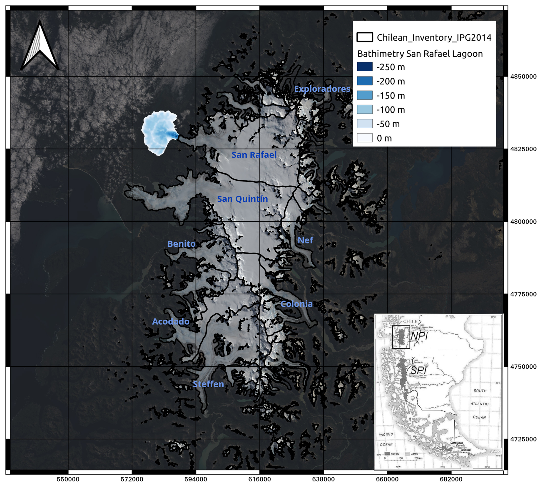
Figure 1 Main figure: NPI and some of its most important glacier catchments and bathymetry of San Rafael Lagoon; glacier outlines from Barcaza et al. (2017) that are consistent with Randolph Glacier Inventories version 6.0 & 7.0 for the main catchments of the NPI; bathymetry data from Koppes et al. (2011); coordinates are UTM 18S, superposed grid cells are 20×20 km; background satellite image is a true-color composite of Landsat image acquired on 12 March 2016; Inset: location of the NPI in southern South America.

San Rafael Glacier (the only tidewater calving glacier of the NPI) is the tidewater calving glacier closest to the equator. For the period 2000–2019 Minowa et al. (2021) found a mean annual frontal ablation of 0.99±0.29 Gt a⁻¹ for San Rafael Glacier, which corresponds to 36 % of its total ablation. Fürst et al. (2024) found a slightly higher frontal ablation value for San Rafael Glacier of 1.26±0.21 Gt a⁻¹ for the beginning of the 21st century (using glacier geometries of the year 2000 and ice velocities from Mouginot and Rignot, 2015). Several other glaciers of the NPI calve into rather small pro-glacial lakes, and their frontal ablation accounts for less than 20 % of their total ablation (Minowa et al., 2021). Measurements were performed over the outlet tongues of the glaciers Colonia and Nef using airborne radar systems, and ice thicknesses of over 700 m were detected (Blindow et al., 2012a). On the plateau area of the NPI, ice thickness was inferred from gravimetry measurements reaching values of up to 1400 m (Millan et al., 2019). Recently, the ice thickness of the NPI was modelled using a mass conservation approach, which considered all available ice thickness measurements over the NPI (Fürst et al., 2024).

3 Methods

3.1 Ice-flow model

The three-dimensional, dynamic and thermodynamic model SICOPOLIS was originally created in a version for the Greenland ice sheet (Greve, 1997a, b). Since then, the model has been developed continuously and applied to problems of past, present and future glaciation of Greenland, Antarctica, the entire Northern Hemisphere, the polar ice caps of the planet Mars, and other places, resulting in more than 150 publications in the peer-reviewed literature (https://www.sicopolis.net, last access: 5 June 2025).

Mainly developed for ice sheets, smaller ice bodies have also been modelled with SICOPOLIS, namely the Austfonna ice cap (Dunse et al., 2011) and the Mocho-Choshuenco ice cap (Scheiter et al., 2021). For this study, we apply SICOPOLIS v25 (SICOPOLIS Authors, 2025) to the NPI, using a polar stereographic projection with the WGS84 reference ellipsoid, standard parallel 47° S and central meridian 75° W (same as for UTM 18S). The stereographic plane is spanned by the Cartesian coordinates x (easting) and y (northing), discretized by a regular (structured) grid with resolution Δx=0.9 km. In the vertical, we use a terrain-following coordinate ζ (equal to 1 at the ice surface and 0 at the ice base; “sigma transformation”) instead of the physical coordinate z, with 81 layers in the ice domain, concentrating towards the base.

For the ice rheology, we use the regularized Glen flow law in the form of Greve and Blatter (2009, Sect. 4.3.2). The dynamics of grounded ice is modelled by the hybrid shallow-ice–shelfy-stream formulation. In this mode, the 3D velocity field is computed by the Shallow Ice Approximation if the local slip ratio (basal to surface velocity) is less than a threshold value, chosen as 50 %. Otherwise, the velocity field is computed as a weighted average between the Shallow Ice Approximation and the shelfy-stream approximation (Bernales et al., 2017; Greve et al., 2020). Ice thermodynamics is modelled by the one-layer melting-CTS enthalpy scheme (CTS: cold-temperate transition surface; Blatter and Greve (2015); Greve and Blatter, 2016). The temperature-dependent rate factor for cold ice is computed following Cuffey and Paterson (2010) (Sect. 3.4.6), and the water-content-dependent rate factor for temperate ice following Lliboutry and Duval (1985).

The ice surface is assumed to be traction-free. Basal sliding at the glacier bed is parameterized by a linear sliding law, in which the slip velocity v_b is proportional to the basal shear stress τ_b:

$$\begin{array}{}\text{(1)}& v_{\mathrm{b}}=-C_{\mathrm{b}}{\mathit{\tau }}_{\mathrm{b}}.\end{array}$$

The sliding function C_b is assumed to depend on the basal temperature relative to pressure melting T_b and the thickness of the basal water layer H_w:

$$\begin{array}{}\text{(2)}& C_{\mathrm{b}}=C_{\mathrm{b}}^{\mathrm{0}}\exp \left({\displaystyle \frac{T_{\mathrm{b}}}{\mathit{\gamma }}}\right)\left[\mathrm{1}+C_{\mathrm{w}}(\mathrm{1}-\exp \left(-{\displaystyle \frac{H_{\mathrm{w}}}{H_{\mathrm{w}}^{\mathrm{0}}}}\right)\right],\end{array}$$

where H_w is computed by a steady-state routing scheme for subglacial water that receives its input from the basal melting rate under grounded ice (Le Brocq et al., 2006, 2009), $C_{\mathrm{b}}^{\mathrm{0}}$ is the sliding coefficient, C_w the coefficient for water-layer-enhanced sliding, γ the sub-melt-sliding parameter and $H_{\mathrm{w}}^{\mathrm{0}}$ the threshold water-layer thickness. We use C_w=99, γ=10 K and $H_{\mathrm{w}}^{\mathrm{0}}=\mathrm{1}$ cm. In Fig. A1 we show how the sliding function C_b varies with the water-layer thickness H_w at several basal temperatures using $C_{\mathrm{b}}^{\mathrm{0}}=\mathrm{2}\times {\mathrm{10}}^{-\mathrm{4}}$ m a⁻¹ Pa⁻¹.

Due to the rather small size of the icefield and short simulations periods, we ignore glacial isostatic adjustment and assume a rigid bed instead. In addition, we ignore the thermal inertia of the lithosphere and apply the geothermal heat flux, chosen as q_geo=65 mW m⁻², directly at the base of the ice cap (based on Hamza and Muñoz, 1996). Sensitivity tests using q_geo=30 and 100 mW m⁻² were performed for the “best set” of model parameters (see below) leading to indistinguishable results during the calibration phase (see Sect. 4.1). Further model parameters are listed in Table A1.

We implemented a new calving condition that adds an additional mass loss at grid cells in contact with the ocean. In the NPI, this occurs only at the front of the San Rafael Glacier. We chose a constant additional mass loss per grid cell in a way that the overall modelled loss by calving fits the current observed calving flux for this glacier (Minowa et al., 2021). At the spatial model resolution of 900 m, the front of San Rafael is represented by two grid cells. At this model resolution applying a constant additional mass loss of 1000 m i.e. a⁻¹ gives a maximum calving flux of 1.46 Gt a⁻¹. The “real” calving fluxes are often lower then this value since sometimes there is not enough ice to calve of ( no negative ice thickness is allowed). Since this approach turned out to generate satisfactory results for the front position of San Rafael Glacier, we did not investigate more sophisticated “calving laws”. Since the amount of frontal ablation at lake-terminating glaciers is small in comparison with other mass-loss terms (22 % of the total frontal ablation (Fürst et al., 2024), which accounts for around 18 % of the total ablation (Minowa et al., 2021)), and future changes are very difficult to predict, we decided to neglect calving of lake-terminating glaciers.

3.2 Data

3.2.1 Bed topography

Consistent bed topography data is one of the most crucial inputs for ice-flow modeling. For our study, the basal topography map for the ice-covered parts of the NPI was generated using a mass-conservation approach (Fürst et al., 2024). The approach assimilated available thickness measurements and relied on glacier geometry (RGI Consortium, 2017; Farr and Kobrick, 2000), 1975–2011 climatic mass balance (Schaefer et al., 2013) and 2004 velocity information (Mouginot and Rignot, 2015). For NPI thickness observations, two regional airborne gravimetry campaigns from 2012 and 2016 (Gourlet et al., 2016; Millan et al., 2019) were considered, as well as a terrestrial gravimetry from 1985 (Casassa, 1987). Radar measurements of different spatial resolution were used on San Rafael, San Quintin, Soler, Nef and Colonia glaciers (Rivera, 2012; Blindow et al., 2012a; Pȩtlicki et al., 2023). For San Rafael Lagoon, bathymetry information was available from a 2006 sonic survey (Koppes et al., 2010). According to the generated bed topography map, 78 % of the NPI frontal ablation is channelized through San Rafael Glacier (Fürst et al., 2024), which justifies our approach to focus on this glacier when implementing the frontal ablation scheme in SICOPOLIS (see above).

3.2.2 Present and future surface mass balance

The surface mass balance (SMB) used to drive our simulations was derived from an extensive study of the interaction of NPI with its local climate (Schaefer et al., 2013). In this study, a regional climate model was run on a 5 km grid forced by reanalysis data. The climate data were further statistically downscaled to feed an SMB model of intermediate complexity in which surface melt was determined by a semi-empirical formula, which depends linearly on the atmospheric surface temperature but also on the net shortwave radiation (Oerlemans, 2001). This approach reproduced the expected pattern in which the glacier tongues on the Eastern side receive much more solar radiation as compared to the rest of the icefield (Fig. 8 in Schaefer et al., 2013). The model parameters were adjusted to reproduce the observed mass changes from geodetic studies and direct observations such as ablation stakes at Nef and San Rafael glaciers and two shallow firn cores taken in the accumulation area of San Rafael and Colonia glaciers. To realize projections, the physical downscaling of the reanalysis data was statistically analyzed and a statistical downscaling was applied to the projections of the ECHAM5 model (A1B) scenario (Schaefer et al., 2013). The resulting annual mean SMB of the NPI shows a strong correlation with the projected temperature anomaly (Fig. 2, left panel). In this contribution, we make use of this linear dependency and construct projected SMB anomalies under current climate change scenarios using projected temperature anomalies in the 21st century (Fig. 2, right panel). For the projected temperature anomaly times series, we use the mean value of 33 models of Phase 6 of the Coupled Model Intercomparison Project (CMIP6) (O'Neill et al., 2016), which are listed in detail in the Appendix (Table A2). To quantify the uncertainty of the temperature projections, we calculated the standard deviations between the temperature anomalies projected by the climate models and generated SMB anomalies corresponding to model mean temperature anomaly projections plus/minus one standard deviation (discontinuous lines, Fig. 2 right panel). It is important to note that these standard deviations are calculated on the temperature anomalies that were calculated with respect to the reference period 2000–2020 and not on the absolute temperatures. Since in Schaefer et al. (2013) the future SMB was modelled on fixed terrain elevation, we adjusted the SMB (and surface temperature) to modelled ice surface elevation in SICOPOLIS using fixed elevation gradients of 0.619 K/(100 m) and 1.13 m w.e./(100 m), which were obtained from SMB simulations of Schaefer et al. (2013). To be able to observe the adjustment of the NPI to the strongly transient climate in the 21st century, for the 22nd century, we used temperature anomalies without a trend by randomly picking a year of the last ten years of the 21st century and using the associated temperature and SMB anomalies.

Figure 2 Left: Relationship of NPI averaged surface mass balance and temperature anomalies for the 21st century (from Schaefer et al., 2013). Right: Temperature anomalies over the NPI as projected by the ECHAM5-Model (A1B scenario, green lines) (Roeckner et al., 2003) and the mean (red and blue solid lines) ± one standard deviation (discontinuous lines) of 33 CMIP6 models (Table A2). The selected reference period for the anomalies is 2000–2015.

3.2.3 Ice speed

Ice speed observations of the NPI were taken from remote sensing studies by Mouginot and Rignot (2015) for the year 2004, and by Friedl et al. (2021) for each of the years 2014–2020. They were used to calibrate the sliding coefficient $C_{\mathrm{b}}^{\mathrm{0}}$ (Eq. 2) and the enhancement factor E of the flow law. The general pattern of the ice motion did not vary too much over our calibration period 2000–2020.

3.2.4 Elevation change

Observed elevation changes for the early 21st century are available from geodetic surveys (e.g. Braun et al., 2019). The capacity of our model to reproduce these observed elevation changes is a good indicator for the reliability of our projections for the rest of the 21st and 22nd century. However, currently observed changes might be caused by changes in climate and ice dynamics in the past. Additionally, it is impossible to exactly generate the state of the NPI in 2000 during the spin-up (see below). Therefore, we do not expect to be able to reproduce exactly the observed elevation changes. We used the observed elevation changes generated by Braun et al. (2019) for 2000–2014 to optimize model performance during the calibration period (2000–2020).

3.3 Modelling workflow

In order to generate an icefield with similar characteristics as the NPI around 2000, we realized spin-up runs with a constant SMB. Using the 1975–2011 mean SMB generated by Schaefer et al. (2013), the resulting icefield has a much lower volume compared to the observed one (not shown). This indicates that the NPI in 2000 probably was not in equilibrium with the current climate which is in line with the mean elevation change of −0.88 m a⁻¹ during 2000–2014 by Braun et al. (2019) (see e.g. Fig. 5). We therefore realize the spin-up with a more positive, constant SMB, which, according to the linear relationship between temperature and SMB indicated in Fig. 2, corresponds to a colder climate. When using a constant SMB that corresponds to a one degree colder climate, after approximately 500 years a steady state is reached that has a similar overall ice volume (maximum 3 % of difference, Table 1), surface elevations (RMSD∼88 m) and surface velocities (RMSD∼351 m a⁻¹). Separate spin-ups for the nine different combinations of model parameters indicated in Table 1 were realized in order to avoid model drift during the calibration period.

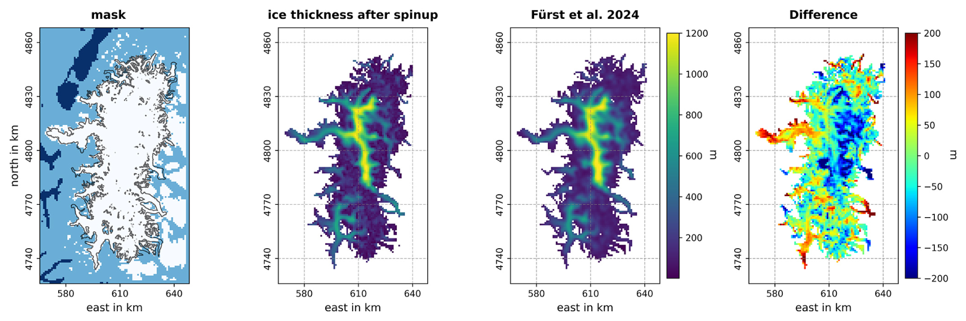
Figure 3 Comparison of the NPI state after the spin-up to observations; left: modelled mask (white: ice, light blue: land, dark blue: ocean) and observed year 2000 outlines (black contour), middle: modelled ice thickness after the spin-up clipped to the year 2000 outlines for a better comparison, right: modelled ice thickness for the year 2000 by Fürst et al. (2024).

Figure 4 Comparison of the NPI surface velocities after the spin-up to observations; left: modelled velocities after the spin-up clipped to the year 2000 outlines; right: observed surface velocities by Mouginot and Rignot (2015), which are centred around the year 2004. Observed year 2000 glacier outlines are shown in grey

In the next step, the icefield generated in the spin-up is forced with temperature anomalies for the years 2000–2020 (we chose to take them from SSP1-2.6, which is identical to SSP5-8.5 in the first 15 years), and the evolution of the icefield during this period is compared to observations of elevation change (Braun et al., 2019) and ice motion (Mouginot and Rignot, 2015; Friedl et al., 2021). The empirical model parameters ($C_{\mathrm{b}}^{\mathrm{0}}$, the enhancement factor E) were varied, and a comparison of the simulation results with observations was performed (see Table 1). Additional sensitivity tests were realized with the model parameters q_geo and $H_{\mathrm{w}}^{\mathrm{0}}$. The results showed very low sensitivity on the variation of q_geo and in the SSP5-8.5 run the 2200 volume varied by approx ±2 % when using double or half $H_{\mathrm{w}}^{\mathrm{0}}$ respectively.

Using the best empirical model parameter set (defined below), the simulations were driven by the different 2000–2100 climate change scenarios, which were continued until 2200 using temperature anomalies from 2090–2099 (see above) for the 22nd century. To obtain an estimate of the committed mass loss, a simulation was run with a constant SMB (1975–2011 mean, Schaefer et al., 2013).

4 Results

4.1 Model calibration

In order to obtain model results that are most similar to the observations in the validation period 2000–2020, we systematically varied the enhancement factor E of the flow law and the empirical constant $C_{\mathrm{b}}^{\mathrm{0}}$ of the basal sliding coefficient (Eq. 2). Table 1 summarizes the performance of the different model calibration runs.

Table 1 Results of the calibration runs with varied enhancement factor E and basal sliding coefficient $C_{\mathrm{b}}^{\mathrm{0}}$. “Bias” and “RMSD” refer to the linear and quadratic mean, respectively, of the differences between the model results and the observations (“bias” is therefore positive if the model results are higher than the observations). Selected parameter set and associated metrics are marked in boldface.

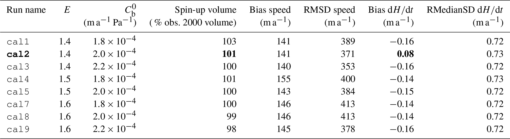
We report the root median square deviation (RMedianSD) rather than the root mean square deviation (RMSD), as the model cannot reproduce the exact calving-front geometry of San Rafael Glacier. This limitation leads to localized, large positive and negative differences between modelled and observed elevation changes that substantially influence the RMSD, whereas the RMedainSD provides a more robust measure of the typical model misfit.

We argue that the most important quantity for calibration is the Bias of the elevation change (which is proportional to the overall ice loss). Therefore, we chose the parameters used in the run cal2 for the projections. In Fig. 5, we visualize the modelled and observed elevation change using these model parameters.

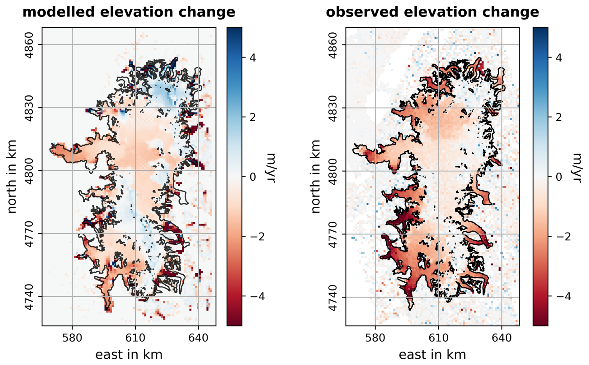
Figure 5 Modelled (left) and observed (right) elevation changes for 2000–2014.

4.2 Committed mass change and projections under climate change scenarios

Once having determined the “best parameter set”, we realize future simulations starting from the state generated by the spin-up run (Figs. 3, 4). For the committed mass loss run, we use a constant SMB that corresponds to the 1975–2011 mean modelled one by Schaefer et al. (2013). For the climate change scenarios, we use SMB projections derived from temperature projections of the SSP1-2.6 and SSP5-8.5 scenarios of 33 CMIP6 models (see Table A2 and Sect. 3.2.2). The projected ice volume is presented in Fig. 6 (relative changes in Table A3).

Figure 6 Simulated evolution of the total ice volume of the NPI during the 21st and 22nd centuries under a constant current climate (black dashed), the SSP1-2.6 scenario (blue lines) and the SSP5-8.5 scenario (red lines). The continuous lines are based on global circulation model mean temperature anomalies, and the dashed lines on mean ± one standard deviation.

The committed mass loss run projects more than 35 % of the initial (year 2000) mass to be lost by 2200. In the SSP1-2.6 scenario more than 55 % of the icefield's mass is projected to be lost by 2200 and in the SSP5-8.5 scenario only 10 % of year 2000 ice mass is projected to remain. In Figs. 7 and 8.

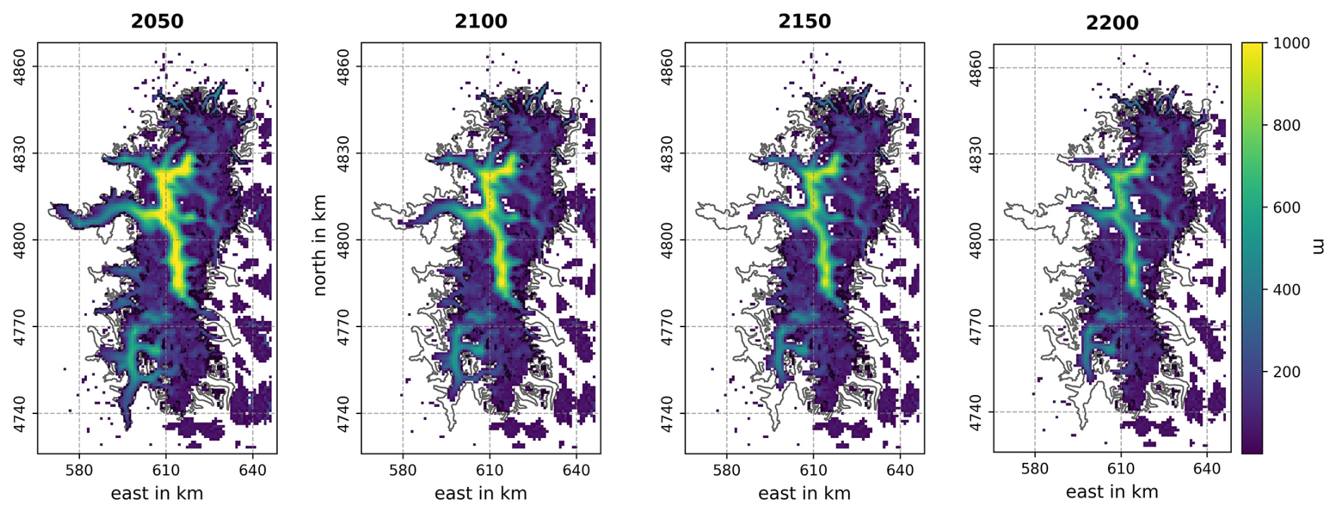
Figure 7 Simulated ice thickness of the NPI in the 21st and 22nd centuries under the SSP1-2.6 scenario. Year 2000 icefield outlines are shown for comparison.

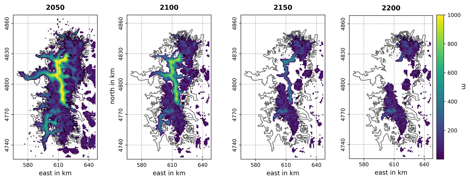
Figure 8 Simulated ice thickness of the NPI in the 21st and 22nd centuries under the SSP5-8.5 scenario. Year 2000 icefield outlines are shown for comparison.

we show the evolution of the ice thickness distribution under the climate change scenarios SSP1-2.6 and SSP5-8.5. For SSP1-2.6, all glaciers retreat and current glacier tongues disappear by the end of the 22nd century (details on relative area losses are indicated in Table A4). The largest glaciers of the NPI, San Rafael and San Quintín glaciers, maintain small tongues and in the plateau between San Rafael Glacier and Colonia Glacier ice thickness by 2200 is still over 600 m (Fig. 7). By contrast, for SSP5-8.5, the ice thickness distribution in the year 2100 is similar to the final one in the moderate scenario and the icefield splits up into two major ice bodies after 2150. Maximum ice thickness of these ice bodies by 2200 is projected to be below 400 m (Fig. 8). Information on SMB and ice speed of the projected ice bodies in the two climate change scenarios are presented in Figs. A2, A3.

5 Discussion

Our results provide the first projections for the evolution of the NPI as a whole using a three-dimensional ice-flow model. Important differences in comparison to previous projections for or on the NPI are:

• the implementation of a calving law, which lets the ice front freely evolve,

• the simulations were run until 2200, which allows adjustment of the icefield adjust to the strong expected climate trends during the 21st century,

• the use of SMB data that are consistent with direct observations.

In Fig. 9, we compare our ice volume projections to other studies. The only study that provides projections for the NPI is Aguayo et al. (2024), who used the Open Global Glacier Model (OGGM) (Maussion et al., 2019). They project much higher mass loss during the 21st century than our study, and also compared to the projections for the Southern Andes by the Glacier Model Intercomparison Project (Marzeion et al., 2020). We think the reason for this is that calving is not implemented in the OGGM version used by Aguayo et al. (2024). Since the model is calibrated against geodetic mass balances (which include calving losses), the temperature sensitivity parameter necessary to reproduce the negative mass balance of the NPI during their calibration period (2000–2020) is probably chosen too high, which explains the high mass losses projected for the 21st century. Another reason for the disagreement could be the different surface mass balance models: here we realy Schaefer et al. (2013), who used a semi-empirical energy balance to model glacier melt, whilst the OGGM version used by Aguayo et al. (2024) uses a temperature index model. In summary, we think that Aguayo et al. (2024) probably present reliable projections for glacier regions in Patagonia with smaller glaciers, which do not experience important mass losses by calving, their results for the large icefields of Patagonia (NPI, SPI, Cordillera Darwin), where frontal ablation contributes up to 48 % to total ablation (Minowa et al., 2019), should be interpreted with much care.

Figure 9 Projection of relative glacier volume change in the Southern Andes throughout the 21st century, relative to 2020, from different studies.

Our volume evolution projections for NPI predict higher relative mass loss than the Glacier Model Intercomparison Experiment for the entire Southern Andes (Marzeion et al., 2020). Although the NPI is one of the most important ice bodies in the Southern Andes, the SPI holds approximately 3.5 times the ice volume of the NPI (Fürst et al., 2024). The projection of this huge ice body should dominate the projections of the ice volume of the Southern Andes. The more moderate projected mass losses obtained in Marzeion et al. (2020) compared to Aguayo et al. (2024) are probably due to the implementation of calving losses in some of the global glacier models (Huss and Hock, 2015) and the use of direct SMB observations (instead of geodetic) for model calibration.

The evolution of the ice volume of the entire NPI in our committed mass loss simulation is showing higher relative mass loss rates compared to the results of Collao-Barrios et al. (2018) for San Rafael Glacier. One explanation could be that Collao-Barrios et al. (2018) used fixed glacier outlines, which did allow the glacier to retreat during their simulations. They also used a different bed geometry, mainly based on airborn gravimetry measurements, which shows shallower ice depths and consequently lower losses due to calving at the front of San Rafael Glacier.

Comparing our results to the projections of Scheiter et al. (2021) for the Mocho-Choshuenco ice cap, also located in the Wet Andes, their projected relative ice volume losses by the end of the century of 56±16 % for RCP2.6 and 97±2 % for RCP8.5 are much higher. This is in line with the results of global studies, where glacier regions with smaller glaciations experience higher percentage losses (see, e.g., Marzeion et al., 2020). As a consequence of this the relative ice volume losses should be significantly higher for the Dry Andes as for the Wet Andes. However, this distinction has not been captured well by global studies to date, as they typically group the highly contrasting Dry Andes and Wet Andes regions into a single category referred to as the “Southern Andes” (RGI Consortium, 2017).

Another interesting result of our study is that important glacier changes will continue during the 22nd century even under a constant late-21st-century climate (no further warming trend beyond 2100). We can compare this result to the theoretical formula for the glacier response time t_r (Cuffey and Paterson, 2010),

$$\begin{array}{}\text{(3)}& t_{\mathrm{r}}={\displaystyle \frac{H_{\max }}{a_{\mathrm{0}}}},\end{array}$$

where H_max is the maximum ice thickness and a₀ the ablation rate at the glacier tongue. From our input data, we find ${\stackrel{\mathrm{‾}}{a}}_{\mathrm{0}}=\mathrm{15.6}$ m i.e. a⁻¹, where we took an average over modelled ablation values at the tongues of the 17 most important glaciers of the NPI (Schaefer et al., 2013), and H_max=1440 m (Fürst et al., 2024), which results in t_r=92.3 a. This value is in good agreement with the continuing changes observed in our simulation under a constant climate during the 22nd century. A similar value was found by (Zekollari et al., 2025) for the Southern Andes Glacier region. This result indicates that the interpretation of observed mass changes (and their direct association with changes in climate, Noël et al., 2025) should be realized with caution since the observed mass changes may be influenced by climate changes that occurred in a time span of nearly 100 years.

This result also leads us to the main caveat of our study. The validation period is shorter than the expected response time. In future studies, longer calibration periods should be used to improve confidence in the results. Simulations since the Little Ice Age for which different glacier outline products are available (Glasser et al., 2011; Meier et al., 2018) are desirable. The problem of such simulations is the large uncertainty of the initial glacier state with respect to ice elevations and surface velocities. As a main contributor to ice volume changes in the Wet Andes (and the Southern Andes), a similar modelling effort should be realized for the SPI. Due to the much higher relative mass loss by frontal ablation there (48 %, Minowa et al., 2021), probably more sophisticated parameterizations of calving losses will have to be used in the ice-flow model.

6 Conclusions

In this contribution, we realize projections for the NPI under different climate change scenarios using a state-of-the-art ice-flow model including a simple implementation of frontal ablation for the tidewater glacier San Rafael. Our most important conclusions are as follows:

• large area, volume and morphological changes are projected until the year 2200 with important differences depending on the climate change scenario (56 % of ice loss in SSP1-2.6 and 90 % in SSP5-8.5),

• the NPI has a response time of approximately 100 years, which should be taken into account when interpreting current changes,

• future studies should consider larger time spans for model calibration and focus on the largest ice body of the Southern Andes, the Southern Patagonia Icefield.

Appendix A

Figure A1 Dependence of the basal sliding function C_b on the basal water-layer thickness H_w at different basal temperatures $T_{\mathrm{b}}^{\prime }$.

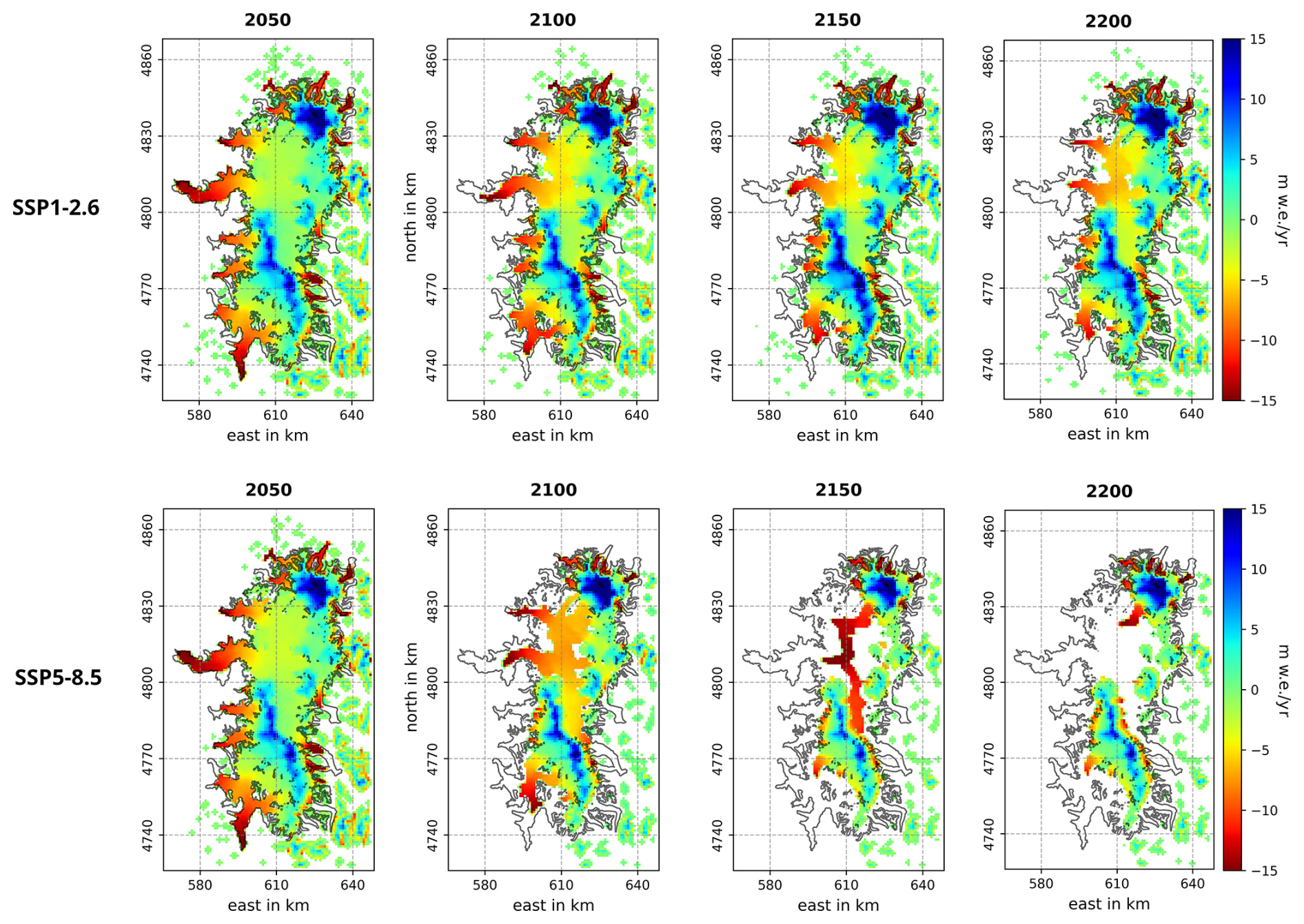
Figure A2 Surface mass balance of the projected ice bodies in the NPI area under two climate change scenarios.

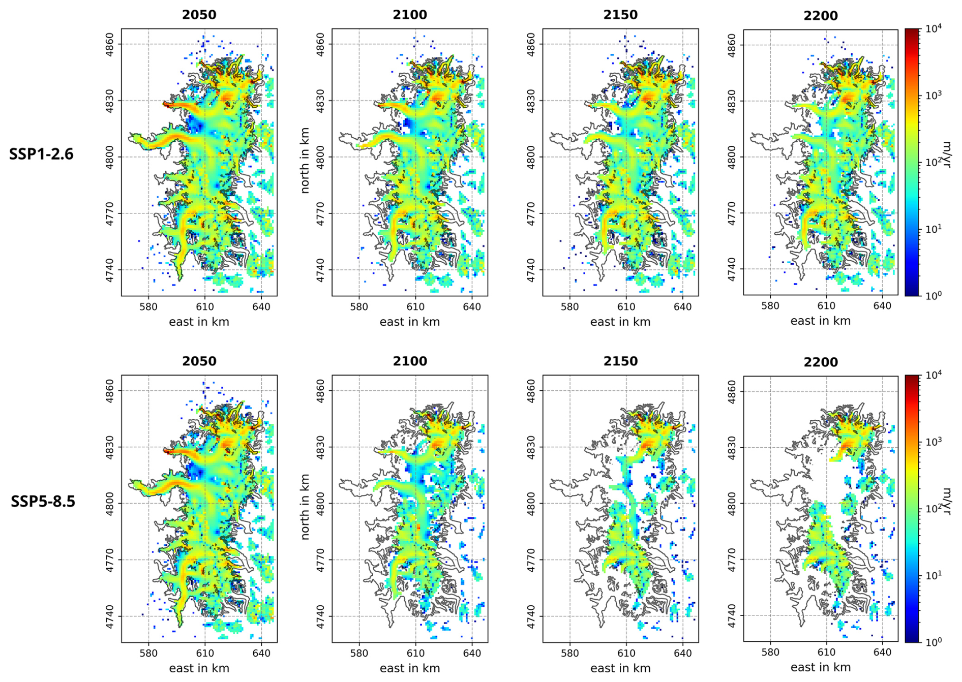
Figure A3 Ice speed of the projected ice bodies of the NPI area under two climate change scenarios.

Table A1 Physical parameters used for the simulations of this study.

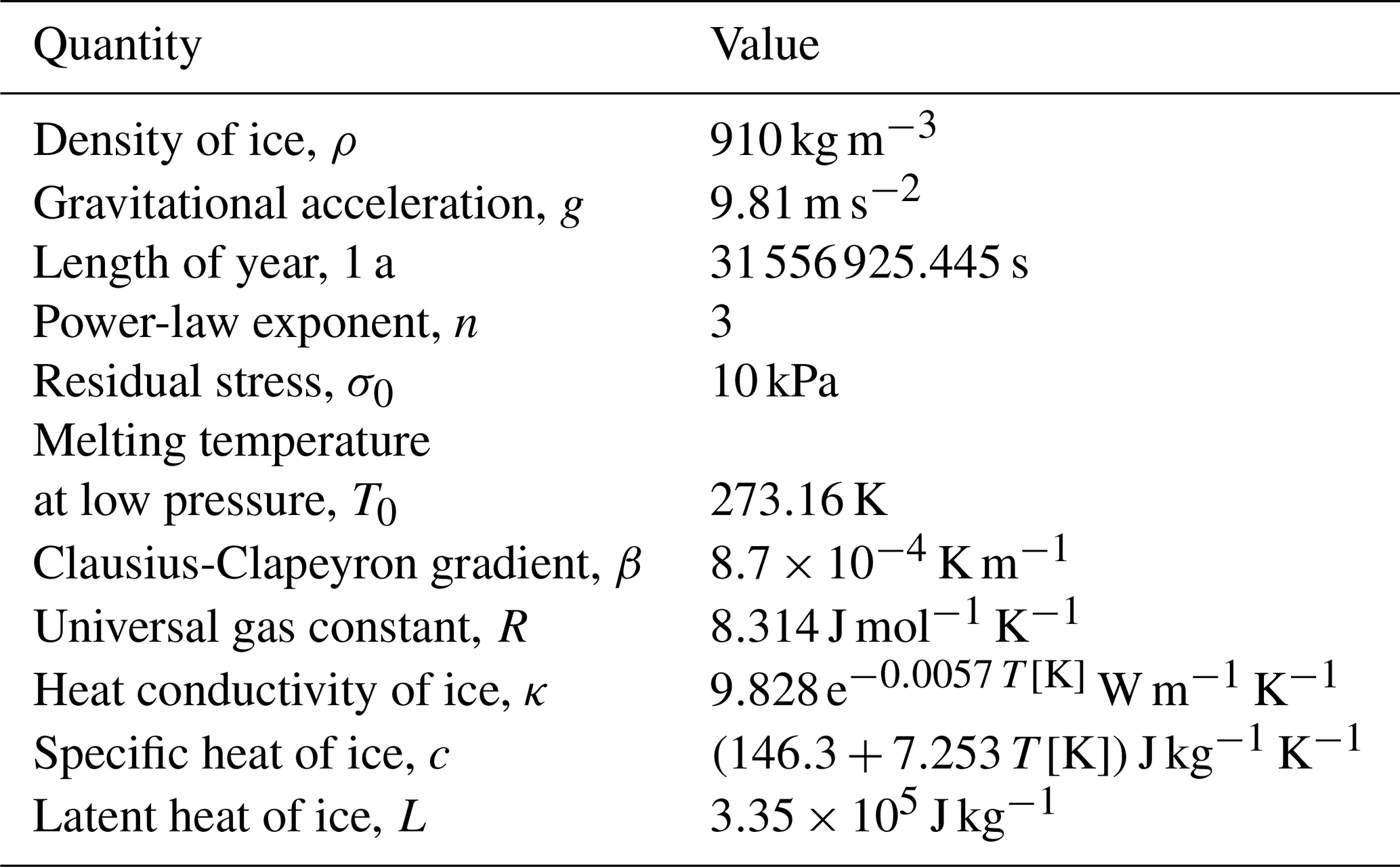
Table A2 Selected CMIP6 models and their projected 2090–2099 mean temperature anomaly (°C) with respect to years 2000–2015 for scenarios SSP1-2.6 and SSP5-8.5 and averaged over the NPI, and their spatial resolution.

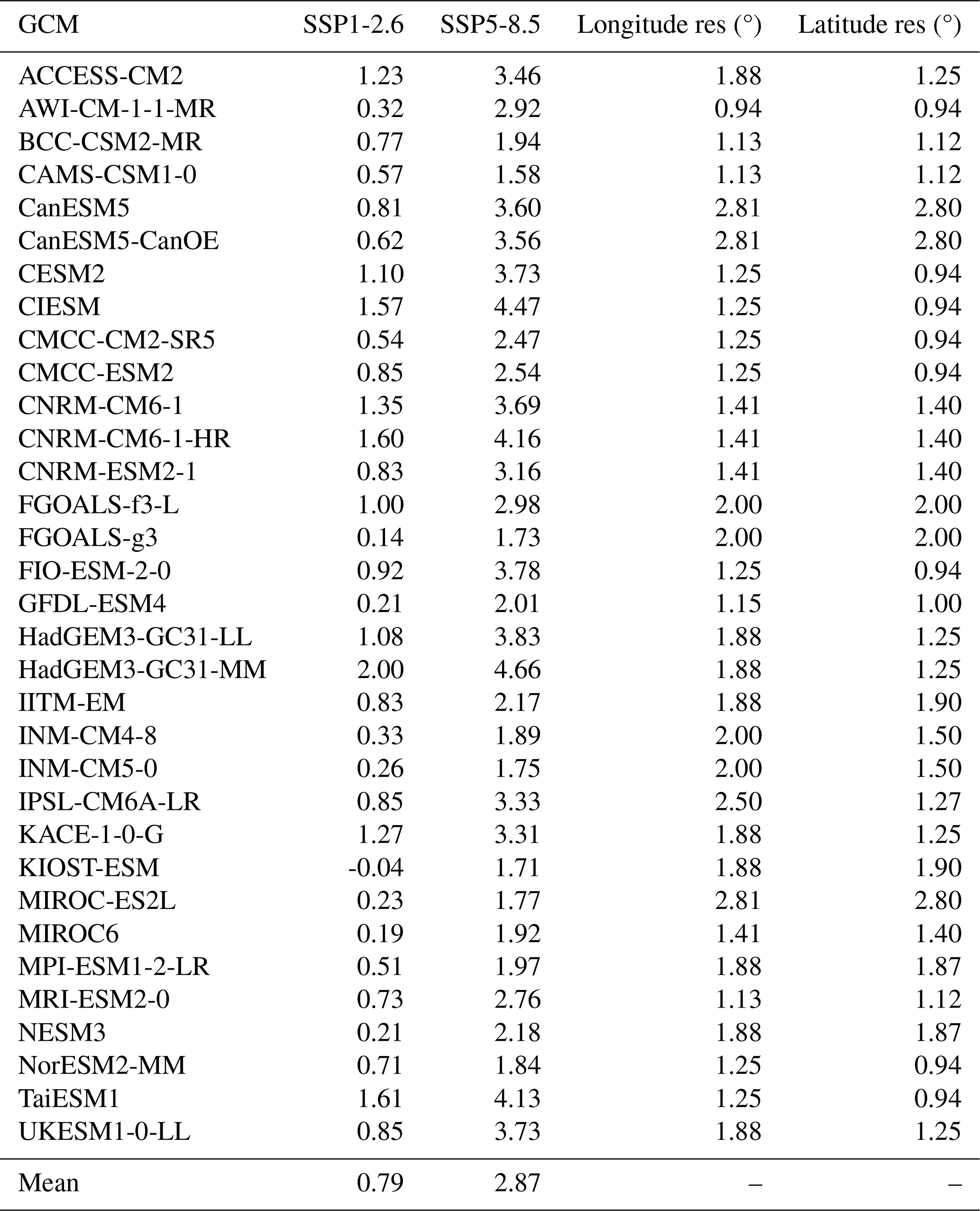
Table A3 Simulated ice volume as a percentage of the year 2000 volume.

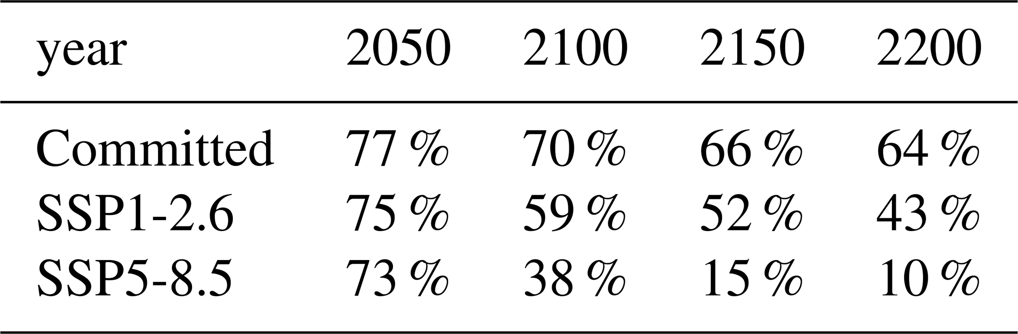
Table A4 Simulated icefield area as a percentage of the year 2000 area.