Evolution of the Antarctic Ice Sheet from 2000–2300 and beyond: model sensitivity and uncertainty analysis using MPAS-Albany Land Ice

We present a description of the Antarctic Ice Sheet model configuration submitted to the ISMIP6-Antarctica-2300 experiment using the MPAS-Albany Land Ice model, along with three new sets of simulations: (1) a set of extended simulations to 2500 for three forced experiments and to 2775 for the control experiment; (2) a sensitivity analysis of our model configuration to parameters controlling basal sliding and sub-shelf melt, and to model structural choices including the choice of the energy and stress balances; and (3) a 72-member ensemble run on graphics processing units (GPUs) and analysis of variance to determine the primary sources of uncertainty in our ice-sheet model projections. Our extended simulations predict rapid retreat beginning after 2300 for SSP1-2.6 forcing and after 2500 for present-day (control) forcing, primarily in the Amundsen Sea Embayment. We find that varying the sub-shelf melt parameter between the 5th to 95th percentile values for a mean-Antarctic calibration target results in an up to $\sim \pm$40 % change in sea-level contribution relative to our baseline simulations that used the median value. Using a linear basal sliding law reduces sea-level contribution by 51 %–73 % relative to our baseline nonlinear sliding law with an exponent of $\mathrm{1}/\mathrm{5}$. When using basal sliding law exponents of $\mathrm{1}/\mathrm{3}$ and $\mathrm{1}/\mathrm{10}$, the overall difference from our baseline simulations at 2300 is on the order of 10 %. The Amundsen Sea Embayment region displays a strongly non-linear dependence of mass loss on the sliding law exponent, with no discernible relationship between the sliding law exponent and the mass loss by 2300, while the sectors feeding the Ross and Filchner-Ronne ice shelves exhibit more mass loss with a more-plastic sliding law. Our model fidelity sensitivity experiments reveal a 9 %–31 % increase in sea-level contribution when using a depth-integrated stress balance approximation relative to our three-dimensional solver, while using a fixed-in-time temperature field increases sea-level contribution by 14 %–88 % relative to two thermomechanically coupled configurations. Our 72-member ensemble and analysis of variance show that the uncertainty in long-term projections is dominated by the choice of Earth system model forcing and the presence or absence of hydrofracture forcing, rather than uncertainty in sliding and sub-shelf melt parameters.

1 Introduction

The Antarctic Ice Sheet (AIS) contributed 14 ± 2 mm to global mean sea level between 1979 and 2017 (Rignot et al., 2019). Mass loss has been dominated by the Amundsen and Bellingshausen sea sectors, where incursions of warm and salty circumpolar deep water have driven increased ice-shelf melting, leading to dynamic thinning and increased discharge to the oceans (Shepherd et al., 2004; Pritchard et al., 2009; Jenkins et al., 2016; Smith et al., 2020). For glaciers with inland-deepening bed topography, the increase in melting raises the possibility of a positive feedback between ice discharge and grounding-line retreat, known as the Marine Ice Sheet Instability (MISI; Weertman, 1974; Schoof, 2007). MISI-style retreat may already be underway in the Amundsen Sea Embayment (ASE) and in particular at Thwaites and Pine Island glaciers (Joughin et al., 2014; Rignot et al., 2014; Favier et al., 2014). Onset of potentially unstable grounding-line retreat leads to multiple meters of sea-level rise in the coming centuries in some model simulations (e.g., Seroussi et al., 2024). Moreover, if the large Ross and Filchner-Ronne ice shelves experience a predicted switch from cold to warm ice-shelf cavity conditions, grounding-line retreat in some areas may be irreversible, even if the melt rates are reduced to cold-cavity levels (Hill et al., 2024). Thus, the AIS could dramatically retreat in the coming centuries, with little chance of re-advance in the absence of extreme ocean cooling.

However, ice sheet models disagree widely on the future behavior of the AIS for a given forcing scenario, leaving the AIS as the largest source of uncertainty in sea-level projections (Edwards et al., 2021). Seroussi et al. (2020), Edwards et al. (2021), and Payne et al. (2021) found that the sign of the overall sea-level contribution from the AIS by 2100 was uncertain, but Seroussi et al. (2020) noted that strong ocean warming in their scenarios, taken from CMIP5 simulations, only began in the last few decades of the 21st century. Therefore, the follow-on ISMIP6-Antarctica-2300 study (Seroussi et al., 2024) used a set of simulations from CMIP5 and CMIP6 models that were run out to 2300, as well as a number of constructed “repeat” forcings in which ocean and atmospheric conditions were sampled from the final decades of the 21st century to preserve natural variability in the forcing. The ISMIP6-Antarctica-2300 ensemble predicts a multi-meter range of possible sea-level contributions by 2300 for the high-emissions scenarios, with some ice-sheet models predicting nearly complete collapse of the West Antarctic Ice Sheet (WAIS) by 2300, and others predicting only modest retreat or slight mass gain. Even when using the same model codebase, the choices made by different modeling groups contributing to ISMIP6 lead to fundamentally different ice-sheet responses to forcing. It is perhaps not surprising, therefore, that Seroussi et al. (2024) found through a formal analysis of variance (ANOVA) that the choice of ice sheet model was the dominant source of uncertainty in projections of sea level by 2300. However, they were unable to determine the exact source (e.g., stress balance approximation, parameter values, numerical schemes, model resolution, initialization procedure, etc.) of this uncertainty, leaving an open question regarding the best approach to reducing uncertainty in model projections of sea-level change from Antarctica.

The sources of uncertainty in ice-sheet projections of sea-level change are myriad, and are rarely fully explored or quantified in modeling studies. While the emissions scenario – e.g., choice of Representative Concentration Pathway (RCP) or Shared Socioeconomic Pathway (SSP) – is certainly highly uncertain, many sources of uncertainty stem from choices and limitations in the ice-sheet models themselves. These can largely be separated into parametric, structural, and initial condition uncertainty. Structural uncertainty can be further subdivided into sources from model scope (i.e., which processes are represented), model form (i.e., which equations are used to represent these processes and how they are solved) and model fidelity (i.e., how well the choices represent the true physics). Initial condition uncertainty stems from the many different choices of input datasets, boundary conditions, calibration targets, and initialization procedures used by the various groups whose results are reported by Seroussi et al. (2024). By leaving almost all modeling choices aside from forcing scenarios up to the individual modeling groups, the ISMIP6-Antarctica-2300 experiment sampled parametric, structural, and initial condition uncertainty extremely widely, but also simultaneously and not systematically. Furthermore, as in the previous iteration of ISMIP6 (Seroussi et al., 2020), the analysis gave equal weight to all submissions regardless of their skill in reproducing historical ice-sheet behavior (Aschwanden et al., 2021), although historical accuracy was not a prerequisite for participating. Therefore, interpretation of the ISMIP6-Antarctica-2300 results in terms of individual sources of ice-sheet model uncertainty is quite difficult.

Efforts by individual modeling groups to understand the sources of uncertainty in their own simulations through sensitivity analysis represent a first step towards reconciling estimates of future Antarctic sea-level contribution. Previous studies using models that participated in ISMIP6 have found strong sensitivity to initialization procedures (van den Akker et al., 2025), treatment of sub-shelf melting (Lipscomb et al., 2021; O'Neill et al., 2025; Juarez-Martinez et al., 2024; Coulon et al., 2025), basal physics (Lipscomb et al., 2021; Zhao et al., 2025), and feedbacks between the ice sheet and the solid Earth (Han et al., 2025). Taken together, these previous studies highlight the importance of understanding the sensitivity of individual models to specific modeling choices, and they identify basal friction and sub-shelf melting as potentially two of the most impactful processes to examine.

In the spirit of better understanding the individual ice-sheet models that contributed to ISMIP6-Antarctica-2300, we explore the sensitivities of the MPAS-Albany Land Ice (MALI; Hoffman et al., 2018) AIS configuration to parameters controlling basal friction and sub-shelf melt. We additionally explore the sensitivity to two structural modeling choices that are widely sampled in the ISMIP6-Antarctica-2300 ensemble: the choice of stress-balance approximation and the treatment of the energy balance. Our simulations submitted to ISMIP6-Antarctica-2300 were the only ones to use a three-dimensional higher-order stress-balance solver, but we have recently implemented a Mono-Layer Higher-Order (MOLHO) solver that is more similar to the other higher-order solvers used in ISMIP6. The models participating in ISMIP6 use a wide range of thermal solvers, ranging from a spatially and temporally uniform temperature field to thermomechanically coupled enthalpy formulations, and thus differences in choices of energy balance solver could have a large impact on the spread of sea-level predictions in the ISMIP6 ensembles.

We begin with an overview of the MALI configuration that was used in ISMIP6-Antarctica-2300, followed by an investigation of the sources of uncertainty in the model configuration. We describe the MALI results of the ISMIP6-Antarctica-2300 experiments in more detail than was possible in Seroussi et al. (2024). We then select a subset of ISMIP6-Antarctica-2300 experiments to extend out to at least 2500 to explore further evolution of the ice sheet under a wide range of continued forcing. We follow this with a set of one-at-a-time sensitivity experiments that explore choices of parameter values controlling ice-shelf melting and basal sliding as well as choices of model fidelity controlling thermomechanical coupling and stress balance approximation. Finally, we use the understanding gained from the sensitivity experiments to construct a large ensemble of 72 simulations that explore combinations of parameter choices and forcing choices (i.e., Earth system model and ice-shelf hydrofracture) and perform an ANOVA to understand the sources of uncertainty in our single ice-sheet model. While our investigation excludes many possible sources of uncertainty in our model (e.g., subglacial hydrology, iceberg calving, evolving fabric, and glacial isostatic adjustment), we focus on processes that we expect to have a substantial impact on projections while also being feasible to explore in our model framework.

2 Model description, configuration, and experiments

2.1 The MPAS-Albany Land Ice model

MALI is a three-dimensional, higher-order, thermomechanically coupled numerical ice sheet model developed for Earth system modeling applications (Hoffman et al., 2018). It employs a dual mesh approach, in which a finite element code solves for ice velocity on a Delaunay triangulation mesh within the Albany multi-physics analysis package, while advection and other physics (e.g. submarine melting) are applied on the dual Voronoi tesselation. MALI typically uses the Blatter-Pattyn stress balance approximation (Blatter, 1995; Pattyn, 2003), which is a three-dimensional, first-order approximation of the Stokes equations. A Mono-Layer Higher-order (MOLHO) stress balance approximation has recently been added and is described in Appendix A. We use Nye's generalization of Glen's flow law for the constitutive relationship (Glen, 1955; Nye, 1957), with the temperature dependence of the flow parameter determined following Paterson and Budd (1982). Temperature- and enthalpy-based solvers are available for thermal evolution. The enthalpy-based solver differs from the temperature-based solver by additionally accounting for liquid water content of ice at the pressure-melting point. By default, thickness and tracers are advected by a first-order upwind scheme and we use first-order forward Euler time stepping. Second-, third-, and fourth-order flux-corrected transport schemes (Skamarock and Gassmann, 2011) and second- and third-order Strong Stability-Preserving Runge Kutta schemes (Durran, 2010) have also recently been added, but were not used in this study. We use adaptive time-stepping with a maximum time-step length determined by a user-defined fraction of the Courant-Friedrichs-Lewy (CFL) condition (Courant et al., 1928). We recently incorporated coupling to a sea-level model (Han et al., 2025), but these changes were not included here and thus the bed topography is held fixed in time for all simulations in this study.

2.2 Model initialization

We use a two-dimensional, 4–20 km variable resolution mesh, containing 385 379 cells and 5 terrain-following vertical layers with constant but nonuniform thickness fraction (i.e., a “sigma” vertical coordinate system). Cell spacing is determined both by observed surface velocity and by distance to the grounding line. The distance-based cell spacing linearly decreases from 4 km within 40 km of the grounding line to 20 km at a distance of ≥ 250 km from the grounding line. The velocity-based cell spacing is a linear function of log₁₀(u_obs), where u_obs is the observed surface velocity in meters per year, with 4 km spacing for log₁₀(u_obs)≥2.5 and 20 km spacing for log₁₀(u_obs)≤0.5. The minimum of these two cell spacing functions at each location is then assigned as the final cell spacing for the mesh. This cell spacing function ensures high resolution over the modern grounding line, ice streams, narrow outlet glaciers, ice shelves, and pinning points of sufficient size, while allowing for lower resolution in the modern-day slow-flowing ice-sheet interior regions to keep computational costs affordable. As MALI lacks an adaptive mesh refinement capability, this cell spacing is held fixed in time. In simulations predicting major grounding-line retreat in West Antarctica, the grounding line will eventually retreat into lower-resolution regions, leading to less accurate solutions later in the simulations. We discuss this limitation further in Sect. 4.5.

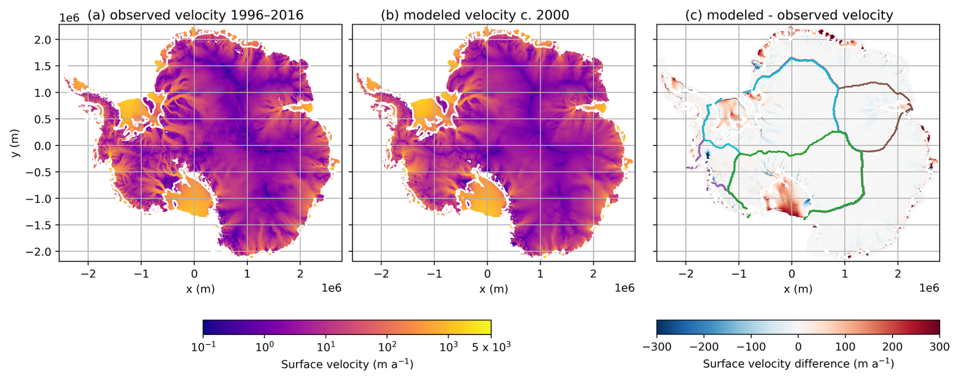
Figure 1 (a) Observed 1996–2016 composite surface velocities (Rignot et al., 2017). (b) MALI initial condition with a nominal date of 2000, following optimization to match observed 1996–2016 mean velocities in (a) and a ten-year relaxation simulation. (c) Difference between modeled and observed velocities. Colored contours represent the regions that we analyze throughout this study: purple – Amundsen Sea Embayment (ASE); cyan – Filchner-Ronne Ice Shelf (FRIS); green – Ross; brown – Amery. The grounding line is represented by white curves in all panels.

Our model initial condition is shown in Fig. 1. We use the adjoint optimization method constrained by partial differential equations described by Perego et al. (2014) and Hoffman et al. (2018) to simultaneously solve for basal traction and ice stiffness fields that minimize the misfit between the observed and modeled surface velocities while imposing regularization on the sliding coefficient. We use an ice temperature solution from a previous optimization on an 8–30 km mesh, which was then interpolated to our 4–20 km mesh and used as an input to the optimization for the basal traction and ice stiffness fields. The following data sources are used for the optimization:

• observed surface velocities: MEaSUREs 1996–2016 composite InSAR-Based Antarctica Ice Velocity Map, Version 2, 450 m resolution (Rignot et al., 2011; Mouginot et al., 2012; Rignot et al., 2017), interpolated to MALI mesh using conservative remapping

• bed topography and ice thickness: BedMachine Antarctica v2 (Morlighem et al., 2020), interpolated to MALI mesh using conservative remapping

• geothermal flux: Martos et al. (2017), interpolated to MALI mesh using barycentric interpolation.

• surface air temperature: Lenaerts et al. (2012), 1979–2010 mean, interpolated to MALI mesh using barycentric interpolation.

At the basal boundary, we use a power-law sliding relationship of the form ${\mathit{\tau }}_{\mathrm{b}}=\mathit{C}|{\mathit{u}}_{\mathrm{b}}{|}^{q-\mathrm{1}}{\mathit{u}}_{\mathrm{b}}$ (Weertman, 1957), where τ_b is the basal shear stress, C is the sliding coefficient solved, u_b is the basal sliding velocity, and q is a scalar plasticity parameter usually defined as $q=\mathrm{1}/m$, where m is a positive integer. For the optimization, we use the common assumption of $q=\mathrm{1}/\mathrm{3}$ (Weertman, 1957). However, the correct value of q cannot be determined from a single-time optimization (e.g., Shapero et al., 2016; Joughin et al., 2019) and requires calibration in transient simulations (e.g., Gillet-Chaulet et al., 2016; Hillebrand et al., 2022; Jantre et al., 2024). We chose a small number of q values, recalculated the friction coefficient field C for each choice, and evaluated their behavior in transient simulations over the historical period as we describe in Sect. 2.3.1.

A number of further modifications were also necessary in order for the historical run to satisfactorily reproduce observed changes. Our initial model simulations exhibited spurious advance at many outlet glaciers and ice streams. Inspection revealed that many troughs artificially terminate at the grounding line and there are discontinuities and/or artificially smooth bathymetry beneath many ice shelves where observations are extremely sparse. We dealt with this in two ways. Because the fastest advance occurred in areas of likely inaccurate, overly shallow bathymetry within basal troughs, we excavated these troughs in the bed topography data set and found that this prevented strong grounding-line advance. We also lowered the seafloor everywhere except the Amundsen Sea Embayment (ASE) by 20 m, which greatly reduced spurious grounding-line advance; twenty meters is well within the reported uncertainty in the seafloor bathymetry in BedMachine v2 (Morlighem et al., 2020). Our 4 km mesh also smooths out the bed topography enough to remove the pinning point beneath the ice shelf of Thwaites Glacier, which could be dynamically important (Wild et al., 2022). We raised the bed topography beneath the location of the observed pinning point to reinstate this feature so that ice was 40 m thicker than the flotation thickness. We additionally raised the bed at Lake Vostok to bring it in contact with the ice. All changes we made to the bed topography are shown in Fig. B1. Additionally, we set the basal friction coefficient, C, on the seafloor to a low value in order to reduce the positive feedback between grounded ice advance and reduction of grounding-line flux. For each of the sixteen sectors (which we define following Jourdain et al. (2020) and Rignot et al. (2019), but with a single sector for each the Ross and Filchner-Ronne ice shelves as shown in Fig. 1c), we set C on the seafloor to a uniform value, defined as the 5th percentile of C under the grounded ice flowing > 100 m a⁻¹ in that sector, in keeping with very low basal friction values in these areas required to match constraints on paleoclimate timescales (e.g., Pollard et al., 2016).

In the ASE, our optimized initial condition led to stronger-than-observed retreat of Thwaites Glacier for the nominal start date of the year 2000, which caused rapid MISI-style collapse of the WAIS even in the control simulation. We found that using Bedmap2 ice surface elevations (Fretwell et al., 2013) to define ice thickness in the ASE alleviated this problem and allowed for mass loss from the ASE that falls within the range of observations from Rignot et al. (2019) for the historical period (Fig. 2). The Bedmap2 data represent a late 1990s to early 2000s composite ice geometry, and are thus more representative for our ca. 2000 initial condition despite their lower accuracy and sparser coverage. As MISI could already be underway in the ASE (e.g., Joughin et al., 2014), the ca. 2015 ice geometry from BedMachine v2 may already contain a signal of MISI-style retreat in the grounding-line position and/or thickness field that is not present in the Bedmap2 data, and uncertainty in both the model and the forcing could exacerbate this issue. Outside the ASE, recent changes are small enough that the ca. 2015 BedMachine v2 ice thickness data set does not cause obvious problems. We accept the inconsistency between nominal time stamps in the interest of denser data coverage over the rest of the ice sheet.

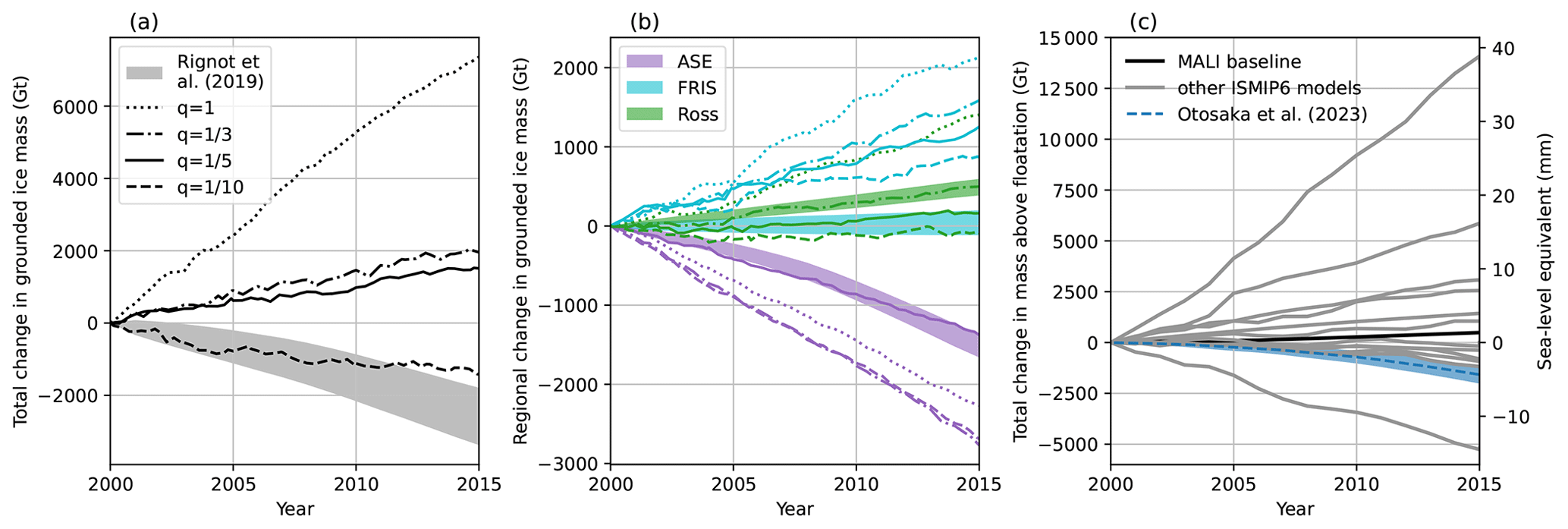
Figure 2 (a) Total and (b) regional change (see Fig. 1c for region definitions) in grounded AIS ice mass from four historical simulations with different values of the sliding law exponent. We used $q=\mathrm{1}/\mathrm{5}$ in our baseline simulations (solid lines), as it provided the best trade-off between whole-AIS and regional mass change. Shaded areas represent 2σ range of observations from Rignot et al. (2019). (c) The MALI baseline ISMIP6 historical run ($q=\mathrm{1}/\mathrm{5}$) in the context of the other ISMIP6 historical runs and the sea-level contribution estimate of Otosaka et al. (2023) with 2σ uncertainties.

After the above changes, we integrated the model forward for ten years using the static historical forcing to allow the ice geometry to relax. In this relaxation run, melt rates in the ASE were set to zero to prevent the Thwaites Glacier grounding line from retreating. The relaxed state is considered our initial condition for the historical simulations, corresponding to the year 2000 (Fig. 1).

2.3 Experimental design

2.3.1 ISMIP6 Antarctica 2300 baseline configuration

We treat the model configuration submitted to the ISMIP6-Antarctica-2300 ensemble (Seroussi et al., 2024) as our baseline configuration (called DOE MALI 4 km in Seroussi et al., 2024). Our baseline configuration includes a fixed calving front, meaning that any ice advected beyond the initial (ca. 2000) calving front is immediately calved away, but the calving front may retreat from its initial position due to surface or basal melt, or due to imposed hydrofracture in some experiments. Submarine melting is treated in two ways. We employ the ISMIP6 MeanAnt median non-local quadratic melt parameterization for melt below ice shelves (Jourdain et al., 2020), and the melt undercutting parameterization of Rignot et al. (2016) for melting of grounded marine termini, which comprise roughly 38 % of the coastline of Antarctica (Drewry et al., 1982). In our historical simulation, melting at grounded marine termini accounts for about 6 % of the total submarine melt flux. For the sub-shelf melt parameterization, given the prescribed MeanAnt melt sensitivity parameter (γ₀), we tuned the δT parameter for each sector to fit the overall ice-shelf melt flux from Rignot et al. (2013) when using thermal forcing from the observationally-based 1995–2017 ocean climatology provided by ISMIP6. We chose to define basins that incorporate the entire catchments of the Filchner-Ronne and Ross ice shelves to avoid sharp transitions in our tuned δT values along an arbitrary boundary within the ice shelves. We note that these two sectors thus include portions of both East and West Antarctica, and an analysis that used smaller basins could provide different insights. Our calculated δT values are shown in Fig. B2, along with the reported values from (Jourdain et al., 2020) for comparison. For the undercutting parameterization, we assume subglacial discharge is zero – an unrealistic but conservative assumption justified by a lack of additional constraints – and we linearly interpolate the three dimensional thermal forcing fields provided by ISMIP6 to define the thermal forcing at the seafloor. For basal sliding, we recalculated C from the optimization to that for a more-plastic rheology using $q=\mathrm{1}/\mathrm{5}$ (as described by Hillebrand et al. (2022)) as we found this resulted in the best trade-off between total and regional grounded mass change during historical simulations (Fig. 2); other values overestimated mass loss from the ASE. The results that were submitted to ISMIP6-Antarctica-2300 (Seroussi et al., 2024) using this configuration are presented in Sect. 3.1. For ease of reading, we have adopted a naming convention for forcings that is more descriptive than the ISMIP6 experiment names (e.g., CCSM4-RCP8.5-2300 rather than expAE02); see Appendix B for equivalent ISMIP6 experiment names.

2.3.2 Extended simulations

As none of the simulations submitted to ISMIP6 had reached a steady state by 2300, we selected a subset of the baseline experiments (low emissions, high emissions with and without hydrofracture) to extend to 2500, and we extended the control simulation to the year 2775. We extended the control simulation out further to determine whether the present-day forcing is sufficient to cause substantial ice-sheet retreat in our configuration, which has been found by other studies using different ice sheet models and initialization and calibration procedures (Coulon et al., 2024; van den Akker et al., 2025). We used a threshold of 1 m sea-level contribution threshold to determine the length of the extended control simulation. We chose CCSM4-RCP8.5-2300 as the high-emissions scenario because of the large ice-sheet mass and area remaining at 2300 in our baseline simulations, which would allow for substantial change beyond 2300 (Figs. 3, 4). We chose UKESM-SSP1‐2.6-2300 because it is the only available low-emissions scenario run out to 2300. We extended the forcing to 2500 by randomly sampling forcing from the years 2280–2300, similar to the approach used by ISMIP6-Antarctica-2300 to extend the 21st century forcing out to 2300 in the “repeat” experiments.

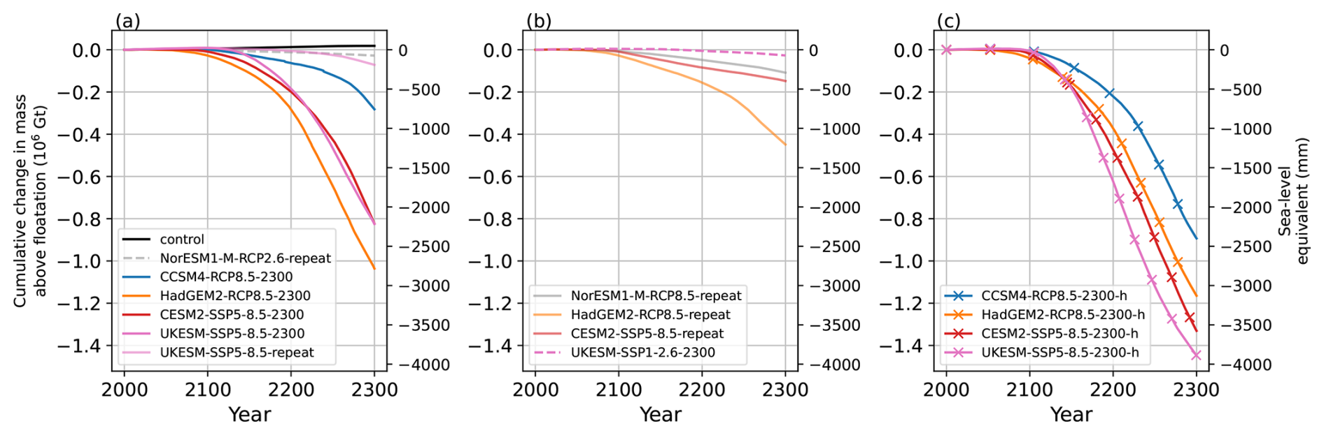
Figure 3 Results of the baseline ensemble submitted to ISMIP6-Antarctica-2300. (a) Tier 1 experiments, including control run in black. (b) Tier 2 experiments, with one extended SSP1-2.6 simulation and three repeat RCP8.5/SSP5-8.5 simulations. (c) Tier 2 experiments, with prescribed ice-shelf collapse based on liquid water on ice-shelf surfaces. We have adopted a more descriptive naming scheme than used by Seroussi et al. (2024); the equivalent experiment names from that study can be found in Fig. 4 and Table B1.

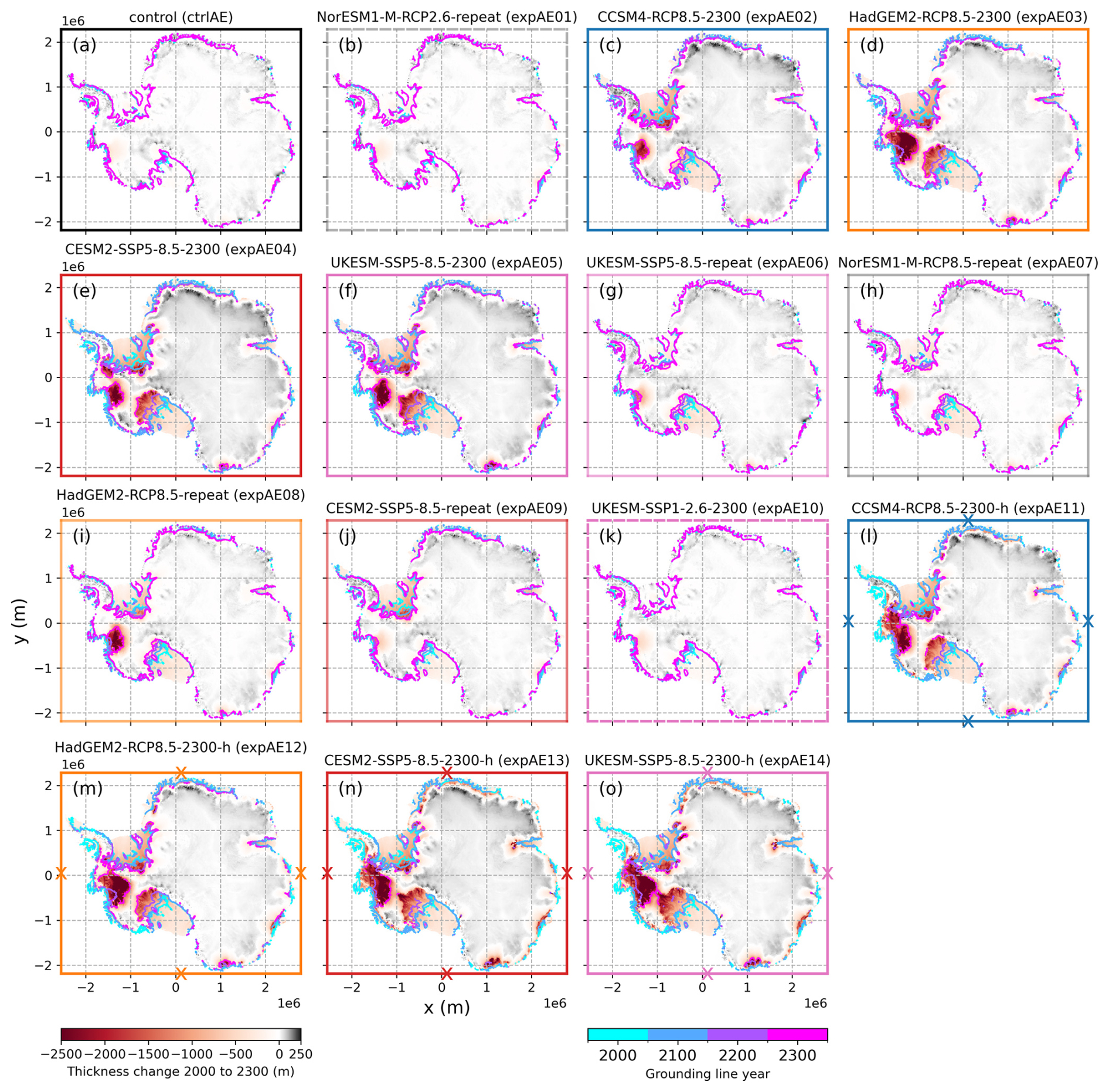
Figure 4 Maps of ice thickness change from 2000–2300 from the baseline ensemble submitted to ISMIP6-Antarctica-2300, with grounding line positions at 2000, 2100, 2200, and 2300. Axis border colors and line styles match the corresponding mass change curves in Fig. 3.

2.3.3 Parameter sensitivity experiments

The parameter sensitivity experiments were conducted using control, CCSM4-RCP8.5-2300, and HadGEM2-RCP8.5-2300 forcing, corresponding to ctrlAE, expAE02, and expAE03, respectively, in Seroussi et al. (2024). We chose the CCSM4 and HadGEM2 forcings because they were our low- and high-end mass loss high greenhouse gas emissions scenarios (RCP8.5/SSP5-8.5) in the baseline ensemble (Fig. 3). Running the experiments with the control forcing allows for separation of the forced from the unforced response to our modeling choices. However, as ISMIP6-Antarctica-2300 did not subtract control simulation drift from forced projections, the results we present here are also not drift-corrected. The experiments are summarized in Table 1.

Table 1 Summary of sensitivity experiments described in Sect. 2.3.3 and 2.3.4. Bold-face text indicates the baseline value or setting. All sensitivity experiments used CCSM4-RCP8.5-2300 and HadGEM2-RCP8.5-2300 forcing.

Sub-shelf melt sensitivity

We ran two sets of simulations with varying sensitivity of ice-shelf melt to ocean thermal forcing to determine the likely range of behavior due to uncertainties in ice-shelf melt. We used the 5th and 95th percentile values of the melt parameter γ₀ reported by Jourdain et al. (2020) for the non-local MeanAnt parameterization (9620 and 21000 m a⁻¹, respectively; our baseline ensemble uses the median value of 14 500 m a⁻¹), which we take to be a comprehensive range of values for this parameterization. For each value of γ₀, we recalculate the δT field to match observed melt rates from Rignot et al. (2013) for ca. 2003–2008 as in our baseline ensemble.

Sliding law exponent

We varied the sliding law exponent within a wide range from our baseline value of $q=\mathrm{1}/\mathrm{5}$ to determine the impact of a linear viscous (q=1), a “hard” (Weertman, 1957) ($q=\mathrm{1}/\mathrm{3}$), and a nearly-plastic ($q=\mathrm{1}/\mathrm{10}$) bed rheology on projected mass loss. We take this to represent a comprehensive range of this parameter, since q>1 is unphysical and $q=\mathrm{1}/\mathrm{10}$ is among the smallest values used in the literature and should behave similarly to smaller values (Gillet-Chaulet et al., 2016) and to a regularized Coulomb law for a given effective pressure (Joughin et al., 2019). We recalculated the basal friction coefficient field from the optimization for each of these choices of exponents as in our baseline ensemble. We acknowledge that bed properties vary widely beneath the real ice sheet, and that there is likely no one-size-fits-all sliding law.

2.3.4 Model fidelity sensitivity experiments

The model fidelity experiments were also conducted using the control, CCSM4-RCP8.5-2300, and HadGEM2-RCP8.5-2300 forcing scenarios. The experiments are summarized in Table 1.

Energy balance

We examined the sensitivity of our results to thermomechanical coupling by comparing our baseline configuration with a temperature-based thermal solver to simulations using an enthalpy formulation (Aschwanden et al., 2012; Hoffman et al., 2018), and another set of simulations in which the temperature field from the end of the ten-year relaxation run is held fixed throughout the entire simulation.

Stress balance approximation

We examined the sensitivity of the results to the choice of approximation to the Stokes equations by performing a set of simulations using a MOLHO formulation (e.g., Brinkerhoff and Johnson, 2015; Dias dos Santos et al., 2022), which is substantially less computationally expensive than the Blatter-Pattyn solver. We use the same basal friction coefficient field for the MOLHO simulations as in the Blatter-Pattyn simulations.

2.3.5 Ensemble and analysis of variance

We next construct a 72-member ensemble of MALI simulations to determine the likely range of sea-level contribution from the AIS under a high-emission scenario given parameter and Earth system model uncertainty. We use full-factorial sampling of the parameters listed in Table 2. Unlike in the sensitivity tests, we use all four RCP8.5 and SSP5-8.5 forcings provided by ISMIP6-Antarctica-2300 (CCSM4-RCP8.5-2300, CESM2-SSP5-8.5-2300, HadGEM2-RCP8.5-2300, and UKESM-SSP5-8.5-2300), and we include both cases with and without hydrofracture for each Earth system model (ESM). As above, we use the 5th, 50th, and 95th percentile values of the sub-shelf melt parameter, γ₀. We omit the linear basal friction law (q=1) due to its poor performance in historical simulations and large impact on projections, but we include values of $\mathrm{1}/\mathrm{3}$, $\mathrm{1}/\mathrm{5}$, and $\mathrm{1}/\mathrm{10}$. Due to considerations of computational cost, we use only the MOLHO formulation of the stress balance approximation, and we use only the temperature formulation of the energy balance. Each simulation was run on 8 GPUs and 8 CPU cores on the Perlmutter supercomputer at the National Energy Research Scientific Computing Center. For details of GPU performance and configuration with MALI, see Watkins et al. (2023).

Table 2 Parameters and values used in the ensemble described in Sect. 2.3.5. We construct a 72-member ensemble using full-factorial sampling of the given parameter values.

We use this 72-member ensemble for an analysis of variance (ANOVA) to estimate the relative importance of the sources of uncertainty in our projections. ANOVA is a statistical method that compares variance within groups and between groups to detect differences in group means and attribute variance to different sources (Girden, 1992; von Storch and Zwiers, 1999). For ANOVA results to be valid, the samples should be independent, the data in each group should be approximately normally distributed, and the variance within each group should be approximately equal. We perform the ANOVA analysis with the statsmodel v0.14.4 Python package (Seabold and Perktold, 2023), using Type II ANOVA.

The ANOVA method allows us to quantify the variance in our ensemble due to each individual parameter (ESM, γ₀, q, and hydrofracture), as well as the multi-way interactions between these terms. Unlike in the previous ISMIP6 studies that perform ANOVA on a multi-model ensemble (Seroussi et al., 2023, 2024) and thus combine all ice-sheet model related variance into a single term, we are able to determine the contributions of two individual parameters (γ₀ and q) to the total ensemble variance and rank the importance of these parameter choices relative to the choice of ESM forcing and hydrofracture setting.

3 Results

3.1 ISMIP6 Antarctica 2300 baseline results

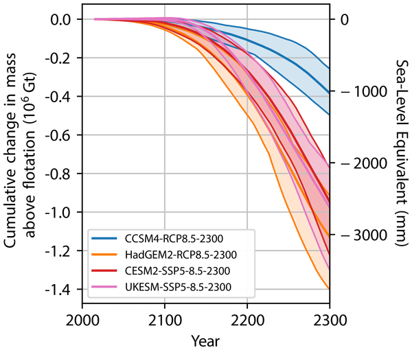
Figure 3 shows the change in mass above flotation and equivalent sea-level contribution from all experiments in our baseline ensemble, and maps of ice thickness change from 2000 to 2300 are shown in Fig. 4. Our control simulation, which used mean 1995–2017 surface mass balance and ocean thermal forcing, results in ∼ 40 mm sea-level equivalent (SLE) mass gain by 2300, while the inter-model spread in the ISMIP6 control runs range from 200 mm SLE mass loss to > 400 mm SLE mass gain (Seroussi et al., 2024). Our model drift is small compared with most of the forced simulations in our baseline ensemble, so we do not subtract the control run drift from the forced experiments. The Tier 1 experiments forced by extended RCP8.5/SSP5-8.5 simulations (Figs. 3a, 4c–f) predict between ∼ 0.8 and ∼ 2.8 m sea-level contribution by 2300, with the vast majority of mass loss occurring after 2100. All four of these simulations predict substantial grounding-line retreat at Thwaites Glacier (Fig. 4c–f), although with a wide range of magnitudes. Grounding-line retreat in the Filchner-Ronne Ice Shelf (FRIS) sector is limited in all four simulations, while there is substantial retreat in the Ross sector, again with a wide range of magnitudes. The two RCP8.5 CMIP5 experiments bound the range of overall mass loss from these experiments, with CCSM4-RCP8.5-2300 forcing giving the lower bound and HadGEM2-RCP8.5-2300 the upper bound on sea-level contribution. Meanwhile, the two SSP5-8.5 CMIP6 experiments yield very similar results to one another, predicting ∼ 2.2 m sea-level contribution (SLC) by 2300, with some slight variations in earlier years. For the RCP2.6/SSP1-2.6 and repeat RCP8.5/SSP5-8.5 forcing scenarios, the mass loss is much lower, with five of the six simulations predicting < 500 mm SLC by 2300, while the HadGEM2-RCP8.5-repeat forcing leads to ∼ 1.2 m SLC.

Including ice-shelf collapse via hydrofracture using masks provided with ISMIP6 forcing in the RCP8.5 and SSP5-8.5 forcing scenarios increases sea-level contribution by up to a factor of three, but with substantial differences between the relative increase for each ESM. The largest relative difference occurs for the CCSM4-RCP8.5-2300 forcing, increasing predicted sea-level contribution from ∼ 0.8 to ∼ 2.4 m, largely due to enhanced retreat of Thwaites and Pine Island glaciers and the Ross sector of West Antarctica (Fig. 4l). The smallest relative difference is found for the HadGEM2-RCP8.5-2300 forcing, which only increases from ∼ 2.8 to ∼ 3.2 m. For the two SSP5-8.5 CMIP6 forcings, the increase in mass loss due to ice-shelf collapse is substantial, with SLC increasing from ∼ 2.2 to ∼ 3.6 m for CESM2-SSP5-8.5-2300 and from ∼ 2.2 to ∼ 3.9 m for UKESM-SSP5-8.5-2300. In the UKESM-SSP5-8.5-2300-h scenario, an interior seaway has begun to open between the Amundsen and Ross seas by 2300 (Fig. 4o).

The experiments that use relatively weak forcings (i.e., the control historical forcing, repeat forcing, or SSP1-2.6 forcings) predict modest thinning in the ASE, some limited grounding-line retreat in the Ross and FRIS sectors, and modest thickening over most of the remainder of the continent (Fig. 4a, b, g–k). These include the control, NorESM1-M-RCP2.6-repeat, UKESM-SSP5-8.5-repeat, NorESM1-M-RCP8.5-repeat, CESM2-SSP5-8.5-repeat, and UKESM-SSP1-2.6-2300 forcings (experiments ctrlAE, expAE01, expAE06, expAE07, expAE09, and expAE10 in Seroussi et al. (2024)). The one exception is HadGEM2-RCP8.5-repeat (expAE08), which predicts grounding-line retreat in the ASE (Fig. 4i) and leads to ∼ 1.2 m SLC by 2300, which is within the range of the extended RCP8.5/SSP5-8.5 scenarios. This indicates that late 21st century ocean conditions could be sufficiently warm to lead to extensive collapse of Thwaites Glacier within a few centuries under a high emissions scenario. While our model fit to observations is among the best of the multi-model ISMIP6-Antarctica-2300 ensemble when quantified by ice thickness and velocity root mean square error (Fig. 2 in Seroussi et al., 2024) and have a modest bias in historical mass-change trend (Fig. 2), our SLC predictions fall roughly in the middle of the predicted range at 2300 (Fig. 4 in Seroussi et al., 2024).

3.2 Extended simulations

Results of our extended simulations are shown in Figs. 5 and 6. The extended control simulation predicts minor ice-sheet growth until ∼ 2400, after which it begins to lose mass (Fig. 5). By 2500, a widespread thinning signal relative to 2000 has started to become apparent at Thwaites Glacier, the Thwaites grounding line has begun to retreat substantially (Fig. 6a), and the ice sheet has started to lose mass relative to the ca. 2000 initial condition (Fig. 5). By the end of the simulation (2775), the ice sheet has lost a mass of 1 m SLE. In the UKESM-SSP1-2.6-2300-extended simulation, rapid retreat (hundreds of kilometers per century) of the ASE grounding line begins after 2300 (Fig. 6c), and the ice sheet has lost ∼ 0.9 m SLE by 2500, an order of magnitude greater than its contribution by 2300. In the CCSM4-RCP8.5-2300(-h)-extended simulations, the rapid mass loss continues at a rate similar to 2300, but begins to level off after ∼ 2425 in the case without hydrofracture and after ∼ 2350 in the case with hydrofracture, as the WAIS runs out of ice that is vulnerable to ocean forcing (i.e., grounded below sea level). Both of these simulations predict an interior seaway connecting the ASE, FRIS, and Ross sectors, beginning after 2400 in the case without hydrofracture, and before 2400 in the case with hydrofracture.

Figure 5 Time series of mass change for the four extended simulations.

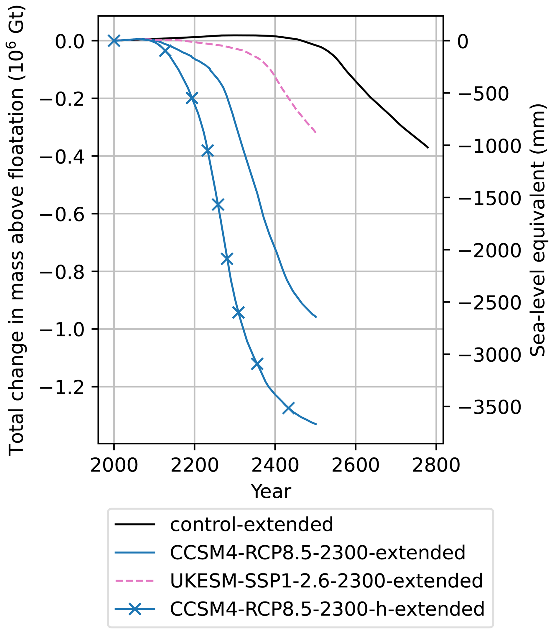
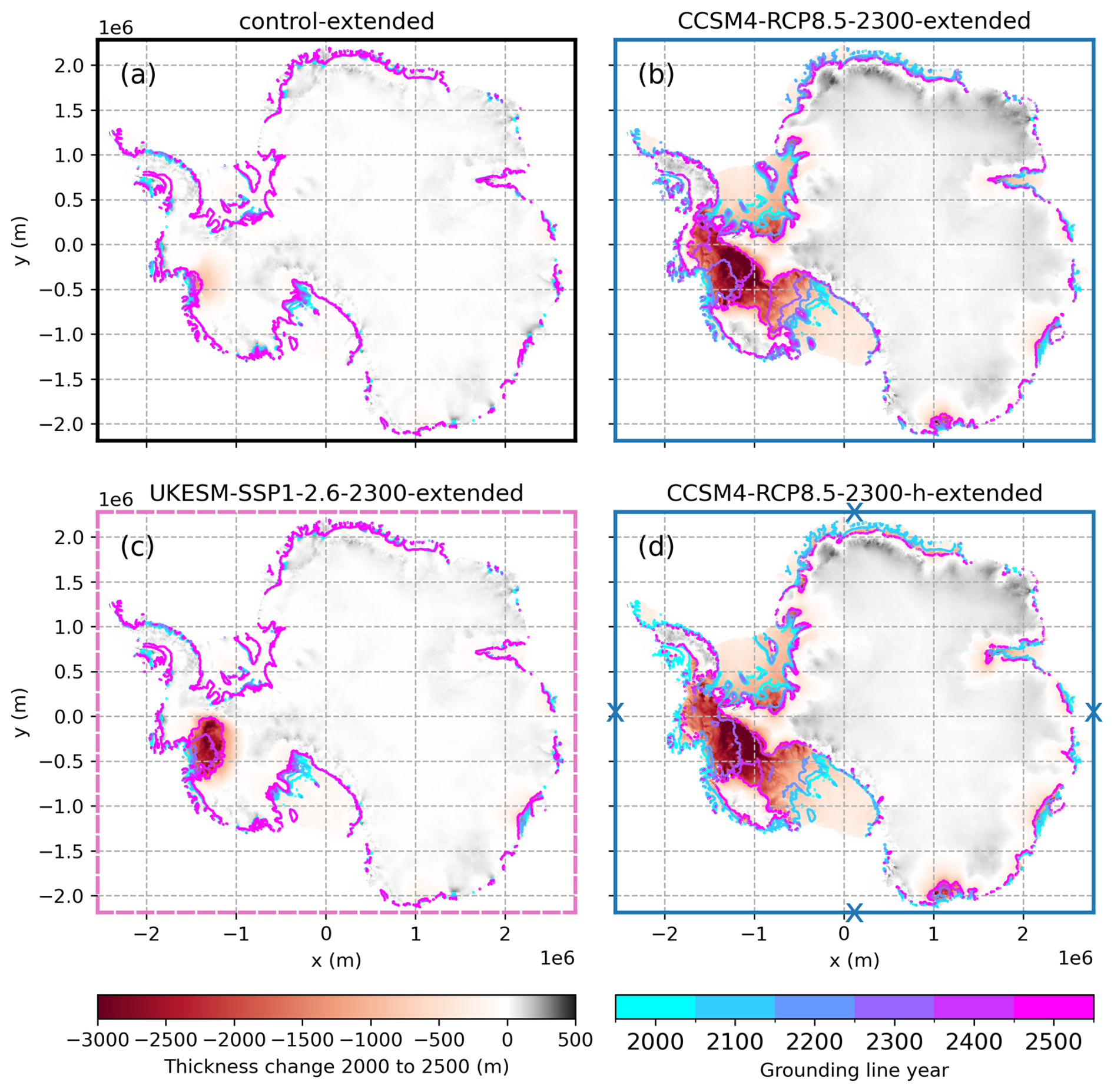
Figure 6 Maps of ice thickness change from 2000–2500 from the four extended simulations, with grounding line positions at 100-year intervals. Axis border colors and line styles match the corresponding mass change curves in Fig. 3.

3.3 Sensitivity to sub-shelf melt

Our simulations with 5th and 95th percentile values of the melt sensitivity parameter, γ₀, result in $\sim \pm$40 % and ∼ ±13 % differences from our baseline simulations for the CCSM4-RCP8.5-2300 and HadGEM2-RCP8.5-2300 scenarios, respectively (Fig. 7). When switching to the 5th percentile value of γ₀, total SLC by 2300 decreases from 0.8 to 0.5 m and from 2.8 to 2.5 m for CCSM4-RCP8.5-2300 and HadGEM2-RCP8.5-2300 forcings, respectively. When using the 95th percentile value of γ₀, total SLC by 2300 increases from 0.8 to 1.1 m and from 2.8 to 3.2 m for CCSM4-RCP8.5-2300 and HadGEM2-RCP8.5-2300 forcings, respectively. The three major basins largely exhibit the same sensitivity to the γ₀ value. In the control simulations, the SLC differs from our baseline by < 30 mm (Fig. C1). While the proper form of the sub-shelf melt parameterization might be highly uncertain, the calibrated range of γ₀ for this single parameterization using the MeanAnt calibration results in a 0.6–0.7 m range of sea-level equivalent mass change. This is modest relative to the multi-meter model-to-model differences for a given forcing scenario in ISMIP6-Antarctica-2300 (Seroussi et al., 2024).

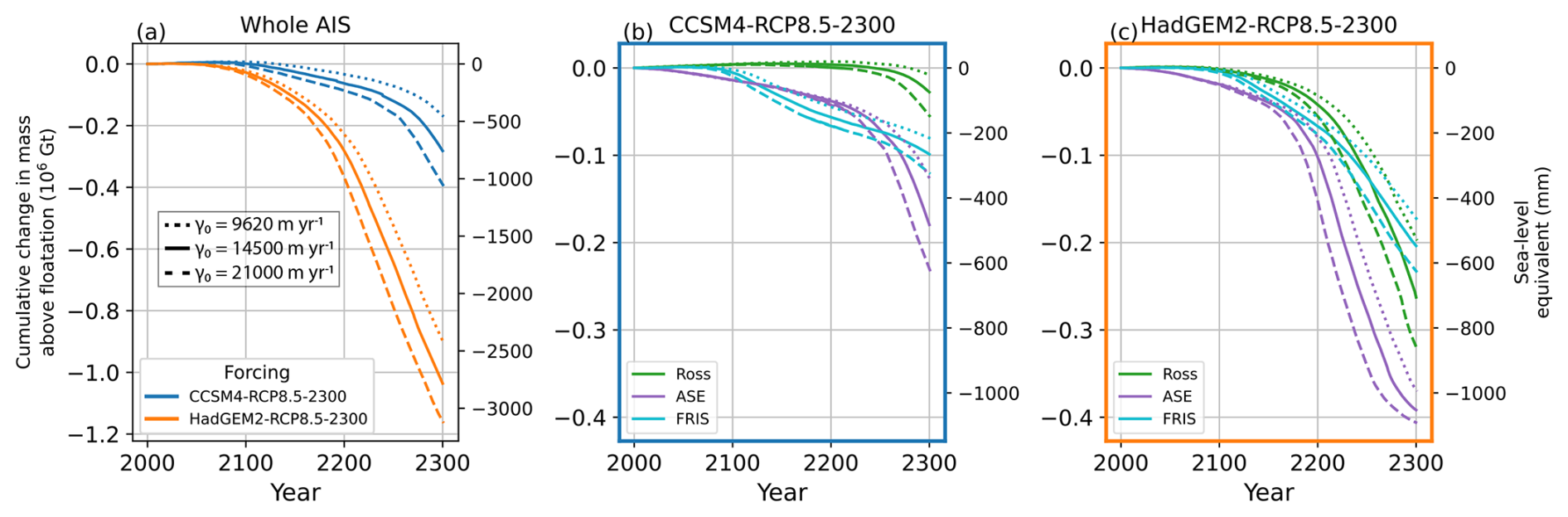
Figure 7 (a) Ice mass and sea-level equivalent change for ice-shelf melt sensitivity experiments. Experiments using CCSM4-RCP8.5-2300 and HadGEM2-RCP8.5-2300 forcings are shown in blue and orange, respectively. Line styles denote different values of γ₀. (b, c) Regional change for CCSM4-RCP8.5-2300 and HadGEM2-RCP8.5-2300 forcings, respectively. Line colors denote regions shown in Fig. 1; line styles correspond to the legend in panel (a).

Maps of thickness at 2300 relative to the corresponding baseline simulations are shown in Figs. 8 and D1. The major differences in thickness from the baseline scenarios are largely confined to the ASE and Ross sectors. While the sensitivity test simulations generally only differ quantitatively from the baseline simulations, the 95th percentile value of γ₀ leads to the opening of an interior seaway between the Weddell, Ross, and ASE sectors by 2300 when using HadGEM2-RCP8.5-2300 forcing, while the baseline scenario does not (Fig. 8d). It is possible that this seaway would open in the baseline scenario if it was run for a longer period.

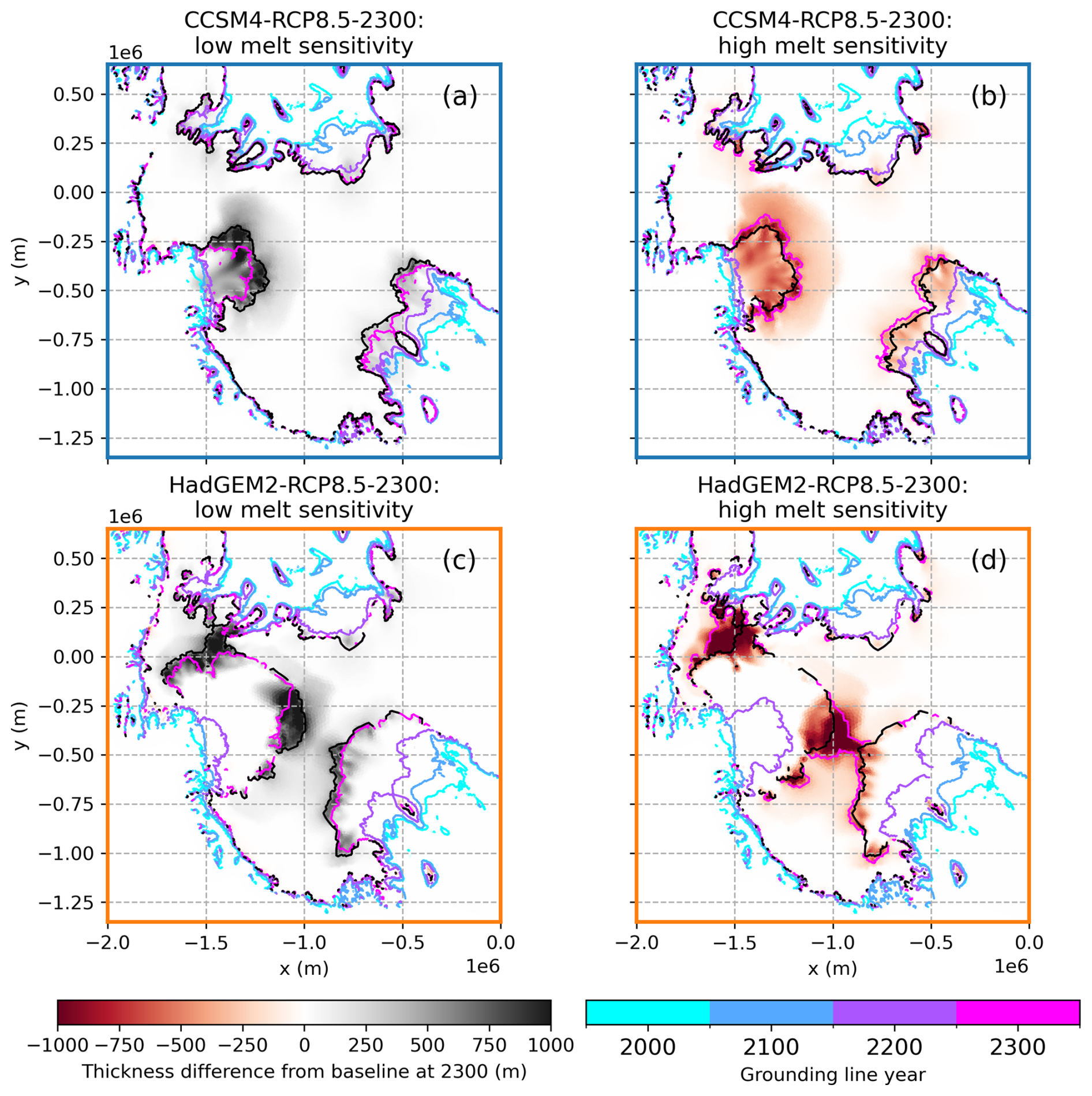
Figure 8 Maps of thickness in West Antarctica relative to baseline runs (γ₀= 14 500 m a⁻¹) at 2300 for low melt sensitivity (γ₀= 9620 m a⁻¹) (a, c) and high melt sensitivity (γ₀= 21 000 m a⁻¹) (b, d) experiments. Grounding lines from the sensitivity experiments are shown by colored curves at 2000, 2100, 2200, and 2300, while the grounding lines at 2300 from baseline simulations are shown in black. Results for the whole AIS are shown in Fig. D1.

3.4 Sensitivity to sliding law exponent

Our sliding law exponent experiments reveal a complex relationship between sliding, forcing, and SLC (Fig. 9). For the weaker CCSM4-RCP8.5-2300 forcing, the three smallest exponents ($\mathrm{1}/\mathrm{10}$, $\mathrm{1}/\mathrm{5}$, and $\mathrm{1}/\mathrm{3}$) result in very similar SLC (0.78–0.88 m) by 2300, although there is larger variability between 2100 and 2300. SLC is slightly greater when using $q=\mathrm{1}/\mathrm{3}$ and $\mathrm{1}/\mathrm{10}$ (13 % and 9 %, respectively) compared with $q=\mathrm{1}/\mathrm{5}$. Meanwhile, the q=1 exponent decreases SLC at 2300 by 73 %, and results in net ice-sheet mass gain until around 2200. There is a much larger spread between SLC for all exponent values for the stronger HadGEM2-RCP8.5-2300 forcing (1.4–3.3 m), with smaller exponents leading to more SLC by 2300, but with some complexity between 2150 and 2250. The linear sliding law reduces SLC at 2300 by 51 %, from ∼ 2.8 to ∼ 1.4 m, relative to our baseline value of $q=\mathrm{1}/\mathrm{5}$. In contrast, the hard-bed ($q=\mathrm{1}/\mathrm{3}$) scenario decreases SLC by 13 %, and the effectively plastic ($q=\mathrm{1}/\mathrm{10}$) scenario increases SLC by 14 %.

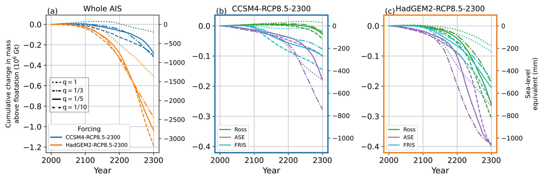
Figure 9 (a) Ice mass and sea-level equivalent change for sliding law exponent sensitivity experiments. Experiments using CCSM4-RCP8.5-2300 and HadGEM2-RCP8.5-2300 forcings are shown in blue and orange, respectively. Line styles denote different values of q. (b, c) Regional change for CCSM4-RCP8.5-2300 and HadGEM2-RCP8.5-2300 forcings, respectively. Line colors denote regions shown in Fig. 1; line styles correspond to the legend in panel (a).

The effect of the sliding law exponent on individual basins varies widely (Figs. 9b, c, C1b–d). For the FRIS and Ross basins, a smaller exponent leads to more SLC (or less mass gain) by 2300 in all forcing scenarios. FRIS contributes substantially to SLC for any value of the exponent in both forcing scenarios, with the exception of CCSM4-RCP8.5-2300 forcing with q=1. The Ross basin contributes < 200 mm to SLC for all values of the sliding law exponent under CCSM4-RCP8.5-2300 forcing, with q=1 resulting in net sea-level fall from that basin. Under HadGEM2-RCP8.5-2300 forcing, Ross and FRIS basins contribute similarly to net SLC for a given sliding law exponent, with a range of ∼ 200–800 mm.

The effect of the sliding law exponent for the ASE region is strongly non-linear in both forced and control scenarios (Figs. 9b, c, C1c). There is no direct relationship between SLC and the value of the exponent for either forcing scenario. Under CCSM4-RCP8.5-2300 forcing (Fig. 9c), the effectively plastic bed ($q=\mathrm{1}/\mathrm{10}$) scenario results in the smallest amount of SLC by 2300 (∼ 250 mm), while the hard-bed ($q=\mathrm{1}/\mathrm{3}$) scenario yields the most SLC (∼ 750 mm). The linear (q=1) and semi-plastic ($q=\mathrm{1}/\mathrm{5}$) bed scenarios result in the same amount of SLC (∼ 500 mm) at 2300, though with substantial differences from 2150–2300. During this interval, the q=1 simulation predicts more mass loss than the $q=\mathrm{1}/\mathrm{5}$ simulation. Under HadGEM2-RCP8.5-2300 forcing (Fig. 9c), all three values $\le \mathrm{1}/\mathrm{3}$ yield almost the same SLC from the ASE at 2300 (∼ 1050 mm) as the sector begins to run out of ice grounded below sea level, while the linear (q=1) bed yields ∼ 750 mm. In the simulations with control forcing, the ordering of sensitivity differs from the forced experiments, with q=1 yielding ∼ 350 mm SLC from the ASE by 2300, followed by $q=\mathrm{1}/\mathrm{3}$ (∼ 245 mm), $q=\mathrm{1}/\mathrm{10}$ (∼ 150 mm), and $q=\mathrm{1}/\mathrm{5}$ (∼ 115 mm). Overall, the sliding law exponent seems to dictate both the timing of the onset and the duration of rapid retreat, but in a way that is not predictable by the value of the exponent alone and is likely controlled by the interaction of the ice with complex bed topography and the spatial pattern of the forcing.

The strongly non-linear behavior with respect to the sliding law exponent is borne out in the spatial patterns of grounding-line positions and thickness differences relative to the baseline scenarios (Figs. 10, D2). For the simulations with CCSM4-RCP8.5-2300 forcing, the q=1 grounding line in the ASE at 2300 is virtually identical to the baseline $q=\mathrm{1}/\mathrm{5}$ simulation (Fig. 10a), reflecting the similar amounts of mass loss in Fig. 9. Likewise, the $q=\mathrm{1}/\mathrm{3}$ ASE grounding line – including Pine Island Glacier – has retreated much further than in the baseline scenario (Fig. 10b), reflecting its role in Fig. 9 as the highest mass-loss case. The $q=\mathrm{1}/\mathrm{10}$ grounding line has barely retreated at all by 2300 (Fig. 10c), reflecting the absence of rapid mass loss for that curve in Fig. 9b. Similarly, for the HadGEM2-RCP8.5-2300 scenarios, the q=1 grounding line has retreated much less than the $q=\mathrm{1}/\mathrm{5}$ grounding line (Fig. 10d), while the $q=\mathrm{1}/\mathrm{3}$ and $\mathrm{1}/\mathrm{10}$ grounding lines are close to the $q=\mathrm{1}/\mathrm{5}$ grounding line at 2300 (Fig. 10e–f), in keeping with their relative predictions of SLC from the ASE in Fig. 9c.

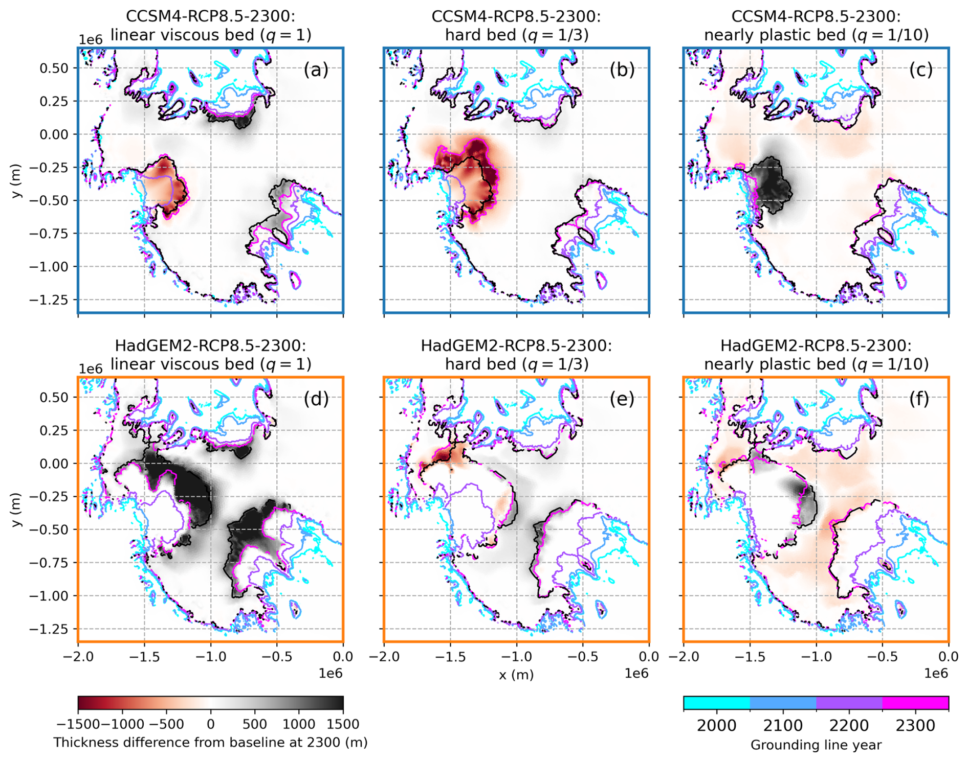
Figure 10 Maps of thickness in West Antarctica relative to baseline runs ($q=\mathrm{1}/\mathrm{5}$) at 2300 for experiments with q values of 1 (a, d), $\mathrm{1}/\mathrm{3}$ (b, e), and $\mathrm{1}/\mathrm{10}$ (c, f). Grounding lines from the sensitivity experiments are shown by colored curves at 2000, 2100, 2200, and 2300, while the grounding lines at 2300 from baseline simulations are shown in black. Results for the whole AIS are shown in Fig. D2.

3.5 Sensitivity to energy balance

We find that the temperature- and enthalpy-based formulations give nearly identical results, while using a fixed temperature field increases SLC by 88 % and 14 % for the CCSM4-RCP8.5-2300 and HadGEM2-RCP8.5-2300 scenarios, respectively (Fig. 11). The control simulation with fixed temperature loses mass equivalent to ∼ 180 mm SLC by 2300, compared with a net gain of 50 mm in our baseline control run (Fig. C1). In the CCSM4-RCP8.5-2300 scenario, the ASE grounding line retreats up to ∼ 200 km further by 2300 when using the fixed temperature field relative to evolving temperature (Figs.12, D3). For all forcing scenarios, using a fixed temperature field results in substantially more mass loss than an evolving temperature field. The magnitude of this effect varies from sector to sector, with a much larger effect in the ASE and Ross sectors and more muted impact in the FRIS sector for the forced scenarios (Fig. 11b, c). In the control simulations, both the Ross and FRIS are insensitive to the thermal solver, but the mass loss in the ASE increases by ∼ 150 % when using a fixed temperature field (Fig. C1). Meanwhile, the difference between the temperature and enthalpy formulations results in negligible difference in SLC. For HadGEM2-RCP8.5-2300 forcing, the constant temperature case leads to an open seaway connecting the Weddell, Amundsen, and Ross seas through central West Antarctica by 2300 (Fig. 12d), while the thermally coupled simulations only predict connection between the Amundsen and Weddell seas (Fig. 12c).

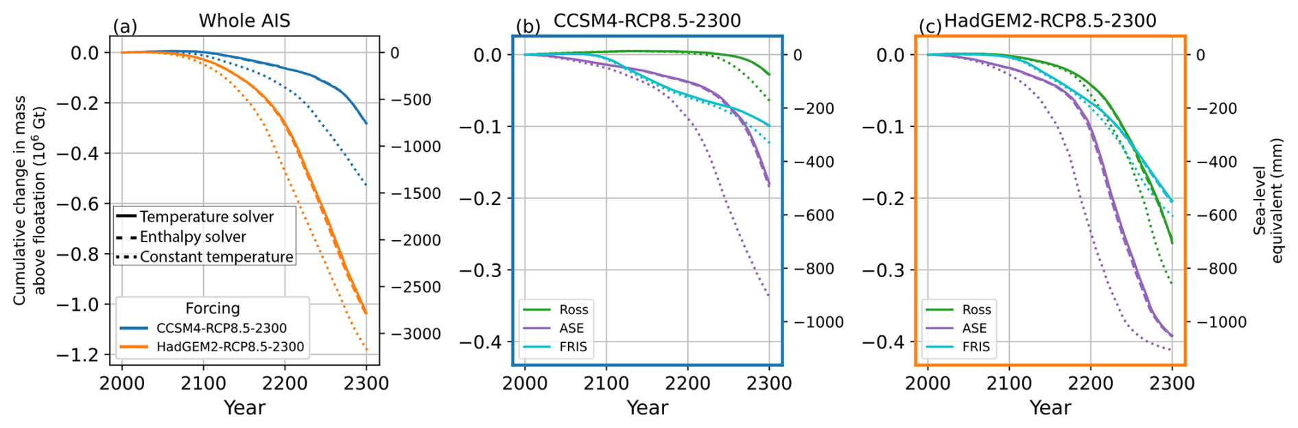
Figure 11 (a) Ice mass and sea-level equivalent change for energy balance sensitivity experiments. Experiments using CCSM4-RCP8.5-2300 and HadGEM2-RCP8.5-2300 forcings are shown in blue and orange, respectively. Line styles denote different solvers. (b, c) Regional change for CCSM4-RCP8.5-2300 and HadGEM2-RCP8.5-2300 forcings, respectively. Line colors denote regions shown in Fig. 1; line styles correspond to the legend in panel (a).

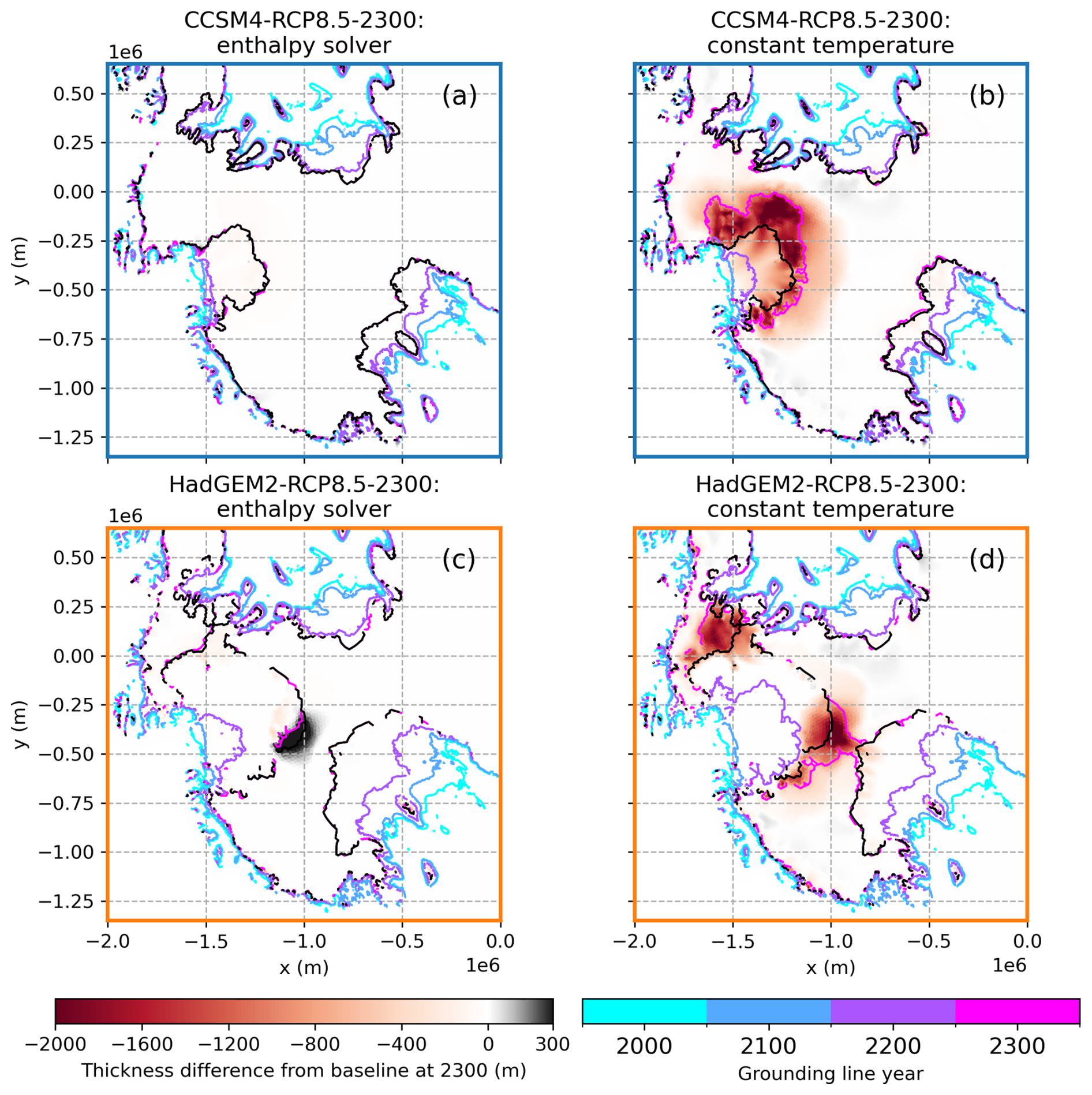
Figure 12 Maps of thickness in West Antarctica relative to the baseline runs using the temperature formulation at 2300, for experiments using the enthalpy formulation (a, c) and a fixed temperature field (b, d). Grounding lines from the sensitivity experiments are shown by colored curves at 2000, 2100, 2200, and 2300, while the grounding lines at 2300 from baseline simulations are shown in black. Results for the whole AIS are shown in Fig. D3.

Two reasons for this effect can be seen by examining temperature and flow speed along a transect down Thwaites Glacier for simulations with and without evolving temperature at 2150 (Fig. 13). First, melting at the base of the ice shelf removes warm ice in the thermally coupled case (Fig. 13a, c), leaving a cold, stiff, slower-flowing ice shelf. In the fixed-temperature case (Fig. 13b, d), the temperature field for each layer is simply applied to the evolving ice thickness using a terrain-following vertical coordinate, leaving a warm, soft, fast-flowing ice shelf. The warmer, softer shelf provides less back-stress to the ice upstream, leading to faster flow and therefore more grounding-line retreat and mass loss. Second, as the flow speed increases during grounding-line retreat, cold ice from upstream is advected toward the grounding line in the thermally coupled case, decreasing depth-averaged temperature of grounded ice relative to the fixed-temperature case and again leading to stiffer, slower-flowing ice. A similar advective cooling effect has been inferred for the Siple Coast ice streams (Hills et al., 2023).

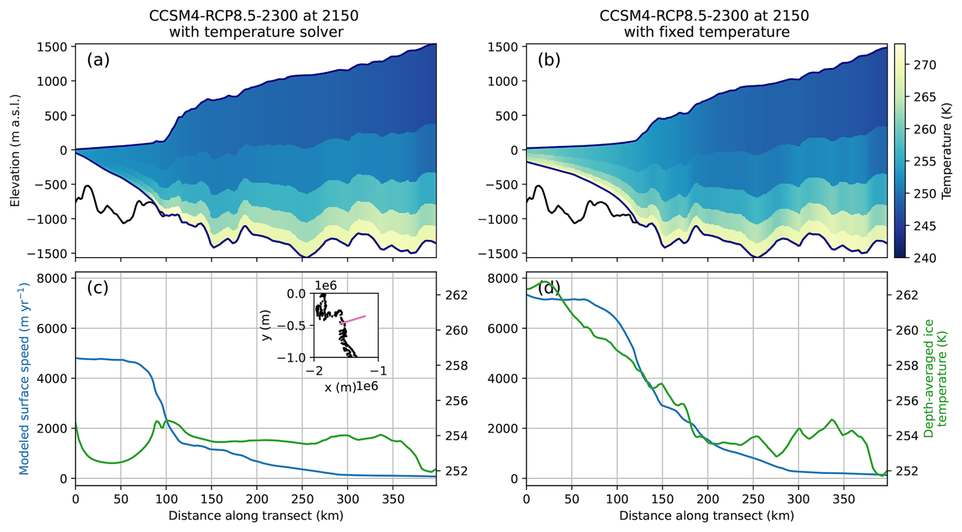
Figure 13 Modeled ice geometry and temperature (a, b) and surface flow speeds and depth-averaged temperature (c, d) taken from a transect down the center of Thwaites Glacier at 2150 from the CCSM4-RCP8.5-2300 simulations with an evolving temperature field (a, c) and with a fixed temperature field (b, d). Inset in (c) shows the location of the transect in pink, with the ca. 2000 ASE grounding line in black.

3.6 Sensitivity to stress balance approximation

The MOLHO solver predicts slightly higher flow speeds at the initial condition (Fig. A1) and a moderate increase in mass loss (Figs. 14, C1) relative to the three-dimensional Blatter-Pattyn solver. Of our three main basins of interest, the ASE displays the largest sensitivity to the choice of stress balance (Fig. 14b, c). For the CCSM4-RCP8.5-2300 forcing, using the MOLHO solver results in a ∼ 100–200 mm increase in SLC from the ASE region alone, while differences in the other regions are small. For the stronger HadGEM2-RCP8.5-2300 forcing, the FRIS region displays a slightly larger absolute increase in SLC than in the CCSM4-RCP8.5-2300 scenarios. The ASE still displays much greater sensitivity than either the Ross or FRIS regions, with the onset of rapid retreat occurring several decades earlier when using the MOLHO solver. Once rapid retreat initiates, however, the rate of SLC is largely the same between the MOLHO and Blatter-Pattyn simulations. This also results in a SLC difference of ∼ 100–200 mm for a given year between 2100 and 2300. Maps of thickness difference from the baseline simulations are shown in Figs. 15 and D4. Under CCSM4-RCP8.5-2300 forcing, the ASE has thinned more by 2300 in the MOLHO run than in the Blatter-Pattyn run, but the two are qualitatively similar (Fig. 15a). Under HadGEM2-RCP8.5-2300 forcing, the MOLHO stress balance predicts an interior seaway connecting the Weddell, Ross, and Amundsen seas, while the run using Blatter-Pattyn stress balance retains grounded ice that keep the Ross Sea separate (Fig. 15b).

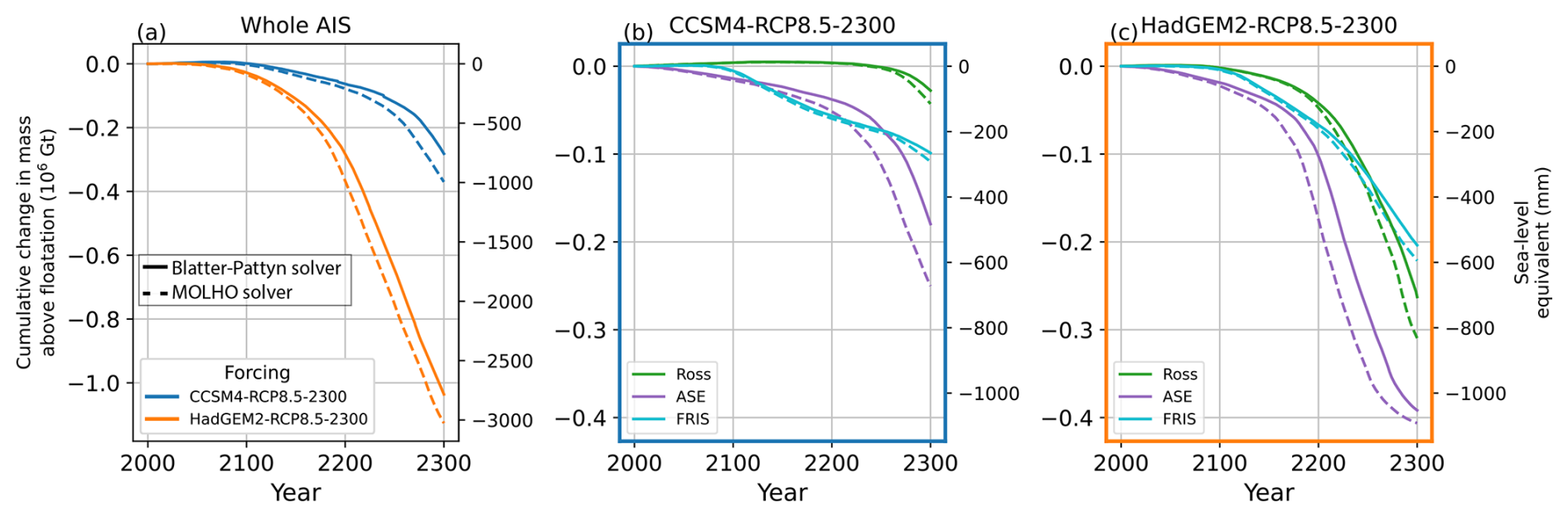
Figure 14 (a) Ice mass and sea-level equivalent change for stress balance approximation sensitivity experiments. Experiments using CCSM4-RCP8.5-2300 and HadGEM2-RCP8.5-2300 forcings are shown in blue and orange, respectively. Line styles denote the different solvers. (b, c) Regional change for CCSM4-RCP8.5-2300 and HadGEM2-RCP8.5-2300 forcings, respectively. Line colors denote regions shown in Fig. 1; line styles correspond to the legend in panel (a).

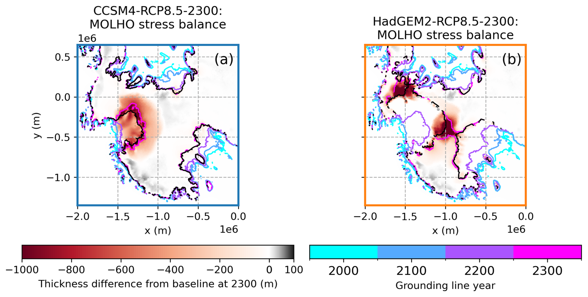
Figure 15 Maps of thickness in West Antarctica relative to the baseline runs at 2300, for experiments using the depth-integrated solver. Grounding lines from the sensitivity experiments are shown by colored curves at 2000, 2100, 2200, and 2300, while the grounding lines at 2300 from baseline simulations are shown in black. Results for the whole AIS are shown in Fig. D4.

3.7 Ensemble and analysis of variance

The results of our 72-member ensemble are shown in Figs. 16–19. In simulations without hydrofracture (Figs. 16–17), the ice sheet loses 0.6–3.6 m sea-level equivalent mass by 2300, with a large gap between runs using the CCSM4-RCP8.5-2300 forcing (0.6–1.4 m SLE) and those using the three stronger forcings whose contribution ranges overlap (2.0–3.6 m SLE). For all ESM choices, the Amery sector remains roughly in balance or slightly gains mass, while the other three sectors of interest lose substantial mass. The ASE is the largest source of mass loss on average for all four ESMs, with strong contributions from both the Ross and FRIS sectors for all ESMs except for CCSM4-RCP8.5-2300. In the CCSM4-RCP8.5-2300 runs, the Ross sector is only just beginning to contribute substantially by 2300 (Fig. 16b).

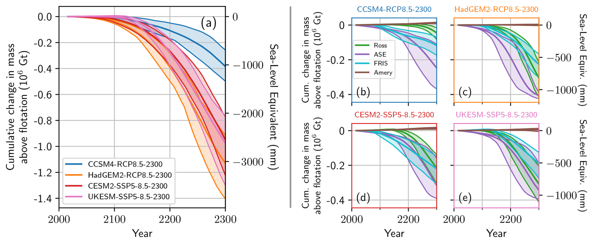
Figure 16 Results of ensemble without ice-shelf hydrofracture enabled. (a) Whole-AIS results, with curve color indicating the ESM used for forcing. The shaded regions represent the full range of simulations, with the curves representing the mean. (b–e) Regional results for each ESM forcing. Curve colors denote regions.

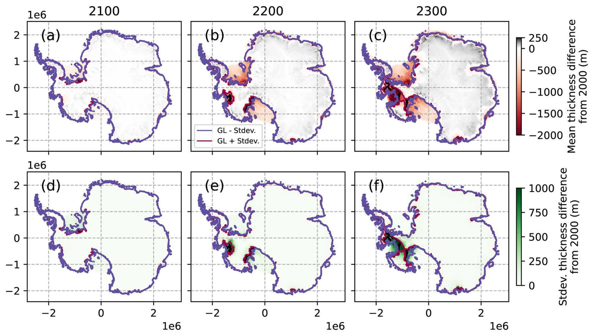
Figure 17 Maps of ensemble results without ice-shelf hydrofracture enabled. Mean ice thickness change since 2000 at 2100 (a), 2200 (b), and 2300 (c), with standard deviations in (d)–(f). Black curve represents grounding line calculated from mean thickness; dark purple and red curves are calculated using mean ±1σ thickness.

For the simulations without hydrofracture, on average, the ensemble predicts only modest changes by 2100, but major retreat of the WAIS by 2300 (Fig. 17). By 2200, the ensemble predicts substantial grounding-line retreat in the ASE, FRIS, and Ross sectors. The spread in ensemble members is small for the FRIS and Ross sectors. However, many ensemble members predict a close-to-modern-day grounding-line position in the ASE by 2200, while many others predict hundreds of kilometers of grounding-line retreat by this time. By 2300, the ensemble average predicts an open interior seaway between the ASE and FRIS regions, with some ensemble members also predicting full connection to the Ross sector. On average, the ensemble predicts moderate thickening of the EAIS, with thinning near the grounding line of the major outlet glaciers.

In simulations with hydrofracture, the ranges of mass loss from all four ESM forcings overlap, with a range of 2.1–5.1 m SLC by 2300 (Fig. 18a). CCSM4-RCP8.5-2300-h forcing still predicts the least mass loss on average, but CESM2-SSP5-8.5-2300-h and UKESM-SSP5-8.5-2300-h have overtaken HadGEM2-RCP8.5-2300-h as the scenarios with the largest average mass loss when hydrofracture is included. The Amery sector now loses mass under CESM2-SSP5-8.5-2300-h and UKESM-SSP5-8.5-2300-h forcing, but loses comparatively little to no mass in the CCSM4-RCP8.5-2300-h and HadGEM2-RCP8.5-2300-h scenarios. While the ASE remains the largest contributor for all ESM forcings, the Ross sector on average now loses at least as much SLE mass as the FRIS sector in all scenarios. The increase in mass loss from Ross under CCSM4-RCP8.5-2300-h forcing relative to the case without hydrofracture forcing is especially marked (green curves in Figs. 16b and 18b).

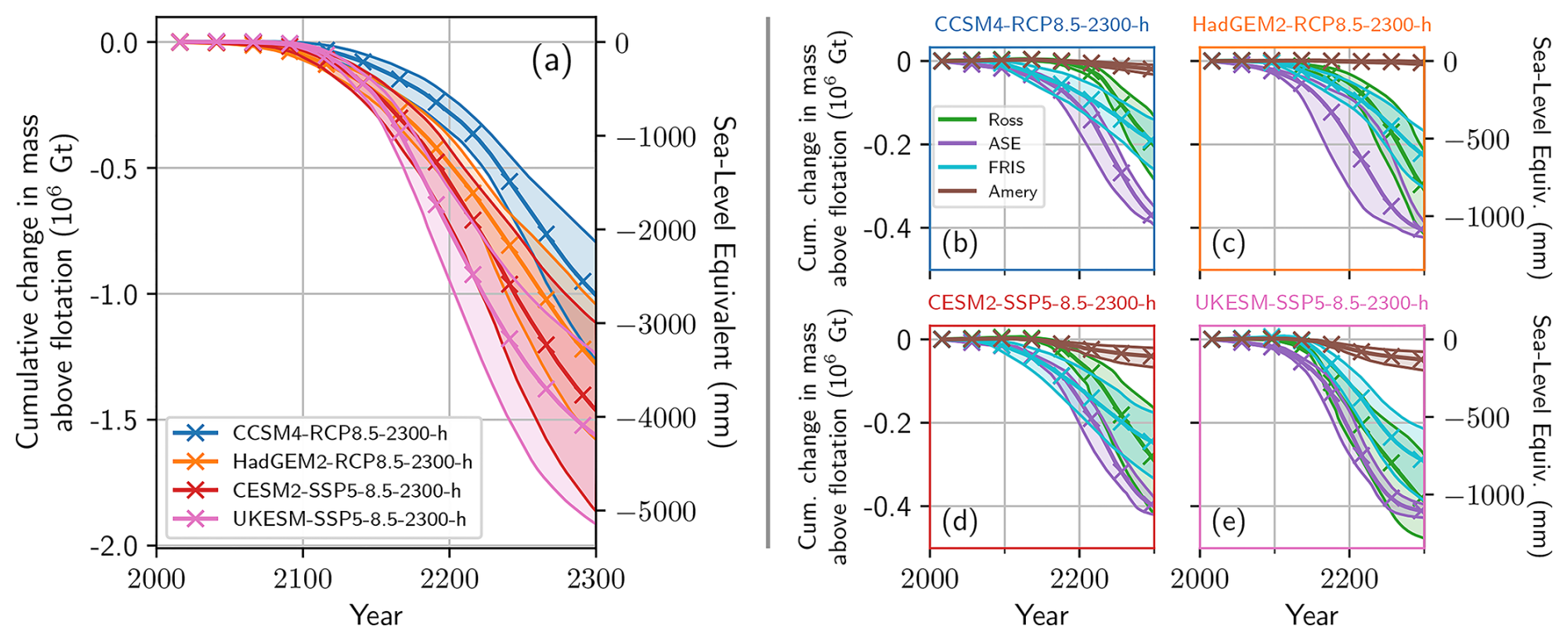
Figure 18 Results of ensemble with ice-shelf hydrofracture enabled. (a) Whole-AIS results, with curve color indicating the ESM used for forcing. The shaded regions represent the full range of simulations, with the curves representing the mean. (b–e) Regional results for each ESM forcing. Curve colors denote regions.

Grounding-line retreat by 2100 is still relatively modest in the hydrofracture-forced simulations (Fig. 19), as hydrofracture has yet to impact large areas of the ice shelves. However, by 2200 we see more retreat of the grounding line relative to the simulations without hydrofracture in the Ross and ASE, especially at Pine Island Glacier. By 2300, the ensemble average predicts a fully connected interior seaway between the ASE, Ross, and FRIS sectors, although many ensemble members still predict separation of the Ross sector from the others. The ensemble still predicts thickening of the interior EAIS, but with stronger thinning near the major outlet glaciers than in the simulations without hydrofracture (Fig. 17).

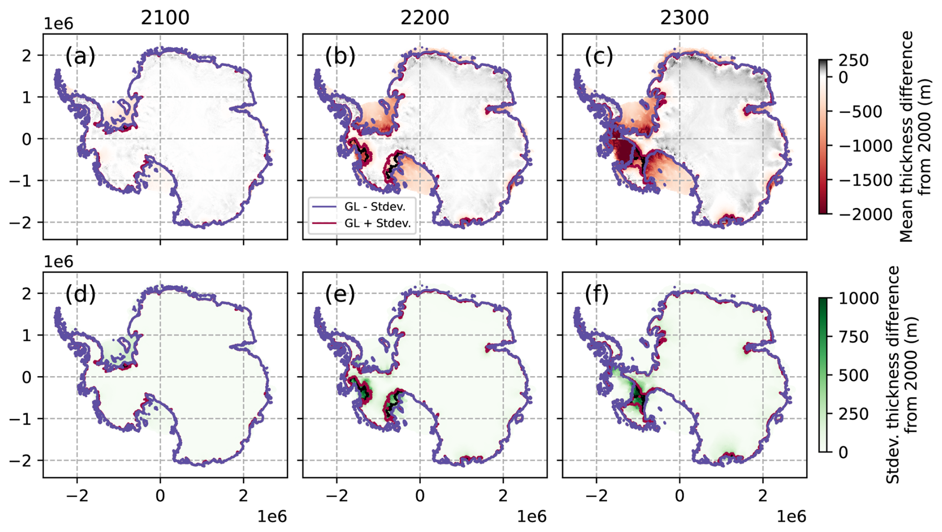
Figure 19 Maps of ensemble results with ice-shelf hydrofracture enabled. Mean ice thickness change since 2000 at 2100 (a), 2200 (b), and 2300 (c), with standard deviations in (d)–(f). Black curve represents grounding line calculated from mean thickness; dark purple and red curves are calculated using mean ±1σ thickness.

ANOVA results are shown in Fig. 20 for the whole ice sheet and in Fig. 21 for the four regions of interest. For the whole ice sheet, the choice of sliding law exponent dominates the ensemble variance for a few decades, after which the influence of the choice of Earth system model becomes dominant. The presence or absence of hydrofracture forcing grows rapidly as a source of variance after 2100, and roughly matches the variance explained by the choice of ESM forcing after ∼ 2125. Together, the ESM and hydrofracture terms account for ∼ 75 % of the ensemble variance for the last two centuries of the simulations. Despite the wide range of melt parameter γ₀ values we sampled within the constraints of the MeanAnt calibration, this parameter never explains more than ∼ 10 % of the variance in the ensemble.

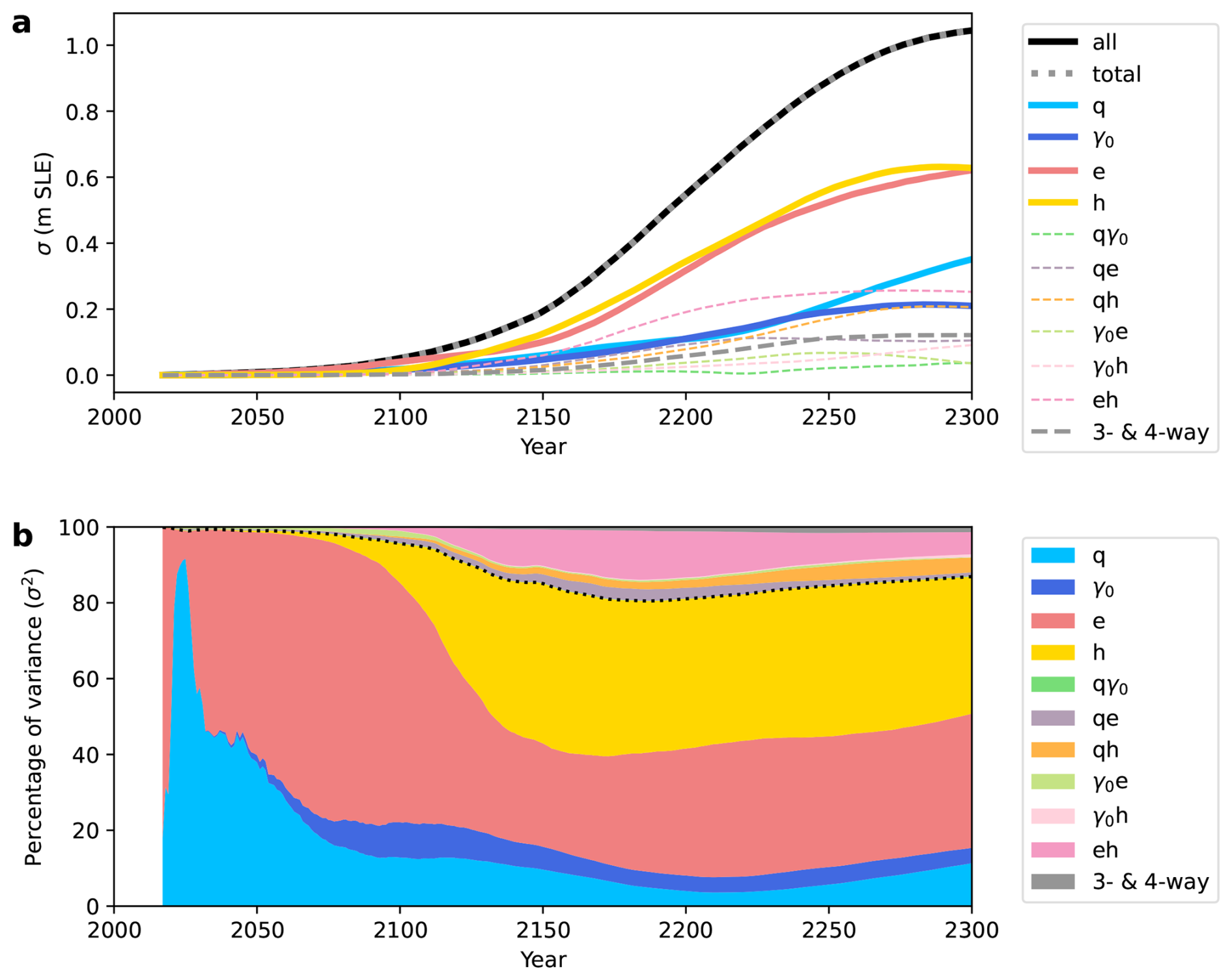
Figure 20 Contribution to uncertainty from different factors for the simulation period 2015–2300 from the 72-member ensemble using the MOLHO stress balance formulation. (a) Thick colored lines show standard deviation from sliding law exponent (light blue), γ₀ (dark blue), Earth-system model (denoted “e” in legend) used for forcing (coral red), and whether prescribed ice-shelf hydrofracture (“h” in legend) is included (yellow). Thin dashed lines indicate 2-way interactions. Gray dashed line indicates the sum of 3-way and 4-way interactions. Thick black line is the standard deviation calculated directly from all samples in the ensemble, and dotted gray line is the sum of all factors (1-, 2-, 3-, and 4-way) to uncertainty. (b) Percentage of total variance from each factor in (a). Black dotted line separates contributions from primary factors and interacting factors.

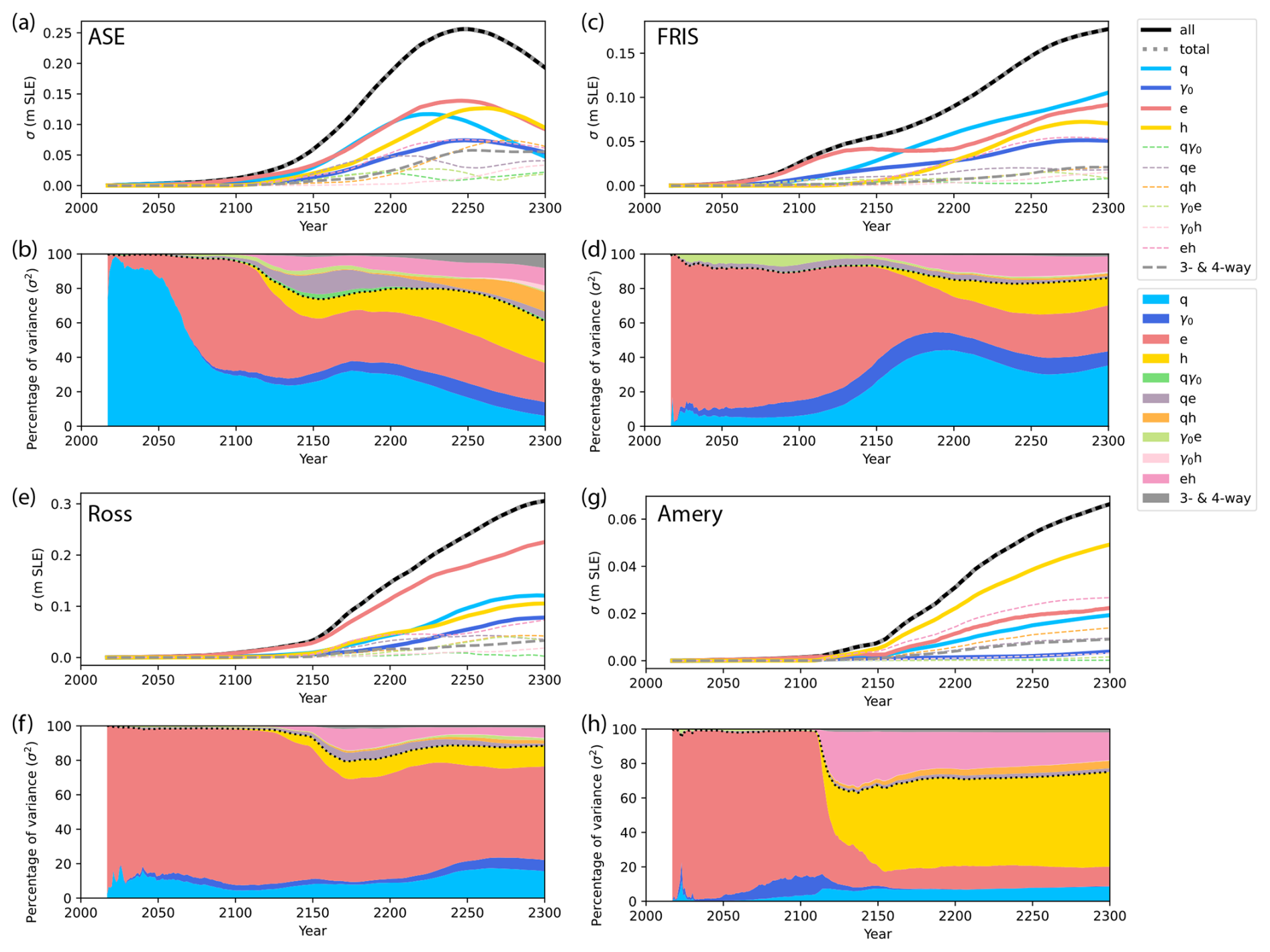
Figure 21 Same as Fig. 20 but for the ASE (a, b), FRIS (b, c), Ross (e, f), and Amery Ice Shelf sector (g, h).

The interaction between the ESM and hydrofracture forcings is the largest of the two-way terms, likely because some ESMs generate more surface melt than others, which makes them more likely to drive hydrofracture. There is some contribution as well from the two-way interaction between the basal sliding law exponent and the ESM and hydrofracture terms, respectively, qualitatively in keeping with our findings in the sensitivity tests (Fig. 9). The contributions of the other two-way interactions are essentially negligible, as are the three- and four-way interactions. The combined contribution of the interaction terms to the ensemble variance largely exceeds the combined influence of the individual sliding law exponent and melt parameter terms after ∼ 2150.

Our regional ANOVA results show marked contrasts between the four regions of interest (Fig. 21). In the ASE, the sliding law exponent plays a larger role, accounting for the majority of the variance until ∼ 2070 and remaining one of the largest terms until ∼ 2250. The two-way interaction terms play a larger role in the sector as well, accounting for > 40 % of the variance at 2300. ESM and hydrofracture forcing remain important terms, but combined they only account for ∼ 50 % of the variance at 2300. In the Ross sector, the choice of ESM forcing accounts for > 60 % of the variance through almost the entire simulation time and is by far the dominant term. The sliding law exponent and hydrofracture forcing terms are distant secondary contributors. The FRIS sector exhibits a large impact of the ESM choice until ∼ 2150, but after this the impact reduces, and hydrofracture forcing only becomes moderately important after 2200. The sliding law exponent is especially important late in the simulations, and the melt parameter is slightly more important than for other sectors, though its contribution remains below 20 %. For the Amery sector, the ESM forcing dominates the variance for the first century, after which hydrofracture rapidly takes over as the dominant term, in keeping with the results in Figs. 16 and 18. The two-way interaction between ESM and hydrofracture is especially large in this sector, likely reflecting a wide range of ESM-predicted surface melt available to drive hydrofracture. The basal sliding exponent accounts for < 10 % of the variance, and the impact of the melt parameter is negligible for the majority of the simulation time, except from ∼ 2075 to ∼ 2125.

4 Discussion

4.1 Extended simulations

Perhaps the most interesting outcome of the extended simulations (Figs. 5–6) is the fact that MISI-style retreat begins after 2300 for the UKESM-SSP1-2.6-2300-extended simulation and after 2500 for the control-extended simulation. The mass loss is dominated by thinning and retreat of the ASE (Fig. 6). This is in agreement with a body of work that shows that even modern-day melt rates in the ASE lead to dramatic retreat over long timescales (Joughin et al., 2014; Favier et al., 2014; Feldmann and Levermann, 2015; Reese et al., 2023; van den Akker et al., 2025). We note that we have not tested for the reversibility of this retreat, but the work of Feldmann and Levermann (2015), Hill et al. (2023), and Alevropoulos-Borrill et al. (2024) suggest that if melt rates are reduced in the near future this retreat may be avoided. However, while our control-extended simulation agrees with Stokes et al. (2025) on a very slight SLC at 2500 under continued present-day forcing conditions, our model predicts 1 m SLC between 2500 and 2775 under these conditions. And while our UKESM-SSP1-2.6-2300-extended (where SSP1-2.6 corresponds to roughly +1.8 °C above pre-industrial at 2100 (Fox-Kemper et al., 2021; Stokes et al., 2025)) simulation predicts an order of magnitude less SLC at 2300 than the +1.5 °C scenarios of both DeConto et al. (2021) and Stokes et al. (2025), by 2500 we predict ∼ 1 m SLC, in qualitative agreement with the 1.5 m SLC predicted by Stokes et al. (2025) by 2500 (see their Fig. 4). This could be due to the phenomenon noted by Seroussi et al. (2024) that once MISI-style retreat begins, different models tend to predict roughly the same rate of retreat, and the model spread mainly comes from the wide range of predicted onset times of retreat. Better calibration of ice-sheet models could thus help reconcile these different estimates (Aschwanden et al., 2021), although the timing of retreat could still be sensitive to remaining structural and parameter uncertainties.

4.2 Parameter sensitivity experiments

Our sub-shelf melt experiments (Figs. 7–8) show moderate sensitivity to the chosen value of the melt parameter γ₀, with a larger relative impact (±40 %) under the weaker CCSM4-RCP8.5-2300 forcing than under the stronger HadGEM2-RCP8.5-2300 forcing (±13 %). While these differences are not negligible, the spread due to parameter uncertainty is quite small compared with the spread due to forcing uncertainty, in keeping with the low contribution of the melt parameter to the ensemble variance (Figs. 20–21). There are no interesting non-linearity effects to speak of, only a slight shift in the timing of mass loss relative to the baseline simulations. An exploration of the structural uncertainty due to the choice of melt parameterization (e.g., including slope dependence (Lipscomb et al., 2021) or a plume parameterization (Hoffman et al., 2019)) or calibration target (e.g., Pine Island grounding-line melt sensitivity (Jourdain et al., 2020)) may uncover larger uncertainties in mass loss due to sub-shelf melt, but these are beyond the scope of this study.

Conversely, the choice between a linear and non-linear sliding law exponent, q, has a substantial effect on mass loss, with some strongly non-linear features (Figs. 9, 10). For the Ross and FRIS regions, mass loss increases with decreasing values of q, but the effect of q on mass loss from the ASE is quite different, potentially due to the more complex bed topography in this region. We observe complex behavior when varying the value of q that agrees strikingly well with the results of Schwans et al. (2023) and Parizek et al. (2013): the most plastic sliding law ($q=\mathrm{1}/\mathrm{10}$) leads to less retreat early in the simulation and can strongly delay the onset of MISI-style retreat of Thwaites Glacier. Surprisingly, for both CCSM4-RCP8.5-2300 and HadGEM2-RCP8.5-2300 forcing scenarios, the hard-bed Weertman ($q=\mathrm{1}/\mathrm{3}$) case predicts the most mass loss throughout most of the simulations, although the two more-plastic cases catch up in the final decades of the HadGEM2-forced simulation. This non-linear behavior is also apparent in the historical (Fig. 2) and control (Fig. C1) simulations, in which the baseline $q=\mathrm{1}/\mathrm{5}$ simulation loses the least mass in the ASE of all four choices of q. We note that this behavior cannot be attributed to initial condition uncertainty because all of our sensitivity tests begin from the same initial state with the basal friction coefficient rescaled based on the assumed value of q (see Sect. 2.3.3). Given the strong control of the sliding law exponent on the behavior of Thwaites Glacier, it is regrettable that this parameter was not reported systematically for the individual models contributing to ISMIP6 (Seroussi et al., 2020, 2024), as this could reasonably explain a large fraction of the very wide inter-model spread in the ASE.

We have limited our investigation of basal sliding to parameter sensitivity, but the structural uncertainty in the choice of the sliding law is likely at least as important. In a study of the effect of sliding law choices on projections of the ASE, Nias et al. (2018) and Brondex et al. (2019) found that Weertman-type relationships consistently predicted less mass loss than sliding laws that incorporated effective pressure. We have avoided using effective pressure-dependent sliding laws because current parameterizations of effective pressure are very crude and are extremely poor approximations far from the grounding line (Hager et al., 2022). Therefore, in simulations that predict tens to hundreds of kilometers of grounding-line retreat, effective pressure-dependent sliding laws may be strongly biased due to inaccurate effective pressure used to solve for the friction coefficient during model initialization. The simple parameterization of effective pressure suggested by Downs and Johnson (2022) could alleviate some of these issues, but it involves tunable parameters of its own, making the parameter space too large to explore here. However, we acknowledge that the Weertman-style sliding laws we use in this study have their own shortcomings.

4.3 Importance of thermomechanical coupling

While most modern ice sheet and glacier models regularly simulate thermal evolution coupled to mechanical ice flow, it is still somewhat common to use fixed temperature fields or even a uniform scalar value for ice temperature (cf. Goelzer et al., 2020; Rückamp et al., 2020; Seroussi et al., 2020; Choi et al., 2021; Seroussi et al., 2024; Holmes et al., 2025; O'Neill et al., 2025). This simplification is usually defended by the statement that the effects of thermomechanical feedbacks on ice flow are likely to be small; indeed, Seroussi et al. (2013) found that temperature evolution is relatively unimportant for predicting the evolution of the Greenland Ice Sheet to 2100. Our simulations have shown that this is unlikely to be the case for Antarctica, even for relatively short simulations. Even the sign of the sea-level contribution is different between our thermally coupled and fixed temperature simulations under CCSM4-RCP8.5-2300 forcing after just 50 years, although the magnitudes of SLC at that time are admittedly small. By 2100, SLC from the thermally coupled CCSM4-RCP8.5-2300 simulation is ∼ 0 mm, compared with ∼ 35 mm from the fixed temperature simulation. Our results suggest that a strong justification is needed to use a fixed temperature field for any but the shortest simulations, and that the insensitivity to thermal coupling should be demonstrated rather than assumed. At least three models (including MALI) out of thirteen total used fixed temperature fields in the first ISMIP6-Antarctica study to 2100 (Seroussi et al., 2020), and therefore may have overestimated mass loss. Conversely, the choice between our temperature- and enthalpy-based thermal solvers results in essentially negligible differences between the simulations over any time frame, indicating that the existence of thermal coupling is vastly more important than the details of the thermal solver. Of course, we cannot state definitively whether other models would exhibit a similar sensitivity to thermal coupling, or whether our finding would translate to the Greenland Ice Sheet, but our results indicate that future intercomparisons for Antarctica should consider requiring thermomechanical coupling as a prerequisite to participation.

We note that we have not examined the impact of vertical resolution on the effect of thermal coupling. We do not expect a strong resolution dependence, as our non-uniform vertical layer thickness results in higher resolution near the ice base where the effects are strongest (Fig. 13a, b). While we use only five vertical layers, borehole measurements of ice temperature in fast-flowing regions of Antarctica generally reveal smooth, low-gradient temperature profiles with depth (Engelhardt, 2004), which can be well approximated with a piecewise linear fit. Some temperature profiles in slow-flowing and divide-flow regions exhibit high curvature in the upper ice column (Talalay et al., 2020) that may be more difficult for our coarser near-surface layers to resolve. However, upper-ice temperatures in such slow-flowing regions likely have negligible impact on sea-level projections.

4.4 Importance of stress balance approximation

Our results show that the choice of stress balance approximation is important for the timing of the onset of rapid retreat in the ASE (Fig. 14), but is relatively unimportant for the other major regions of interest. The MOLHO model leads to earlier onset of retreat in the ASE than the Blatter-Pattyn model in both simulations, which leads to large differences in the predicted SLC at any given time after the early 22nd century. However, once rapid retreat has begun, the rate of retreat is mostly independent of the choice of stress balance approximation. Thus, it seems that the MOLHO model should be sufficient for sensitivity-style studies of the dynamics of the ASE region, in which determining the precise timing of the retreat is not a major goal. The story is more complex for the Ross region, with the HadGEM2-RCP8.5-2300 forcing displaying relatively large differences in mass loss between the MOLHO and Blatter-Pattyn solvers. For the FRIS region, the differences in mass loss between the solvers is small, and thus the computational savings provided by the MOLHO solver comes at very little cost to model accuracy. However, it should be acknowledged in studies using depth-integrated solvers that this could bias predicted mass loss and SLC. At the initial condition, the MOLHO solver predicts slightly higher flow speeds for grounded ice relative to the Blatter-Pattyn solver (Fig. A1) because in our configuration MOLHO predicts less vertical shear and thus more sliding for a given driving stress and friction coefficient field. In the shallow-shelf approximation (SSA), no stresses are balanced by vertical shearing, which is also likely to lead to more sliding and thus higher velocities than higher-order solvers. Thus, our finding here is consistent with comparisons between higher-order and SSA simulations for the Greenland Ice Sheet (Nias et al., 2023) and Thwaites Glacier (Yu et al., 2018), in which the SSA simulations predict higher SLC than runs using higher-order stress balance approximations. However, in the idealized MISMIP+ experiments, the stress balance approximation was found to be less important in general than the choice of the basal friction law (Cornford et al., 2020).

4.5 Importance of overall model fidelity

It is worth noting that our experiments with lower model fidelity (i.e., without thermal coupling and with the MOLHO solver) predict more mass loss by 2300 than the accompanying high-fidelity experiment. Different sectors exhibit different sensitivities to these model fidelity choices, but the overall effect on ice-sheet mass loss and SLC is substantial.

The literature on the response of the Antarctic Ice Sheet to climate forcing comprises results from a wide range of model fidelity, and modeling choices regarding fidelity are often made from considerations of computational cost rather than from demonstrated accuracy (e.g., convergence with respect to resolution). It has long been known that accurately simulating grounding-line dynamics requires very fine mesh resolution on the order of 0.1–1 km (Durand et al., 2009; Gladstone et al., 2012), but Williams et al. (2025) found that model resolution finer than 5 km is sufficient to accurately model the evolution of the ASE, although they acknowledge some model dependence of the required resolution. Most ice-sheet models (including MALI) lack adaptive mesh refinement, so resolution dependence is problematic for long simulations in which the grounding line is expected to retreat long distances. Given the high computational expense of simulating the entire ice sheet at high resolution with high fidelity models, we suspect that many models participating in ISMIP6 – including our own – are likely not fully converged with respect to resolution, which could be prohibitively expensive. Therefore, more targeted model intercomparison projects aiming for high fidelity for the ASE alone may be more trustworthy than the relatively low-fidelity whole-Antarctic simulations comprising ISMIP6.

Previous work with MALI has shown that a resolution of less than 1 km is required for a converged solution on a marine ice sheet-type domain when using the sub-element parameterization of grounding-line position used here (Hoffman et al., 2018). This is computationally impractical when using a higher-order Stokes solver on a continental domain when potential grounding-line retreat into the WAIS interior has to be taken into account in multi-century simulations. We undertook our baseline simulations with the knowledge that the model configuration was likely not fully converged with respect to resolution, which is a practical necessity in most Earth system modeling applications. Of the 43 different model configurations submitted in ISMIP6-Antarctica-2300, only five used a finer minimum cell spacing than our 4–20 km resolution (Seroussi et al., 2024): DC-ISSM (2–50 km), IGE-ElmerIce (1–50 km), UCSD-ISSM (3–50 km), UNN-Ua (1–40 km), and UTAS-ElmerIce (1–25 km). All of these configurations used the SSA stress balance, which is far less expensive than our Blatter-Pattyn solver (about a factor of 10; see Yu et al., 2018). The NCAR CISM submissions used a regular 4 km grid with a depth-integrated L1L2 velocity solver. The < 4 km resolution models all predicted lower SLC than our 4–20 km configuration in the ISMIP6-Antarctica-2300 ensemble, while the 4km NCAR CISM model predicted a higher (though overlapping) range of SLC compared with our model. It is thus tempting to suggest that higher resolution models predict less mass loss; however, several coarse resolution models with lower-fidelity stress balances (IMAU-UFEMISM: 30–200 km, hybrid stress balance; NORCE CISM: 8 km, hybrid; PIK PISM: 8 km, hybrid; UCM Yelmo: 8 km, L1L2; ULB Kori: 16 km, hybrid; and VUB AISMPALEO: 20 km, SIA + SSA) predict largely the same amount of mass loss as the five highest resolution models, while the 16 km hybrid LSCE-GRISLI model predicts nearly the same range as our 4–20 km baseline results despite its overall lower fidelity and worse fit to observations. We note that mesh resolution is only one component of numerical accuracy, but important details such as advection and time integration schemes were not systematically reported for the ISMIP6-Antarctica-2300 models. Thus, it is not clear that any single choice regarding fidelity can be deemed the most important when comparing across many different models. However, high resolution and accurate stress balance approximation do not necessarily translate to good agreement with observations (cf. Fig. 2 in Seroussi et al., 2024); conversely, good agreement with observations does not guarantee accurate future behavior for coarse resolution models with less accurate stress balances.

4.6 Sources of uncertainty in projections

Many ice-sheet characteristics and processes are highly uncertain and difficult to represent faithfully in numerical models. Modelers must choose between different input data sets to define model geometry (e.g., Fretwell et al., 2013; Morlighem et al., 2020; Pritchard et al., 2025). Initializing and calibrating ice sheet models is challenging, due to incomplete forcing data sets, nonlinear physics, and often sparse observational data. Many key physical processes are represented by relatively simple parameterizations that are unlikely to capture all the physics involved. For instance, numerous parameterizations exist to treat iceberg calving (e.g., Nick et al., 2010; Levermann et al., 2012; Pollard et al., 2015; Morlighem et al., 2016), basal friction (Weertman, 1957; Budd et al., 1979; Schoof, 2005; Joughin et al., 2019; Zoet and Iverson, 2020), and sub-ice-shelf melting (e.g., Hoffman et al., 2019; Jourdain et al., 2020; Lipscomb et al., 2021; Burgard et al., 2022), each with their own strengths and weaknesses in reproducing observations, and each with their own parameters to calibrate. Even in the highest fidelity models, the physics of ice flow is subject to uncertainties in form of the flow law and the value of the flow-law exponent (Millstein et al., 2022; Ranganathan and Minchew, 2024; Getraer and Morlighem, 2025; Schohn et al., 2025) and anisotropy due to crystal orientation fabric (Ma et al., 2010; Gerber et al., 2023), both of which are usually neglected due to computational challenges and limited observational constraints. No ensemble to-date has rigorously quantified the uncertainty due to all of these numerous sources, but the ISMIP6 ensembles have sampled widely among the common choices made by the major ice-sheet modeling groups.

In their analogous analysis of variance to what we present here, Seroussi et al. (2024) found that ice model uncertainty dominates variance at all times, being as large or larger than all other sources (Earth-system model, hydrofracture, and interaction terms) combined. Our study does not have a direct equivalent to their ice-sheet model uncertainty term because we are using a single ice-sheet model, in contrast to the 8 ice-sheet models used by Seroussi et al. (2024) in their ANOVA analysis. However, we do include many realizations of a single ice-sheet model through different values of the parameters q and γ₀. Seroussi et al. (2024) did not quantify parameter uncertainty directly, but their ice-sheet model uncertainty term includes parameter uncertainty along with structural uncertainty and initial condition uncertainty, as most choices were left up to each modeling group in the ISMIP6 protocol. The variance due to ESM and hydrofracture in our ensemble each reach 0.6 m by 2300 (Fig. 20), in close agreement with Seroussi et al. (2024); however, the ∼ 0.4 m variance (combining q and γ₀ contributions in quadrature) in our ensemble due to parameter uncertainty is much less than the ∼ 1.15 m variance due to ice-sheet model uncertainty in the ISMIP6-Antarctica-2300 ensemble.

It is not possible to partition ice-sheet model uncertainty from Seroussi et al. (2024) into these individual factors with their existing ensemble, but our analysis of uncertainty provides some insights into their relative importance. Our analysis samples two parameters (γ₀ and q), and finds that while q dominates uncertainty early in the simulations, beyond about 2100 uncertainty from these ice-sheet model parameters becomes less than 25 % of total variance, and uncertainty from the forcing (Earth-system model and hydrofracture) dominate (Fig. 20b). At the same time, ice-sheet model benchmarking intercomparisons (e.g., Cornford et al., 2020) have shown general agreement in ice dynamics for a given forcing between ice-flow models of varying fidelity, when models are run at sufficient spatial resolution (which, as noted above, may not be the case for many of the ISMIP6 ensemble members). In contrast, ice-sheet models are known to be sensitive to initial conditions (Seroussi et al., 2019) and the ISMIP6 ensembles have been shown to have historical behavior that deviates substantially from observations (Fig. 2 and Aschwanden et al., 2021). Thus, it could be that a large fraction of the large ice-model uncertainty reported by Seroussi et al. (2024) originates from initial condition uncertainty and does not necessarily indicate disagreement between ice-sheet models due to differences in model fidelity or parameter choices. However, as noted in Sect. 4.5, the impact of discretization error due to mesh resolution and numerical schemes is another potential source of uncertainty that warrants further investigation.

The spread in modeled SLC reported by Seroussi et al. (2024) comes partially from a wide range of predicted behavior at Thwaites Glacier, while the models largely agree on the extent of retreat in FRIS and Ross sectors. Long thought to be the region of Antarctica most sensitive to ocean warming (e.g., Hughes, 1977, 1981; Thomas, 1979), Thwaites Glacier remains stable (or nearly so) through 2300 in many of the simulations reported by Seroussi et al. (2024). Our baseline ensemble predicts among the largest amounts of grounding-line retreat at Thwaites by 2300 of the main simulations in that study, while matching observed rates of mass loss for the ASE relatively well (Fig. 2). Several other models participating in ISMIP6 displayed major differences at Thwaites Glacier between different modeling choices when using the same ice sheet model. The DC ISSM simulations predicted among the least retreat of Thwaites Glacier, while the UCSD ISSM simulations (which, incidentally, used a uniform scalar temperature field) predicted among the largest amounts of retreat. Similarly, the NORCE CISM simulations predicted small amounts of retreat, while the NCAR CISM simulations predicted similar amounts of retreat to our simulations. The VUW PISM simulations predicted almost no retreat of Thwaites Glacier by 2300, while the PIK PISM simulations predicted moderate amounts of retreat. We cannot say whether these differences are due to different model resolution, choices of physics and/or numerics, initialization procedures, or historical calibration, but it is a striking result that the same model can predict such different behavior of a glacier that has for so long been considered highly unstable.

We note that ANOVA is only as informative as the sources of uncertainty that were included. As noted elsewhere, we have not used a dynamic calving law, evolving basal friction, or glacial isostatic adjustment, and we have sampled no initial condition uncertainty. ANOVA also assumes the samples are independent, the data in each group are approximately normally distributed, and the variances within each group are approximately equal. For ISMIP6 applications like Seroussi et al. (2023, 2024) and this study, these conditions are unlikely to be rigorously satisfied. Further, the factors that were sampled likely do not capture the full range of uncertainty due to the small sample size within each factor. While we found the melt parameter γ₀ to have minimal impact on ensemble variance, we have not explored the Pine Island grounding line (PIGL) calibration of Jourdain et al. (2020) or other forms of melt parameterization that include ice shelf basal slope or plumes (e.g., Hoffman et al., 2019; Lipscomb et al., 2021; Burgard et al., 2022). Likewise, hydrofracture is merely treated as present or absent based on a threshold as in the ISMIP6 protocol, while in reality there is likely a range of impacts of surface meltwater on ice dynamics and calving, for instance through modulation of ice temperature (Hubbard et al., 2016), as well as uncertainty in threshold values (Trusel et al., 2015; Seroussi et al., 2024). Finally, the four ESMs we sample from ISMIP6-Antarctica-2300 are unlikely to capture the full range of uncertainty in ESMs. While we sample only an admittedly small portion of the true uncertainty, incorporating all sources of potential uncertainty into an ensemble with our model would be prohibitively computationally expensive. Thus, acceleration via statistical or deep learning emulators will be necessary in order to quantify the full range of uncertainty in sea-level projections from Antarctica (e.g., Edwards et al., 2021; Seroussi et al., 2023; Jantre et al., 2024; Rosier et al., 2025).

4.7 Limitations

Model initialization and calibration are immense challenges at the scale of an entire continent. We had to make judicious choices regarding calibration targets, given the constraints of computing time, human time, available observations, and model capabilities. For instance, we use the almost universally adopted approach of choosing a uniform value for the sliding law exponent, not because this is physically realistic, but because of the difficulty of calibrating a spatially varying exponent in a reasonable time frame. Likewise, some regions proved insensitive to reasonable changes to the basal sliding exponent q, which we treated as a tuning parameter, and were not possible to bring within the range of observational constraints. In some cases, this could be due to model resolution, as many glaciers on the Antarctic Peninsula, for instance, are unlikely to be sufficiently resolved on a 4 km mesh. In other cases, we had to balance trade-offs between regional and continental metrics based on expert judgment, such as choosing a sliding law exponent that better matched the observed mass loss from the ASE at the expense of a worse fit to the overall Antarctic mass budget (Fig. 2). Furthermore, the community-standard melt parameterization of Jourdain et al. (2020) also does not reproduce the observed or inferred patterns of ice-shelf melt (e.g., Adusumilli et al., 2020; Paolo et al., 2023), which may make it impossible and/or undesirable to fit mass change observations using only the basal sliding exponent. Finally, we had to make decisions regarding the datasets used to initialize and calibrate the model. For instance, we had to manually remove artifacts in seafloor topography that exacerbated spurious grounding-line advance. This was a case of a data issue (interpolation between incomplete bathymetry observations) compounding with a modeling issue (imperfect fit to flux divergence at the grounding line) to create a problem that could not be fixed by tuning model parameters. Improvements could be made to our initialization and calibration workflow by including flux divergence as a constraint in the inversion (e.g. Perego et al., 2014), by using Bayesian calibration (e.g. Wernecke et al., 2020; Aschwanden and Brinkerhoff, 2022; Felikson et al., 2023; Jantre et al., 2024), or by a transient optimization approach (e.g. Goldberg and Heimbach, 2013; Goldberg et al., 2015; Badgeley et al., 2025).

The large expense of these simulations limits the parameter space that we have been able to explore. Due to the limited number of simulations and the large portion of the parameter space left unsampled, we are unable to propagate uncertainties forward to create probabilistic projections of mass loss from the AIS. Acceleration via statistical or deep learning emulators (Edwards et al., 2021; Seroussi et al., 2023; Jantre et al., 2024; Rosier et al., 2025) could somewhat alleviate this issue, but large numbers of model simulations are still necessary for emulator training. However, using a space-filling ensemble design such as Sobol' or Latin Hypercube sampling to produce training data for emulators would be a more efficient way to sample the parameter space than the full-factorial design used for ANOVA.

We have explored the sensitivity of our AIS model configuration to parameters controlling sub-shelf melt and basal sliding, but we have not explored the structural uncertainty inherent in choosing the specific form of the parameterizations for each. In the case of the basal sliding law, we based our choices of parameterization and parameter values on common assumptions in the literature, rather than on the best available sliding law. There is no consensus on what the “best” sliding law is, but the common Weertman-style power-law used here certainly is not it. However, this allowed us to explore a wide range of parameter values without the added complexity of including evolving effective pressure, which currently has no good physical parameterization when the grounding line retreats far from its modern position (Hager et al., 2022). While more theoretically rigorous than the power-law relationship, regularized Coulomb friction laws (Schoof, 2005; Joughin et al., 2019) include effective pressure and additional parameters such as bump height and threshold velocities that are difficult to calibrate and likely vary spatially, making the parameter space extremely large. Likewise, we have chosen a community-standard sub-shelf melt parameterization (Jourdain et al., 2020) that includes a precalibrated parameter and its uncertainty. Many other sub-shelf melt parameterizations exist and could give different results (Hoffman et al., 2019; Jourdain et al., 2020; Lipscomb et al., 2021; Burgard et al., 2022; Lambert and Burgard, 2025). Exploring a number of different parameterizations for sub-shelf melt as suggested by Lambert and Burgard (2025) would likely greatly increase the variance due to ice-shelf melt in our ensemble.

In this work, we did not explore the sensitivity of the model to several processes that are known to be important, such as iceberg calving, evolution of material properties like ice damage or fabric, glacial isostatic adjustment, and subglacial hydrology. Regarding iceberg calving, our initial attempts to calibrate the von Mises stress-based calving law of Morlighem et al. (2016) against observed ice-shelf changes (Greene et al., 2022) proved prohibitively difficult, as the initial ice extent from BedMachine v2 (Morlighem et al., 2020) does not correspond to a given year across the whole continent. Calibrating calving laws to hold calving fronts in quasi-steady state (e.g., Wilner et al., 2023) might be a viable alternative in the future, but the utility of this exercise is questionable for the more dynamic regions like the ASE. Furthermore, current calving parameterizations are too simple to replicate the cyclical nature of tabular iceberg calving that accounts for most of the calving flux from the largest ice shelves (Greene et al., 2022). Therefore, we decided to ignore the effect of iceberg calving in this study, while acknowledging that it is likely to be a major driver of ice-sheet retreat in the coming centuries (e.g., Yu et al., 2019). However, we note that the hydrofracture forcing scenarios included in the baseline simulations and in our 72-member ensemble likely represent an upper bound on the impact of iceberg calving from floating ice. Ice damage is known to have a strong impact on bulk ice viscosity and thus on sea-level projections (Lhermitte et al., 2020; Ranganathan et al., 2025), but we do not include the impact of damage on ice viscosity in these simulations as we are not yet running MALI operationally with evolving damage and damage-viscosity coupling. Similarly, we take the almost universally adopted value of n=3 for the flow-law exponent, the generality of which has recently been called into question (Millstein et al., 2022; Ranganathan and Minchew, 2024), but which only a few recent modeling studies have treated as an uncertain parameter (e.g., Ranganathan and Minchew, 2024; Getraer and Morlighem, 2025; Rosier et al., 2025). We have explored the impact of GIA on our projections in another study (Han et al., 2025) and found the impact to be of a similar magnitude to the most impactful processes explored here (i.e., thermal coupling and basal sliding). There are likely non-linear interactions between GIA and other processes such as basal sliding, sub-shelf melt, and calving that could account for considerable uncertainty in projections, and this area warrants further investigation. The impact of subglacial hydrology on projections of ice-sheet change is an active area of research and development with MALI that will be addressed in future work.

5 Conclusions

We have conducted three new sets of simulations – extended simulations beyond 2300, one-at-a-time sensitivity experiments, and a 72-member ensemble along with an analysis of variance – to better understand and improve upon the model configuration that we used in the ISMIP6-Antarctica-2300 experiment (Seroussi et al., 2024). Our primary findings are as follows:

• In a SSP1-2.6 simulation extended to 2500 and a control (∼ present-day forcing) simulation extended to 2775, marine ice-sheet instability-style retreat begins at Thwaites Glacier after 2300 and 2500, respectively, leading to ∼ 1 m SLC by the end of the simulations. This corroborates other studies' findings that present-day rates of mass loss may lead to substantial SLC from the ASE over long timescales (Joughin et al., 2014; Favier et al., 2014; Feldmann and Levermann, 2015; Reese et al., 2023; Bett et al., 2024; Coulon et al., 2024; van den Akker et al., 2025).

• Varying the ice-shelf melt sensitivity parameter γ₀ within the 5th–95th percentile range found by Jourdain et al. (2020) for the MeanAnt parameterization results in a ∼ ±40 % and $\sim \pm$13 % difference in SLC from our baseline simulations for the CCSM4 and HadGEM2 RCP8.5 scenarios, respectively. This difference is greatly exceeded by the factor of 3.5 difference between the CCSM4 and HadGEM2 RCP8.5 baseline simulations. Our 72-member ensemble corroborates this finding, with uncertainty in γ₀ never accounting for more than ∼ 10 % of the ensemble variance.

• The model is sensitive to the choice between linear and non-linear basal sliding law exponent, q. A choice of $q=\mathrm{1}/\mathrm{10}$ (effectively plastic) leads to 2.3–4.1 times as much SLC by 2300 as a choice of q=1 (linear viscous). Excluding q=1 and using the more reasonable values of $\mathrm{1}/\mathrm{10}\mathrm{\le }q\mathrm{\le }\mathrm{1}/\mathrm{3}$ (hard-bedded), the sliding law exponent is a major contributor to the ensemble variance early in the simulations, but becomes a relatively minor contributor after ∼ 2070. However, there is variation in the sensitivity on a region-to-region basis. The sliding law exponent contributes more than half the variance in the ASE until 2070 and remains >20 % until 2250. In the FRIS sector, it accounts for ∼ 30 %–45 % of the variance after 2150, while never accounting for more than ∼ 20 % in the Ross sector or ∼ 10 % in the Amery sector.

• Ice sheet models must be thermomechanically coupled to produce credible results. Using a fixed-in-time temperature field increases SLC at 2300 by up to 88 % relative to our forced simulations with evolving temperature. However, the choice between the common methods for solving thermal evolution may be unimportant. The assumption that the effect of thermal evolution is small over short time-scales is likely highly case-dependent and should be used only if the insensitivity can be demonstrated for that particular case.

• In each experiment in which model fidelity is altered, the higher-fidelity configuration predicts less overall mass loss from Antarctica. The differences range from modest and possibly acceptable in the case of the MOLHO versus Blatter-Pattyn stress balance approximations (9 %–31 % at 2300) to extreme and likely unacceptable in the case of constant temperature versus thermomechanical coupling (14 %–88 % at 2300). In both cases, the stronger forcing leads to lower relative sensitivity to the choice of model fidelity.

• Our 72-member ensemble and analysis of variance show that forcing terms (choice of Earth system model and presence or absence of hydrofracture) dominate the overall uncertainty in our projections relative to parameter uncertainty. However, individual sectors of the ice sheet respond differently to forcing and parameter choices, and parameter uncertainty remains > 20 % of the variance for the ASE and FRIS sectors for a majority of the length our simulations.

• While multi-model inter-comparison ensembles like ISMIP6 (Seroussi et al., 2020, 2024) are useful for quantifying the spread of mass change projections across many modeling frameworks, the numerous model-to-model differences can obscure the reasons behind the discrepancies between model predictions. Sensitivity studies with a single model, such as presented here, are necessary to understand how individual modeling choices affect projections of sea-level change. While perhaps less interesting scientifically than multi-model studies, they are necessary documentation of the impacts of common assumptions.

Appendix A: Implementation of Mono Layer High Order (MOLHO) model

The MOLHO approximation is based on the weak formulation of the Blatter-Pattyn (or High Order) model, where the following ansatz is used for the trial and test velocity functions:

$$\begin{array}{}\text{(A1)}& \begin{array}{rl}& \mathit{v}(x,y,z)=\mathrm{\Phi }\left(z\right){\mathit{v}}_{\mathrm{b}}(x,y)+\left(\mathrm{1}-\mathrm{\Phi }\left(z\right)\right){\mathit{v}}_{\mathrm{s}}(x,y),\\ & \text{where}\mathrm{\Phi }\left(z\right)={\left({\displaystyle \frac{s-z}{H}}\right)}^{(n+\mathrm{1})}.\end{array}\end{array}$$

Here H, s and n denote the ice thickness, surface elevation and Glenn's law exponent, respectively. This expression can represent both the SIA and SSA solutions, as seen by choosing v_b=0 and v_s=v_b, respectively. While we use the basal and surface velocities v_b and v_s as primary variables, alternative equivalent formulations, e.g., using v_b and ${\mathit{v}}_{\text{sh}}:={\mathit{v}}_{\mathrm{s}}-{\mathit{v}}_{\mathrm{b}}$ as in (Dias dos Santos et al., 2022), are possible. The MOLHO approximation can be viewed as a 2.5D modal approach, where the solution in the vertical direction is approximated using just two modes.

This approximation has been proposed and explored in previous works, including those by Bassis (2010); Brinkerhoff and Johnson (2015); Dias dos Santos et al. (2022). We adopt the name MOLHO from Dias dos Santos et al. (2022), although our implementation in the MALI code differs from theirs. As in our Blatter-Pattyn discretization, we construct a 3D mesh of wedge elements by vertically extruding a triangulation of the 2D ice domain. For MOLHO, this extrusion consists of a single (mono) layer of wedges. We define tensor-product finite element on the wedges composing a classic linear nodal finite-element on the base triangle, and the 1D Lagrange finite-element in the vertical having the following basis functions (in physical space):

$$\begin{array}{}\text{(A2)}& {\mathit{\varphi }}_{\mathrm{0}}\left(z\right)=\mathrm{\Phi }\left(z\right),{\mathit{\varphi }}_{\mathrm{1}}\left(z\right)=\mathrm{1}-\mathrm{\Phi }\left(z\right).\end{array}$$

Volume integrals over each wedge are computed using a tensor-product quadrature: a 4th-order Gauss rule on the triangle and a 7th-order Gauss rule in the vertical. In contrast, Dias dos Santos et al. (2022) performs analytic integration along the z direction of the model weak form, after numerically evaluating a depth-averaged viscosity, yielding a coupled system of two 2D vector equations for the basal velocity v_b and shear velocity v_sh. This approach has the potential of being computationally more efficient, operating entirely on 2D data structures. Our choice of implementation was guided by its simplicity and ease of integration into the MALI codebase, essentially requiring the use of a specialized finite element. Ongoing development in MALI aims to eliminate the explicit generation of the 3D mesh by leveraging the tensor-product structure in the finite element implementation, which will reduce memory footprint and computational cost.

For the solver, we use the multi-grid preconditioner (Tuminaro et al., 2016; Watkins et al., 2023) developed for the Blatter-Pattyn model, that performs a semi-coarsening in the vertical direction exploiting the structure of the extruded 3D formulation.

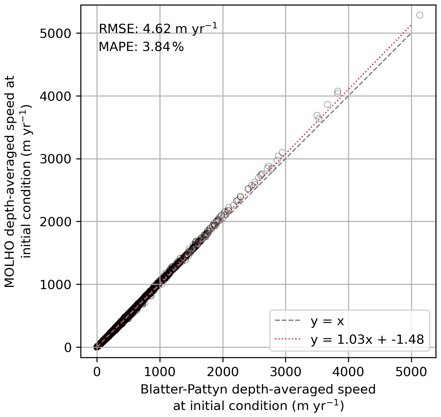
Figure A1 Depth-averaged speed from the MOLHO and Blatter-Pattyn solvers for all grounded ice cells at the initial condition. Red dotted curve denotes linear least-squares fit to the data (R²=0.9991). Dashed grey curve is 1:1 line. RMSE: root mean square error; MAPE: mean absolute percent error.

Appendix B: Forcings, boundary conditions, and experiments

Seroussi et al. (2024)

Table B1 Forcing names used in this paper, with the equivalent experiments from Seroussi et al. (2024). Our naming convention is: (Earth system model)-(emissions scenario)-(repeat late 21st century or calculated to 2300?)-(hydrofracture?)-(extended beyond 2300?). Forcings with -h include ice-shelf hydrofracture forcing. Four forcings were extended beyond 2300 using the methodology described in Sect. 2.3.2 and are denoted here with (-extended) to indicate that both the standard and extended versions were used.

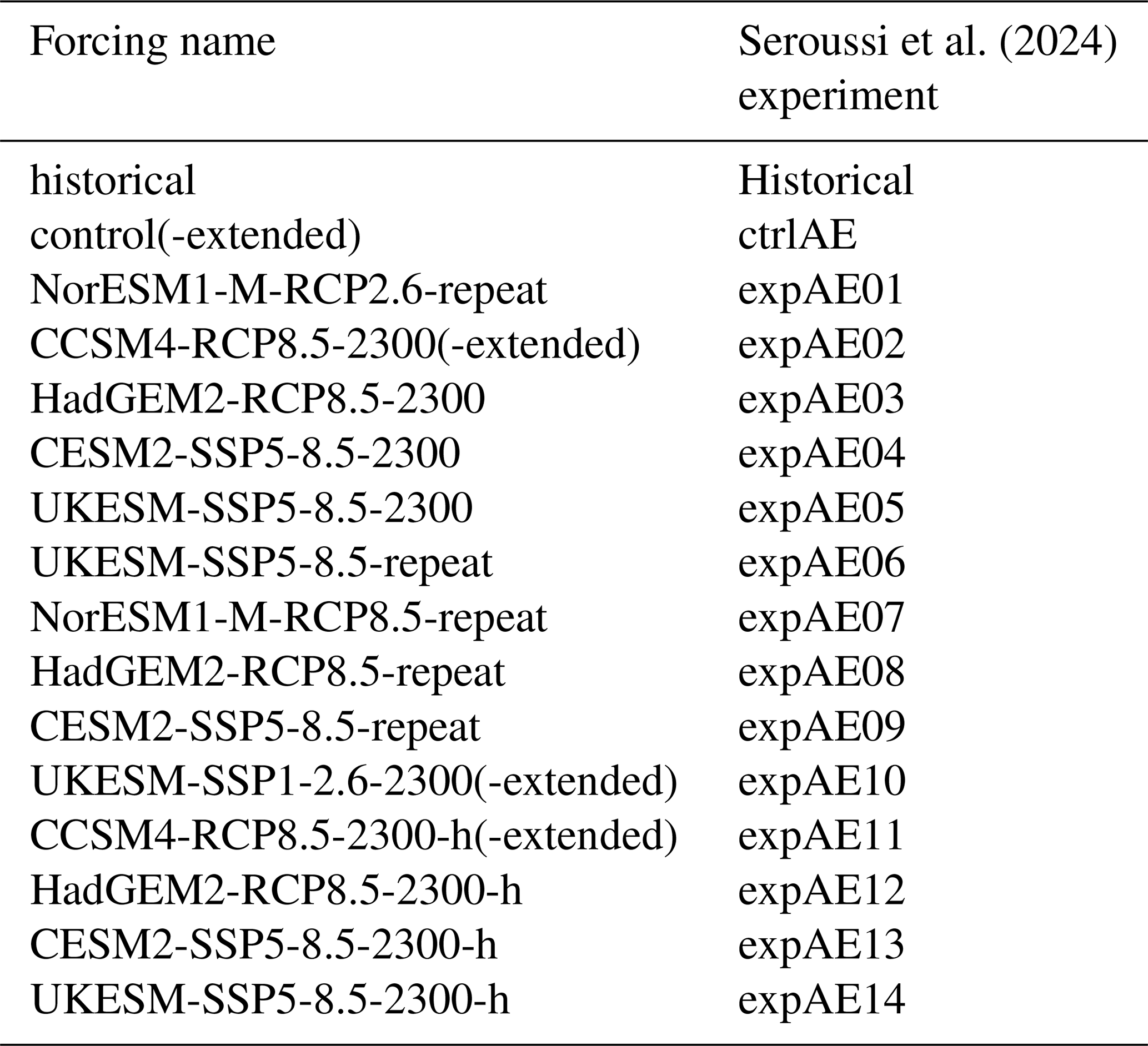
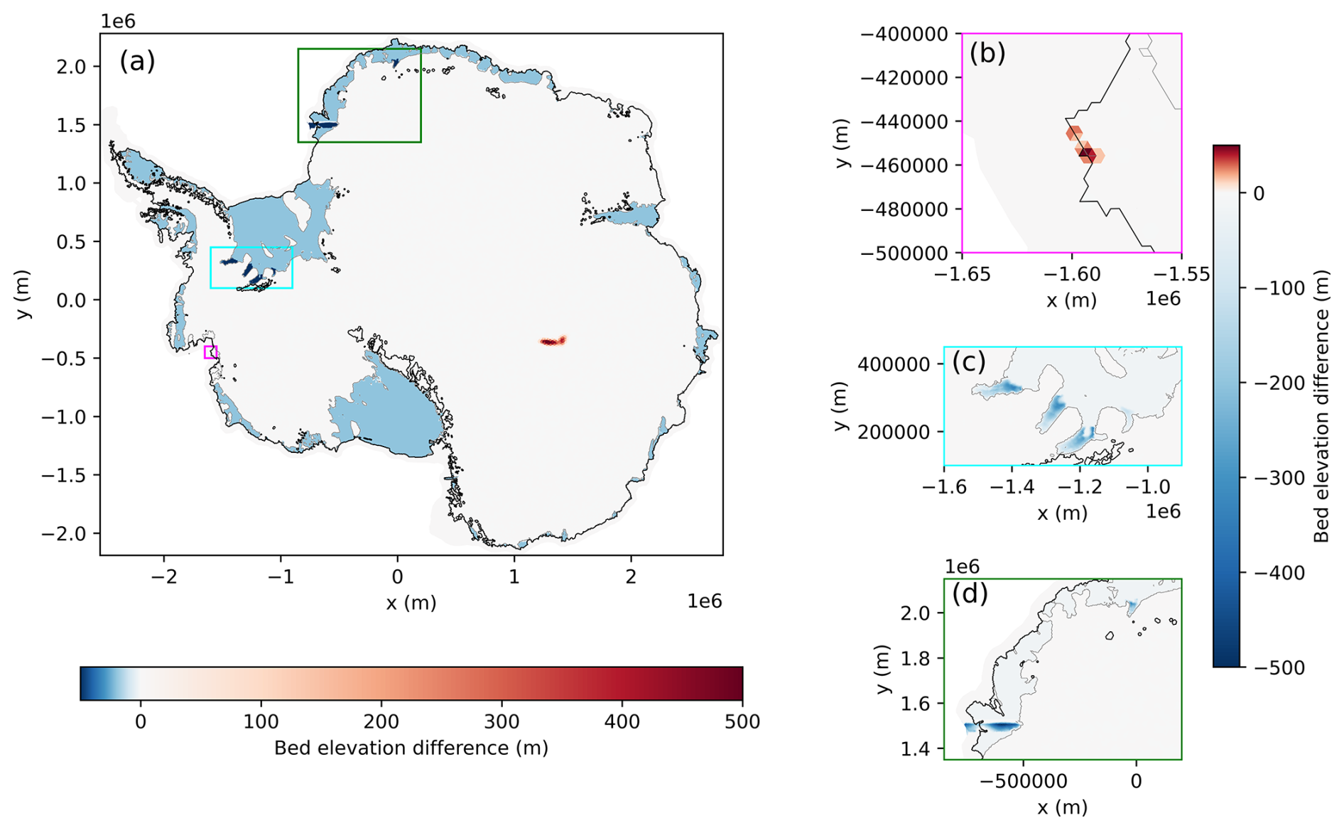
Figure B1 Difference in bed elevation used in MALI simulations relative to BedMachineAntarctica v2 (Morlighem et al., 2020). Negative values indicate a deeper bed in MALI.

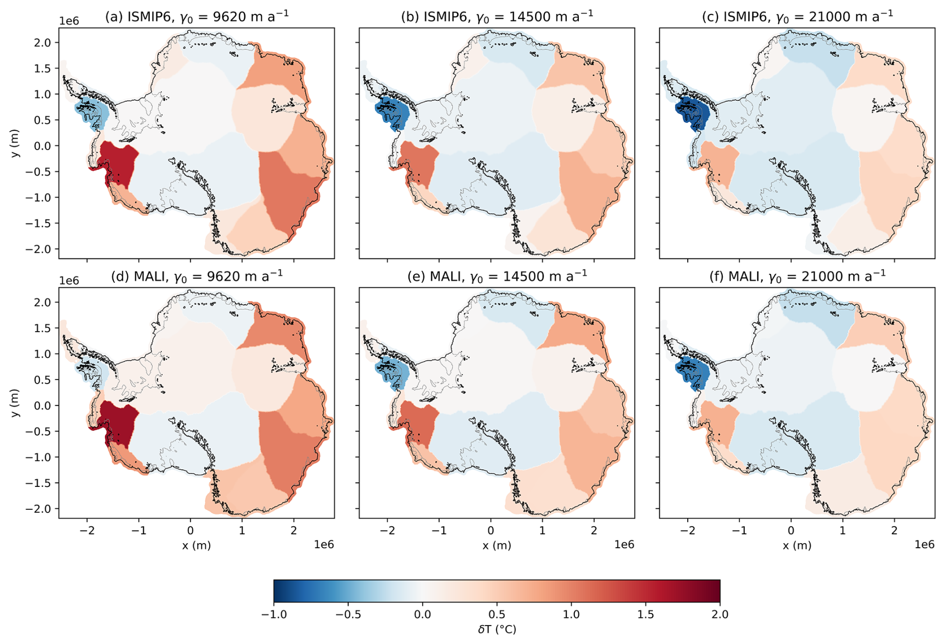
Figure B2 Temperature correction to ocean thermal forcing provided by ISMIP6 (a–c) and used in MALI simulations (d–f) for the three different values of the sub-shelf melt parameter, γ₀.

Appendix C: Control simulations

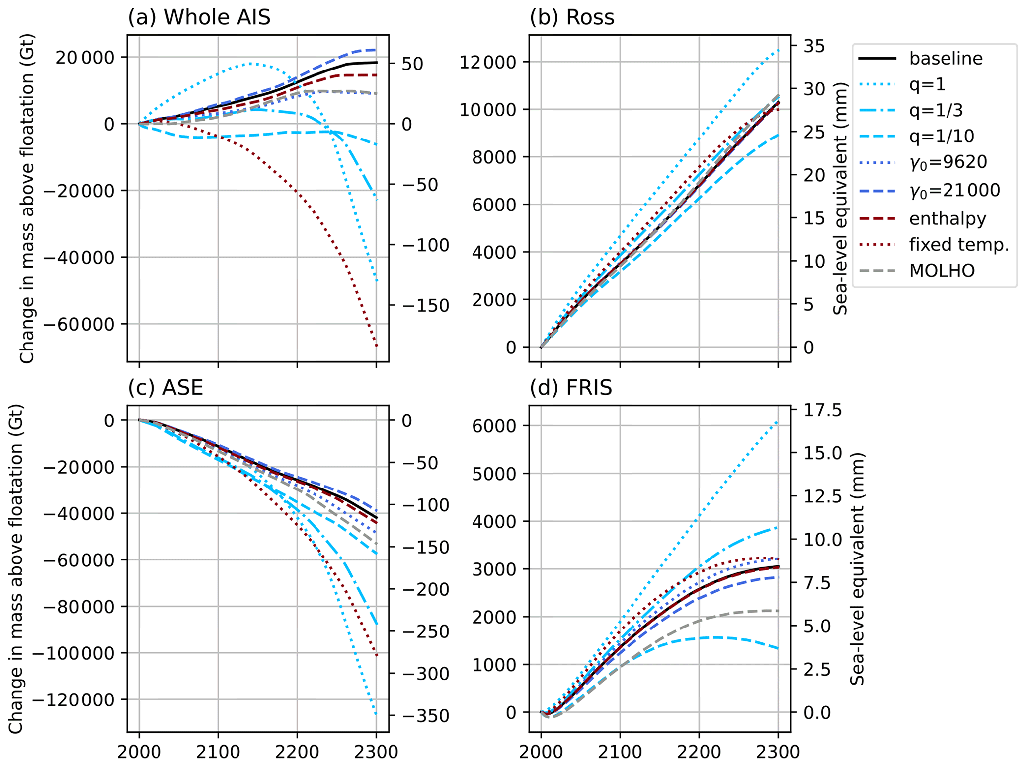
Figure C1 Mass change for the whole ice sheet (a) and regions of interest (b–d) from control simulations for the parameter and model fidelity sensitivity studies.

Appendix D: Full AIS sensitivity test maps

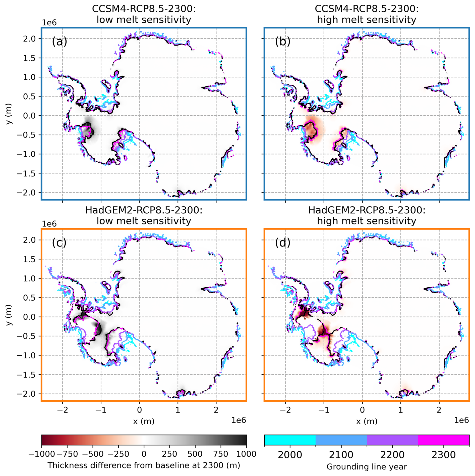
Figure D1 Maps of thickness relative to baseline runs (γ₀= 14 500 m a⁻¹) at 2300 for low melt sensitivity (γ₀= 9620 m a⁻¹) (a, c) and high melt sensitivity (γ₀= 21 000 m a⁻¹) (b, d) experiments. Grounding lines from the sensitivity experiments are shown by colored curves at 2000, 2100, 2200, and 2300, while the grounding lines at 2300 from baseline simulations are shown in black.

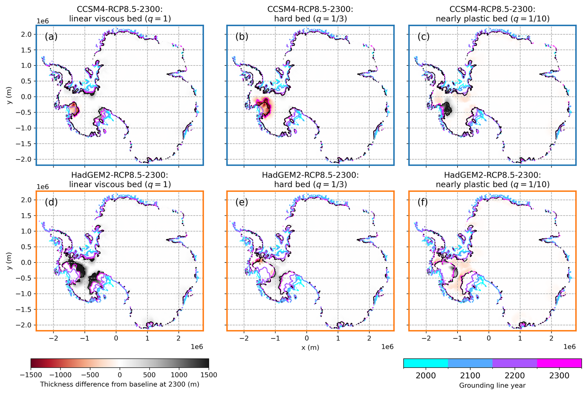
Figure D2 Maps of thickness relative to baseline runs ($q=\mathrm{1}/\mathrm{5}$) at 2300 for experiments with q values of 1 (a, d), $\mathrm{1}/\mathrm{3}$ (b, e), and $\mathrm{1}/\mathrm{10}$ (c, f). Grounding lines from the sensitivity experiments are shown by colored curves at 2000, 2100, 2200, and 2300, while the grounding lines at 2300 from baseline simulations are shown in black.

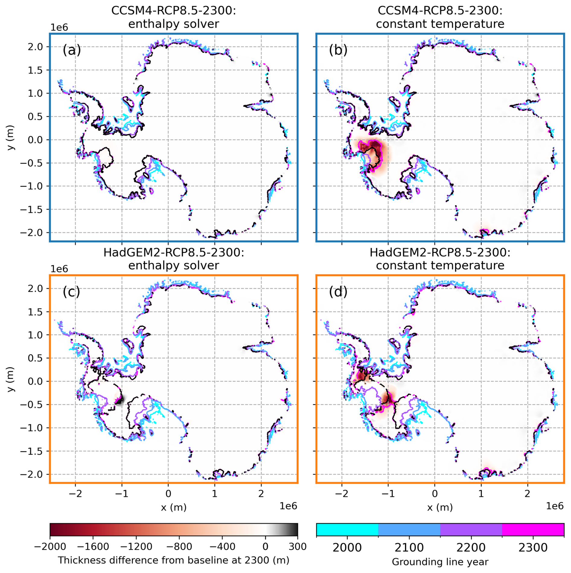
Figure D3 Maps of thickness relative to the baseline runs using the temperature formulation at 2300, for experiments using the enthalpy formulation (a, c) and a fixed temperature field (b, d). Grounding lines from the sensitivity experiments are shown by colored curves at 2000, 2100, 2200, and 2300, while the grounding lines at 2300 from baseline simulations are shown in black.

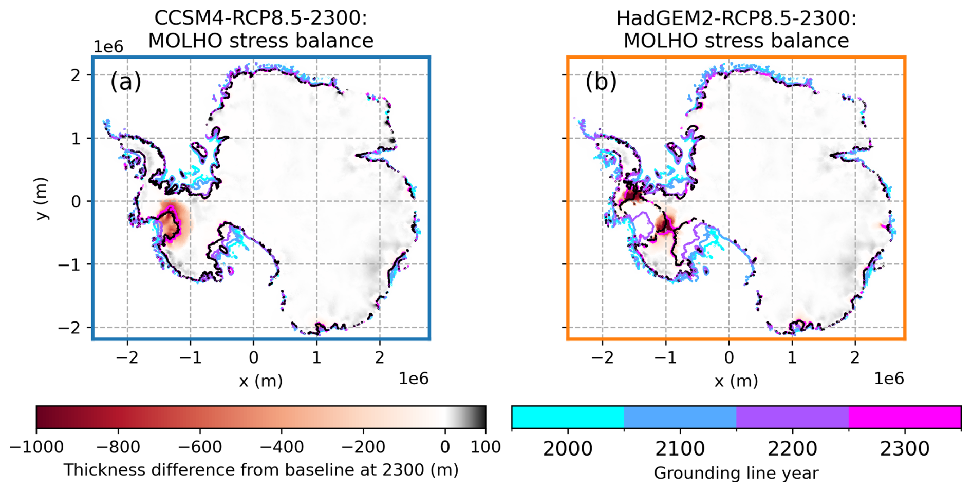
Figure D4 Maps of thickness relative to the baseline runs at 2300, for experiments using the depth-integrated solver. Grounding lines from the sensitivity experiments are shown by colored curves at 2000, 2100, 2200, and 2300, while the grounding lines at 2300 from baseline simulations are shown in black.