Winter Arctic polynyas in CMIP6 models

Winter Arctic polynyas, openings in the pack ice, play a crucial role for the climate from sea ice production to cloud formation and are hotspots for the ecosystem and human activity. Their area has significantly increased since satellite records began. Yet their representation has yet to be evaluated in any generation of global climate models, most likely because their automatic multi-model retrieval is challenging. We here use a newly-developed machine-learning based method and evaluate polynya activity against the satellite-derived one over 1979–2024 in the 18 CMIP6 models with daily sea ice concentration available. We find that models overestimate winter Arctic polynya area but underestimate its frequency, and limit their opening to the seasonally ice-covered regions. Polynya area is increasing in most models, but the bias of these trends are inconsistent. Although the model with the highest resolution has both the highest areas and frequencies, the sea ice model component is a more robust predictor of polynya activity, with most activity in the models whose thermodynamics scheme enhances ice growth/melt. Accordingly, we found more polynyas in the models with a larger seasonal cycle, in particular those with a warmer autumn that would delay ice growth or melt early. Finally, we confirm preliminary findings that polynya activity does not seem to impact the representation of the water column; if anything, we find less-dense water at the bottom of the continental shelf following larger polynya activity. Overall, our results suggest that in the Arctic, CMIP6 models unrealistically open only sensible-heat polynyas.

1 Introduction

Polynyas, non-linear openings enclosed in sea ice (World Meteorological Organization, 2014), are crucial for the climate, ecosystem, and the exploitation of polar regions. Winter polynyas expose the comparatively warm ocean to the frigid atmosphere, acting as “ice factories” (Smith and Barber, 2007) responsible for a non-negligible part of the total sea ice production in the Arctic (Preußer et al., 2019). The intense air-sea interaction also induces a strong heat- and moisture loss to the atmosphere (Morales Maqueda et al., 2004; Zhou et al., 2023) that results in cloud formation locally (Monroe et al., 2021) and even impacts the large-scale atmospheric circulation (Gordon et al., 2007). Sea ice production results in brine rejection at the surface of the ocean; in the Arctic, the dense water thus produced overflows off the shelf, modifying and ventilating the deep ocean (Aagaard et al., 1981; Martin and Cavalieri, 1989; Ohshima et al., 2016; Vivier et al., 2024). The combined effect of ocean mixing and air-sea exchanges further leads to intense gas exchanges and nutrient upwelling, making polynyas hotspots for marine life (Moore et al., 2023), which indigenous communities and whalers have long known and utilised (Hastrup et al., 2018).

Most Arctic polynyas are so-called “latent heat polynyas” that open in response to strong winds (Smith and Barber, 2007), often after a pre-conditioning period with warm air temperatures that thin the ice (Wong et al., 2026). They also open primarily on the continental shelf, close to the shelf break (Morales Maqueda et al., 2004). Winter Arctic polynya areas have been increasing since satellite record began in the 1970s (Wong et al., 2026), which is to be expected as the Arctic warms (Rantanen et al., 2022). However, the increase in polynya area appears to have slowed down over the last decade (Preußer et al., 2019; Wong et al., 2026), which Wong et al. (2026) explain as the result of inconsistent trends in winds in the Arctic, in particular their direction. It may also be that as polynyas grow and reach the shelf break, the oceanic forcing can no longer be ignored, and the mechanisms leading to polynya openings are changing (Morales Maqueda et al., 2004); Wong et al. (2026) did find that half of the Arctic regions had become hybrid polynyas, where thermodynamics also plays a role. Owing to the crucial role polynyas play in the climate system, understanding and projecting their changes is urgent. Before we can study future modelled polynyas, one needs to know how well historical polynyas are represented in climate models.

The latest generation of state-of-the-art global climate models are those who participated in the Climate Model Intercomparison Project phase 6 or “CMIP6” (Eyring et al., 2016). Their representation of the Arctic sea ice is acceptable but suffers many biases (Notz and SIMIP Community, 2020); it is common for authors to have to reject a large number of CMIP6 models whose sea ice concentration (Heuzé and Jahn, 2024) or thickness (Athanase et al., 2025) is unrealistic. Besides, both modelled Arctic air temperature (Tian et al., 2024) and wind speed (Zapponini and Goessling, 2024) are biased, and so is the upper Arctic Ocean (Muilwijk et al., 2023). We therefore expect the modelled Arctic polynyas to be biased as well. Besides, in the Southern Ocean, Mohrmann et al. (2021) and more recently Landrum et al. (2026) found large biases in the area and frequency of open water and coastal polynyas in CMIP6 models. To the best of our knowledge, nobody has assessed Arctic polynyas, in any CMIP phase, aside from an appendix figure showing the polynya frequency on the Siberian shelf in Heuzé et al. (2023), to try and explain biases in modelled deep Arctic Ocean properties in CMIP6. This is probably because Arctic polynyas are particularly tedious to detect in a multi-model framework, owing to the models' different grid geometries, resolutions and therefore representations of the coastline and archipelagos, and their treatments of the North Pole. Recently, Heuzé and Wong (2025) presented a new machine-learning based algorithm specifically designed to address these challenges, thus facilitating the detection of polynyas across different sea-ice models; we use their algorithm in this study.

Here, we evaluate the representation of winter Arctic polynyas in CMIP6 models. We quantify their biases in area, frequency and trends when compared to observations in Sect. 3, including the effect of using monthly output instead of daily output in Sect. 3.2. We then try to determine the causes for these biases in Sect. 4, looking at sea ice thickness, discussing the sea ice model components used, before moving to winds and air temperature. Finally, in Sect. 5, we go back to Heuzé et al. (2023) and the question that originally motivated this paper: do modelled Arctic polynyas impact the modelled deep Arctic Ocean?

2 Data and Methods

2.1 Polynya detection and observational polynya masks

We here use the new polynya detection algorithm of Heuzé and Wong (2025), developed with the explicit purpose to detect polynyas in CMIP6 models. As reviewed by e.g. Landrum et al. (2026) for the Southern Ocean and Wong et al. (2026) for the Arctic, there is no consensus in the literature regarding the sea ice concentration or thickness threshold that should be used to detect a polynya, be it for observations or models. Besides, prior to applying that threshold one has to perform a flood-fill to separate polynyas and open ocean (e.g. Mohrmann et al., 2021; Wong et al., 2026). Flood-fill algorithms change adjacent values to a common value, starting from a “seed” point in the open ocean, effectively detecting the ice edge. This is near-impossible to implement in a multi-model comparison framework in the Arctic owing to the models' different grids, in particular their treatment of the North Pole, their choice of reference longitude, and how their resolution represents the Canadian archipelago. Heuzé and Wong (2025) therefore took a new approach and developed, on observations and for CMIP6 models, a neural network-based method that detects patterns, gradients in the sea ice rather than absolute concentration or thickness values, and requires no flood-fill.

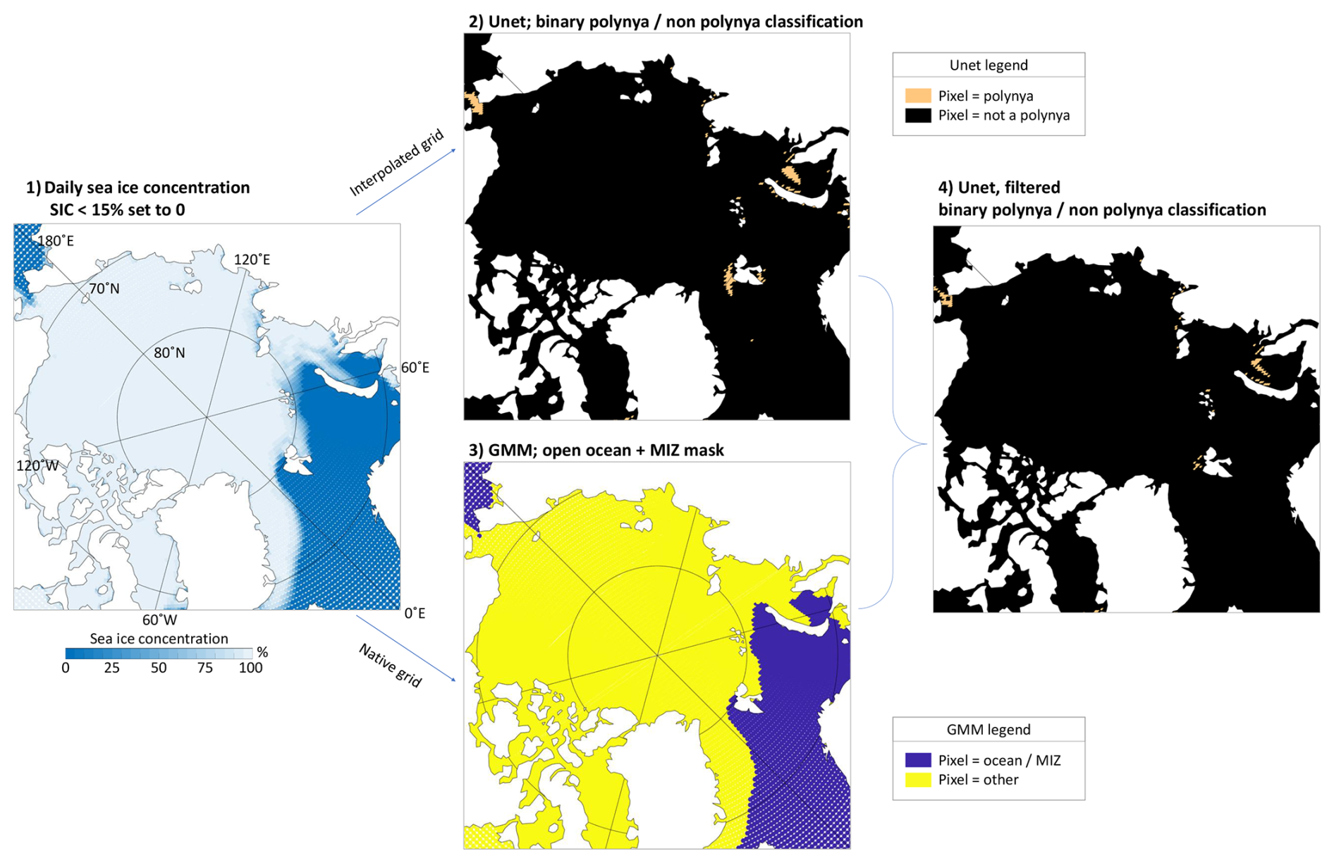
Figure 1 Steps of the polynya detection method, illustrated using the CMIP6 model MRI-ESM2-0 on 1 January 2015.

We now briefly describe how the algorithm works and re-direct the interested reader to the full publication (Heuzé and Wong, 2025) for the details. As summarised on Fig. 1, the method consists of four steps:

1. The daily sea ice concentration (SIC) input image is prepared: All pixels with SIC lower than 15 % are set to 0 to increase the sharpness of the ice edge, and all pixels south of 68° N are cut out. A second version is created by interpolating onto the National Snow and Ice Data Center (NSIDC) Northern Hemisphere Equal-Area Scalable Earth Grid 2.0 (Brodzik et al., 2012).

2. The interpolated daily SIC are passed through the “Unet” system, i.e. two convolutional neural networks that “zoom in” and “zoom back out” of the image, respectively, so that the result is a pixel-wise classification. Unet is particularly well suited to so-called anomaly detection (Ronneberger et al., 2015), in our case a small opening in the pack ice. The Unet system used here was trained by Heuzé and Wong (2025) using the daily NSIDC observational sea ice concentration as input (more information after this list) and the labelled daily polynya masks of Wong et al. (2026), which used a SIC threshold of 50 %, as target. As the model is already trained, this step takes barely a few seconds per model in our current study.

3. The sea ice on the native grid is passed through a Gaussian Mixture Model (GMM) system, an unsupervised classification method that Heuzé and Wong (2025) optimised to detect the open ocean and marginal ice zone (MIZ) pixels as one class. As the model is not trained, this step takes more than 1 h per model and ensemble member. Note that the output of the AWI-CM-1-1-MR CMIP6 model was too heavy on the native grid, so we had to use its interpolated version (the one used for step 2).

4. The GMM mask is interpolated onto the same grid as the Unet result to produce a filtered version of the Unet polynya/non polynya classification. Only pixels that are detected as polynyas in step 2 and not detected as open ocean + MIZ in step 3 are kept as polynya pixels in this step.

We leave the settings of Heuzé and Wong (2025) unchanged for Unet. For the GMM filtering, following their recommendation, we treat the input of step 3 differently for the observations and the CMIP6 models: For the observations, all daily sea ice concentration values lower than 40 % were set to 0; for the CMIP6 models, all values lower than 15 %. We tested also a 30 % threshold for CMIP6 but found no significant difference in the performance; since running the GMM on all models took nearly two weeks, we did not test other thresholds.

The observed daily NSIDC sea ice concentration from 1 December to 31 March, from 1978 to 2024, at a 25 km resolution, has already been classified at the pixel level as polynya/non polynya by Heuzé and Wong (2025). Rather than re-classifying the sea ice data, we here re-use the observed polynya masks of Heuzé and Wong (2025) as reference. The NSIDC sea ice concentration is retrieved from passive microwave satellites, processed with the NASA Team algorithm (Cavalieri et al., 1999). For Sect. 3.2 we generated a monthly observational reference by first computing the monthly mean of the NSIDC sea ice concentration from their daily data, and then passing these monthly sea ice concentration through the Unet + GMM algorithm.

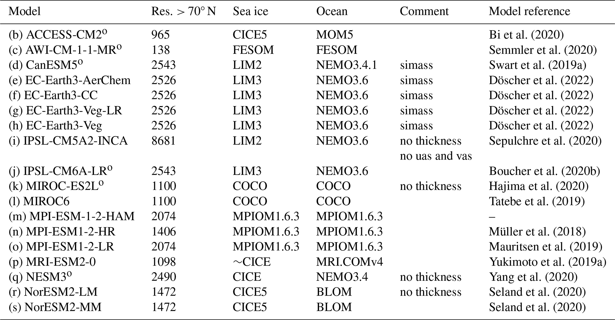
Bi et al. (2020)Semmler et al. (2020)Swart et al. (2019a)Döscher et al. (2022)Döscher et al. (2022)Döscher et al. (2022)Döscher et al. (2022)Sepulchre et al. (2020)Boucher et al. (2020b)Hajima et al. (2020)Tatebe et al. (2019)Müller et al. (2018)Mauritsen et al. (2019)Yukimoto et al. (2019a)Yang et al. (2020)Seland et al. (2020)Seland et al. (2020)

Table 1 For the models with daily sea ice concentration output: Model name and letter used on all figures and tables; Horizontal resolution “Res.” north of 70° N as grid cell area in km² (total area north of 70° N, in km², divided by number of grid cells north of 70° N); Sea ice component and version, when indicated in the reference (∼ means similar to, according to the reference); Ocean component and version, when indicated in the reference; Comments; and reference of the model description paper. ^o next to the model name indicates a model used in the ocean analysis of Sect. 5. See also Appendix Table A1 for the ensemble members, simulations, and dataset DOIs.

2.2 CMIP6 data: ice, wind, and ocean

To compare models to the full observational time series (1978–2024), we use both the historical run (Eyring et al., 2016) that finishes on 31 December 2014 and the Shared Socio-economic Pathway “SSP” climate change run (Tebaldi et al., 2021) of the Climate Model Intercomparison Project phase 6. Our analysis centres on the 18 models from 10 different model families that had daily sea ice concentration “siconc” available at the time of download (summer 2025), listed in Table 1. They cover nearly three orders of magnitude in horizontal resolution in the Arctic, from just above 100 km² per grid cell area for AWI-CM-1-1-MR to nearly 10 000 km² for IPSL-CM5A2-INCA. Most models are of the order of 1000 to 2000 km², or about 1° longitude/latitude. Their sea ice and ocean components will be further discussed in the analysis. We acknowledge that real-world Arctic polynyas are preferably detected using sea ice thickness rather than concentration (e.g. Tamura and Ohshima, 2011; Preußer et al., 2019). However, the daily sea ice thickness in CMIP6 is often not available, and it has been reported to have large errors compared to observations on multiple occasions (Mohrmann et al., 2021; Athanase et al., 2025), so we use the more reliable and widely available daily sea ice concentration. We also use the monthly sea ice concentration for a brief comparison; see Appendix Table A2 for the ensemble members and SSPs.

When possible, we used up to 10 ensemble members per model. The ensemble spread is the first thing analysed in Sect. 3. We tried to use only SSP2.4-5 but it was not available for some models. In the absence thereof, we used SSP3.7-0, and SSP5-8.5 when it was the only one available; see Appendix Table A1. As shown in Tebaldi et al. (2021), using different SSPs should have no impact on our results as the scenarios do not diverge before approximately year 2050 whereas we stop in 2024. We nonetheless redid the analyses with the historical run only and find no significant difference (not shown): the values were obviously different, but the correlation between the two was near-perfect, and most importantly, the relative model biases were unchanged.

For investigating the potential causes of polynya biases, we use the monthly sea ice thickness “sivol” (in m, computed as the total volume of sea ice in m³ divided by grid-cell area in m²) since the daily thickness has large errors, as we described above, or is not available. Note that the variable “sithick” exists but is ambiguously defined as the floe thickness, and is less widely available than “sivol”. For CanESM5 and the EC-Earth3 models, “sivol” is not available; we used “simass” (total mass of sea ice divided by grid-cell area) that we converted to sivol by dividing it by their ice density of 917 kg m⁻³ (Vancoppenolle et al., 2023). Because of missing files, only 14 models can be used for this analysis; the other four are marked with “no thickness” in Table 1. We also used the daily surface zonal and meridional wind speeds “uas” and “vas”, respectively; they were not available for IPSL-CM5A2-INCA, as indicated in Table 1.

For investigating potential consequences of polynya activity on the ocean, we used the monthly full-depth potential temperature “thetao” and practical salinity “so” on the models' native grid. Full depth variables being very heavy, we use only the three models with the most and three models with the least polynya activity (^o next to the model name in Table 1). As we will show, there is a large agreement in polynya activity across ensemble members, so we use only the first ensemble member of each model: r1i1p1f1 for ACCESS-CM2, AWI-CM-1-1-MR, CanESM5, IPSL-CM6A-LR, and NESM3, and r1i1p1f2 for MIROC-ES2L.

2.3 Polynya statistics and other analyses

In line with e.g. the “real” Arctic polynya assessment of Preußer et al. (2019) or that of polynyas in CMIP6 in Southern Ocean of Mohrmann et al. (2021), our evaluation metric is the yearly/winter mean polynya area. We define winter for polynyas as the period from 1 December to 31 March to reduce the risk of mis-detecting late freeze-up and early melt onset as polynyas. The yearly/winter mean polynya area is then the mean of the daily polynya areas, which are for each day the sum of the grid cell areas of all pixels detected as a polynya. For some diagnostics, we keep the 45-winter time series. For most of the manuscript however, we then compute the 45-winter mean of the mean polynya area. We tested using instead the historical run only (i.e. 1979 to 2014 instead of 1979 to 2024) and found no significant differences, with correlations exceeding 0.99 (not shown); we found the same result if using instead 1982–2014 as Tian et al. (2024) did.

Two other diagnostics were used by Wong et al. (2026): the cumulative polynya area, i.e. sum of the daily values instead of the mean (described above), and the total area of each winter, i.e. the sum of the grid cell areas of all pixels detected as a polynya at least once each winter. We computed them both for all CMIP6 models (not shown) and found a near-perfect correlation (> 0.9) between our yearly/winter means and their diagnostics. In particular, the relative biases of the models did not change, i.e. the models with the largest values with one diagnostic were still the largest with another one. We therefore use the yearly mean polynya area only. We define the polynya frequency of each pixel as the number of winters where that pixel is detected as a polynya at least once.

As is common in observational studies (e.g. Tamura and Ohshima, 2011; Preußer et al., 2019; Wong et al., 2026), we study the polynya behaviour of different regions of the Arctic separately. We use the same region definition as Wong et al. (2026) as it is optimised to reduce noise from incorrectly detected marginal ice zone and is adapted to the same time period as our study, including the emergence of polynyas in north-east Greenland. The coordinates of each region are given in Appendix Table A3 and shown on the first pan-Arctic map of Sect. 3.

Unless stated otherwise, all across-model correlations shown are significant at 95 % and conducted on the ensemble-average values. We show linear regressions only if the corresponding regression is significant. For the trend analysis, linear trends (with 95 % significance) are calculated on the individual ensemble members first and the ensemble-average trend is the value presented. As for the yearly means, changing the time period for the trend calculation to 1979–2014 or even 1982–2014 made no significant difference (not shown), and in particular did not change the models' relative biases.

For the beginning of the analysis, where we determine the pan-Arctic behaviour of the models, the sea ice area is computed as the sum of all concentration x grid cell area, using the concentration on the interpolated grid cut at 68° N. Using the same grid, the sea ice extent is computed as the sum of the grid cell areas for all grid cells where the concentration is strictly larger than 15 %. Along with the 1979–2024 mean of the whole-year means we also compute the mean seasonal cycle: for each year, we compute the difference between the yearly maximum and the yearly minimum SIA or SIE, respectively, and take the 45-year mean.

The objective of this study is to try and find a link between polynya biases and model biases across the CMIP6 ensemble, not to conduct a process study in individual models. Therefore, our priority is to find across-model relationships. Only in the absence of such relationship do we resort to time series correlations at the individual model level. Since polynya area and frequency have regularly been linked to wind speed, including its extremes, and air temperature (see Wong et al., 2026, and references therein), we use these two parameters in our study.

The daily wind speed is computed from the daily “uas” and “vas”. In each region, we extract the mean of the three variables, but also their 90th percentile as the most extreme value. For the two components of the wind “uas” and “vas”, we have to extract both the 10th percentile (most extreme negative values, i.e. west- or southward) and the 90th percentile (most extreme positive values, i.e. east- or northward).

We use the air temperature biases of Tian et al. (2024). They use only the first ensemble member of each model (r1i1p1f^∗), only the time period 1982–2014 (historical run), and before computation regridded all the models to a common 1° grid. For across-model correlations, we therefore also use the first ensemble member only and the 1982–2014 time period for our polynya areas. Compared to our list of models, the only model missing from their study is AWI-CM-1-1-MR. All their values are biases, i.e. model value minus a common satellite-based reference; see Tian et al. (2024) for more information. Since it is a common offset for all models, it has no impact on our across-model correlations.

Finally for the ocean variables, we limit our investigation to a comparison of the Kara and Laptev seas. We extend the geographical limit of the Kara Sea northward to 86° N compared to the rest of the study (coordinates in Appendix Table A3) to capture the potential effect of the polynya not only on the water column below, but in the deep basin offshore via potential dense water overflows and effects on the halocline; the original definition of the Laptev Sea already includes the relevant deep ocean area. We further split each sea into three regions based on their bathymetry

• continental shelf: shallower than 500 m;

• shelf break: bathymetry between 500 and 1000 m;

• abyssal plain: deeper than 3000 m.

The bathymetry itself was computed as the depth of the last level with salinity data, since the modelled bathymetry “deptho” was not available for all models at the time of download. We compute the bottom properties as the properties T and S in that last level. Given the large range of depths considered, we use the density anomaly referred to 2000 m σ₂, computed following TEOS10 as implemented in the Gibbs SeaWater toolbox (Roquet et al., 2015). Finally, following Heuzé et al. (2023), we extract each model's properties of the Atlantic Water core, defined as the depth of the maximum temperature deeper than 200 m.

3 Results: Assessment of biases in winter Arctic polynya

3.1 Polynyas are too large but do not open often enough

At the pan-Arctic scale, 10 out of 18 models overestimate the winter polynya area for all their ensemble members (Fig. 2). The largest overestimation is from AWI-CM1-1-MR, which is nearly 10 times too high. This is also the model with the highest horizontal resolution by far (Table 1), which is consistent with both Wong et al. (2026) and Landrum et al. (2026) who showed that higher resolution in the product leads to larger polynya area detected. The bias does not seem related to the ocean model: both CanESM5 and NESM3 use the same model NEMO (both version NEMO3.4), yet the polynya area in CanESM5 is twice as large as the observations, while that of NESM3 is only a third of the observed area. We will show in Sect. 4.1 that this is probably a consequence of their different sea ice models. The intermodel spread is much larger than the spread across ensemble members of each model (Fig. 2). This result still holds when looking at the individual regions separately (Appendix Fig. ). The rest of the bias analysis is therefore done with the ensemble mean of each model, unless specified otherwise.

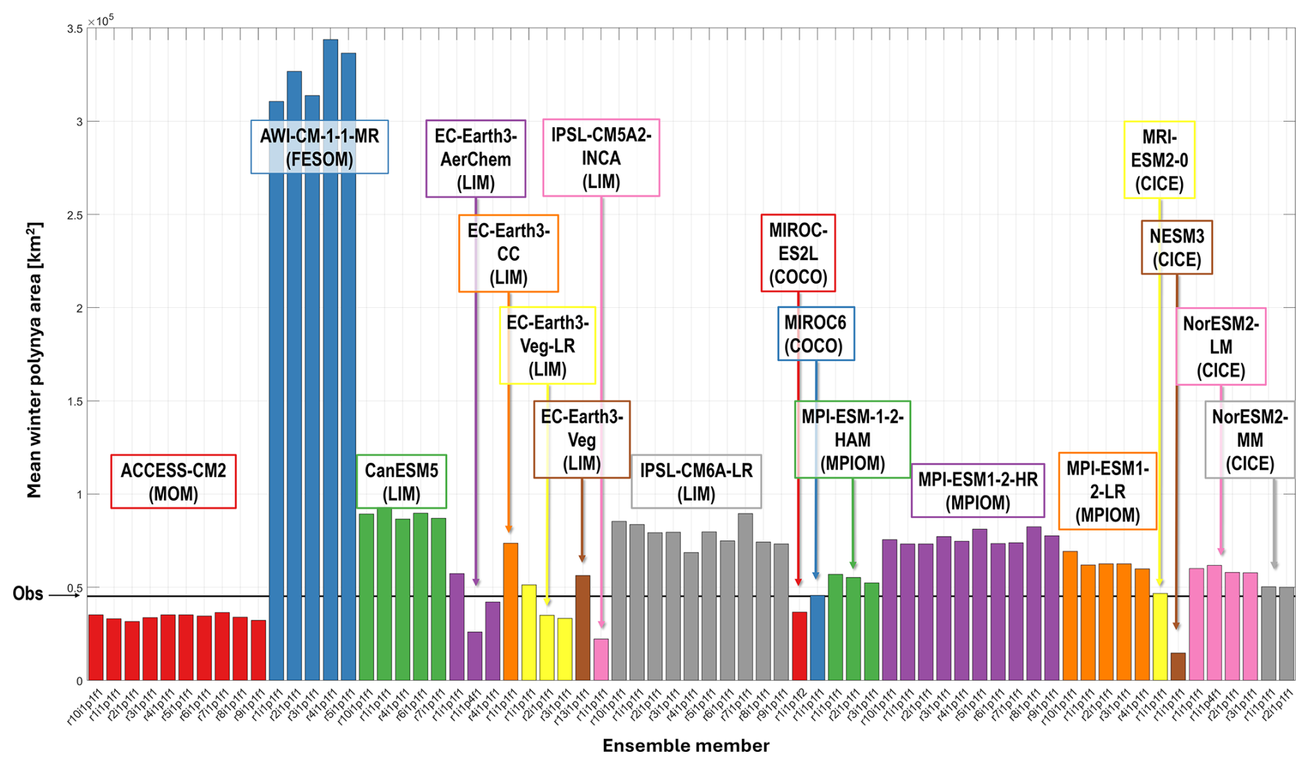
Figure 2 1979–2024 mean of the winter (December–March) mean polynya area for the entire Arctic, for the observations (black horizontal line) and for each ensemble member of the models with daily sea ice concentration. Individual regions shown on Appendix Fig. . Acronym in parentheses is the sea ice model family, as discussed in the rest of this section and in Sect. 4.1.

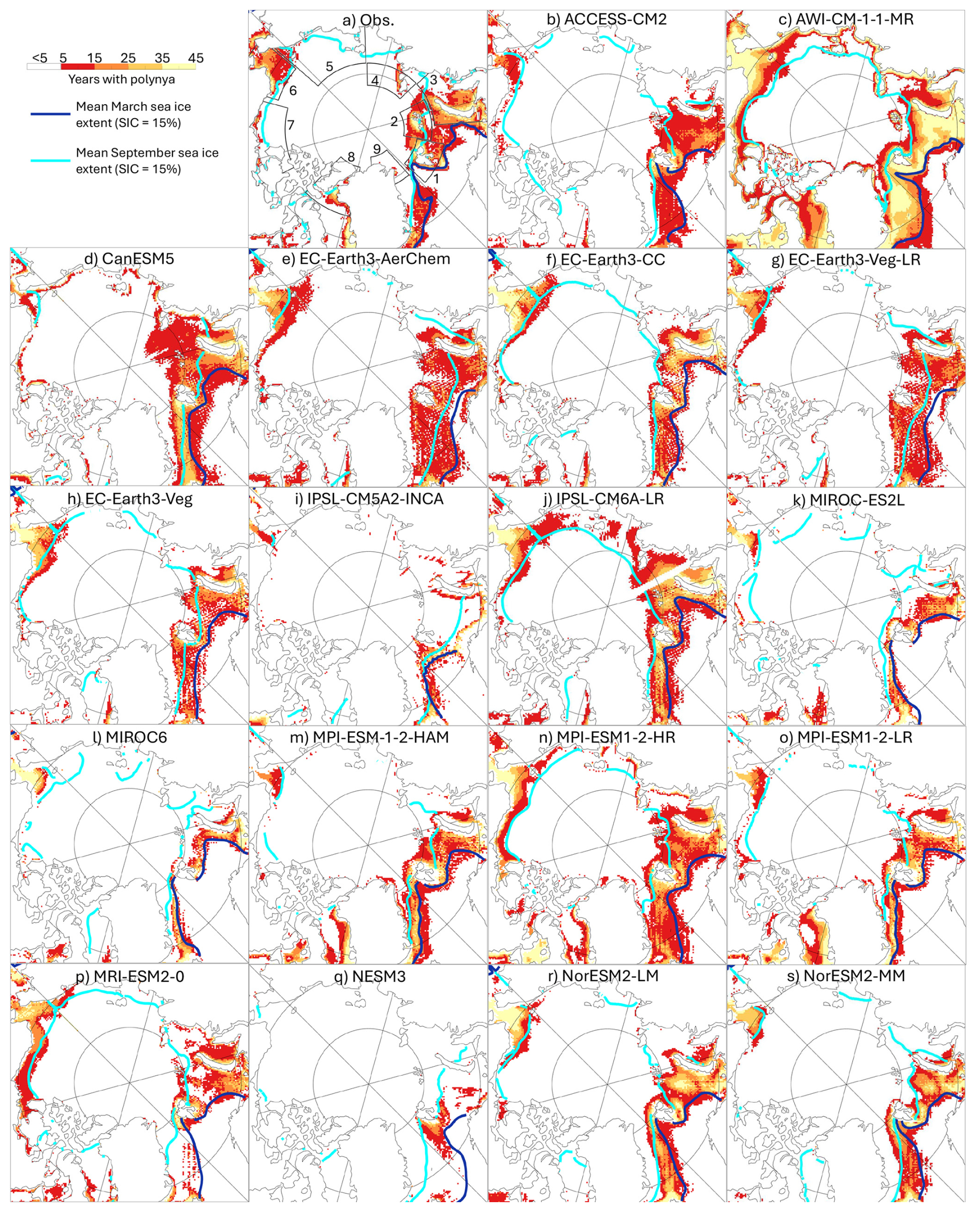
Figure 3 For each pixel, for the observations (a) and the ensemble-average of the CMIP6 models with daily output, number of winters over 1979–2024 where a polynya opened there at least once between 1 December and 31 March. Note that polynyas are detected using sea ice concentration only. Dark blue and cyan are the mean sea ice extent in March and September, respectively, over the same period 1979–2024; the “tail” of sea ice (cyan line) in the top-left corner along 180°, seen for some models, is a plotting artefact. Thick black lines on (a) are the regions used in this study, as per Wong et al. (2026), also defined in Appendix Table A3.

At the pan-Arctic scale, models not only overestimate the 45-year mean polynya area, they also overestimate how often polynyas open (Fig. 3). Most models have more polynya activity than the observations, either because low-activity areas extend further north or south (red colours), or because the regions are more active than the observations (yellow colours). In observations, an increase in polynya activity as sea ice area/extent declines has been reported (e.g. Preußer et al., 2019; Heuzé and Wong, 2025; Wong et al., 2026). At the multi-model level, we find the opposite relationship. We find an across-model correlation between pan-Arctic sea ice area/extent and mean winter polynya area of 0.75/0.84, i.e. the models with most sea ice also have the most polynyas. This is most likely because, with the exception of CanESM5 and the EC-Earth3 models, polynya activity in models is mostly limited to the seasonally ice covered area (between the summer extent in cyan and the winter extent in dark blue, Fig. 3), whereas in observations there are polynyas in the inner ice pack (north of the cyan line). The across-model correlation between polynya activity and the model's mean seasonal cycle in SIA/SIE is 0.50/0.53: the larger the seasonally ice-covered region, the more polynyas. This suggests a link with sea ice thickness, which we will investigate in Sect. 4.

Again, the highest resolution model AWI-CM1-1-MR has the most activity. Note that we visually verified its daily sea ice concentration output and can confirm that these are indeed polynyas. There are however many pixels with a low polynya opening frequency out of the main, predefined regions, for most models: this is noise from the marginal ice zone in the North Atlantic, Barents Sea and on the Pacific side. As discussed both for observations by Preußer et al. (2016) and for models by Heuzé and Wong (2025), this is unavoidable in the Arctic, even with traditional threshold + flood-fill methods, owing to the complex shape of the coastline and the MIZ itself. To reduce this noise, we conduct the rest of the bias analysis on the nine regions highlighted on Fig. 3a (see also Appendix Table A3).

Table 2 For each region, percentage of the region where there is a polynya more than 25 out of 45 winters over 1979–2024, for the observations (top row) and the ensemble-average of the models. Only non-land pixels considered.

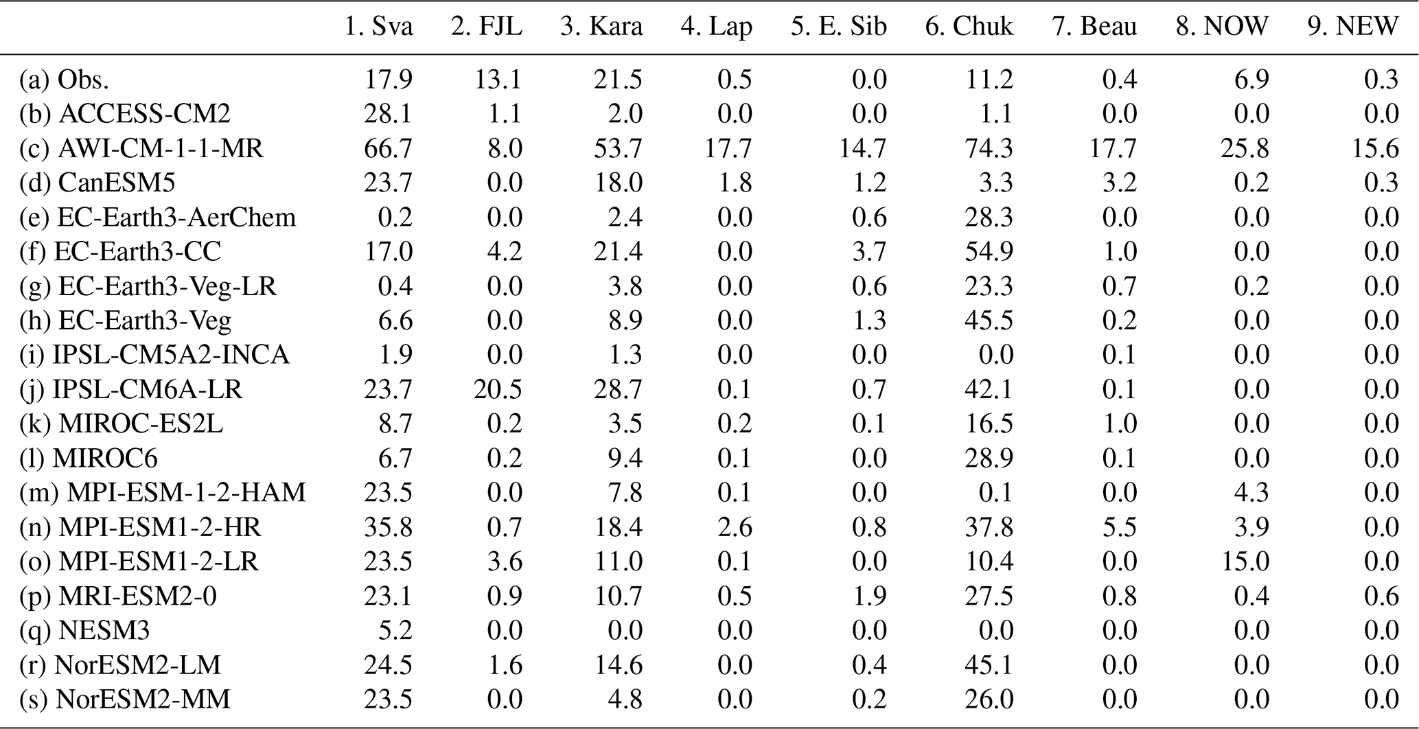
To quantify the biases in polynya frequency, we compare the percentage of each region where polynyas have opened for more than 25 out of the 45 years (not necessarily continously), in both models and observations (pale orange and pale yellow on Fig. 3). In the regions Svalbard (column 1 in Table 2), East Siberian (5) and Chukchi (6), a majority of models overestimate locations that have a high opening frequency (10, 12 and 12 models, respectively). The overestimation is most dramatic in the East Siberian Sea where the observational value is 0. Most models show very little activity in the North Water Polynya (NOW, column 8). This region is one of the most active polynya regions in the Arctic but is difficult to model owing to the narrow straits and complex bathymetry (e.g. Moore et al., 2023). It is therefore surprising that the models' behaviour in the North Water Polynya region is not related to the model's horizontal resolution. For example, the higher resolution MPI-ESM1-2-HR is lower than observations (3.9 % instead of 6.9 %, column 8 in Table 2), but its low resolution counterpart MPI-ESM1-2-LR is higher than the observations (15.0 % instead of 6.9 %).

The largest overestimation of the frequent-opening locations is from AWI-CM-1-1-MR in the Beaufort Sea, with a value 48 times that of the observations. In fact, this model largely overestimates the area with frequent polynyas in all regions except Franz Josef Land, where it underestimates it by nearly half (8.0 % instead of 13.1 %). MRI-ESM2-0 is the only other model that is quite consistent in overestimating the frequent-opening areas: it does so in all regions except Franz Josef Land, Kara Sea, and the North Water polynya. It is more common for CMIP6 models to underestimate the frequent-opening areas: seven of the models do so in at least 7 out 9 regions (ACCESS-CM2, EC-Earth3-AerChem, EC-Earth3-Veg, IPSL-CM5A2-INCA, MIROC6, MPI-ESM-1-2-HAM, NESM3), and 13 in at least 6 (same + EC-Earth3-CC, EC-Earth3-Veg-LR, MIROC-ES2L, MPI-ESM1-2-LR, NorESM2-LM, NorESM2-MM). In summary, even though Fig. 3 suggests that models open polynyas too often, what they do is to open with a low frequency at too many locations. The modelled polynyas' spatial distribution is mostly confined to the marginal seas and rarely form in the central ice pack.

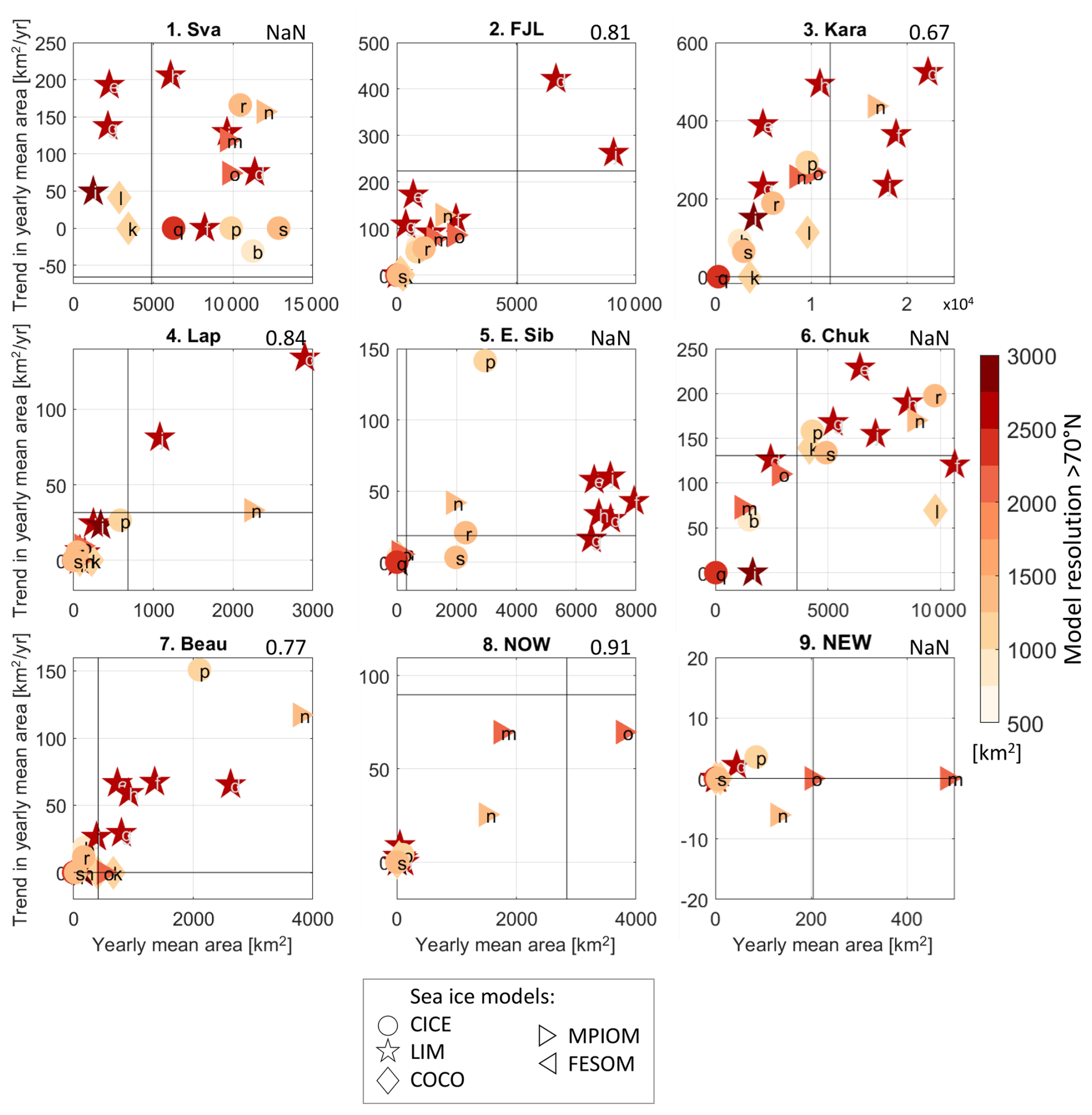
Figure 4 Across-model relationship between the 1979–2024 mean of the winter-mean polynya area (x-axis) and the 1979–2024 trend (95 % significance) in winter mean polynya area (y-axis) for each region as defined in Appendix Table A3. If the trend is insignificant, it is shown here as 0. Models referred to with same letters as on Fig. 3. Numbers in the top right corner of each panel is the correlation between the two (95 % significance), considering only the models with a significant trend; “NaN” means no significant correlation. Black lines are the observational values. Shading is each model's nominal resolution north of 70° N; symbol, its sea ice component. AWI-CM-1-1-HR is excluded for clarity; see Appendix Fig. A2 for the version with that model included. Mean area and trend values are also given in Appendix Table A4.

Finally, winter Arctic polynya area has been increasing in observations (e.g. Preußer et al., 2016, 2019; Wong et al., 2026), with Wong et al. (2026) in particular finding positive trends since satellite records began in all regions except Svalbard. Do the CMIP6 models reproduce these trends? In most regions, even in Svalbard, a majority of CMIP6 models exhibit a positive trend in polynya area over 1979–2024 (Fig. 4). The trend is however inaccurate when compared to the observed one, but there is no consistency in whether the models over- or underestimate it (compare symbols to the horizontal black line). We find rather that there often is a relationship between the 45-year mean bias in polynya area and the bias in trend of the polynya area (Fig. 4), with five regions exhibiting large significant positive correlations between the two, albeit with three different behaviours. In Franz Josef Land (region 2, R = 0.81) and the Laptev Sea (region 4, R = 0.84), most models have a low bias in both 45-year mean and trend, except for CanESM5 (d) and IPSL-CM6A-LR (j) that have a large bias in both. In the Kara (3,  0.67) and Beaufort (7,  0.77) seas, all models overestimate the trend, but the trend is greater for larger polynya areas. In the North Water polynya (8,  0.91) in contrast all models underestimate the trend, but likewise the trend is larger for larger polynya areas. Note that AWI-CM-1-1-MR is excluded, as it is a clear outlier; when it is included (see Appendix Fig. A2), all regions except the MIZ-dominated Svalbard have an extremely strong correlation, exceeding 0.9 in five regions. Note that although Heuzé and Wong (2025) found, in observations, an increased performance of the detection algorithm as SIA/SIE decreased, we find no across-model correlation between the trends in SIA/SIE and either the trend or mean values of the polynya area.

In summary, there is no across-model agreement on the polynya area trend, rather different clusterings in the different regions. We see no link with the model resolution in any of the regions (shading on Fig. 4), but there appears to be some clustering by sea ice model. The LIM models (stars on Fig. 4) in particular are often found together, most visibly by the Pacific inflow regions of the East Siberian (all of them are to the right) and Beaufort seas (all of them are to the bottom centre/left). We will investigate why that might be in Sect. 4, but first, since the number of models with daily sea ice is way less than that with monthly sea ice, let us investigate the impact of using monthly CMIP6 data for polynya detection.

3.2 A linear relationship between values from daily and monthly output

There are nearly twice as many CMIP6 models with monthly sea ice concentration than with daily sea ice concentration (35 vs 18). It is therefore tempting to try and detect polynyas in CMIP6 models using monthly data, although polynyas usually last but a few days (Smith and Barber, 2007). We can immediately see that both areas and frequency are largely underestimated when using monthly output (Fig. ), including for the monthly-version of the observations where only a handful of pixels have a polynya 5 to 10 out of the 45 years, but none more often than that (i.e. only red pixels on Fig. a). The same holds for the CMIP6 models, with most models having very few polynya pixels at the pan-Arctic scale, and nearly no model having frequencies exceeding 15 years (i.e. another colour than red) anywhere.

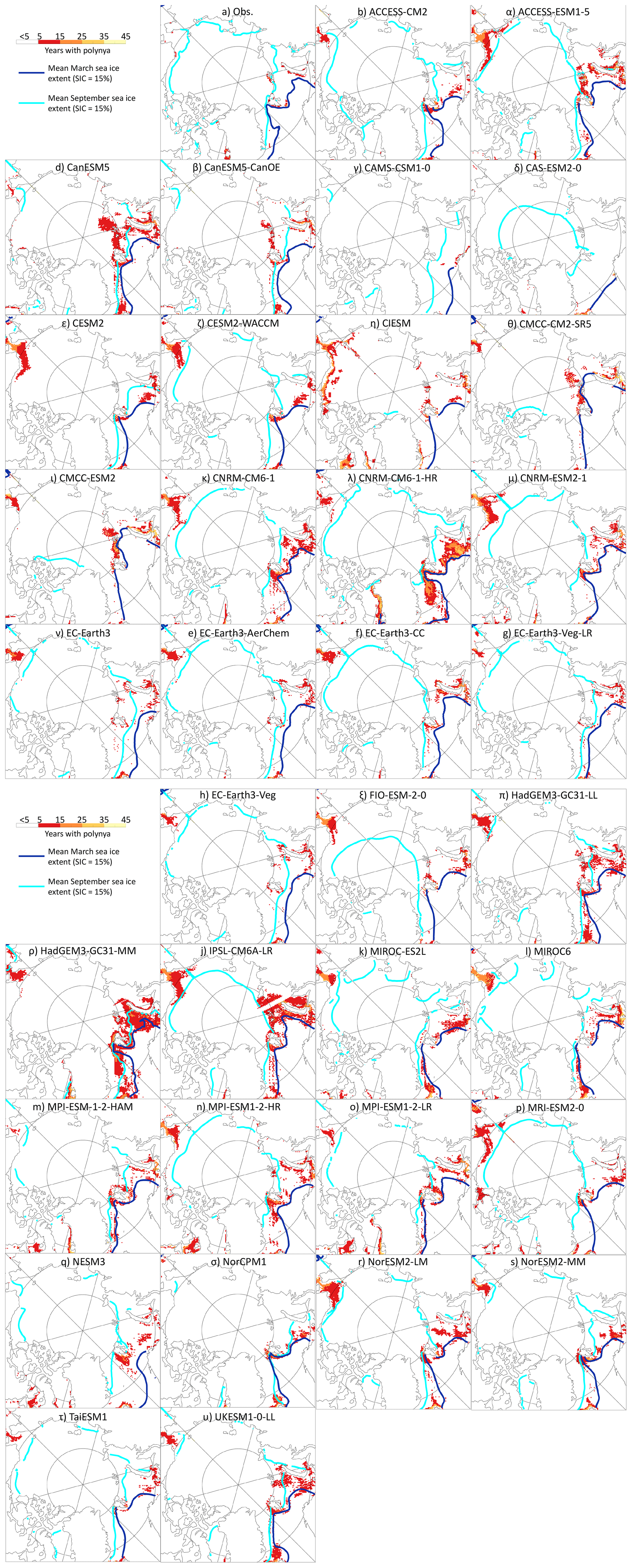
Figure 5 Same as Fig. 3 but for monthly output: For each pixel, for the observations (a) and the ensemble-average of the CMIP6 models with monthly sea ice output, number of winters over 1979–2024 where a polynya opened there at least once between 1 December and 31 March. Dark blue and cyan are the mean sea ice extent in March and September, respectively, over the same period 1979–2024; the “tail” of sea ice in the top-left corner of some models is a plotting artefact.

The relationship with the sea ice area/extent and its seasonal cycle have also been lost, probably because of the extreme behaviours in the monthly-only models. Without the need for any calculation, we can flag several models as having clearly inaccurate sea ice concentration, models that are therefore not trustworthy in terms of their polynya representation. For example, CIESM and the two CMCC models have virtually no summer sea ice on average over 1979–2024 (cyan contours around the Canadian archipelago on Fig. ). CAMS-CSM1-0, CAS-ESM2-0, and the CNRM models in contrast have an immense winter ice cover (dark blue contours), including the entire Greenland Sea all the way to Iceland. CAS-ESM2-0 also has one of the most extreme seasonal cycles (distance between the cyan and dark blue lines), while CESM2 has virtually none. Should the reader consider using monthly output for a polynya analysis, we strongly recommend that they reject these models with unrealistic sea ice cover.

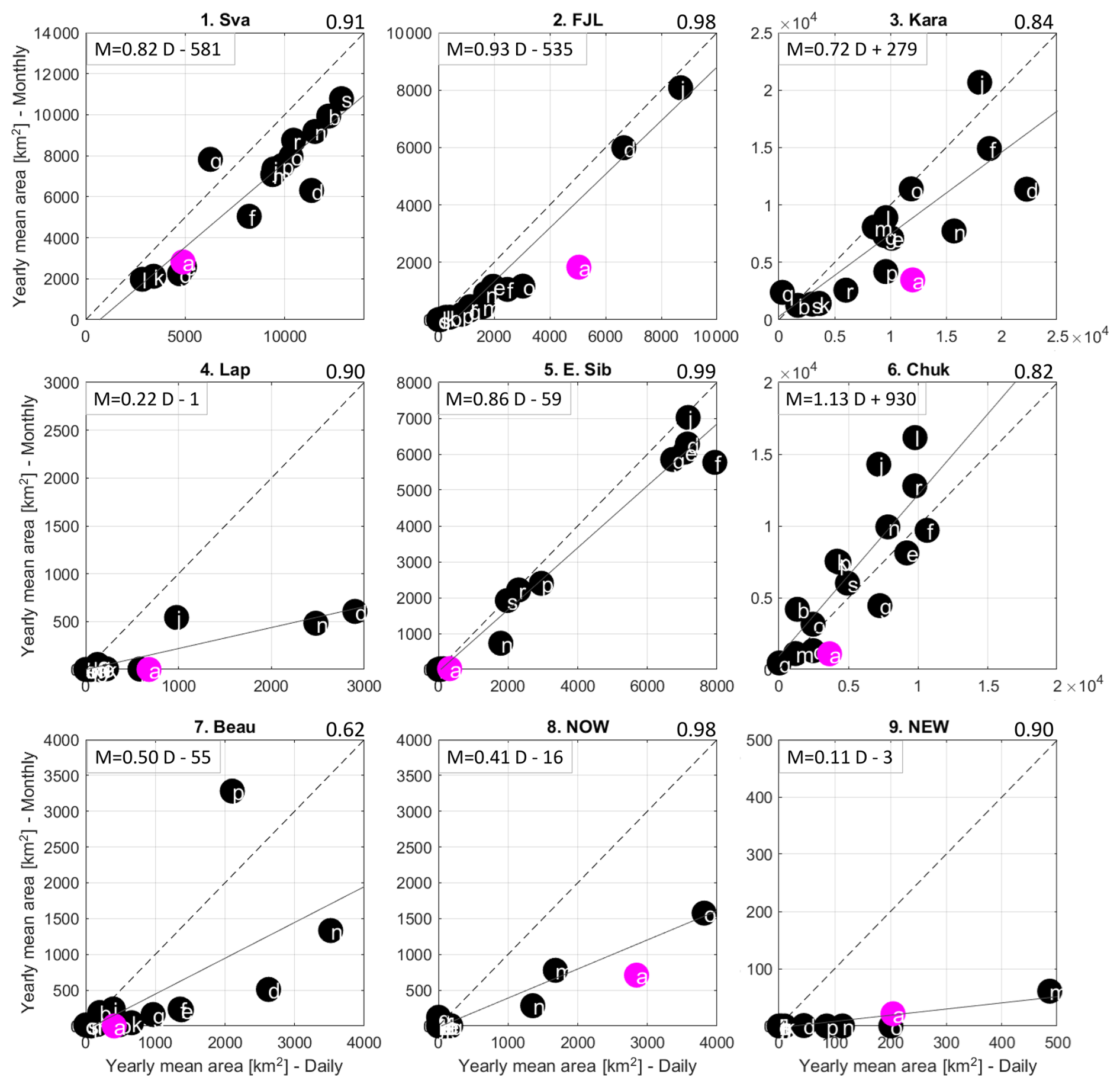
Figure 6 For the models that have both daily and monthly sea ice concentration, across-model relationship between the 1979–2024 mean of the winter mean polynya area computed from the daily output (x-axis) and that from the monthly output (y-axis) for each region as defined in Appendix Table A3. Models referred to with same letters as on Fig. 3. Numbers in the top right corner of each panel is the correlation between the two (95 % significance), considering only the models with a significant trend. Equation in the top left corner is the linear relationship between monthly “M” and daily “D” values, also shown as the plain black line. Dashed black line is the unit x=y line. Observational values shown as magenta dot but not included in the correlation or regression calculation.

AWI-CM-1-1-MR and IPSL-CM5A2-INCA are not available as monthly output, and EC-Earth3-Veg had no ensemble member in common for the daily and monthly output at the time of download. We therefore momentarily limit our study to the 15 remaining models and compare the mean polynya area obtained when using their daily or monthly output. Note that we used only the ensemble members common to both time resolutions, so the polynya area values presented on Fig. 6 differ slightly from those on Fig. 4 and in Appendix Table A4.

We find a very strong significant across-model correlation in all regions between polynya area from monthly and that from daily values (Fig. 6). In four regions, as expected, the monthly value is much smaller than daily: half as small in the Beaufort Sea (region 7), 0.4 times in the North Water polynya (region 8), 5 times smaller in the Laptev Sea (region 4), and up to 10 times smaller in the North East Water polynya (region 9). In four more regions, the regression shows a nearly one-to-one relationship between the monthly and daily results (0.82 in Svalbard, 0.93 in Franz Josef Land, 0.72 in the Kara Sea, and 0.86 in the East Siberian Sea). Because detection in these regions is impacted by noise from the MIZ, this agreement suggests that monthly and daily results are similarly impacted. In the Chukchi Sea (region 6), the monthly results are larger than the daily results for 6 of the models, which toggles the regression slope above 1. That is the only such region. Visual inspection (not shown) reveals that the daily sea ice there is very “binary” in these models: small areas are clearly open (concentration of 15 % or less) next to a very sharp transition to the consolidated ice pack (concentration above 80 %). So even though this transitional zone varies a lot from day to day, this results in a large region with sea ice concentration around 40 % as monthly mean, which the algorithm detects as a large polynya. The same happens to MRI-ESM2-0 (model p) in the Beaufort Gyre (not shown): It experiences a very late freeze up in December 2015 and 2017, during which the daily ice edge moves a lot from daily to daily images. The daily polynya area is not affected, since these regions are filtered out as open ocean for the daily results, but the resulting monthly mean sea ice concentration is low over a large region and erroneously interpreted as many polynya pixels for the monthly result.

Note that standard threshold methods would be affected by these behaviours as well, unless the authors select a high sea ice concentration as threshold, which then further reduces their ability to remove the marginal ice zone. This could be fixed in our method by fine-tuning the thresholds and settings of either Unet or the GMM per model and/or region, but we want to keep the same values for all models, at the pan-Arctic scale. One could also use the daily sea ice concentration to generate the MIZ filter and apply it to the monthly classification result, although the computing time saved would be unsignificant – if daily output are available, we recommend their consistent use. A dedicated study of these specific models in the Chukchi and Beaufort seas is beyond the scope of this paper. Note also that even though the observations are not included in these correlation and regression calculations, they fall close to the regression line but have systematically lower results from monthly than daily values, as is to be expected.

In summary, one can mix and match monthly and daily results if one is careful, since the relationship between the two differs depending on the Arctic region. We recommend against doing that and would rather encourage the widespread release of daily sea ice data, as polynyas are short-lived events that open and close on daily to sub-daily time scales. For that reason, in the next section, we use only the daily outputs. We would also like to re-iterate that sea ice concentration alone is not optimum for detecting polynyas in the Arctic and would welcome a widespread release of daily sea ice thickness output.

4 Potential causes of biases in winter Arctic polynyas

In this section, we highlight processes or features that might explain the biases in winter Arctic polynya activity in CMIP6 models. The reader must bear in mind that a proper mechanistic understanding is impossible as we do not have access to the high-resolution model output O(10 min), only their daily average. Likewise, we do not have access to the model code and cannot run sensitivity experiments, only point out similarities. Therefore this section relies only on correlations, at the individual model level and across-models, and carefully discusses potential causalities.

4.1 Sea ice thickness and sea ice model

One expects a negative correlation between sea ice thickness and polynya area in winter, since sea ice thickness is commonly used to detect polynyas Preußer et al. (e.g., 2016). For each model and each region, we correlate the time series of their region-average, season-average sea ice thickness with the time series of the same region's DJFM polynya area. We indeed find negative correlations between winter thickness and winter polynya area in most regions for most models (Appendix Table A5): the thinner the winter sea ice, the larger the polynyas that same winter. The occasional positive correlation in the Svalbard region in our opinion is an indirect one, which rather indicates that by definition where there is sea ice (an exception in that region, the norm in all the others), polynyas can open. We also find many significant negative correlations with the previous summer (JJA) and autumn (SON) ice thicknesses. However, since there is a strong autocorrelation between different seasonal sea ice thicknesses (around 0.5 in all regions and models, not shown), and bearing in mind the link between sea ice seasonal cycle and polynya activity of Fig. 3, these many correlations suggest rather that models that tend to have thin ice in general have large polynya activity.

We do find an across-model relationship between 45-year mean sea ice thickness and 45-year mean polynya activity, but not everywhere nor in all regions (Table 3). In the Kara, Laptev and Beaufort seas and the North Water polynya, the correlation is strongest with the summer sea ice thickness; in the Chukchi sea, it is strongest with the winter thickness; in Franz Josef Land, it is nearly equally strong with both seasons. Since few models had correlations between their time series of autumn thickness and polynya area, it is not surprising that we find across-model correlations between their 45-year means only in the Kara and NOW regions, and these are of lesser magnitude than for the other seasons (−0.66 in Kara, compared to −0.91 with summer and −0.77 in winter). Many of the correlations depend on whether the AWI-CM-1-1-MR model is included, as exemplified on Appendix Fig. A3: in the Kara Sea where it has an average thickness, including its very high polynya area breaks the correlations; in the Laptev Sea where it has a low thickness, it makes them.

Table 3 Across-model correlations between the 1979–2024 (^∗ 1982–2014) mean winter (DJFM) polynya area and the mean of the sea ice thickness “sivol” and of the air temperature “T2m” in summer (JJA), autumn (SON) and winter (DJF) for each region, when the polynya-area outlier AWI-CM-1-1-MR is excluded (plain text) and included (text in brackets); AWI-CM-1-1-MR is not available for T2m. Last rows: correlation between the sea ice thickness and the air temperature. “–” indicates correlation non significant at 95 %.

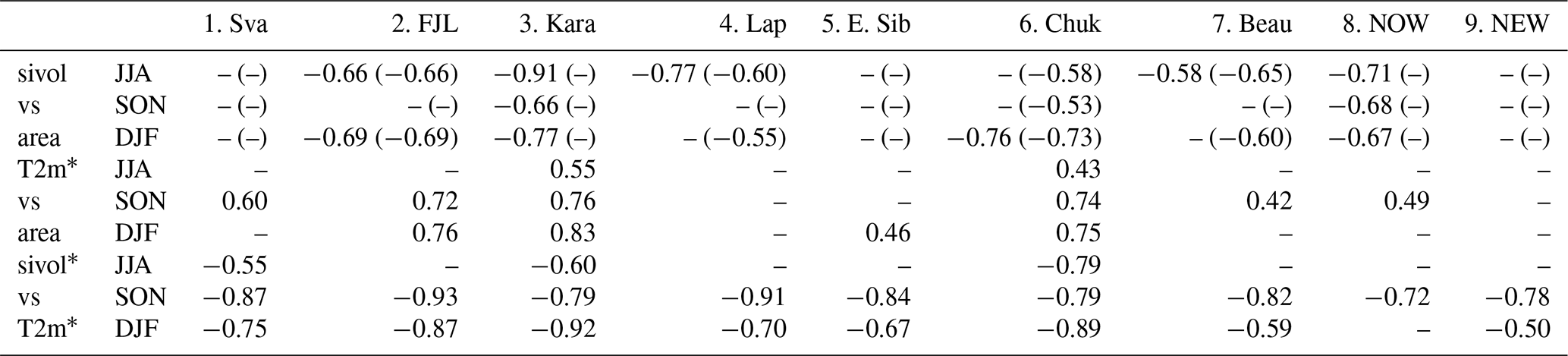
In observations, Sumata et al. (2023) identified a regime shift in sea ice when the sea ice draft passes below the 1.3 m threshold, which corresponds to sea ice becoming thinner than approximately 1.5 m. This 1.5 m thickness threshold has also been seen in models: Athanase et al. (2025) argued that it is because it matches the sea ice concentration threshold at which the free drift parameterisation is switched on or off (approximately 80 %), while in some sea ice models at 1.5 m thickness the sea ice albedo parameterisation changes (Rousset et al., 2015). Looking only at the regions with a significant across-model correlation between thickness and polynya activity, we do see a suggestion of larger polynya activity for models with mean thickness below 1.5 m (Appendix Fig. A4, 1.5 m is the black horizontal line). This is however not a clean cut: in all regions, some models exhibit polynya activity even at thicknesses larger than 2 m while others still have no polynya below 1 m thickness. The thickness bias alone cannot explain the polynya activity bias.

To summarise, (1) there is no consistent across-model relationship between polynya area and sea ice thickness biases, not even in winter; and (2) there seems to be some clustering of the biases by sea ice model (Fig. 4). A clue that the polynya bias is not linked to one specific, physical process, but rather caused by a deep model-dependent bias, e.g. in its treatment of thermodynamics, would be an across-model link between polynya bias and the model's equilibrium climate sensitivity (ECS). We do find a significant correlation of 0.76 between the ECS of Zelinka et al. (2020) and the pan-Arctic polynya area, with the caveat that there are only 9 models in common in our studies. That is, this link may not be robust, but it is encouraging. Let us therefore investigate more closely the impact of the sea ice component of the models. Two sea ice models are over-represented in our study: the Los Alamos sea ice model CICE (Hunke et al., 2017) and the Louvain-La-Neuve sea ice model LIM (Rousset et al., 2015), with the latter typically simulating larger polynya areas (see Sect. 3). Many parameters can be relevant for polynyas, sometimes with opposite results: Chevallier et al. (2017) found for example that, in ocean reanalyses, having several thickness categories (as CICE does) resulted in a thinner ice, but so did having a low “P^∗” ice strength (as LIM does). One crucial point is that the two models have completely different thermodynamics treatments and surface processes included, with CICE having long included a scheme for melt ponds. As a result, CICE has a rather realistic sea ice growth/melt (Sun and Solomon, 2024) when compared to observations, whereas in LIM both growth and melt are faster and with a larger amplitude than expected (Uotila et al., 2017). This would explain LIM's large and frequent polynyas.

The dynamics treatments also differ between LIM and CICE. Winter Arctic polynyas typically form in response to strong winds (Smith and Barber, 2007), making an accurate representation of wind forcing on sea ice crucial for simulating polynya openings. In sea ice models, it is the rheological formulation and roughness (or drag) that control how efficiently wind forcing is transmitted into sea ice motion. Ocean reanalyses with a low air–ice drag coefficient (such as LIM) have a slower sea ice drift (Chevallier et al., 2017), i.e. should be harder to open by wind divergence. There is also an ice–ocean drag coefficient; ocean reanalyses with a low ice–ocean drag coefficient (such as CICE) have a thinner sea ice (Chevallier et al., 2017), i.e. should be easier to open by wind divergence. Besides, the sea ice models use different rheologies: elastic-viscous-plastic for CICE and LIM3 but viscous-plastic for LIM2. This could impact sea ice deformation on short time scales and its sensitivity to wind stress. All these hypotheses however assume that models, as in reality, form Arctic polynyas in response to winds rather than thermodynamics forcing; we verify this assumption in the next subsection.

4.2 Winds and air temperature

There is no across-model correlation, even when excluding the polynya area outlier AWI-CM-1-MR, between the 45-year mean wind characteristics and the polynya area in any region. However, most models have strong significant correlations between the time series of the polynya area and that of the wind speed and/or the wind components (Appendix Tables A6 to A8). Correlations with the wind speed, both its mean and extreme, are widespread in the Eurasian Arctic, from Svalbard to the East Siberian sea, whereby stronger wind speeds are associated with larger polynya areas. This is in agreement with e.g. Smith and Barber (2007); Wong et al. (2026).

In the other regions, fewer models have correlations between the winter wind and polynya time series. In the Chukchi and Beaufort seas and in the North East Water polynya, the models that have such correlation tend to have a negative correlation with mean U and the 10th percentile of U, and positive with mean V and the 90th percentile of V 90th or negative with the 10th percentile of V (Appendix Tables A7 and A8), i.e. the stronger the northwestward winds, the larger the polynya area. The correlation with the northward winds is in agreement with real-world polynya observations; Lee et al. (2023) in particular showed that the few observed winter polynya events in NEW were entirely driven by northward (southerly) winds mechanically redistributing the thick ice. The correlation with the westward winds both for NEW and the Pacific side seems counterintuitive, but in observations Peralta-Ferriz and Woodgate (2017) found that enhanced westward winds lead to a stronger inflow of Pacific Water through Bering Strait, i.e. a larger supply of upper-ocean heat that can melt the sea ice in the Chukchi and Beaufort regions. Lavoie et al. (2022) found that some CMIP6 models do not represent any Pacific Water; this may explain why the correlation is not more widespread among our models. Similarly, westward winds would impact the models' (re)circulation of Atlantic Water north of Fram Strait, which may explain the occasional model's correlation with the NEW polynya area. Finally, as in the real world, the North Water Polynya is associated with southward winds, albeit only seen for the high horizontal resolution models (Appendix Table A8). The other models most likely are too coarse to properly represent the Nares Strait geography or because the resolution of the atmosphere component directly impacts the representation of the most extreme winds (Huot et al., 2021), crucial for Greenland polynyas (Smith and Barber, 2007). Moore (2021) explicitly states that a resolution of at least 9 km in the atmosphere is required; for comparison, the high resolution version of the CMIP6 models that participated in HighResMIP is of the order of 25 km (Haarsma et al., 2016).

In contrast, we find strong across-model correlations between air temperature and polynya area in all regions except the Laptev Sea and North East Water polynya (Table 3). Correlations with the same winter are to be expected, since e.g. Wong et al. (2026) found a similar relationships in observations in the Arctic, which they explained as warm air thinning the ice, preconditioning the region for polynya opening. This is consistent with the strong across-model negative correlation between air temperature and sea ice thickness in winter, and that between thickness and polynya area discussed in the previous section (Table 3). We however find hardly any across-model relationship in summer, even though summer thickness and polynya area were strongly associated, which further suggests that a generally thin summer ice is not a driver but a consequence of large polynya activity in a model.

We rather find large across-model relationships between autumn air temperature and both winter polynya area and autumn sea ice thickness throughout the Arctic (Table 3, middle), with mean autumn air temperature being the only one correlated with mean polynya area in Svalbard (R = 0.60), the Beaufort Sea (R = 0.42) and the North Water Polynya (R = 0.49). In all regions, the absolute value of the correlation between autumn air temperature and autumn sea ice thickness exceeds 0.7. Interestingly, this is similar to what Zhou et al. (2022) found in observations for open water polynyas in the Southern Ocean: the subsequent opening of the polynya was detectable already in the autumn as a thin ice anomaly, which pre-conditioned the region for opening with the winds acting as final trigger.

To summarise, as in observations, we find significant relationships in each model between polynya area and wind speed or direction. The most important wind component depends on the location, but also on the horizontal resolution of the model in narrow locations such as the Canadian archipelago. We also find a large contribution of the model's overall temperature bias via its impact on sea ice thickness, with warmer models having thinner ice in autumn. Determining whether individual models are actively melting sea ice in autumn or simply delaying its growth is beyond the scope of this study. The outcome is the same: a sea ice in which it is easier to open polynyas in the subsequent winter. Across-model correlations between polynya area and sea ice thickness year-round, along with the autocorrelation of sea ice, perpetuate the polynya cycle, resulting in some models being more polynya-prone than others. We finish this manuscript with an analysis of the potential impacts of this diffence in overall polynya behaviour on the ocean.

5 Do winter Arctic polynyas impact the modelled ocean?

One of the motivations for this study was the finding of Heuzé et al. (2023) that most CMIP6 models have no dense overflow representation, and that the few models that do have overflows have them only in Saint Anna Trough, in the Kara Sea, even though they seemed to also have polynyas in the Laptev Sea. They further found that few models have dense water at the bottom of the shelf break, below the expected polynya area, and that the properties of this dense water were inconsistently biased. They therefore suspected that something had gone wrong in the ocean–sea ice coupling, suggesting a disconnect between the representation of polynyas in models and the simulated ocean properties. We finish this study by briefly expanding on their analysis.

5.1 Polynya activity does not seem to impact the mean hydrographic biases

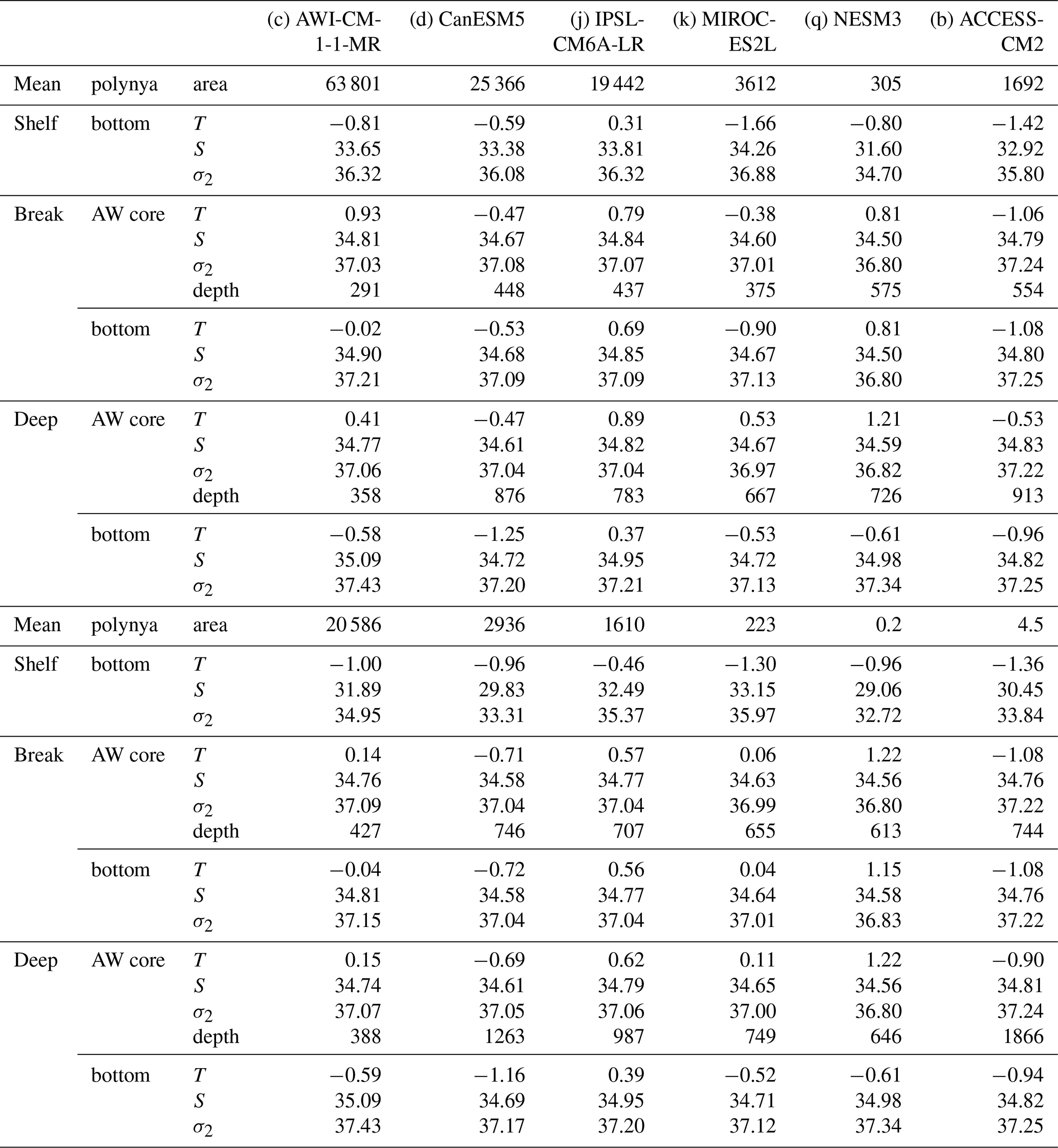
We contrast the three models with most polynya activity (red on Figs. 7 and 8) to the three with least activity (blue). We limit our analysis to the Kara and Laptev seas, two regions that are regularly cited in observational and modelling studies as being highly productive in terms of sea ice formation and brine rejection, which impact dense water formation and deep ocean ventilation (e.g. Tamura and Ohshima, 2011; Itkin et al., 2015; Preußer et al., 2016). In the Kara Sea, the mean temperature at the surface of the shelf break is colder in the models with least activity: all three are below −1 °C (blue on Fig. 7), whereas the surface of the most active models is between −0.8 to +1.2 °C. That they are not at freezing temperature, whether because of warm water upwelling or warm air, suggests that brine rejection will be hindered. This surface temperature difference is also consistent with our earlier finding of thinner ice and stronger seasonal cycle being associated with higher polynya activity, although whether the upper ocean is systematically warmer because sea ice melts in summer, or sea ice melts in summer because the ocean is warmer, we cannot tell from these data. It may also be a coincidence in this subsample of models, since the other depth levels, properties and regions show no consistent behaviour. In fact, considering the temperature on the shelf, the lines of the least (blue) and most active (red) models cross already at 40 m depth. And since even at the surface, the salinity biases are inconsistent between these models on the continental shelf, so is their density (Fig. 7, left). In particular, the models with most polynya activity do not have denser water at the bottom of the shelf than the models with least activity: of the six models, the densest is MIROC-ES2L, among the least active models (36.88 kg m⁻³, Appendix Table A9). Therefore, it comes as no surprise that there is no consistency at the shelf break, in any of the properties, nor in the deep basin. Although it seems at first glance that the Atlantic Water core is deeper off-shelf in the least active models (blue in Fig. 7, right), we find that the core depth varies from 358 to 876 m in the most active models, and 667 to 917 m in the least active, i.e. their ranges overlap (Appendix Table A9).

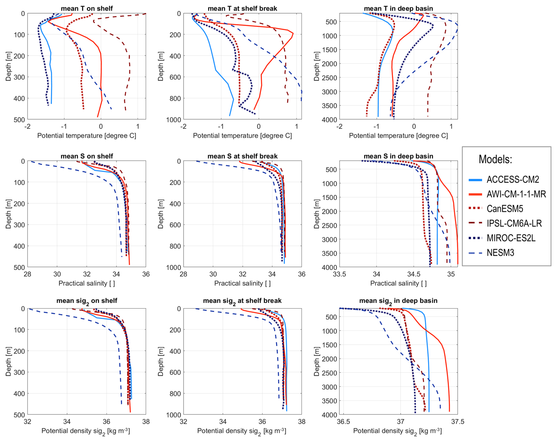
Figure 7 In the Kara Sea, for the three models with most (red) and least (blue) polynya activity, profiles of potential temperature (T, top), practical salinity (S, middle) and potential density anomaly σ₂ (sig₂, bottom) on the continental shelf (left), at the shelf break (centre), and in the deep basin (right). For the values and identifying which model is which, see Appendix Table A9. Note that in the deep basin, the depth axis starts at 200 m depth.

Figure 8 Same as Fig. 7 but for the Laptev Sea.

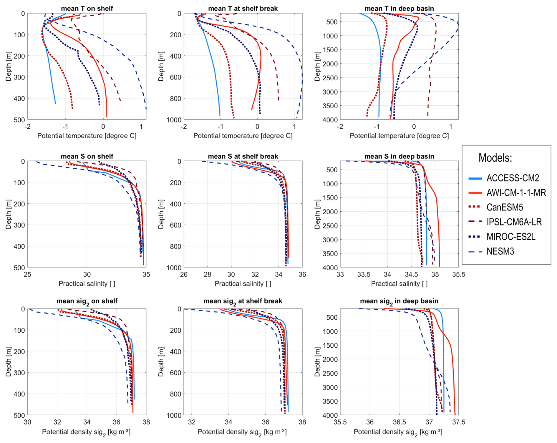
CMIP6 models have 10 times smaller polynya areas in the Laptev Sea than in the Kara Sea, and they are more sporadic (see Sect. 3). These differences appear to have no impact on the ocean profiles (Fig. 8). We find again that the only consistent clustering is in the temperature at the very surface of the continental shelf, with the least active models being colder than the most active ones (blue, below −1 °C; red, −0.8 to 0 °C). It is worth noting again that in the most active models, these temperatures are above freezing, i.e. not compatible with sea ice production and brine rejection. The bias order is not maintained with depth and there is no consistent bias in salinity, so the density at the bottom of the shelf does not significantly differ between the three most polynya-active and three least active models; again, the densest model is in fact MIROC-ES2L, among the least active models (35.97 kg m⁻³, Appendix Table A9). We find no consistency in the Atlantic Water core or bottom properties, either at the shelf break or in the deep basin (Fig. 8).

5.2 Polynya activity can have a short-lived impact on ocean properties in individual models

In particular in the Laptev Sea, where polynyas are simulated less frequently, it may be that taking the 45-year average masks the effect of polynyas on the water column. We therefore correlate the time series of polynya area and ocean properties, considering both the yearly-mean properties and the different seasons to account for the time the dense water may need to travel from the shelf to the deep basin. In observations, this takes 3 to 6 months (Ivanov and Golovin, 2007; Luneva et al., 2020). In the two active models CanESM5 and IPSL-CM6A-LR, this takes up to one year, with maximum correlations found between polynya activity and properties at the bottom of the deep ocean in both Kara and Laptev in the subsequent autumn (Table 4). In AWI-CM-1-1-MR, correlations are rather with the yearly value or that of the same winter; it is not impossible that in that very high resolution model, jets of dense water reach the deep basin shortly after their formation. The active models tend to agree on the sign of the correlations, with more polynya activity being associated with warmer and fresher deep basins. AWI-CM-1-1-MR and CanESM5 also agree that more polynya activity is associated with warmer and less-dense waters at the bottom of the shelf and at the bottom of the shelf break, in both seas. This is unexpected since polynya activity is supposed to generate dense water (Morales Maqueda et al., 2004). Even when polynyas have been observed to result in warmer deep waters, it was in conjunction with high salinities (Vivier et al., 2024). Models do not systematically have a correlation between polynya activity and the bottom salinity there, but when they do, this correlation is negative, i.e. more polynya activity is surprisingly associated with fresher waters (Table 4, bottom S). This would be consistent with polynyas opening by melting the ice, i.e. sensible heat polynyas, rather opening dynamically in response to strong winds, i.e. latent heat polynyas (Morales Maqueda et al., 2004). Note that the third of the most active polynya models, IPSL-CM6A-LR, has no such correlation between polynya activity and bottom properties (Table 4), even though it uses the same ocean and sea ice model as CanESM5, albeit a newer version of it. In the “real” Arctic, there are no purely sensible heat polynyas, but there are hybrid ones that switch modes while open from latent heat to sensible heat; after the switch, dense water production has been observed to stop (Hirano et al., 2016). Models simulating sensible heat polynyas would be consistent with the lack of connection between polynya activity and bottom properties.

Table 4 For the models with most (left) and least (right) polynya activity, in the Kara (top) and Laptev (bottom) seas, maximum correlation between the 1979–2024 winter polynya area time series and that of the ocean properties on the continental shelf, at the shelf break, and in the deep basin, in the Atlantic Water core and at the bottom cell. “–” indicates that no significant correlation (at 95 %) could be found. We show only the maximum correlation, in absolute value, and indicate whether this correlation corresponds to the yearly mean ocean property (Year), to that of the same winter as the polynya (DJF), or to the subsequent spring (MAM), summer (JJA) or autumn (SON).

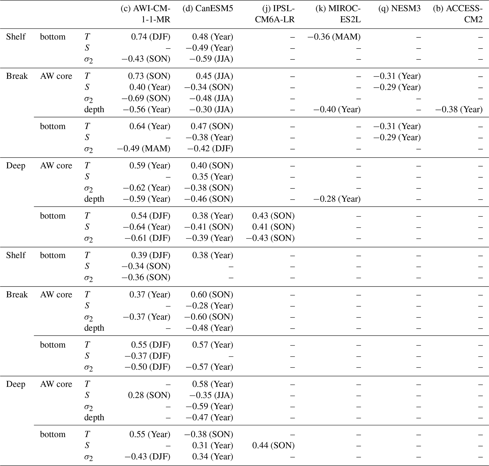
Finally, both most and least active models have negative correlations at the Kara Sea shelf break between the Atlantic Water core depth and polynya activity, i.e. the more polynya activity the shallower the core (Table 4, AW core depth). In the real Eurasian Arctic, the dense water cascade entrains Atlantic Water as it flows off the shelf there, which results in a cooling and deepening of the Atlantic Water core (e.g. Woodgate et al., 2001; Dmitrenko et al., 2014). Heuzé et al. (2023) found that CMIP6 models systematically had too deep an Atlantic Water core, often sitting below the shelf break depth, and that this bias was the result of a biased Atlantic Water inflow through Fram Strait that was not corrected by ventilation in the Arctic, since there was virtually no ventilation. It may therefore be that polynya activity momentarily corrects that advected Atlantic Water bias. However, the lack of consistency between polynya activity and both temperature and salinity, most likely a result of how models open their polynya, suggests that polynyas cannot correct the other ocean biases.

6 Summary and final comments

Although winter Arctic polynyas play a crucial role for all components of the Arctic climate and its ecosystem (Smith and Barber, 2007), and that satellite observations have revealed a strong increase in their area since 1970s (Wong et al., 2026), to the best of our knowledge, this study was first to evaluate the representation of winter Arctic polynyas in any CMIP generation. We detected polynyas using their daily sea ice concentration since daily sea ice thickness is not widely available in CMIP6, and found that the majority of models overestimate the polynya area while they underestimate their frequencies. The exception was the very high resolution model AWI-CM-1-1-MR (∼ 100 km² grid cells,  Semmler et al., 2020) which was overestimating both, in all regions. The spatial distribution matches that of observational studies relying on sea ice concentration, but obviously misses some thin-ice polynyas that are better detected via sea ice thickness or surface fluxes (e.g. Tamura and Ohshima, 2011; Preußer et al., 2016). Unfortunately in CMIP6, only daily sea ice concentration was both widely available and reliable. The temporal resolution obviously mattered as well, with polynya areas computed from monthly sea ice concentration being lower than those from the daily, yet usually correlated with each other. That is, it would technically be possible to infer daily results from monthly output in order to increase the amount of models available; we however advise against this, as the relationship was region-dependent, and are rather looking forward to the planned more widespread release of daily output in CMIP7 (Fox-Kemper et al., 2025).

Despite the apparent link with both temporal and spatial resolution, we find that models tend to cluster by sea ice model. This is not that surprising, since polynya dynamics are strongly influenced by the sea ice physics and their rheologies. Besides, although most winter Arctic polynyas are supposed to be wind-driven (Morales Maqueda et al., 2004), we found no across-model relationship between wind bias and polynya bias. The two most common sea ice models, CICE and LIM, have different drag coefficients and thermodynamics schemes that make it harder to open polynyas in response to winds but easier with thermodynamics, respectively (Hunke et al., 2017; Uotila et al., 2017; Chevallier et al., 2017). We find that the LIM models are among those with the largest polynyas, but also the largest sea ice seasonal cycle. In fact, across models, we find that the larger polynya areas are associated with warmer autumns, leading to thinner ice/delayed ice growth in the large seasonally ice free regions, which are thus preconditioned for opening polynya in the winter. Thermodynamics do matter in observations, even for wind-driven polynyas, as a warmer atmosphere preconditions the region for polynya opening (Wong et al., 2026), especially in the autumn (Zhou et al., 2022). Our results however show a lack of across-model relationship between wind and polynya activity, i.e. thermodynamics does not only matter for preconditioning but is also the trigger. As CMIP6 models project an increase in wind speed in the Arctic and in the transfer of wind stress to the ice, notably in winter (Muilwijk et al., 2024), one would expect a continued increase in “real” polynya area in the future. Given the models' lack of agreement on recent polynya trends (Fig. 4) and suspected incorrect opening mechanism, we prefer leaving future projections out of this study.

Finally, rather disappointingly, we find that polynya activity does not seem to affect the representation of the water column in CMIP6 models, in agreement with the preliminary findings of Heuzé et al. (2023). Even by limiting the water column analysis to the three most and three least polynya-active models, we found no consistent relationship between polynya activity and properties on the continental shelf, at the shelf break, or in the deep basin. In particular, even though real-world polynyas are hotspots of sea ice production (Tamura and Ohshima, 2011) and therefore result in dense water at the bottom of the shelf (Vivier et al., 2024), our densest model was one of the least polynya-active. At the individual model level, we even found negative correlations between polynya activity and bottom density, i.e. the larger the polynya, the less-dense the shelf water of that year, further suggesting that polynyas in CMIP6 models are the result of sea ice melt rather than wind-driven dynamics opening. That is, CMIP6 models seem to be opening sensible heat polynyas in the Arctic, where all observed polynyas are primarily wind-driven latent-heat or hybrid (Wong et al., 2026). Another surprising result was widespread negative correlations between polynya activity in the Eurasian Arctic and Atlantic Water core depth, i.e. the larger the polynya, the shallower the core, i.e. the opposite of the real-world (e.g. Dmitrenko et al., 2014). Our optimistic interpretation is that polynyas momentarily reduce the deep bias detected by Heuzé et al. (2023), but due to polynya's intermittent nature and their apparent wrong formation process, polynyas cannot fix the overall model bias, caused by advected errors through Fram Strait.

How to fix these biases? A higher resolution is the obvious answer, both in the ocean to represent the complex coastline geometry and in the atmosphere for the strong winds (Huot et al., 2021; Moore, 2021), but it is unrealistic. In fact, some modelling centres have even decided to not increase their model resolution beyond ∼ 1°, as the marginal improvement in the global climate representation cannot justify the increased climate footprint of the simulation (OMIP protocol for CMIP7, to be submitted soon). Besides, the highest resolution model in our study was a clear outlier. One option that seems promising is the better representation of land-fast ice (Itkin et al., 2015), which is crucial for polynya development in the real Arctic (Morales Maqueda et al., 2004) but usually not captured in models. It is also possible that the biases will fix themselves: as polynya area increases (Wong et al., 2026) and the shelf break keeps warming (Ingvaldsen et al., 2021), real-world winter Arctic polynyas may soon become open-ocean polynyas that open through thermodynamics, which models already do, making CMIP polynya representation and projection more trustworthy.

Appendix A

Dix et al. (2019)Semmler et al. (2018)Swart et al. (2019b)EC-Earth Consortium (EC-Earth) (2020a)EC-Earth Consortium (EC-Earth) (2020b)EC-Earth Consortium (EC-Earth) (2020c)EC-Earth Consortium (EC-Earth) (2019b)Boucher et al. (2020a)Boucher et al. (2018)Hajima et al. (2019)Tatebe and Watanabe (2018)Neubauer et al. (2019)Jungclaus et al. (2019)Wieners et al. (2019)Yukimoto et al. (2019b)Cao and Wang (2019)Seland et al. (2019)Bentsen et al. (2019)

Table A1 For the models with daily sea ice concentration output: Model name, Ensemble members used in this study and their corresponding Shared Socio-economic Pathway (SSP) run, and the Dataset DOI of the CMIP6 runs along with its reference. n/a: not applicable.

Dix et al. (2019)Ziehn et al. (2019)Rong (2019)Chai (2020)Danabasoglu (2019a)Danabasoglu (2019b)Huang (2019)Lovato and Peano (2020)Lovato et al. (2021)Voldoire (2019)Voldoire (2018)Seferian (2018)Swart et al. (2019c)Swart et al. (2019b)EC-Earth Consortium (EC-Earth) (2020a)EC-Earth Consortium (EC-Earth) (2020b)EC-Earth Consortium (EC-Earth) (2020c)EC-Earth Consortium (EC-Earth) (2019b)EC-Earth Consortium (EC-Earth) (2019a)Song et al. (2019)Ridley et al. (2018)Ridley et al. (2019)Boucher et al. (2018)Hajima et al. (2019)Tatebe and Watanabe (2018)Neubauer et al. (2019)Jungclaus et al. (2019)Wieners et al. (2019)Yukimoto et al. (2019b)Cao and Wang (2019)Bethke et al. (2019)Seland et al. (2019)Bentsen et al. (2019)Lee and Liang (2019)Tang et al. (2019)

Table A2 Same as Table A1 but for the models with monthly sea ice concentration output. n/a: not applicable.

Table A3 Coordinates of the nine regions used in this study, as per Wong et al. (2026). Also shown on Fig. 3a.

Figure A1 Same as Fig. 2 but for the nine regions analysed in this paper: 1. Svalbard, 2. Franz Josef Land, 3. the Kara Sea, 4. the Laptev Sea, 5. the East Siberian Sea, 6. the Chukchi Sea, 7. the Beaufort Sea, 8. the North Water Polynya and 9. the North East Water Polynya. Regions shown on Fig. 3a and defined in Appendix Table A3.

Figure A2 Same as Fig. 4 but including AWI-CM-1-1-MR.

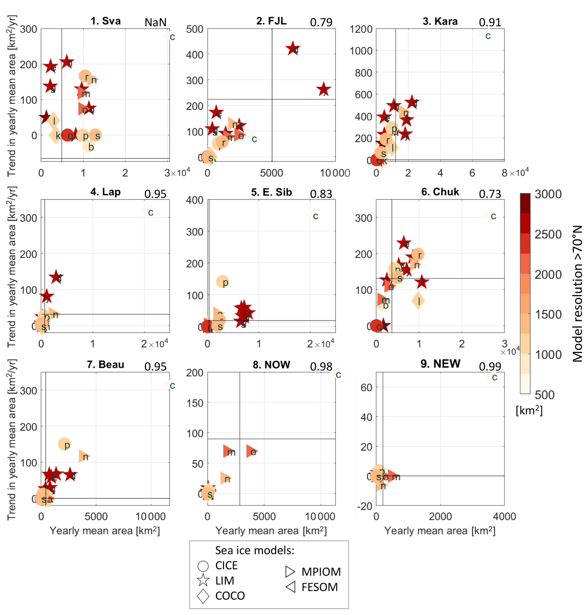
Table A4 Values shown on Fig. 4. Top rows: 1979–2024 mean of the yearly winter (December–March) mean polynya area, in km². Bottom rows: 1979–2024 trends in yearly winter mean polynya area, in km² yr⁻¹, at 95 % significance; “NaN” if insignificant.

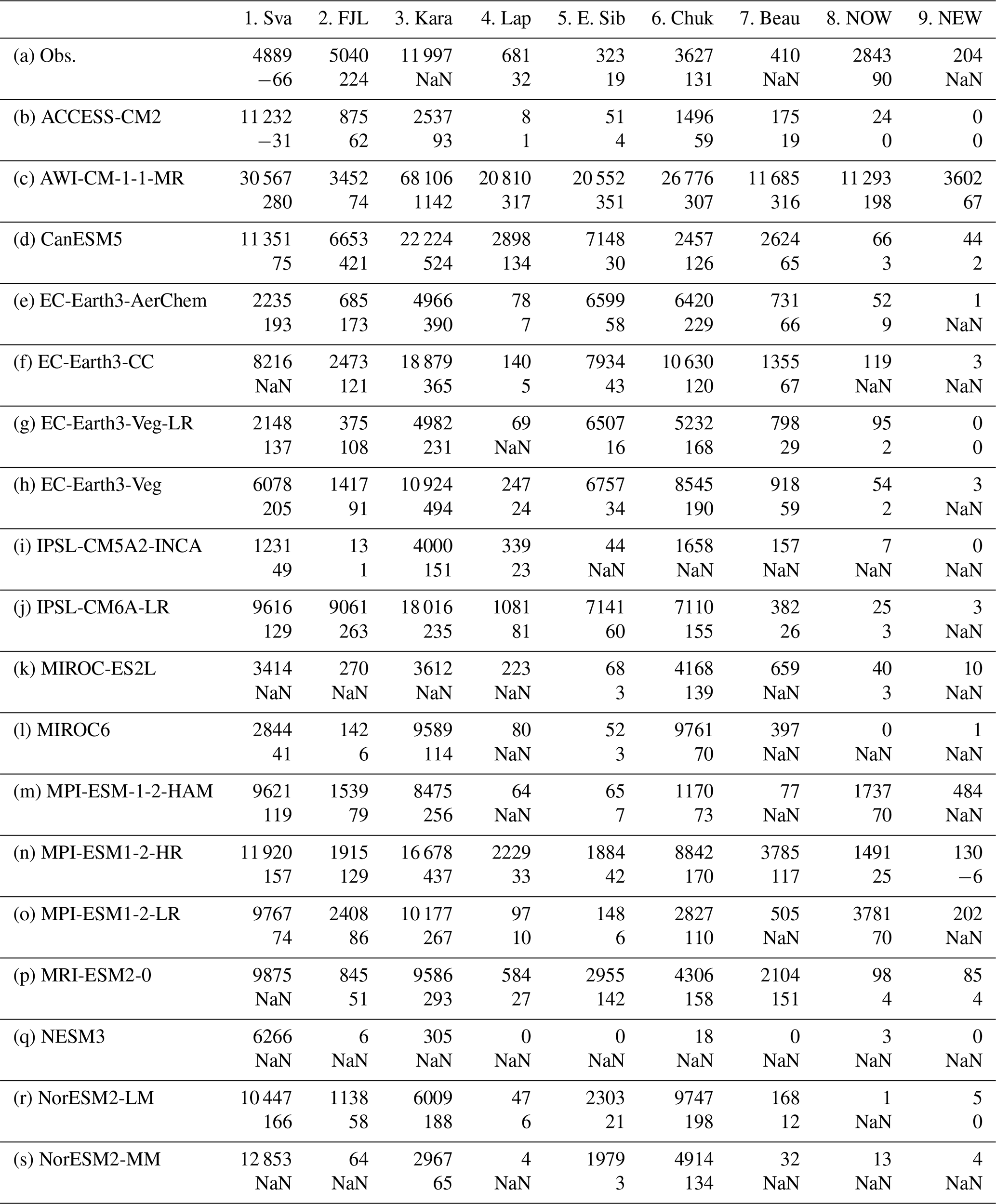
Table A5 For each model, in each region, correlation (95 % significant) between the time series of the winter (DJFM) mean polynya area and that of the previous summer (JJA), previous autumn (SON), and same winter (DJFM) mean sea ice thickness. “–” indicates non significant correlations.

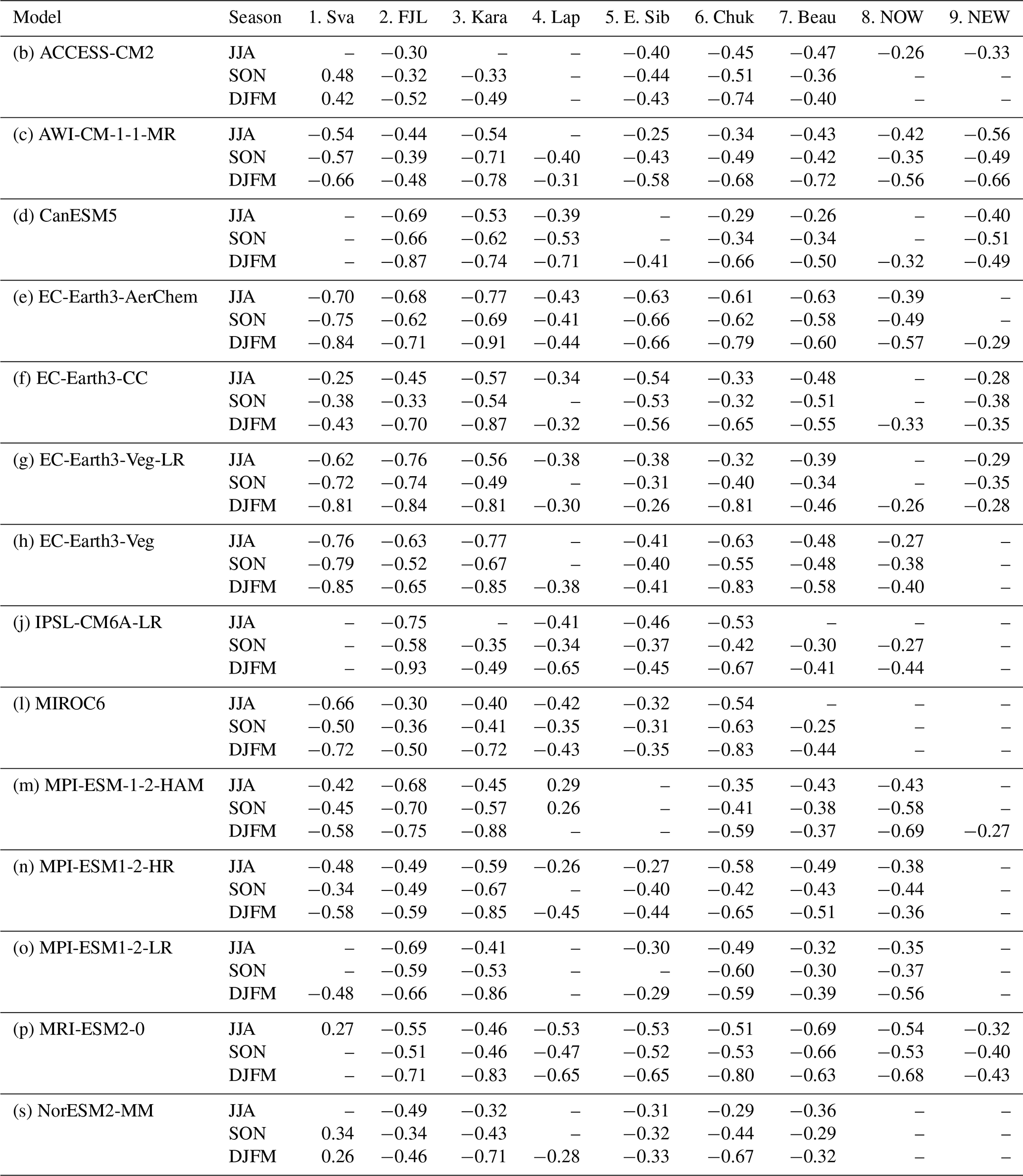
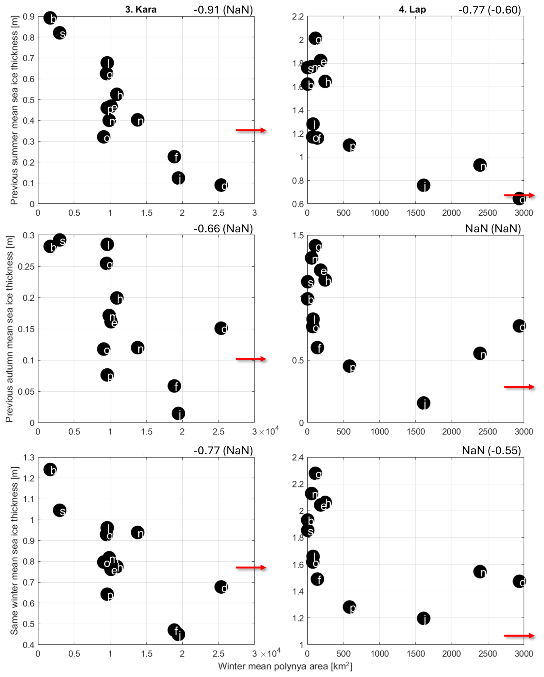
Figure A3 In the Kara (left) and Laptev (right) sea regions, across-model relationship between the 1979–2024 mean of the winter mean polynya area (x-axis) and the 1979–2024 mean sea ice thickness (y-axis) in summer (top), autumn (centre), and winter (bottom). Models referred to with same letters as on Fig. 3. Numbers in the top right corner of each panel is the correlation between the two (95 % significance), with that in brackets when the outlier AWI-CM-1-1-MR is included, as per Table 3. Red arrow indicates AWI-CM-1-1-MR sea ice thickness value and point in the direction of its polynya area; see area value on previous figures or in e.g. Appendix Table A4.

Figure A4 For all regions (colours), across-model relationship between the 1979–2024 mean of the winter mean polynya area (x-axis) and the 1979–2024 mean sea ice thickness (y-axis) in summer (top), and winter (bottom), shown only if there is a significant relationship between the two in the region. See also Table 3. Models referred to with same letters as on Fig. 3. Black horizontal line is the 1.5 m sea thickness threshold discussed in the main text.

Table A6 For each model, in each region, correlation (95 % significant) between the time series of the winter (DJFM) mean polynya area and that of the same winter mean and 90th percentile wind speed. “–” indicates non significant correlations.

Table A7 For each model, in each region, correlation (95 % significant) between the time series of the winter (DJFM) mean polynya area and that of the same winter mean, 10th and 90th percentiles zonal wind (i.e extreme west- and eastward, respectively). “–” indicates non significant correlations.

Table A8 Same as Table A7 but for the meridional wind; 10th and 90th percentile are extreme south- and northward, respectively.

Table A9 For the models with most (left) and least (right) polynya activity, in the Kara (top) and Laptev (bottom) seas, 45-year mean polynya area in km² and 45-year mean properties on the continental shelf, at the shelf break, and in the deep basin, in the Atlantic Water core and at the bottom cell. Potential temperature T is in ° C; practical salinity S has no unit; potential density anomaly σ₂ is in kg m⁻³; depth is in m.