The importance of initial conditions in seasonal predictions of Antarctic sea ice

Accurate Antarctic sea-ice forecasts are crucial for climate monitoring and operational planning, yet they remain challenging due to model biases and complex ice-ocean-atmosphere interactions. The two versions of the Australian Bureau of Meteorology's seasonal forecast system, ACCESS-S1 and ACCESS-S2, use identical model configuration but differ only in their initial conditions; primarily in that ACCESS-S2 does not assimilate sea-ice observations, whereas ACCESS-S1 does. This provides a convenient opportunistic experiment to assess the role of initial conditions on Antarctic sea-ice forecasts using more than 20 years of fully coupled simulations with two nine-member ensembles. Our analysis reveals that both systems experience an extended melt season and delayed growth phase compared with observations. This leads to a significant negative sea-ice extent bias, which is reduced in ACCESS-S1 by the data assimilation system. The impact of the differing initial conditions on forecast errors varies dramatically by season: summer and autumn (January–April) sea-ice initial conditions provide predictive skill for up to three months, with February initial conditions being particularly crucial. In contrast, winter forecasts of the two systems are statistically indistinguishable after only two weeks. Regional analysis of forecast skill suggests that this winter predictive skill barrier is most dramatic over East Antarctica, where even ACCESS-S1 shows negative skill. These findings highlight the critical importance of comprehensive year-round sampling in predictability studies and suggest that operational sea-ice data assimilation efforts should prioritise the summer-autumn period when initial conditions have maximum impact on forecast skill.

1 Introduction

Accurately modelling Antarctic sea ice is essential for understanding climate processes and improving climate projections to inform adaptation strategies. Accurate sub-seasonal to seasonal forecasts are also crucial for operational contingency planning in and around the Antarctic continent, including scientific missions, fisheries, and tourism (De Silva et al., 2020; Wagner et al., 2020). Improvements in modelled sea ice might also help improve weather forecasts over and away from sea-ice regions (Rinke et al., 2006; Wang et al., 2024; Semmler et al., 2016).

However, progress in Antarctic sea-ice forecasting has lagged behind Arctic sea-ice forecasting due to model biases and inherent large variability and complexity (Zampieri et al., 2019; Gao et al., 2024). Dynamical seasonal forecasts of summer Antarctic sea ice have been shown to perform worse than relatively simple statistical methods (Massonnet et al., 2023) and machine learning approaches (e.g. Dong et al., 2024; Lin et al., 2025), which also underscores the need for better understanding and physical modelling of sea-ice dynamics and drivers of its variability.

Good initial conditions are an essential element for a good forecast; however, it is not entirely known to what extent accurate sea-ice initial conditions affect the quality of the forecast and at what timescales. Exploring seasonal predictions of Arctic sea ice, Guemas et al. (2016) found that sea-ice initial conditions are important in autumn to predict summer Arctic sea ice, but the impact was not as dramatic when predicting winter Arctic sea ice. Day et al. (2014) also found seasonally-varying differences in the effect of initialisation, noting that accurate Arctic sea-ice thickness leads to improved sea-ice forecasts initialised in July but not when initialised in January.

For the Antarctic, Holland et al. (2013) studied the initial-value predictability of Antarctic sea ice in a perfect model study using the Community Climate System Model Version 3 model. They found that sea-ice and ocean initial conditions provide predictive information to forecast sea-ice edge location several months in advance and that some predictability is retained for up to two years thanks to ocean heat content anomalies that are advected eastward. Similarly, Morioka et al. (2022) studied decadal forecasts of Antarctic sea ice and found that initialising ocean and sea ice improved the correlation between simulated and observed sea-ice concentration evolution in the Amundsen–Bellingshausen Sea. This is in contrast with Marchi et al. (2020), who ran perfect model experiments to argue that uncertainty in the predicted atmospheric state and evolution is the main driver of uncertainty in Antarctic sea-ice extent prediction on seasonal timescales, with sea-ice and ocean initial conditions having lesser importance. More recently, Xiu et al. (2025) contrasted Antarctic sea ice hindcasts based on different data assimilation sources. They concluded that hindcasts initialised only with atmospheric data led to good predictions of sea-ice area in many regions that were comparable, if not better, than hindcasts initialised only with ocean data or with ocean and sea-ice concentration data. Furthermore, they found that assimilation of sea-ice concentration data offered little benefit on top of assimilation of ocean data.

It is hard to compare these studies since they are based on forecasts initialised at different times of the year and different frameworks. Holland et al. (2013) ran 20 ensemble members initialised on the 1 January of a particular year, Marchi et al. (2020) ran forecasts from the 1 March and 1 September, and Morioka et al. (2022) ran forecasts only from the 1 March. Xiu et al. (2025) was the most comprehensive study, using hindcasts initialised on the 1 January, April, July and October. Marchi et al. (2020) also used a coupled ocean–sea-ice model instead of a fully coupled model like Holland et al. (2013) and Xiu et al. (2025) did. Morioka et al. (2022) and Xiu et al. (2025) both compared forecast with observations, but the former initialised the model using observed sea-ice initial conditions while the latter used initial conditions derived from a data assimilation system. On the other hand, Marchi et al. (2020) and Holland et al. (2013) were perfect model studies.

In October 2021 the Australian Bureau of Meteorology (BoM) upgraded the Australian Community Climate and Earth System Simulator – Seasonal (ACCESS-S) from version S1 to S2 (Wedd et al., 2022). While the base model remained the same, the change in version was focused on using ocean, sea-ice and land initial conditions generated by the BoM instead of depending on the UK Met Office. Crucially, compared to ACCESS-S1, ACCESS-S2 does not assimilate sea-ice observations, so sea ice is only affected by the ocean and atmospheric data assimilation via the coupled integration.

Since model configuration is identical between ACCESS-S1 and ACCESS-S2, they form an “opportunistic experiment” where the same forecasting model was run over a long period of time with multiple ensemble forecasts initialised throughout the year, with the only difference being the initial conditions. This provides an opportunity to test the effect of sea-ice initial conditions on the forecast of sea-ice concentrations and the climate.

In this study we compare sea-ice hindcasts produced by ACCESS-S1 and ACCESS-S2. We focus on seasonality of errors and biases and the effect of the data assimilation system. This comparison will inform future work with the prediction system as a research tool to better understand the dynamics and variability of the Antarctic sea ice and its impacts on the climate system as well as to explore the potential of using its sea-ice forecasts for decision-making. The work will also serve as a benchmark for future prediction systems to attempt to improve upon.

2 Data and methods

2.1 Forecasting systems

ACCESS-S2 (Wedd et al., 2022) is the BoM's seasonal forecast system which became operational in October 2021, replacing the ACCESS-S1 system (Hudson et al., 2017). The model components of both ACCESS-S2 and ACCESS-S1 are identical with the same numbers of levels and resolution. They consist of the Global Atmosphere 6.0 (GA6) (Williams et al., 2015; Waters et al., 2017), the Unified Model's Global Land 6.0 (Best et al., 2011; Waters et al., 2017), NEMO Global Ocean 5.0 (Gurvan et al., 2013; Megann et al., 2014) and Global Sea Ice 6.0 (CICE; Rae et al., 2015). The atmosphere has a N216 horizontal resolution (∼60 km in the mid-latitudes) with 85 vertical levels. The land model uses the same horizontal grid as the atmosphere with four soil levels. The ocean component has a nominal horizontal resolution of $\mathrm{1}/\mathrm{4}$° with 75 vertical levels. The sea-ice component, based on CICE version 4.1, has the same resolution as the ocean component and five sea-ice thickness categories as well as an open water category.

Both systems take atmospheric initial conditions derived from ERA-interim (Dee et al., 2011) for their hindcasts. The only difference between the hindcasts of the two systems are the ocean and sea-ice initial conditions and the ensemble generation procedure.

ACCESS-S1's ocean and sea-ice initial conditions come from the Met Office FOAM system, which uses a multivariate, incremental three-dimensional variational (3D-Var), first-guess-at-appropriate-time (FGAT) data assimilation scheme (Waters et al., 2015) and assimilates sea surface temperature (SST), sea surface height (SSH), in situ temperature and salinity profiles, and satellite observations of sea-ice concentration using the EUMETSAT OSISAF product described in the next section. If sea-ice concentration innovations are positive, these are added to the first ice category with a fixed thickness of 50 cm. If they are negative, they are removed from the thinnest category first and from thicker categories if needed. Therefore, although this system only assimilates sea-ice concentration data, sea-ice thickness is modified.

ACCESS-S2, on the other hand, is initialised from ocean conditions generated by the BoM weakly coupled ensemble data assimilation scheme described in Wedd et al. (2022). This scheme uses an optimal interpolation method and assimilates temperature and salinity profiles from EN4 (Good et al., 2013). SSTs are nudged to Reynolds OISSTv2.1 (Reynolds et al., 2007) in areas where SSTs are over 0 °C and sea surface salinity is weakly nudged to the World Ocean Atlas 2013 climatology (Zweng et al., 2013).

Of most relevance for this work, sea-ice concentrations are not assimilated in ACCESS-S2. Assimilation cycles are performed daily. The coupled model runs for 24 h initialised from the previous cycle. Then the restart file fields of the ocean component are used as first guess in the data assimilation cycle and the innovations are used to build the next ocean initial conditions for the following cycle. The atmosphere fields from that daily integration are not used and instead the model atmosphere is initialised using ERA-Interim. The sea-ice initial conditions for the next cycle are the unaltered output of the previous daily integration. Then the cycle starts again and the coupled model runs for another 24 h. During this integration the sea-ice component is affected by the ocean innovations and the new atmosphere initial conditions via the coupler.

The ACCESS-S1 hindcast set is made up of nine members created by perturbing the atmospheric fields only with a random field perturbation (Hudson et al., 2017) and runs for 217 d for the period 1990–2012 initialised at the first of every month. The ACCESS-S2 hindcast set used in this study runs for the period 1981–2018. Ensemble members are created in the same manner as ACCESS-S1 members; however, due to computing cost limitations, only three members per forecast initialisation date were run for 279 d. Larger ensembles were generated by aggregating three-member ensembles initialised on successive days (Wedd et al., 2022). Here, we build a nine-member time-lagged ensemble from three consecutive three-member forecasts initialised at the first of every month and the two previous days and run for 279 d. We analyse the ensemble mean hindcasts unless otherwise specified and, although the hindcast periods differ for each forecasting system, we only use data from the overlapping period (1990–2012) to compute error measures, this excludes the recent period of low sea-ice extent for our analysis.

Anomalies for each hindcast set are taken with respect to their own climatology specific to each initialisation date and forecast lead time, for the period 1990–2012. This serves as a first-order correction of model bias and drift. For monthly means, we define “0 lead time months” as the monthly mean forecasts immediately after the initialisation.

Besides sea-ice concentration, we also analyse mean sea-ice thickness, which we compute as total sea-ice volume divided by total sea-ice area.

2.2 Verification datasets

For verification we use satellite-derived sea-ice concentration, which estimates the proportion of each grid area that is covered with ice. Different datasets are derived using different algorithms and satellite platforms, and each have their own biases and uncertainties. Estimates of inter-product uncertainty of sea-ice extent (defined as the total region of the Southern Ocean with at least 15 % sea-ice cover, Cavalieri et al., 1991) are of the order of 0.5×10⁶ km² (Meier and Stewart, 2019). As will be shown below, this spread is minimal compared with the typical errors in the ACCESS-S2 and ACCESS-S1 forecasts, so the overall conclusions of this study are independent of the verification dataset used.

We use NOAA/NSIDC's Climate Data Record V4 (CDR; Meier et al., 2014) as the primary sea-ice verification dataset. It takes the maximum value of the NASA Team (Cavalieri et al., 1984) and NASA Bootstrap (Comiso, 2023) sea-ice concentration products to reduce their low concentration bias (Meier et al., 2014, 2021). Both source algorithms use data from the Scanning Multichannel Microwave Radiometer (SMMR) on the Nimbus-7 satellite and from the Special Sensor Microwave/Imager (SSM/I) sensors on the Defense Meteorological Satellite Program's (DMSP) -F8, -F11, and -F13 satellites. The data have a spatial resolution of 25 by 25 km and daily from November 1978 onwards.

The European Organisation for the Exploitation of Meteorological Satellites (EUMETSAT) Ocean and Sea Ice Satellite Application Facility (OSI; EUMETSAT Ocean and Sea Ice Satellite Application Facility, 2022) based on the SSMIS sensor is another satellite-derived sea-ice concentration product. It is based on mostly the same sensors as the NOAA CDR but computed independently using different algorithms. Figures prepared with this dataset are provided in the appendix and do not differ significantly from the ones prepared using CDR.

2.3 Error measures

For evaluation purposes, we use a series of measures. We evaluate sea-ice extent anomaly hindcasts by their Root Mean Squared Error (RMSE) and correlation coefficient. The hindcast ensemble mean sea-ice extent is defined as the mean sea-ice extent of individual ensemble members.

Pan-Antarctic (net) sea-ice extent serves as a hemispheric measure of the amount of sea ice, but it does not take into account the spatial distribution. A model could have a relatively accurate extent of the net ice but with different regional distributions. To account for location errors, we computed the RMSE of grid-point sea-ice concentration anomalies.

We compute RMSE as the square root of the area-averaged squared differences between grid-point forecasted and observed sea-ice concentration anomalies. We compute a pan-Antarctic RMSE by averaging over the whole NOAA/NSIDC CDRV4 Southern Hemisphere domain, and also a zonally-varying RMSE computed over 15 longitude slices 24° wide around Antarctica.

All error measures were computed on the NOAA/NSIDC CDRV4 domain grid, to which model output was bilinearly interpolated. Note that the ACCESS CICE model grid has resolution between two and three times higher than NOAA/NSIDC CDRV4.

Forecast errors are also compared with hypothetical forecasts based on the persistence of anomalies and on climatology. The persistence forecast is generated by extending the observed sea-ice concentration anomalies from the day of the forecast initialisation and comparing it with the actual anomalies observed. The climatological forecast error is computed as the standard deviation of daily anomalies.

As a measure of forecast improvement over the hypothetical forecast, we use the skill score (Murphy and Daan, 1985), defined as:

$$\begin{array}{}\text{(1)}& S=\mathrm{1}-{\displaystyle \frac{{\text{RMSE}}_{\mathrm{f}}}{{\text{RMSE}}_{\mathrm{r}}}}\end{array}$$

where RMSE_f is the RMSE of the forecast, RMSE_r is the RMSE of the reference forecast. Negative skill score indicates that the forecast is worse than the reference forecast while positive values indicate an improvement. A perfect forecast would have zero RMSE and thus a skill score of 1. Furthermore, we also compute sea-ice concentration bias, defined as the mean difference between the forecast and observations.

2.4 Computational procedures

We performed all analyses in this paper using the R programming language (R Core Team, 2020), using data.table (Dowle and Srinivasan, 2020) and metR (Campitelli et al., 2026) packages. Significant processing was performed using the CDO command line operators (Schulzweida, 2023). All graphics are made using ggplot2 (Wickham, 2009). The paper was rendered using knitr and Quarto (Xie, 2015; Allaire et al., 2022).

3 Results and discussion

3.1 Bias

Figure 1 (Fig. A5 for OSI) shows mean sea-ice extent of the ACCESS-S1 and ACCESS-S2 hindcasts (row a) and their differences from mean sea-ice extent of NOAA/NSIDC CDRV4 (row b). Mean extent at the first of every month is indicated with circles for the initial conditions and with triangles for the leadtime corresponding to the longest lead time possible for ACCESS-S1 (between 213 and 216). At this long lead time, information of the initial conditions is essentially lost and the forecast reverts close to each model's preferred equilibrium state.

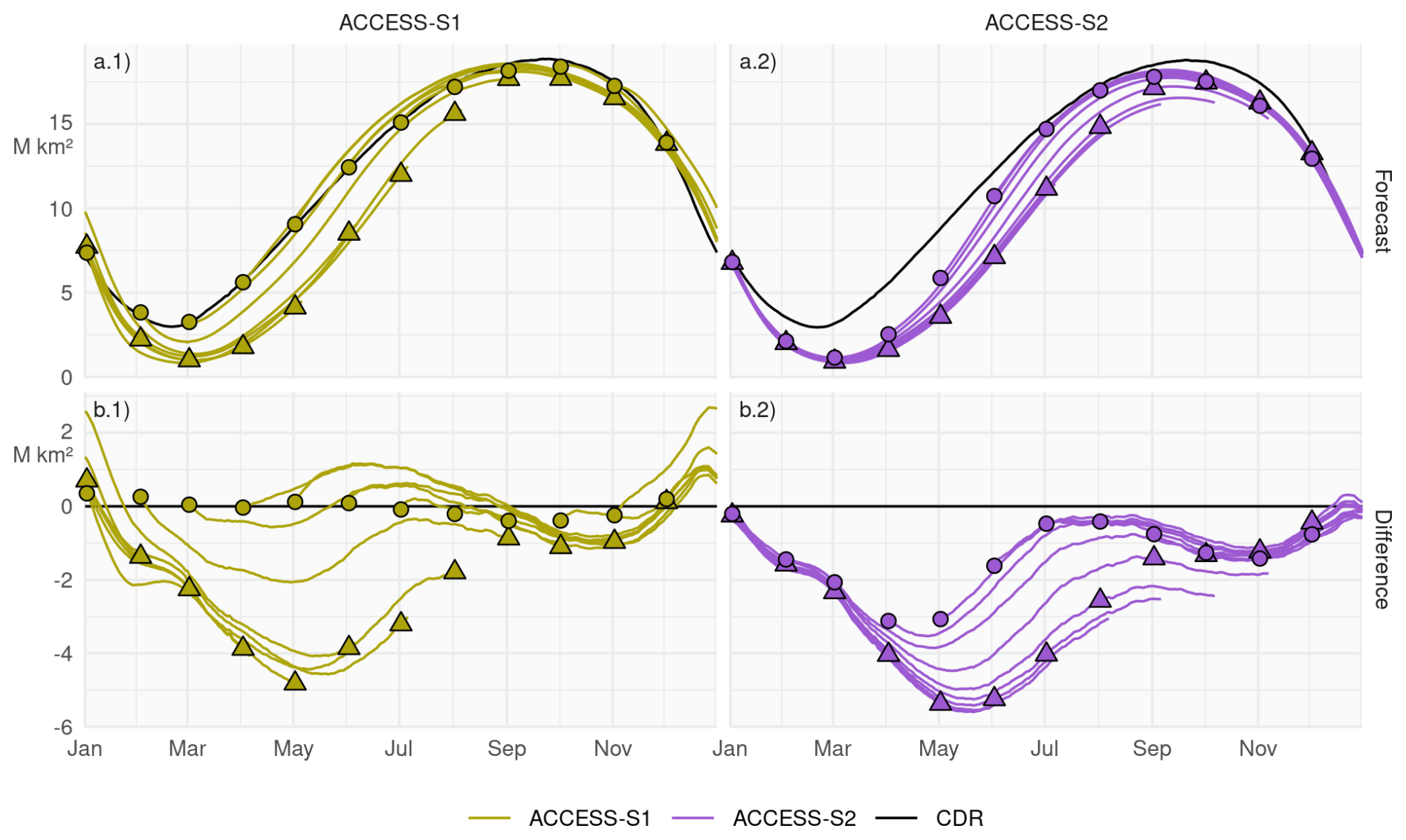
Figure 1 Row (a): Pan-Antarctic daily mean sea-ice extent for all hindcasts initialised on the first of each calendar month for ACCESS-S1 (column 1; green) and ACCESS-S2 (column 2; purple). Observed mean sea-ice extent in each corresponding hindcast period is shown in black. Row (b): Mean differences between the forecast and the observed values. Circles represent the initial conditions at the start of forecasts (i.e., the first of every month), and triangles represent the mean values forecasted for the first of every month at the lead time corresponding to the maximum lead time in S1 (between 213 and 216 d, depending on the month).

ACCESS-S2 initial conditions (circles in Fig. 1 column 2) show an overall negative bias, especially between late summer and early winter, while ACCESS-S1 initial conditions (circles in Fig. 1 column 1) are very close to observations, as expected from the assimilation of sea-ice observations to produce the initial conditions of ACCESS-S1. Both systems' equilibrium states (triangles) show negative biases of sea-ice extent, particularly in the growth phase of late-autumn and winter months. This is due primarily to the melt season being longer in the model than in observations and with faster melt between January and March and the growing seasons being shorter with slower growth during March and April. This is then followed by faster growth between May and July (Figs. 2 and A6). Many sea-ice models exhibit this systematic underestimation during the sea-ice minimum and early freezing season (Bushuk et al., 2021; Massonnet et al., 2023), which could indicate problems in the representation of thermodynamics in the model (Zampieri et al., 2019). It is also not surprising that both forecasting systems converge to a similar equilibrium state because they share the same model formulation.

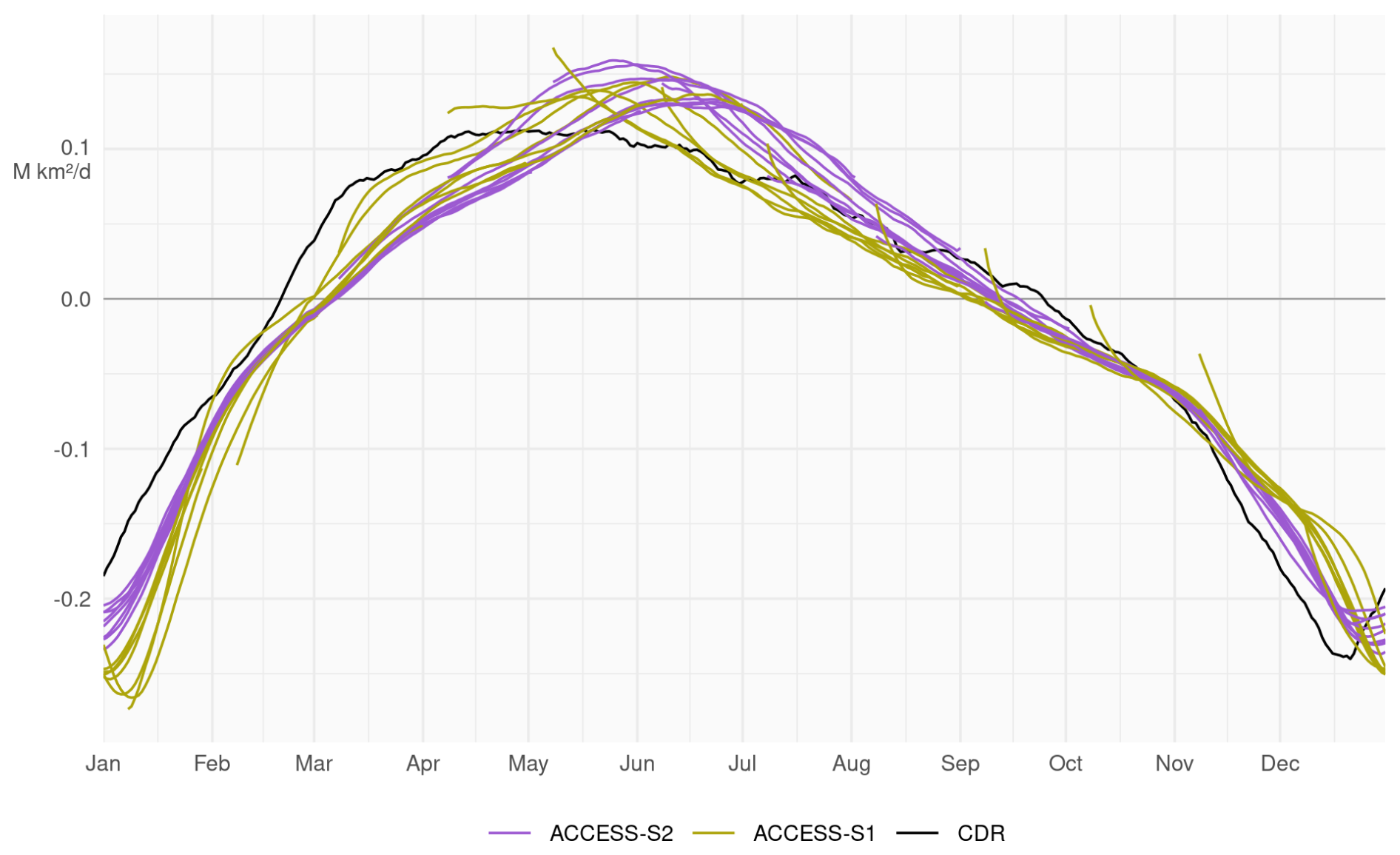
Figure 2 Mean daily sea-ice extent growth (10⁶ km² d⁻¹) in ACCESS-S1 (green) and ACCESS-S2 (purple) hindcasts and observations (black), computed as the mean daily differences in sea-ice extent between each date and the next for each forecast month. Values are smoothed with a 11 d running mean.

The difference between the initial conditions (circles) and the model equilibrium state (triangles) can be mostly attributed to the effect of data assimilation, which in ACCESS-S2 is due solely to the coupling of sea ice with the atmosphere and the ocean. From April to September, in ACCESS-S2, circles are closer to observations than the triangles are, indicating that the information from the ocean and atmosphere data assimilation is affecting sea ice and improving the initial conditions. During these months, ACCESS-S1 can overestimate the sea-ice extent at short lead time. For the rest of the year circles are overlaid with triangles in ACCESS-S2, indicating that the indirect effect of the ocean and atmosphere data assimilation on sea ice is minimal and that this component of the model is virtually free-running.

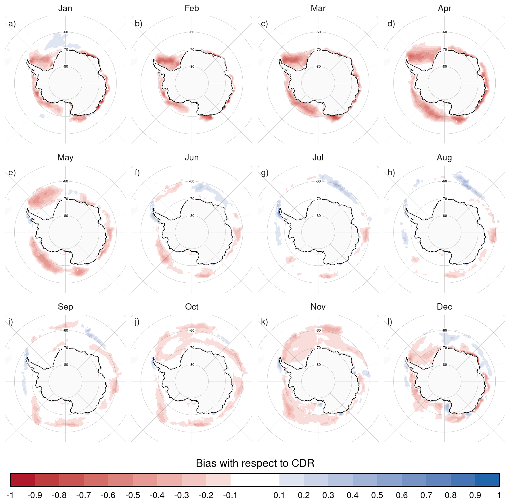
Figure 3 Ensemble mean difference between monthly sea-ice concentration of ACCESS-S2 ensemble mean forecast at 0 month lead time (monthly mean values forecasted from the forecast initialised at the first of the month) and observations (CDR).

To further understand the bias in ACCESS-S2, Fig. 3 (Fig. A7) shows spatial patterns of the differences of monthly mean sea-ice concentrations between NOAA/NSIDC CDRV4 and ACCESS-S2 hindcasts at the shortest monthly lead time. From October to May, the model underestimates sea-ice concentrations in most regions except for the inner Weddell Sea in April and May, where sea-ice concentrations saturate to 1 both in the observations and forecasts. In winter, the differences are limited to a narrow band around the sea-ice edge with slight positive biases in the African sector of East Antarctica and negative biases around the Indian Ocean sector which partially compensate, resulting in the near-zero extent bias seen in those months (Fig. 1).

ACCESS-S1 has a comparatively smaller overall bias (Figs. 4 and A8). The largest values are found between April and June, when the faster growth results in large positive bias along the sea-ice edge, and in January, when the faster melt leads to large negative bias in the Weddell and Amundsen-Bellingshausen Seas.

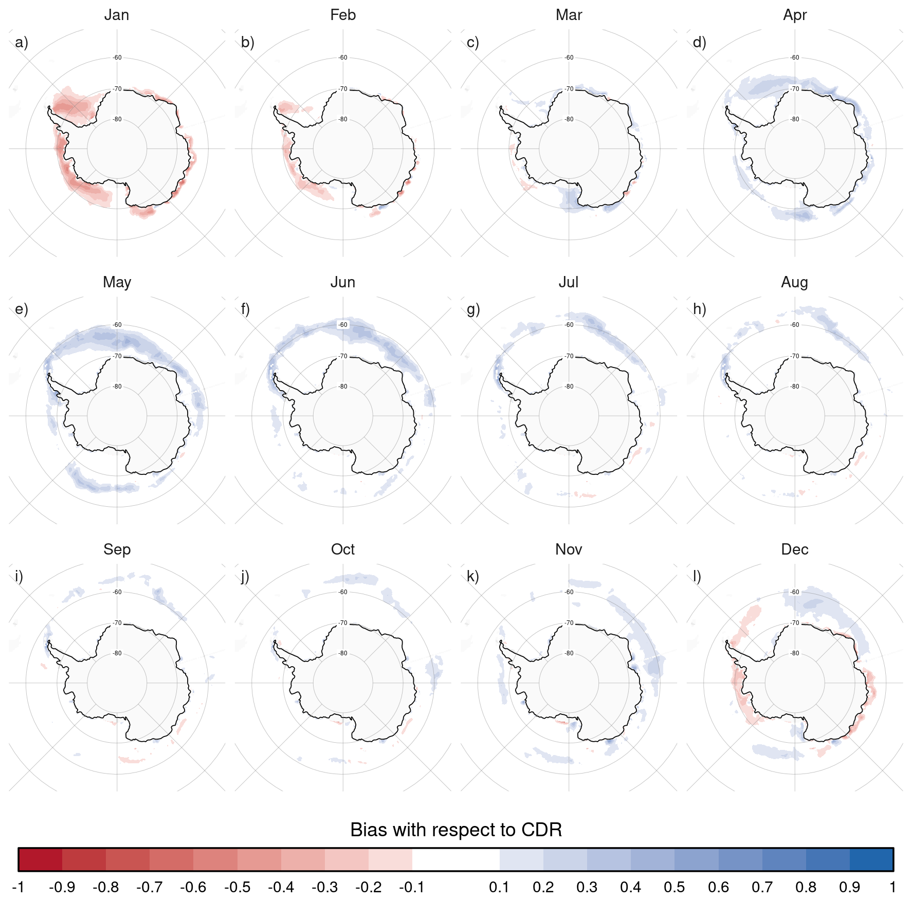
Figure 4 Same as Fig. 3 but for ACCESS-S1.

3.2 Anomaly errors

Figure 5 (Fig. A9) shows monthly sea-ice extent anomalies forecasted at selected lead times. Compared with ACCESS-S1, ACCESS-S2 anomaly forecasts are relatively poor (large RMSE) even for the first month (lead time 0), which is worse than ACCESS-S1 forecasts even at a lead time of six months. ACCESS-S2 shows much larger interannual variability than observations, with dramatic lows between 1995 and 2007, and highs between 2007 and 2015.

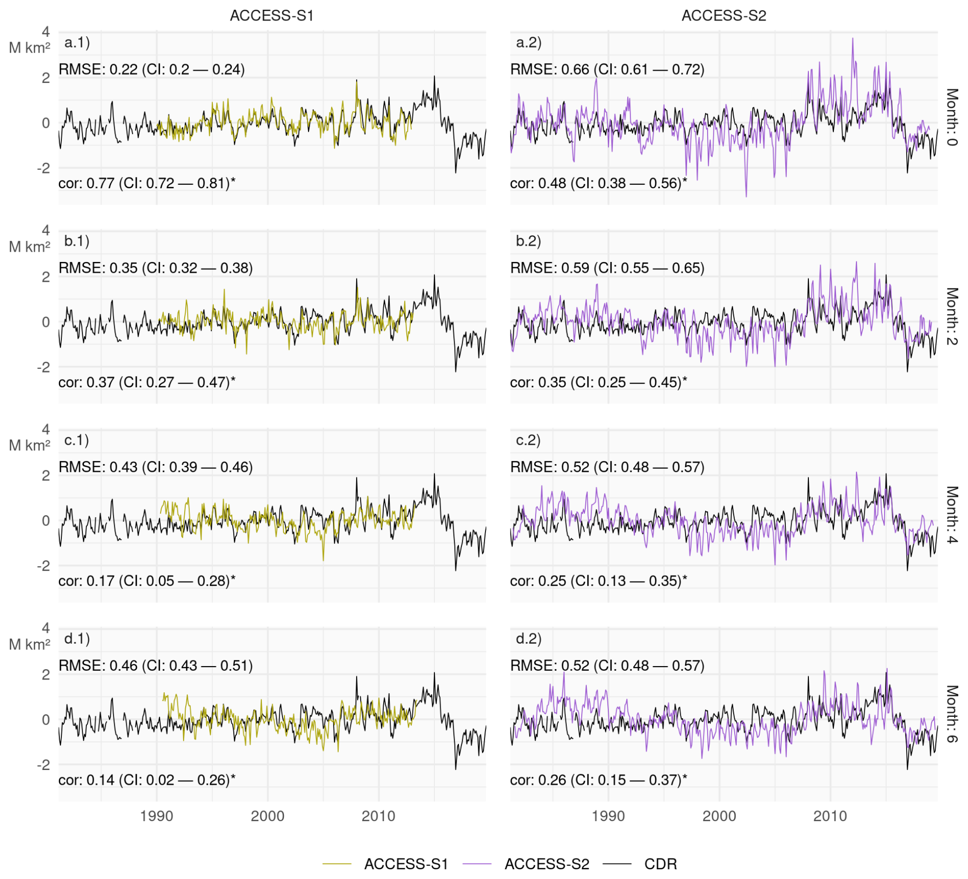
Figure 5 Monthly mean sea-ice extent anomalies of the observations (black) and forecasts from ACCESS-S1 (right column; purple) and ACCESS-S2 (left column; green) at lead times of 0, 2, 4, and 6 months. The RMSE and correlation with their respective 95 % confidence interval during the overlapping period of ACCESS-S1 and ACCESS-S2 hindcasts (1990–2012) are shown on the top left and bottom left of each panel respectively. Statistically significant correlations at 95 % confidence level are marked with an asterisk.

Unexpectedly, for ACCESS-S2, RMSE improves with lead time, even though the correlation degrades with lead time. This effect is seen in all months except from July to September (Fig. A1). This is puzzling behaviour that goes contrary to what is usually seen in prediction models. The explanation seems to be the aforementioned increase in interannual variability. Figure 6 (Fig. A10) shows the interannual standard deviation of monthly sea-ice extent of the forecasts as a function of lead time compared with observations. ACCESS-S1 standard deviation lies within the observed standard deviation regardless of lead time, while ACCESS-S2 standard deviation is more than twice that of observations at zero lead time and only approaches the observed value at nine months lead time for most months.

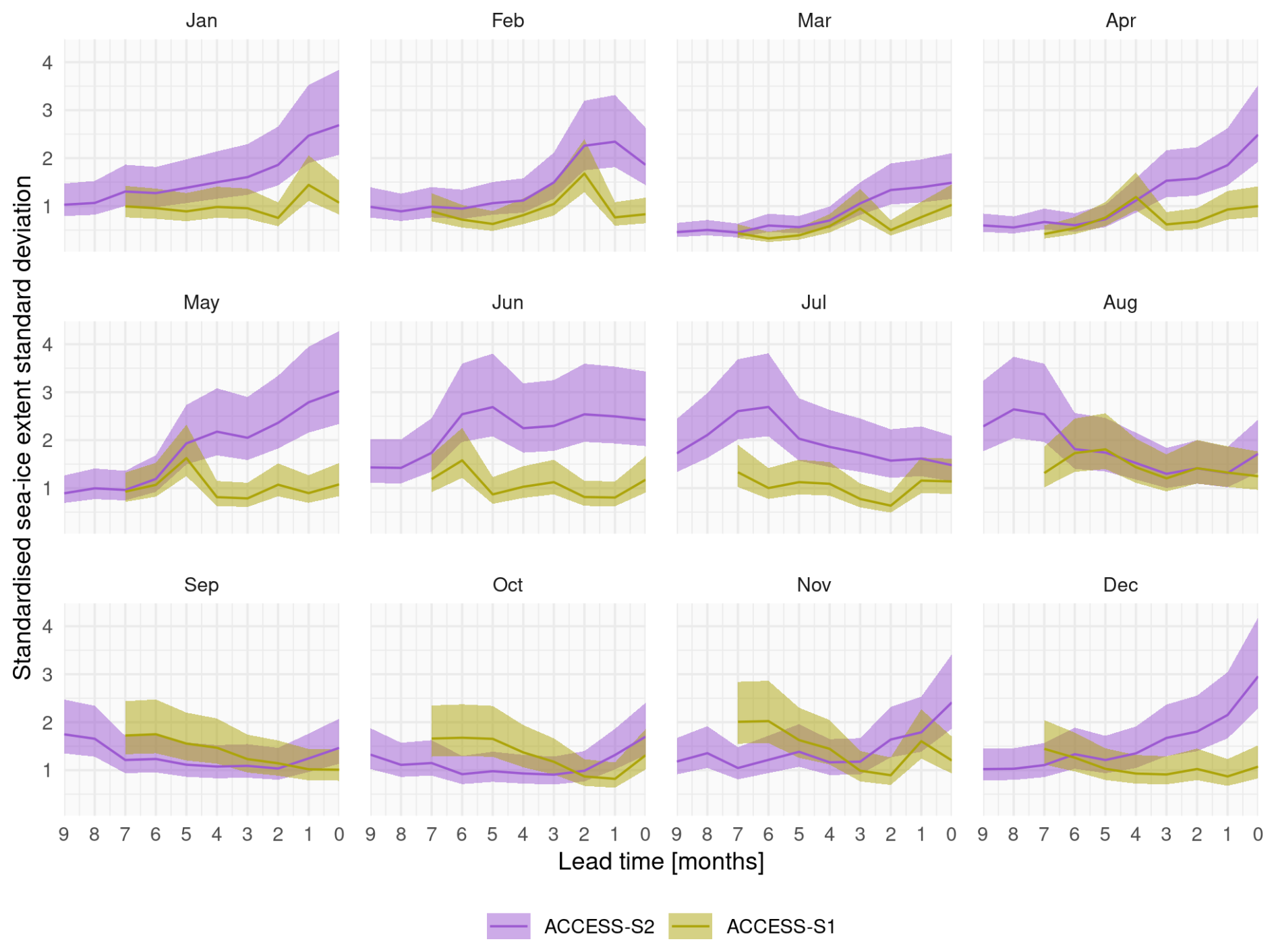
Figure 6 Interannual standard deviation with 95 % confidence interval of monthly mean sea-ice extent forecasted for each month. We standardise the standard deviation by that month's sea-ice extent observation standard deviation. Each panel indicates the target month. Note the reverse horizontal axis.

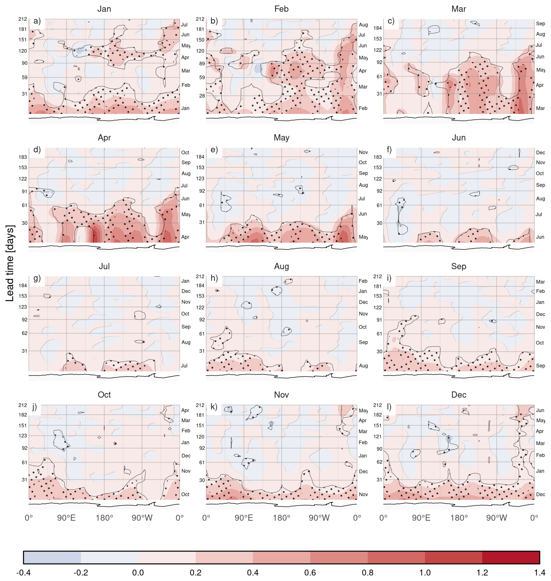
The reason for the increased variability in ACCESS-S2 is not clear. One possible explanation is that ACCESS-S2 simulates thinner sea ice than ACCESS-S1 (Fig. A2 bottom row) that is more sensitive to atmospheric and oceanic forcing. To explore this possibility, Fig. 7 shows the correlation between sea-ice thickness and the magnitude of sea-ice concentration anomalies in the ACCESS-S2 reanalysis. It shows that in most regions and months, thinner ice is correlated with stronger sea-ice concentration anomalies.

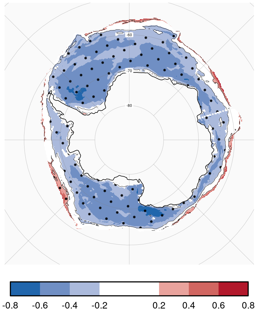
Figure 7 Correlation in the ACCESS-S2 reanalysis between monthly mean sea-ice thickness and the absolute value of monthly mean sea-ice concentration anomalies masked to areas with mean sea-ice concentration greater than 15 % more than 50 % for each month. Regions where the correlation is significant at p-value<0.05 are stipppled.

Figure 8 shows that indeed ACCESS-S2 simulates thinner sea ice compared to ACCESS-S1 overall at almost all lead times and in all months except for summer at short lead times (December–January, 0–1 months; February–March, 0–2 months). However, Fig. 8 also shows that sea-ice thickness tends to decrease at longer lead times, when ACCESS-S2's variability converges to observed variability. Furthermore, the thickness difference between ACCESS-S1 and ACCESS-S2 is large also in months in which ACCESS-S2 sea-ice extent variability is comparable to ACCESS-S1 and where ACCESS-S2's RMSE does not decrease with lead time, such as August and September.

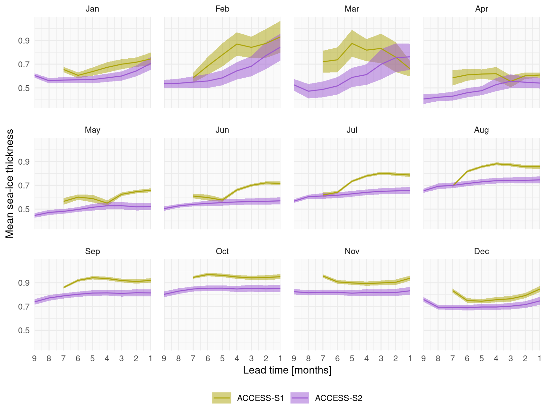
Figure 8 Mean and 95 % interval of monthly mean sea-ice thickness for ACCESS-S1 and ACCESS-S2 at different lead times. Each panel indicates the target month. Note the reverse horizontal axis.

Even if ACCESS-S2's sea ice is more sensitive to atmospheric and oceanic forcings than ACCESS-S1 by being overall thinner, this is not a sufficient explanation for the pattern of increased variability at shorter lead times and its absence in particular months. Instead, the strengths of the atmospheric and oceanic forcings might also be playing a role. The fact that ACCESS-S1 and ACCESS-S2 share the same model configuration and that the increased variability is more extreme at short lead times (Fig. 6) suggests that the data assimilation procedure might also be partly responsible. We speculate that it is possible that sea ice in the ACCESS-S2 system is left in an unbalanced state by assimilating atmospheric and oceanic data but not sea-ice data, leading to large responses that are amplified by the thinner ice. Teasing this out would require an in-depth analysis of the data assimilation innovations, which is out of scope for this work.

To assess ACCESS-S2 forecasts in more detail, we compute error measures for all hindcasts started on the first of every month. Figure 9 (Fig. A11) shows the mean RMSE of sea-ice concentration anomalies for ACCESS-S1 and ACCESS-S2 hindcasts compared against persistence and climatological forecasts used as a benchmark. Due to errors in the initial conditions, it is expected that persistence forecasts would be better than the model forecasts at very short lead times, but that the persistence forecast errors would grow faster and may eventually surpass the model forecast errors. The black line shows that the persistence forecast error indeed grows rapidly and reaches its maximum in about 30 d for most months except for February, when it grows much slower. The ACCESS-S1 forecast errors grow slower than persistence forecast errors and remain lower after less than 10 d on average. The ACCESS-S2 forecast error starts high in all months and is lower than the persistence forecast error after more than 15 d in most months except for forecast initialised in February, when it takes 80 d.

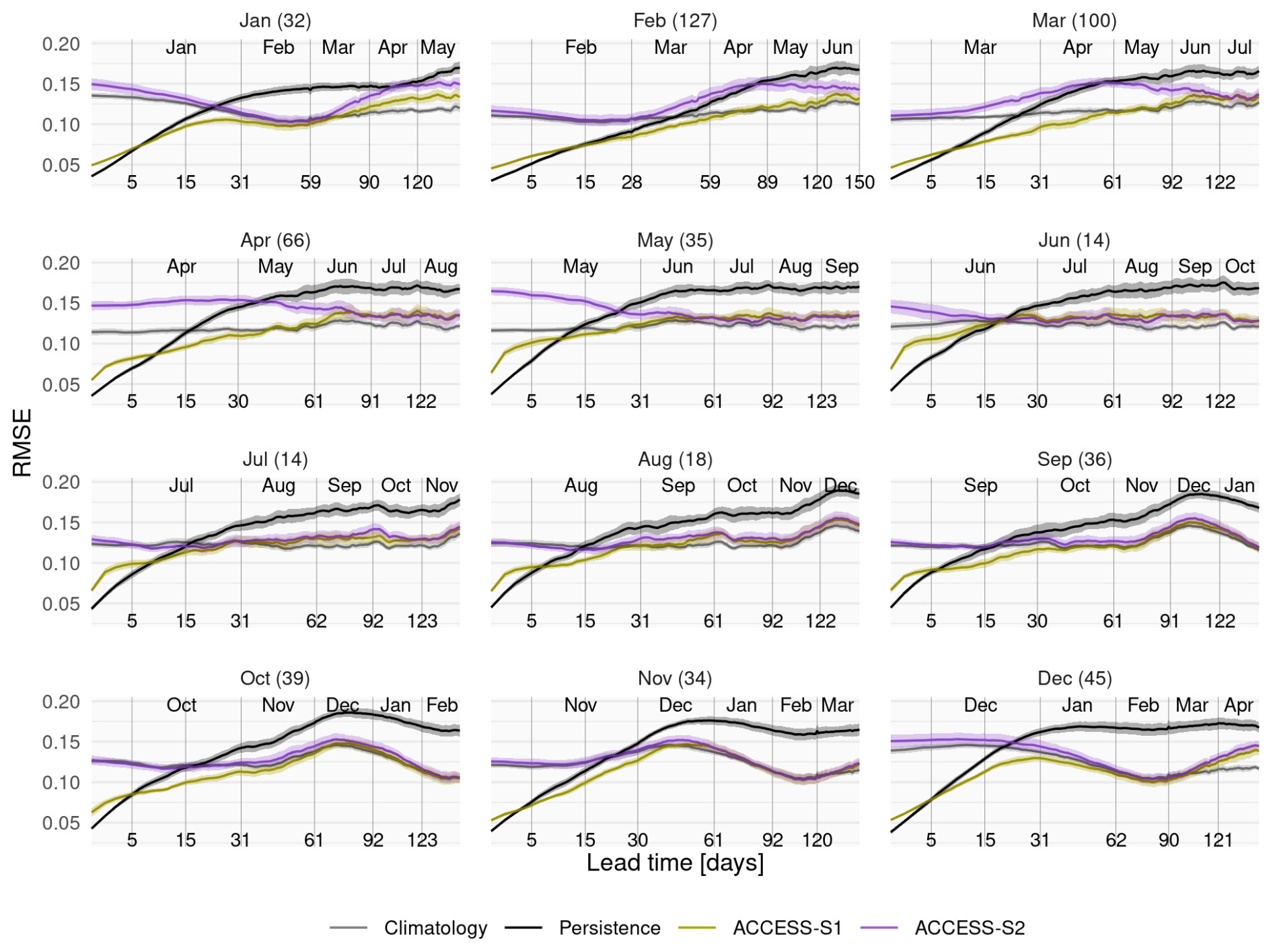
Figure 9 Mean RMSE of sea-ice concentration anomalies as a function of forecast lead time for all forecasts initialised on the first of each month compared with a reference forecast of persistence of anomalies (black) and climatology (gray). The shading indicates the 95 % confidence interval of the mean. Only the first 150 d are shown. In parentheses, the shortest time at which ACCESS-S1 and ACCESS-S2 mean RMSE is not statistically different at the 99 % confidence level. Note that the horizontal axis uses a square root transformation to expand the shorter lead times.

At longer lead times, it is more appropriate to compare errors with the climatological forecast error. The lead time at which ACCESS-S1 forecast error is higher than the climatological forecast error varies between more than 60 d and less than 20 d depending on forecast initialisation month with the minimum length in June. ACCESS-S2 forecasts never have lower error than climatology, on the other hand, except marginally in October forecasts.

In summary, ACCESS-S1 forecasts have a longer lead time in which it is skillful in the summer than the other seasons. Forecasts initialised between May and July are particularly poor, and June cannot be forecasted better than the benchmarks, suggesting a winter barrier in predictive skill (Fig. A3). This is similar to the mid-winter loss of predictability observed by Libera et al. (2022) for the Weddell Sea, who attributed it to deep warm water entraining into the mixed layer.

We quantify the skill difference between ACCESS-S1 and ACCESS-S2 in Fig. 10 by computing the shortest lead time in which the mean RMSE of each system's forecast are not statistically different. The median difference is around 35 d but the biggest difference is between February and April, where ACCESS-S1 forecasts have lower RMSE than ACCESS-S2's for more between 65 and 125 d. The smallest difference, on the other hand, is in winter, when ACCESS-S1's forecast are statistically indistinguishable from ACCESS-S2's after less than 20 d. Assimilation of sea-ice concentration data seems to have a much greater effect in the late summer than in the winter.

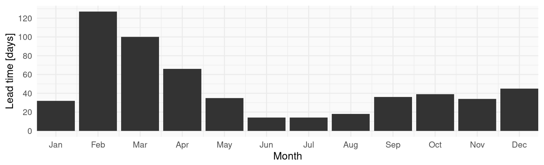
Figure 10 Shortest lead time at which ACCESS-S1 and ACCESS-S2 mean RMSE is not statistically different at the 99 % confidence level.

To analyse the spatial distribution of the model error, we computed the RMSE of zonal mean sea-ice concentration anomalies on 15 slices of 24° longitude span for each forecasting system. We control for some areas being naturally easier to forecast than others by computing the RMSE skill score with the climatological forecast RMSE as reference.

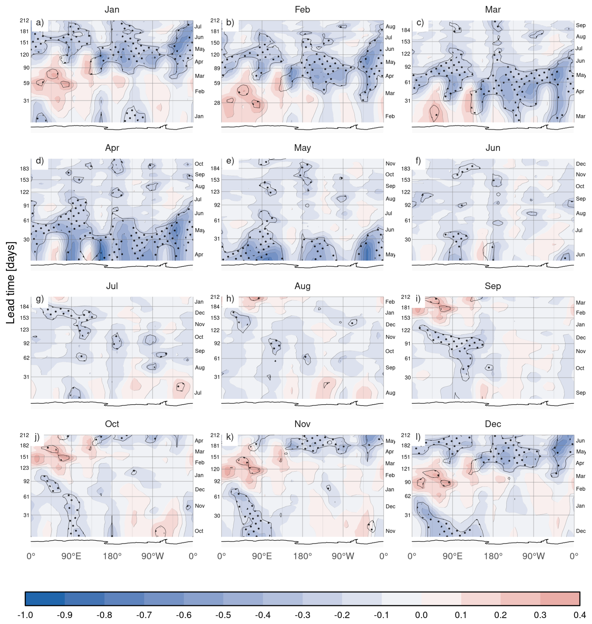
For ACCESS-S1 forecasts (Figs. 11 and A12), skill tends to be lower off the coast of East Antarctica even at short lead times. This is particularly important for forecasts initialised between May and July, where we see that the low skill in early winter (Figs. 9 and A3) is only a feature in East Antarctica where skill is even negative at almost zero lead time. ACCESS-S1 forecasts have relatively high predictive skill in the Weddell Sea in winter, consistent with other seasonal prediction systems (Bushuk et al., 2021). July forecasts have positive (albeit not statistically significant) skill with hindcasts initialised as early as February. The winter predictive skill barrier thus seems to come in great part from large errors in East Antarctica.

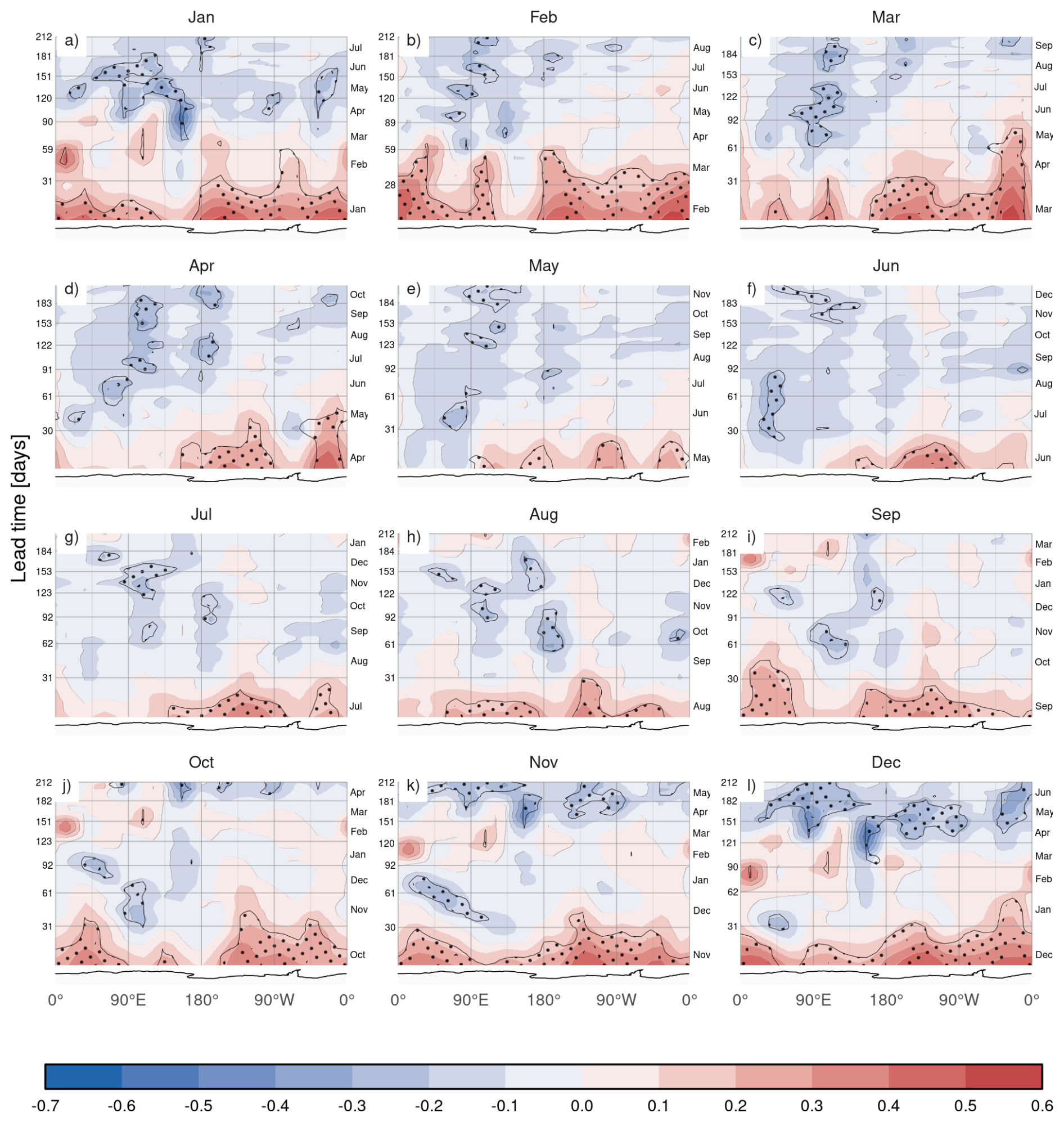
Figure 11 MSE skill score of ACCESS-S1 forecasts with climatological forecast as reference computed on 15 meridional slices 24° wide as a function of lead time and longitude. Regions where the difference of means between ACCESS-S1 RMSE and climatological RMSE are significant at p-value<0.05 are stipppled. Antarctica's coastline is shown at the bottom of each panel for reference. Values were smoothed with an 11 d running mean to improve readability. Note that the vertical axis uses a 1.5 root transformation to expand the shorter lead times.

In West Antarctica there is a hint of easterly-propagating skill in forecasts initialised in February and March. This is consistent with Holland et al. (2013), who found that the memory of sea-ice anomalies is stored in ocean heat content anomalies that are transported eastwards by the Antarctic Circumpolar Current.

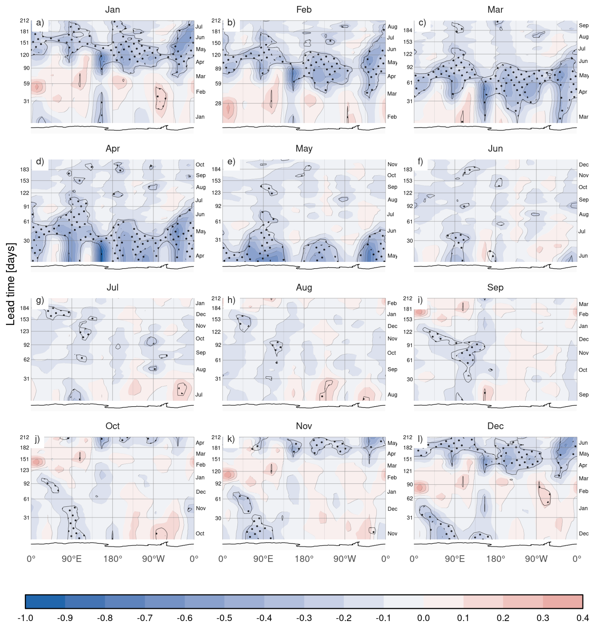
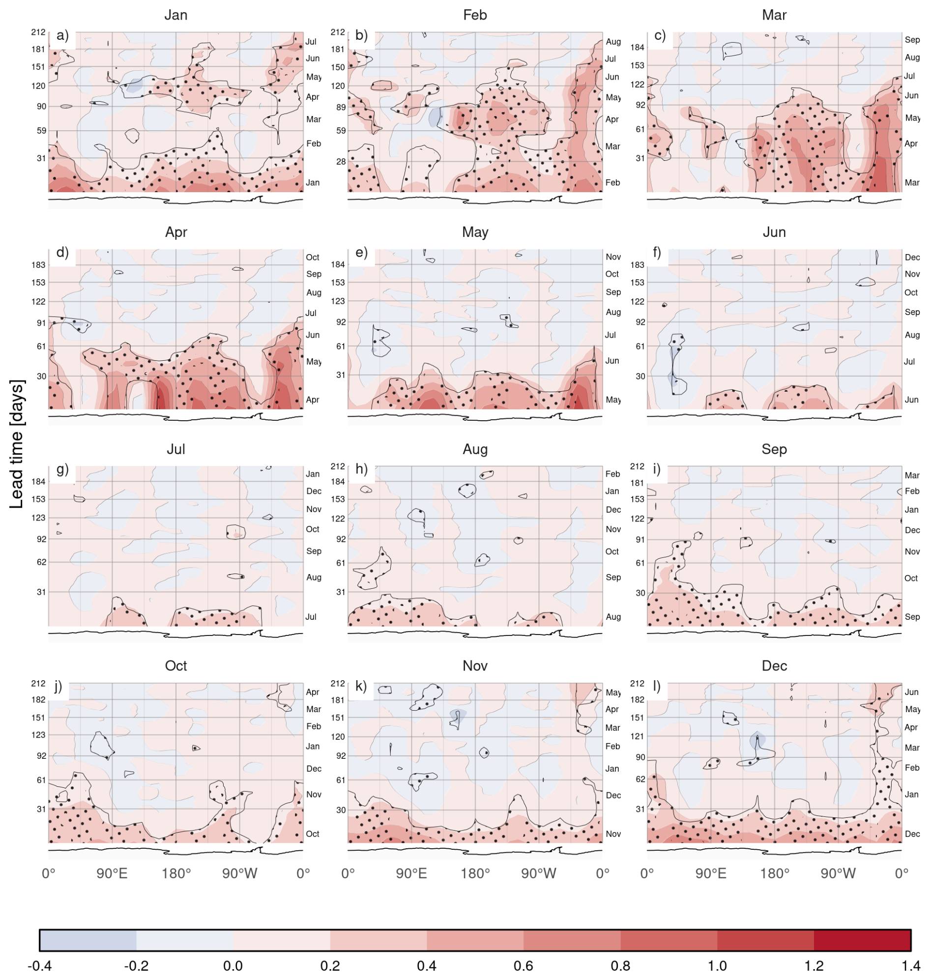
ACCESS-S2 forecasts (Figs. 12 and A13) also have lower skill over East Antarctica. From July to December, even though the pan-Antarctic average skill is negative at all lead times (Fig. A3), it is positive (but not statistically significant) for up to a month in West Antarctic. Since oceanic and atmospheric forcings provide the only source of observational information, this suggests that sea ice in this region is particularly sensitive to oceanic and atmospheric forcing. The fact that this is evident in the months in which El Niño–Southern Oscillation teleconnections via the Pacific-South American mode and the Amundsen Sea Low are more important for atmospheric circulation (Mo and Paegle, 2001; Clem and Fogt, 2013; Wang et al., 2023) also suggests the influence of tropical Pacific variability. February and March are the only two months that can be forecasted with marginally positive skill in large regions.

Figure 12 Same as Fig. 11 but for ACCESS-S2.

Finally, Fig. 13 (Fig. A14) shows the difference in skill between ACCESS-S1 and ACCESS-S2. Large differences in skill indicate areas and months that are most affected by the data assimilation present in ACCESS-S1. Between January and March, when ACCESS-S1 is the most skillful (Fig. A3), most of the higher skill compared with ACCESS-S2 is present in the Ross and Weddell Seas. In April and May, the higher skill seems more homogeneous. In June and July, ACCESS-S1 has higher skill only at very short lead times and in limited regions; in particular we see that in June there is no skill difference in the King Haakon Sea – between 0 and 90° E.

Figure 13 Same as Fig. 11 but for the difference between ACCESS-S1 and ACCESS-S2.

3.3 Limitations

This analysis rests on the assumption that the main difference between ACCESS-S1 and ACCESS-S2 is the lack of data assimilation of sea-ice concentrations. However, although both systems use the same model configuration and atmospheric initial conditions, they also differ in the ensemble generation scheme and their ocean initial conditions.

As mentioned in Sect. 2.1, ACCESS-S1 ensemble members are generated by adding random field perturbations to the atmosphere only, which then are transferred to the other components via the coupled simulation (Hudson et al., 2017) while ACCESS-S2 ensemble members are generated by time-lagged ensemble.

We believe this difference would only alter the ensemble spread and should have minimal impact in the dramatic differences in ensemble mean error shown in Fig. 9. In ACCESS-S1's scheme, ensemble members are all but guaranteed to be underdispersed in the ocean and sea-ice components. To test the effect of the ensemble generation scheme on ensemble spread, we compute the mean variance of RMSE of individual forecasts as a function of lag for each forecasting system. Figure A4 shows that indeed ACCESS-S1's initial spread is much lower than ACCESS-S2's in every month. However, ACCESS-S1's ensemble spread grows quickly, and after less than a week, both systems' spread is comparable. For forecasts initialised in February, March and April, ACCESS-S1 even has larger spread than ACCESS-S2.

Regarding ocean initial conditions, unfortunately we cannot directly compare ACCESS-S1 and ACCESS-S2 initial conditions because those data are currently not available. However, we believe there are reasons to consider that the effect would be of second-order importance. While the ocean data assimilation process is different, the underlying observations are similar, especially in the high latitudes, where there are few direct observations in total.

As an indirect comparison of ocean initial conditions, Wedd et al. (2022) in their Fig. 9 show the correlation of ocean heat content in the upper 300 m of the ocean between EN4 and ACCESS-S2 and ACCESS-S1 reanalysis. In both systems, correlations are relatively high around 60° S and very low in the Antarctic coast; importantly, their correlation patterns are very similar, suggesting that the ocean initial conditions are not too dissimilar between the two systems. A limitation of this comparison is that the low correlation seen in both systems in the ice-covered regions only indicates that both systems have poor ocean initial conditions in that region but does not necessarily mean that their initial conditions are similar. Even though the ocean initial conditions are similarly correlated with the reference dataset in both systems, SST forecasts were shown by Wedd et al. (2022) to be highly degraded in the Southern Ocean even at zero months lead time in ACCESS-S2 compared with ACCESS-S1. Correlation of SST anomalies in the ice-covered regions is much lower for ACCESS-S2 (Wedd et al., 2022, Fig. 13) and with a higher positive bias (their Fig. 12), which is consistent with the greater negative sea-ice concentration bias in ACCESS-S2 (Fig. 1). This raises the possibility that it is the lack of assimilation of sea-ice data that is degrading SST forecasts and not the other way around.

4 Conclusions

Sea-ice forecasts from the ACCESS-S2 system show a significant low extent bias, particularly during late summer and early autumn. This bias is attributed to a faster and longer melt season between January and March, and slower growth between March and April. This underestimation during the minimum and early freezing season is a common issue in many subseasonal-to-seasonal systems, suggesting potential problems either with the model's thermodynamic representation or with short wave radiation forcing, as shown in other climate models (Zampieri et al., 2019; Roach et al., 2020). Even though ACCESS-S2 shares the same model components as ACCESS-S1, the latter does not suffer from this bias, indicating that assimilating sea-ice concentrations successfully corrects for the negative bias that exists in the free-running model.

Ensemble spread grows quickly even when perturbations are only implemented in the atmosphere component (in ACCESS-S1), indicating that sea ice is indeed responding quickly to atmospheric perturbations. However, our analysis suggests that the atmosphere and ocean data assimilation implemented in ACCESS-S2 is only effectively influencing sea-ice initial conditions from June to October, while the rest of the year, the sea-ice component runs virtually free, reverting to its biased equilibrium state. Zhou and Alves (2022) had previously evaluated sea-ice forecasts in ACCESS-S2 and also highlighted the poor performance of this forecasting system attributed to the lack of good initial conditions.

Although ACCESS-S1 only assimilates sea-ice concentration, it is clear that sea-ice thickness is also affected through the assimilation process. ACCESS-S1 simulates significantly thicker ice than ACCESS-S2 and in both systems sea ice is thicker at shorter lead times than at longer lead times. Both the explicit data assimilation in ACCESS-S2 and the effects of atmospheric and oceanic data assimilation in ACCESS-S1 might be nudging simulated sea ice to be thicker than the model equilibrium state. It still remains unclear why ACCESS-S2 simulates much larger interannual variability than ACCESS-S1 at shorter lead times. We suggest that the thinner sea ice in ACCESS-S2 contributes to the large sea-ice extent variance, but other mechanisms, such as unbalanced initial conditions might also be important.

Given that ACCESS-S2 sea-ice extent is not directly initialised by sea-ice observations, and assuming that the effects of the slightly different ocean initial conditions and ensemble generation are of second-order importance, comparing its forecasts with those of ACCESS-S1 allows us to estimate the time-scale over which initial conditions are important. We find that initial conditions affect Antarctic sea-ice forecasts on the order of a few months, but that effect is seasonally dependent. January to April initial conditions improve forecasts for up to three months. February initial conditions in particular are shown to be crucial for determining sea-ice evolution at least up to May. Arctic sea-ice forecasts also show greater sensitivity to initial conditions in boreal summer, compared with boreal winter (Day et al., 2014; Bunzel et al., 2016), suggesting a similar mechanism might be playing a role.

These results contrast with Xiu et al. (2025), which used a very similar methodology to our own. Based on their claims that assimilation of sea-ice concentration data doesn't improve sea-ice forecasts compared with only assimilating ocean data and that atmospheric conditions are enough for a skillful sea-ice forecast, we would have expected skillful forecasts from ACCESS-S2's atmosphere initial conditions. It is possible that model biases are important to explain this discrepancy. Their forecasting system simulated more sea ice than observations; the reverse of ACCESS-S1 and ACCESS-S2, which tended to drift into lower sea-ice concentration that needed to be corrected with data assimilation. However, since they used anomaly field assimilation, which assimilates anomalies on top of the model's own climatology, their initial conditions were close to the model's own equilibrium state, reducing the strong initial shock of the type we detected in ACCESS-S1 and which we speculate might be degrading variability in ACCESS-S2.

Forecasts initialised in the winter have very little skill and ACCESS-S1 and ACCESS-S2 forecast errors are statistically indistinguishable after just two weeks. Contrasting to Libera et al. (2022) but consistent with Xiu et al. (2025), we find that this predictive skill barrier is not apparent in the Weddell Sea and instead comes from low skill in the Indian Ocean sector. However, we cannot make a direct comparison between Libera et al. (2022) and our study due to significant methodological differences. Their results were based on persistence of sea-ice area, whereas here we study errors in sea-ice concentration anomalies of a dynamical model. Further exploration of these differences could lead to more insight in how persistence-based measures of predictability translate to actual predictive skill.

These findings have important implications for both operational forecasting, model development and predictability studies. For operational centers, our results suggest that efforts to improve sea-ice data assimilation should prioritize the summer and autumn months when initial conditions have the greatest impact on forecast skill. Additionally, the substantial bias in both models highlights the need for improved model physics, particularly in the representation of sea-ice thermodynamics and radiation processes. Crucially, our results suggest dramatic seasonal variations in sea-ice predictability. Predictability studies should therefore sample initial conditions throughout the whole year instead of focusing on a limited number of initialisation dates. Our conclusions are limited by the fact that ACCESS-S1 and ACCESS-S2 also differ in the ocean data assimilation system and the ensemble generation method. Although we believe these differences to be of second-order importance compared with the wildly divergent sea-ice initial conditions, we cannot rigorously discard nor directly quantify their influence; these issues motivate the need for more targeted experiments.

Appendix A

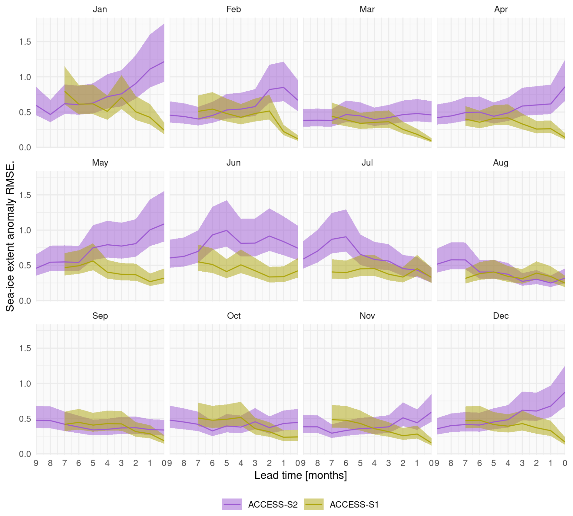
Figure A1 RMSE of monthly mean sea-ice extent anomalies as a function of lead time (months) for ACCESS-S1 (green) and ACCESS-S2 (purple). RMSE is computed over the overlapping period of ACCESS-S1 and ACCESS-S2 hindcasts (1990–2013). Each panel indicates the target month. Note the reverse horizontal axis.

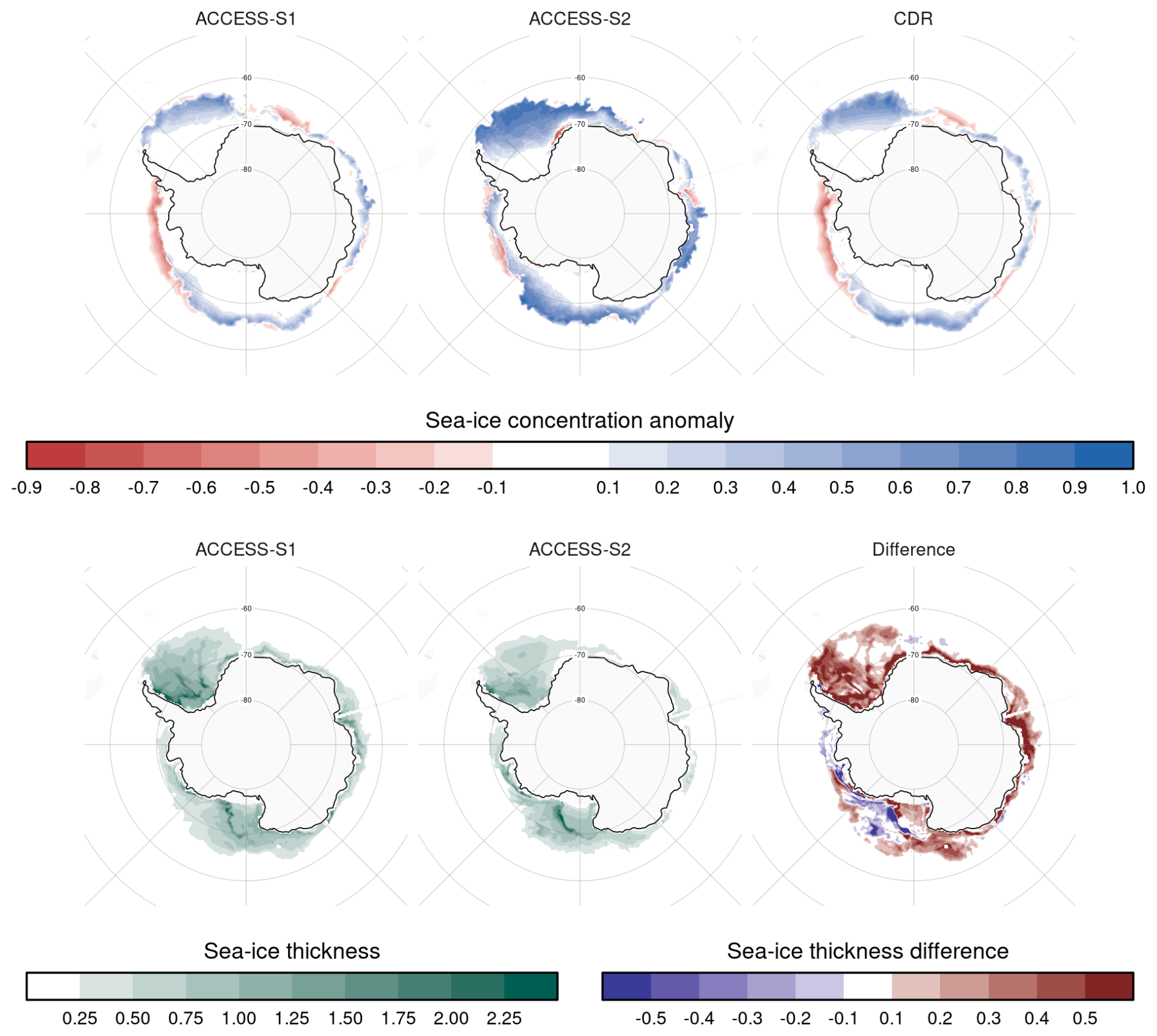
Figure A2 ACCESS-S1 and ACCESS-S2 hindcasts for 2 May 2008 at one day lead time. Top row shows sea-ice concentration anomalies forecasted by each system and the observations. Bottom row shows forecasted sea-ice thickness and the difference between ACCESS-S1 and ACCESS-S2. ACCESS-S2 simulates large sea-ice concentration anomalies in the Weddell and Ross Seas and slight negative anomalies in the Amundsen and Bellingshausen Seas that align fairly well with observations, but the magnitude of the anomalies is too big. ACCESS-S1's sea-ice concentration anomalies are close to observations. At the same time, ACCESS-S2 simulates thinner ice than ACCESS-S1.

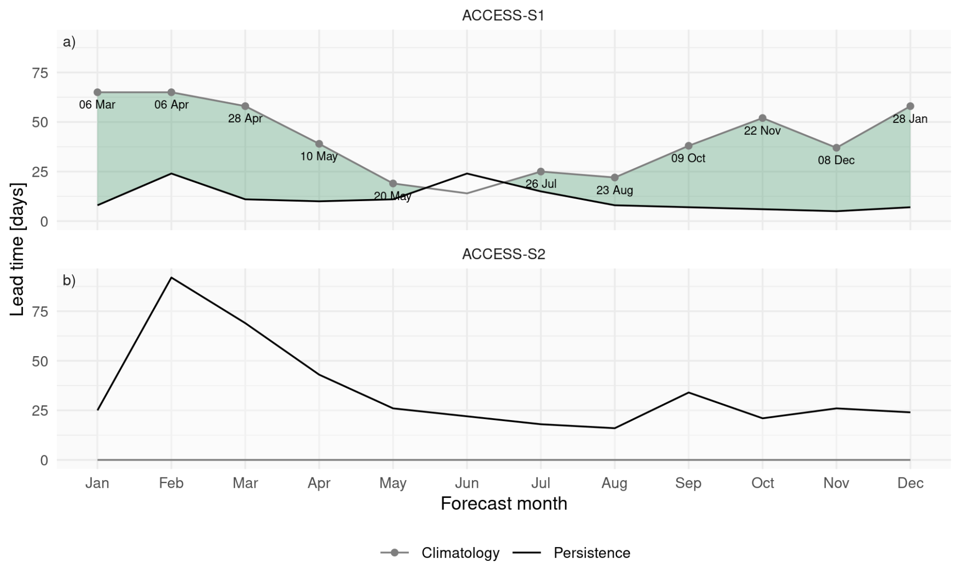
Figure A3 Minimum lead time at which each forecast's mean RMSE becomes lower than the lower bound of the 95 % confidence interval of persistence forecast RMSE (black lines) and maximum lead time at which each forecast's mean RMSE remains lower than the lower bound of the 95 % confidence interval of climatological forecast RMSE (gray lines). Green shading indicates the window where forecasts outperform both persistence (lead times longer than black line) and climatology (lead times shorter than gray line). Text labels show the date corresponding to the maximum lead time at which each forecast outperforms climatology. Using CDR as the validation dataset.

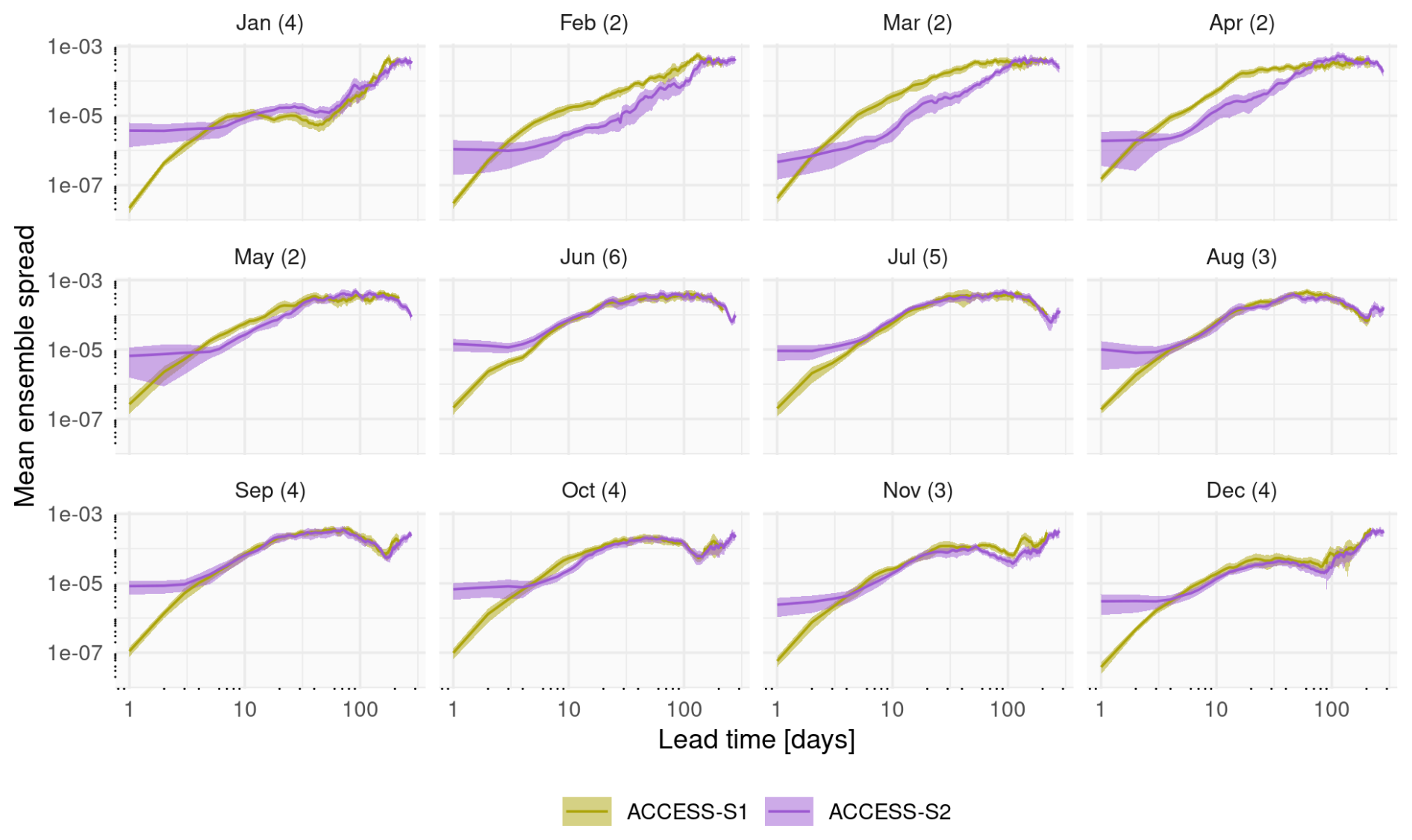
Figure A4 Mean variance of RMSE between ensemble members of each forecast. In parentheses, the shortest minimum lead time at which ACCESS-S1 mean spread becomes larger than the lower bound of the 95 % confidence interval of ACCESS-S2 spread. Note the double log scale.

The following are the same figures from the main paper but using the OSI dataset instead of CDR.

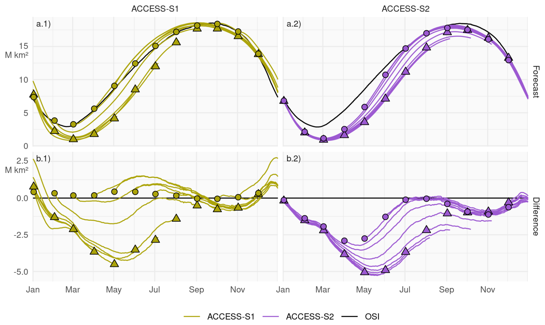
Figure A5 Row (a): Pan-Antarctic daily mean sea-ice extent for all hindcasts initialised on the first of each calendar month for ACCESS-S1 (column 1; green) and ACCESS-S2 (column 2; purple). Observed mean sea-ice extent in each corresponding hindcast period is shown in black. Row (b): Mean differences between the forecast and the observed values. Circles represent the initial conditions at the start of forecasts (i.e., the first of every month), and triangles represent the mean values forecasted for the first of every month at the lead time corresponding to the maximum lead time in S1 (between 213 and 216 d, depending on the month).

Figure A6 Mean daily sea-ice extent growth (10⁶ km² d⁻¹) in ACCESS-S1 (green) and ACCESS-S2 (purple) hindcasts and observations (black), computed as the mean daily differences in sea-ice extent between each date and the next for each forecast month. Values are smoothed with a 11 d running mean.

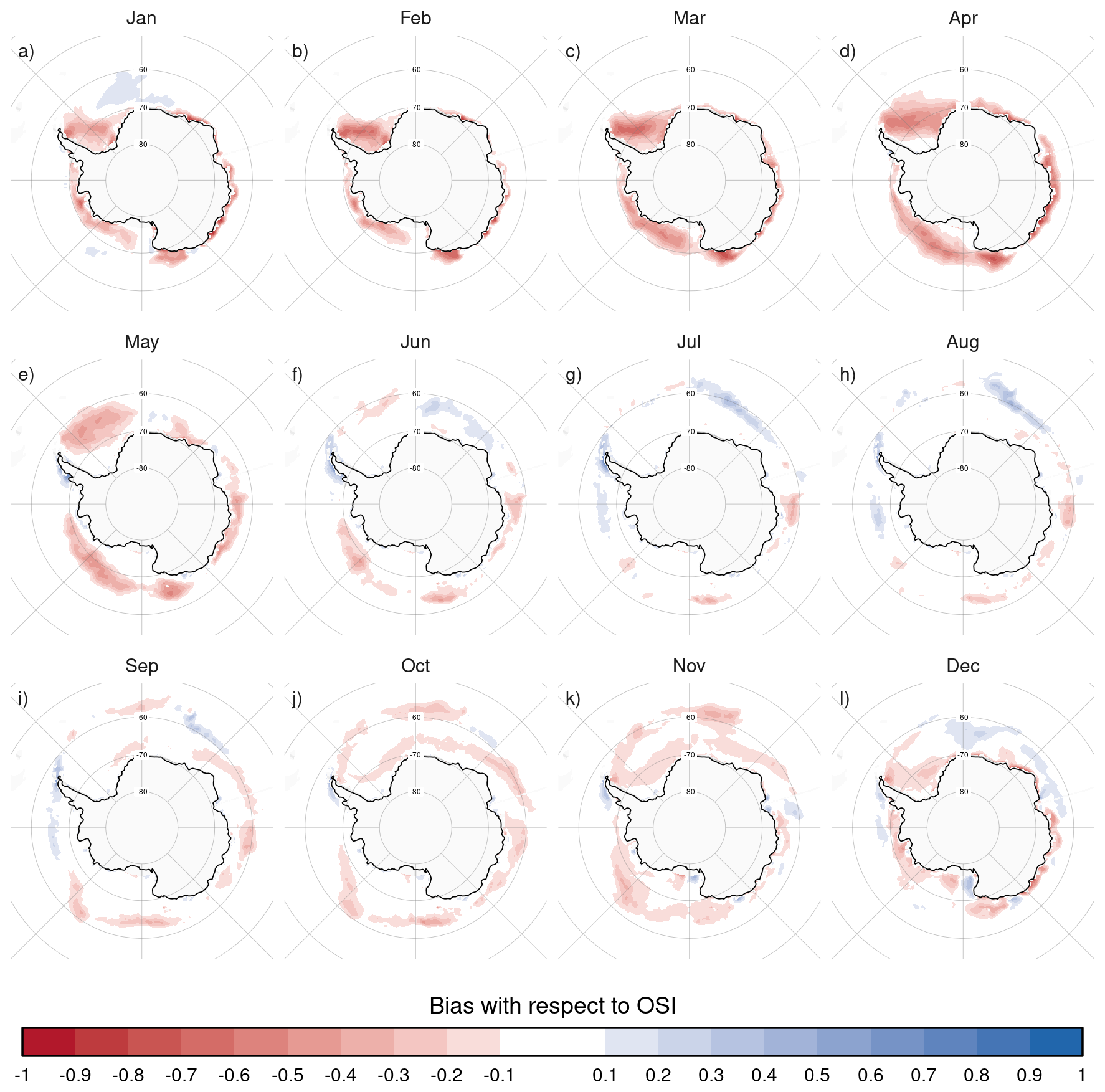
Figure A7 Ensemble mean difference between monthly sea-ice concentration of ACCESS-S2 ensemble mean forecast at 0 month lead time (monthly mean values forecasted from the forecast initialised at the first of the month) and observations (OSI).

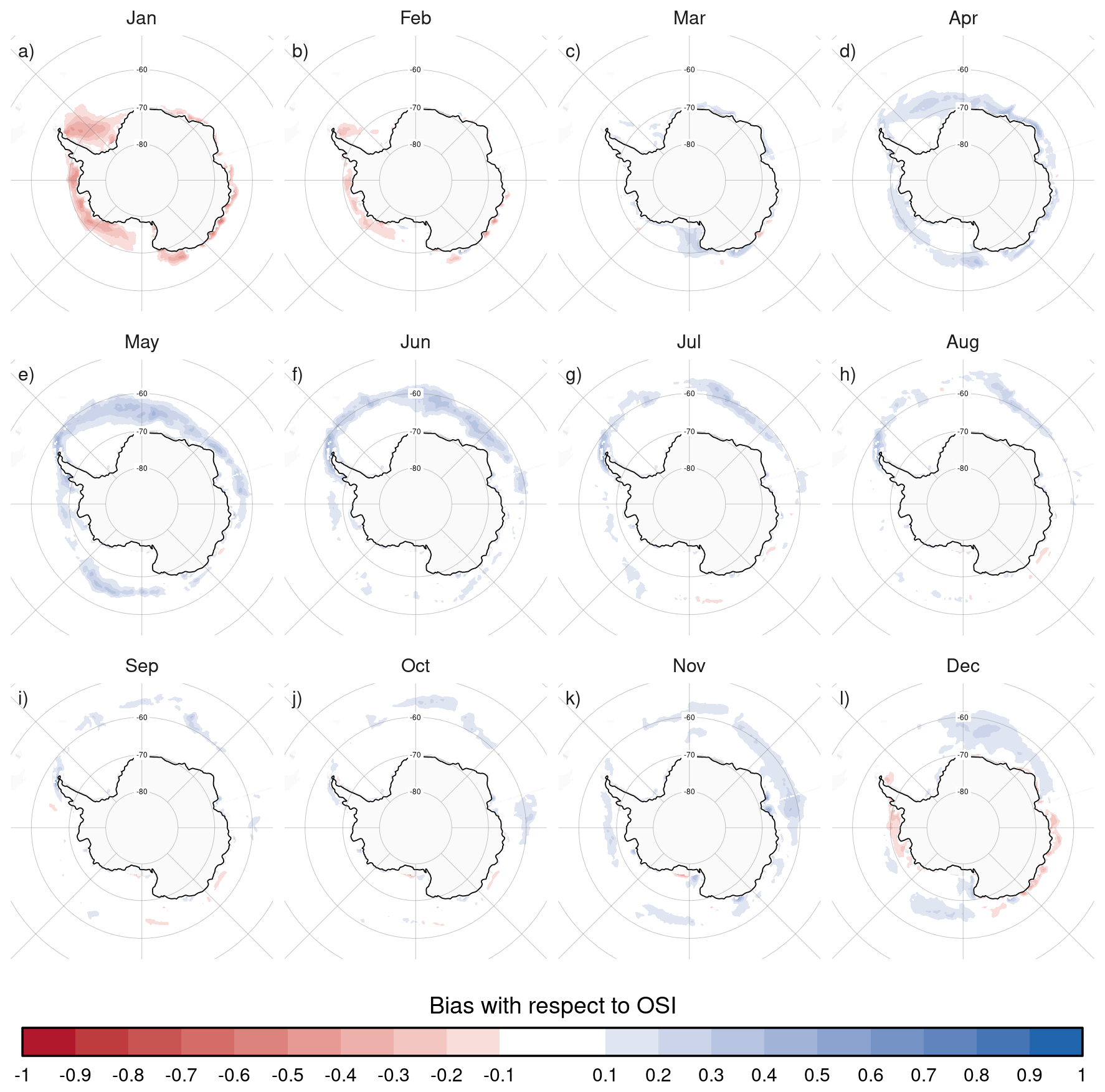
Figure A8 Same as Fig. 3 but for ACCESS-S1.

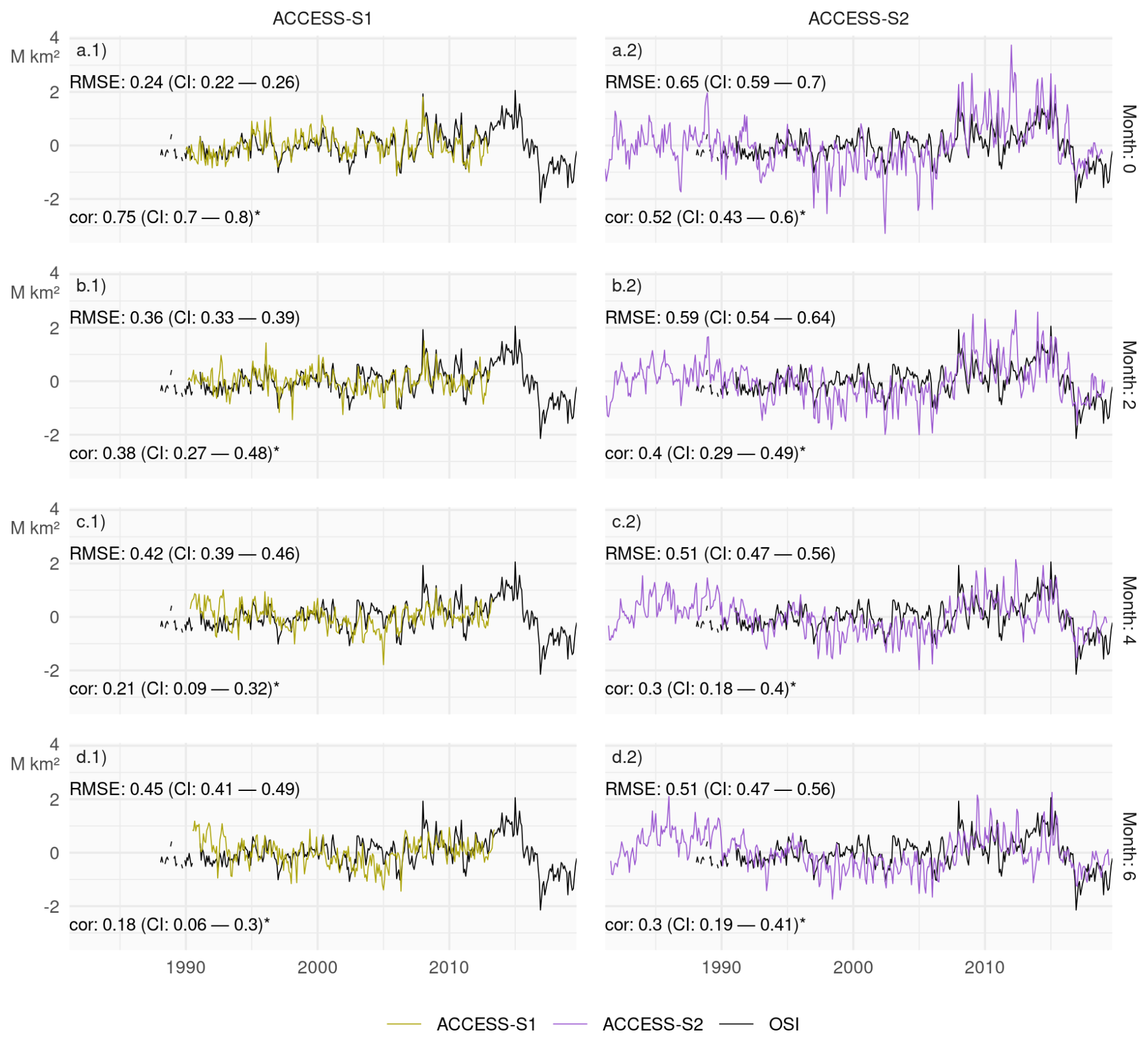
Figure A9 Monthly mean sea-ice extent anomalies of the observations (black) and forecasts from ACCESS-S1 (right column; purple) and ACCESS-S2 (left column; green) at lead times of 0, 2, 4, and 6 months. The RMSE and correlation with their respective 95 % confidence interval during the overlapping period of ACCESS-S1 and ACCESS-S2 hindcasts (1990–2012) are shown on the top left and bottom left of each panel respectively. Statistically significant correlations at 95 % confidence level are marked with an asterisk.

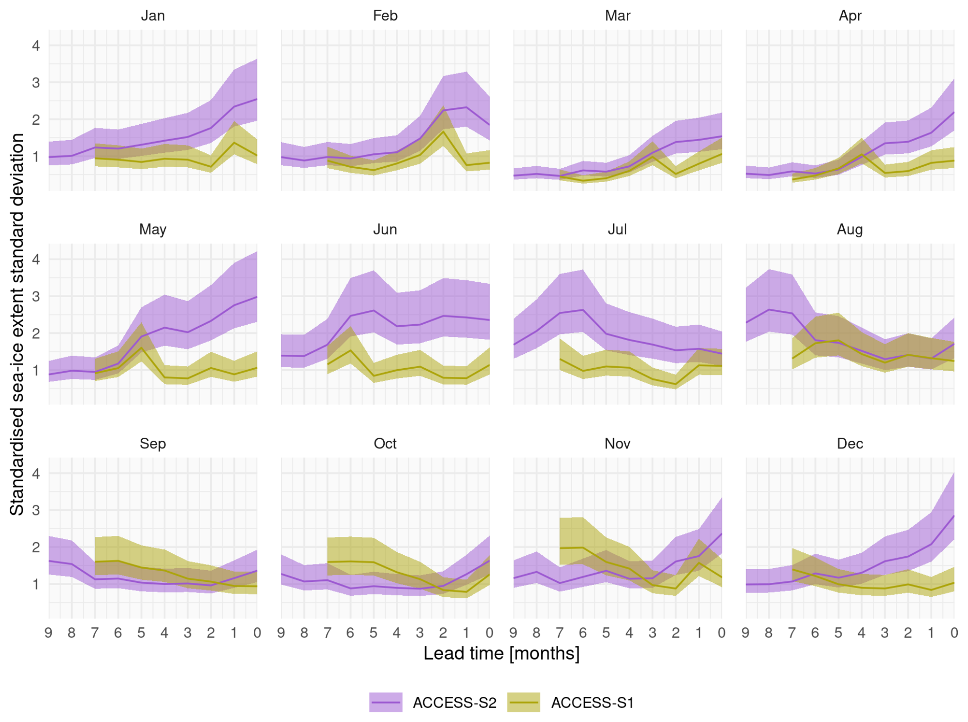
Figure A10 Interannual standard deviation with 95 % confidence interval of monthly mean sea-ice extent forecasted for each month. We standardise the standard deviation by that month's sea-ice extent observation standard deviation. Each panel indicates the target month. Note the reverse horizontal axis.

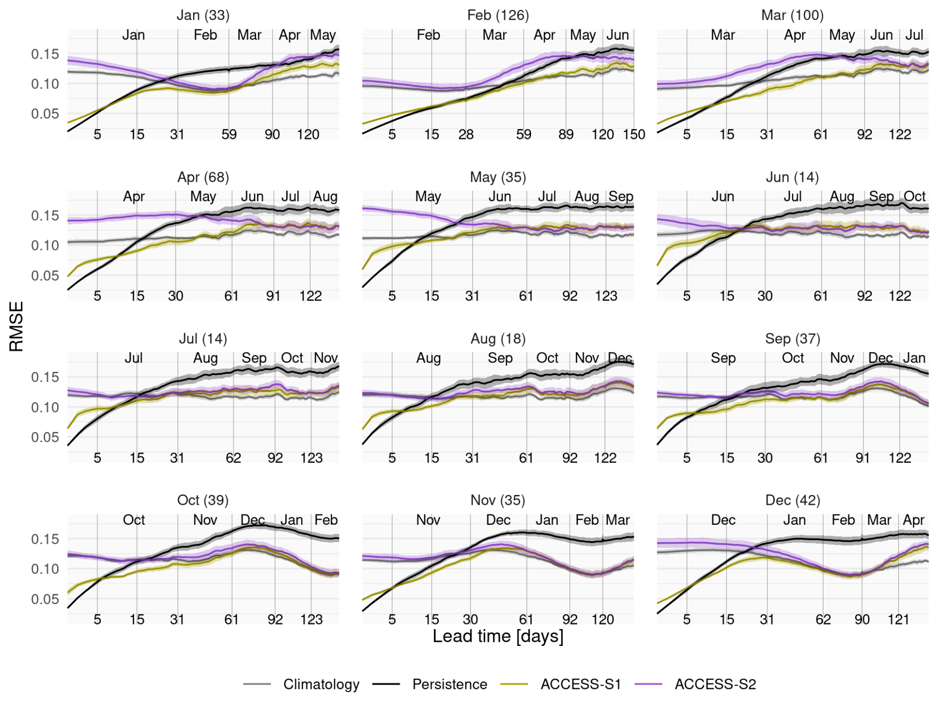
Figure A11 Mean RMSE of sea-ice concentration anomalies as a function of forecast lead time for all forecasts initialised on the first of each month compared with a reference forecast of persistence of anomalies (black) and climatology (gray). The shading indicates the 95 % confidence interval of the mean. Only the first 150 d are shown. In parentheses, the shortest time at which ACCESS-S1 and ACCESS-S2 mean RMSE is not statistically different at the 99 % confidence level. Note that the horizontal axis uses a square root transformation to expand the shorter lead times.

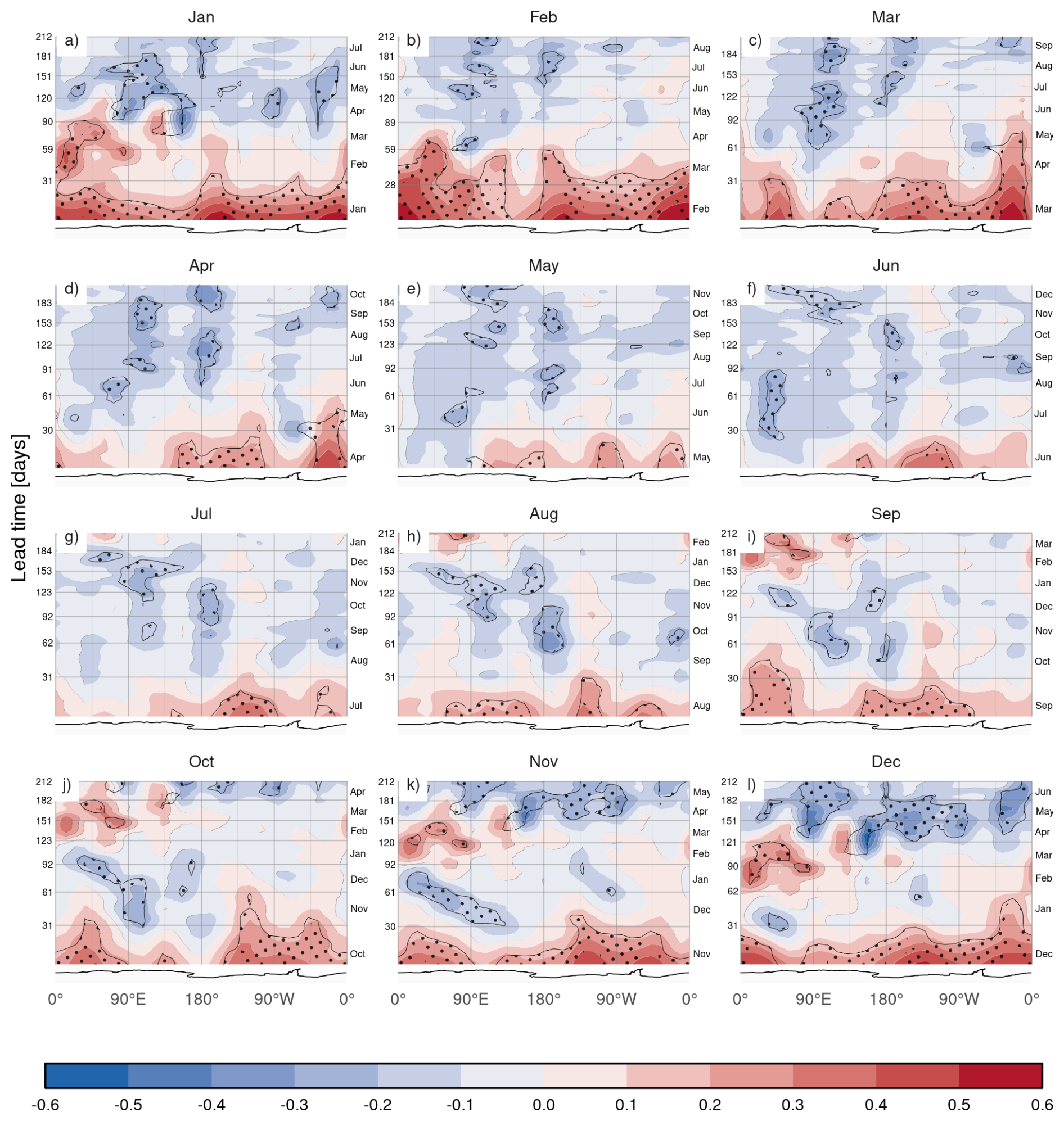
Figure A12 MSE skill score of ACCESS-S1 forecasts with climatological forecast as reference computed on 15 meridional slices 24° wide as a function of lead time and longitude. Regions where the difference of means between ACCESS-S1 RMSE and climatological RMSE are significant at p-value<0.05 are stipppled. Antarctica's coastline is shown at the bottom of each panel for reference. Values were smoothed with an 11 d running mean to improve readability. Note that the vertical axis uses a 1.5 root transformation to expand the shorter lead times.

Figure A13 Same as Fig. 11 but for ACCESS-S2.

Figure A14 Same as Fig. 11 but for the difference between ACCESS-S1 and ACCESS-S2.