the Creative Commons Attribution 4.0 License.
the Creative Commons Attribution 4.0 License.
 | 06 Nov 2020
Simultaneous estimation of wintertime sea ice thickness and snow depth from space-borne freeboard measurements
Hoyeon Shi
Byung-Ju Sohn
Gorm Dybkjær
Rasmus Tage Tonboe
Sang-Moo Lee
A method of simultaneously estimating snow depth and sea ice thickness using satellite-based freeboard measurements over the Arctic Ocean during winter was proposed. The ratio of snow depth to ice thickness (referred to as α) was defined and used in constraining the conversion from the freeboard to ice thickness in satellite altimetry without prior knowledge of snow depth. Then α was empirically determined using the ratio of temperature difference of the snow layer to the difference of the ice layer to allow the determination of α from satellite-derived snow surface temperature and snow–ice interface temperature. The proposed method was evaluated against NASA's Operation IceBridge measurements, and results indicated that the algorithm adequately retrieves snow depth and ice thickness simultaneously; retrieved ice thickness was found to be better than the methods relying on the use of snow depth climatology as input in terms of mean bias. The application of the proposed method to CryoSat-2 radar freeboard measurements yields similar results. In conclusion, the developed α-based method has the capacity to derive ice thickness and snow depth without relying on the snow depth information as input for the buoyancy equation or the radar penetration correction for converting freeboard to ice thickness.
- Article
(13610 KB) - Full-text XML
-
Supplement
(1204 KB) - BibTeX
- EndNote


Satellite altimeters have been used to estimate sea ice thickness for nearly 2 decades (Laxon et al., 2003, 2013; Kwok et al., 2009). The altimeters do not measure sea ice thickness directly but measure the sea ice freeboard which is then converted to sea ice thickness with assumptions, for example, regarding the snow depth, snow–ice densities, and radar penetration (Ricker et al., 2014). We hereafter refer to this procedure as “freeboard to thickness conversion”.
Generally, there are two types of satellite altimeters measuring different sea ice freeboards. (1) Lidar altimeters such as NASA's ICESat (Zwally et al., 2002) and ICESat-2 (Markus et al., 2017) missions measure the total freeboard (Ft), which is the height from the sea surface in leads to the snow surface. (2) Radar altimeters such as ESA's CryoSat-2 (CS2) (Wingham et al., 2006) measure the radar freeboard (Fr), which is the difference in the radar ranging between the sea surface and the radar scattering horizon. By applying two correction terms regarding the wave propagation speed change in the snow layer (Fc) and displacement of the scattering horizon from the ice surface (Fp), the radar freeboard is converted to the ice freeboard (Fi), which is the height from the sea surface to the snow–ice interface (Fi). Several studies indicate that the radar scattering horizon is at or above the snow–ice interface depending on ice type and snow–ice conditions (Nandan et al., 2017; Armitage and Ridout, 2015; Willatt et al., 2011; Tonboe et al., 2010). However, the radar scattering horizon is often treated as the snow–ice interface (Kurtz et al., 2014; Kwok and Cunningham, 2015; Hendricks et al., 2016; Guerreiro et al., 2017, Tilling et al., 2018). The three different freeboards are indicated in Fig. 1.

Figure 1Schematic diagram of a typical snow–ice system during the winter. Snow depth (hs), ice thickness (Hi), total freeboard (Ft), radar freeboard (Fr), and ice freeboard (Fi) are indicated. Correction terms regarding the wave propagation speed change in the snow layer (Fc) and the displacement of the scattering horizon from the ice surface (Fp) are indicated by blue arrows. The red line denotes a typical temperature profile with air–snow interface temperature (Tas), snow–ice interface temperature (Tsi), and ice–water interface temperature (Tiw).
For both lidar and radar altimeters, snow depth (hs) is required as an input to constrain the freeboard to thickness conversion; thus, the conversion results are highly dependent on snow depth (Ricker et al., 2014; Zygmuntowska et al., 2014; Kern et al., 2015). The buoyancy equation used in the freeboard to thickness conversion describes the balance between buoyancy and the weight of snow and ice. For a given freeboard, snow–ice densities, and assumptions on radar penetration of the snow layer, sea ice thickness (Hi) is a function of hs. According to Zygmuntowska et al. (2014), up to 70 % of uncertainty in the freeboard to thickness conversion stems from the poorly constrained snow depth. However, mapping the Arctic-scale snow depth distribution is challenging. The most commonly used snow depth information necessary for the freeboard to thickness conversion is the modified version of the snow depth climatology by Warren et al. (1999) (hereafter W99). W99 is based on in situ measurements from Soviet drifting stations (1954–1991) mostly of multiyear ice (MYI). Kurtz and Farrell (2011) compared W99 with Operation IceBridge (OIB) snow depth measurements in 2009 and claimed that W99 was still valid in the MYI region and significantly different from OIB snow depth on first-year ice (FYI). Based on that study, modified W99 (hereafter MW99) was developed, which halves W99 snow depth in regions covered by FYI. MW99 is often used in ESA's CryoSat-2 (CS2) ice thickness products available from the Center for Polar Observation and Modeling Data Portal (CPOM-UCL; Laxon et al., 2013), the Alfred Wegener Institute (AWI; Ricker et al., 2014), and the National Snow and Ice Data Center (NSIDC; Kurtz and Harbeck, 2017).
However, the use of MW99 for the freeboard to thickness conversion understandably yields a substantial error, considering that W99 is climatology and not actual snow depth. This is because the actual snow depth distribution is subject to the year-to-year variation of the snow–ice system; thus, the climatology based on the 37-year measurements of snow depth would deviate significantly from the actual distribution (Webster et al., 2014). Accordingly, such deviation causes errors in the estimation of ice thickness. Thus, additional snow observations covering both MYI and FYI at the Arctic basin scale would be ideal as a replacement of MW99.
There have been various approaches aimed at obtaining the snow depth distribution over the Arctic scale using satellite observations. Markus and Cavalieri (1998) developed an algorithm based on the brightness temperatures (TBs) of the Special Sensor Microwave/Imager (SSM/I) based on the negative correlation of the snow depth with the spectral gradient ratio between 18 and 37 GHz of vertically polarized TBs on the Antarctic FYI. Comiso et al. (2003) have updated the coefficients of this algorithm for the Advanced Microwave Scanning Radiometer for the Earth Observing System (AMSR-E). However, snow depth retrieval using this algorithm is relatively less accurate when the MYI fraction within the grid cell is significant (Brucker and Markus, 2013). Recently, Rostosky et al. (2018) suggested a new method: using the lower frequency pair of 7 and 19 GHz to overcome this limitation. Nonetheless, estimating the basin-scale snow depth distribution seems to be a difficult task.
There are other approaches involving the use of the lower frequency measurements at L-band. Using Soil Moisture Ocean Salinity (SMOS) measurements, Maaß et al. (2013) found that 1.4 GHz TB depends on the snow depth through the insulation effect of the snow layer, and they determined snow depth by matching TBs simulated with a radiative transfer model (RTM) with SMOS-measured TBs. Zhou et al. (2018) simultaneously estimated the sea ice thickness and snow depth by adding additional laser altimeter freeboard information, improving the Maaß et al. (2013) approach. However, both of these RTM-based approaches require a priori information on ice properties (e.g., temperature and salinity profiles).
Other satellite remote sensing approaches include the snow depth retrieval using dual-frequency altimetry (Guerreiro et al., 2016; Lawrence et al., 2018; Kwok and Markus, 2018), multilinear regression (Kilic et al., 2019), and a neural network approach (Braakmann-Folgmann and Donlon, 2019). In spite of promising results, the dual frequency altimetry method is available only for regions where two altimeters overlap with each other, reducing a great deal of spatial coverage. On the other hand, the regression/neural network methods based on AMSR-2 TBs are prone to the overfitting problem, limiting their applications to other microwave sensors.
Here, let us switch our point of view to solving the buoyancy equation instead of retrieving snow depth directly. Remember that there are two unknowns (snow depth and ice thickness) in the buoyancy equation for given snow–ice densities, freeboard, and assumptions on radar penetration of the snow layer. The attempt so far has been to add one constraint (snow depth information) to the buoyancy equation for solving ice thickness. However, if a particular relationship between two unknowns is available, it can be used to constrain the equation yielding both ice thickness and snow depth simultaneously.
To identify such a relationship, this study examines the vertical thermal structure within the snow–ice layers observed by drifting buoys. The vertical thermal structure of a snow–ice system in winter is rather simple; the temperature profile of the snow–ice system can be assumed to be piecewise linear, as illustrated in Fig. 1. Therefore, the temperatures at three interfaces can represent the thermal state of the snow–ice system fairly well: they are (1) air–snow interface temperature (Tas), (2) snow–ice interface temperature (Tsi), and (3) ice–water interface temperature (Tiw). Tiw is assumed to be nearly constant at the freezing temperature of seawater (Maaß et al., 2013), implying that the two other interface temperatures (Tas and Tsi) are sufficient to describe the thermal structure of the system.
Based on this thermal structure, there is a constraint relating the snow depth and ice thickness. In identifying this constraint, conductive heat flux is assumed to be continuous through the snow–ice interface (Maykut and Untersteiner, 1971), implying that conductive heat fluxes within the snow and ice layers are the same under the steady state assumed in the given thermal structure. As the conductive heat flux is proportional to the bulk temperature difference of the layer divided by its thickness, it is possible to deduce the relationship between snow depth and ice thickness from the given thermal structure.
Once the relationship is obtained, then it is possible to apply it at the Arctic Ocean basin scale because the thermal structure can be resolved from satellites, as shown in the recently available basin-scale and long-term satellite-derived interface temperatures (Dybkjær et al., 2020; Lee et al., 2018). In determining the snow depth along with the ice thickness, instead of using the snow depth as an input to solve for the ice thickness, we intend to (1) examine the relationship between the vertical thermal structure of a snow–ice system (Tas and Tsi) and the thicknesses of the snow and ice layer (hs and Hi) using buoy measurements and (2) retrieve the sea ice thickness and the snow depth simultaneously by applying their relationship to the freeboard to thickness conversion as a constraint, thus replacing the snow depth information. The result may reduce uncertainty in the freeboard to ice thickness conversion by replacing the currently used snow depth climatology.
Here we provide the theoretical background of how the snow–ice thickness ratio (α=hs ∕ Hi) can be related to Tas and Tsi. Then, after empirically determining the relationship of α to Tas and Tsi from buoy-measured temperature profiles, α obtained from satellite observed Tas and Tsi is then used to constrain the conversion from freeboard to ice thickness over the Arctic Ocean during winter.
2.1 Theoretical background
We intend to find a relationship between snow depth and ice thickness in terms of the vertical thermal structure of the snow–ice system. Because the temperature gradients within the snow and ice layers are linked to both temperature and thickness, we focus on the temperature gradient. Owing to the physical reasoning that the conductive heat flux is continuous across the snow–ice interface (Maykut and Untersteiner, 1971), the following relationship is valid at the snow–ice interface:
In Eq. (1), the subscripts snow and ice denote their respective layers, while T, k, and z denote temperature, thermal conductivity, and depth, respectively. The snow–ice interface is defined as z=0. Assuming a piecewise linear temperature profile within the snow–ice layer, Eq. (1) can be rewritten as follows:
where subscripts as, si, and iw denote the air–snow, snow–ice, and ice–water interface, respectively, and Hi and hs denote the sea ice thickness and snow depth as in Fig. 1. Introducing a variable α, which is the snow–ice thickness ratio, Eq. (2) becomes the following:
Here, ΔT denotes the temperature difference between the top and bottom of each of the snow and ice layers (i.e., , ). As explained in detail in Sect. 2.3, α can be used to constrain the freeboard to thickness conversion. Thus, once α is known, both snow depth and ice thickness can be simultaneously estimated from altimeter-measured freeboard instead of using snow depth data for ice thickness retrieval.
2.2 Empirical determination of “α-prediction equation” from buoy measurements
To obtain α, the conductivity ratio (ksnow ∕ kice) should be known even if the temperature difference ratio (ΔTsnow ∕ ΔTice) is given. In this study, instead of using the conventional conductivity ratio found in the literature, it is empirically determined using buoy-measured α and ΔTsnow ∕ ΔTice. Thus, the interface should be defined and determined from buoy-measured temperature profiles, which show a piecewise linear temperature profile as shown in Fig. 1.
The buoy-measured temperature profiles at the vertical resolution of 10 cm are used in this study (Sect. 3.1). Although the instrument initially sets the zero-depth reference position to be approximately at the snow–ice interface, the reference position can deviate from the initial location if the ice deforms or if the snow refreezes after the temporary melt into snow ice. In addition, the interfaces (air–snow, snow–ice, and ice–water) may be located in between measurement levels in a 10 cm spacing. Therefore, an interface searching algorithm is developed to determine three interfaces (yas, ysi, yiw) and their respective temperatures (Tas, Tsi, Tiw) by extrapolating each piecewise linear temperature profile iteratively.
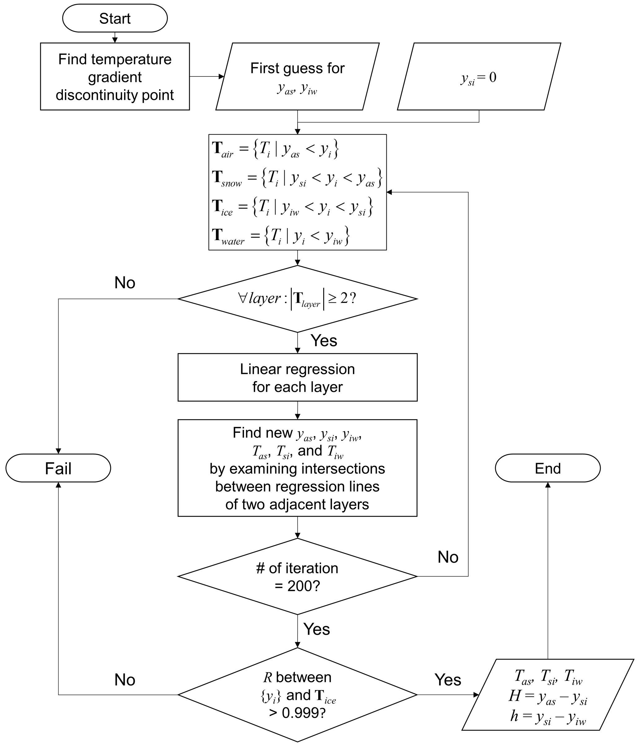
Figure 2The flow chart of the interface searching algorithm: yi and Ti denote the position and temperature of a data point in the temperature profile, yas,ysi, and yiw denote the position of the interfaces, and Tlayer denotes a set of temperature data points.
The interface searching algorithm iterates three processes to find the location and temperature of each interface: it (1) divides the temperature profile into four layers using the most recently available locations of the three interfaces, (2) finds a linear regression line of the temperature profile at each layer, and (3) updates the location and temperature of each interface by finding an intersection between two adjacent regression lines. The algorithm fails if the temperature profile is far from linear or if the thickness of a certain layer is too thin to have fewer than two data points. More detailed procedures for determining the interface are provided in Fig. 2 as a flow chart. The outputs are Tas, Tsi, Tiw, Hi (), and hs (). Examples of the interface searching results for 15 d averaged temperature profiles are shown in Fig. 3. The algorithm works adequately for both Cold Regions Research and Engineering Laboratory Ice Mass Balance (CRREL-IMB; Fig. 3a–c) and Surface Heat Energy Budget of the Arctic (SHEBA; Fig. 3d–f) buoy data.
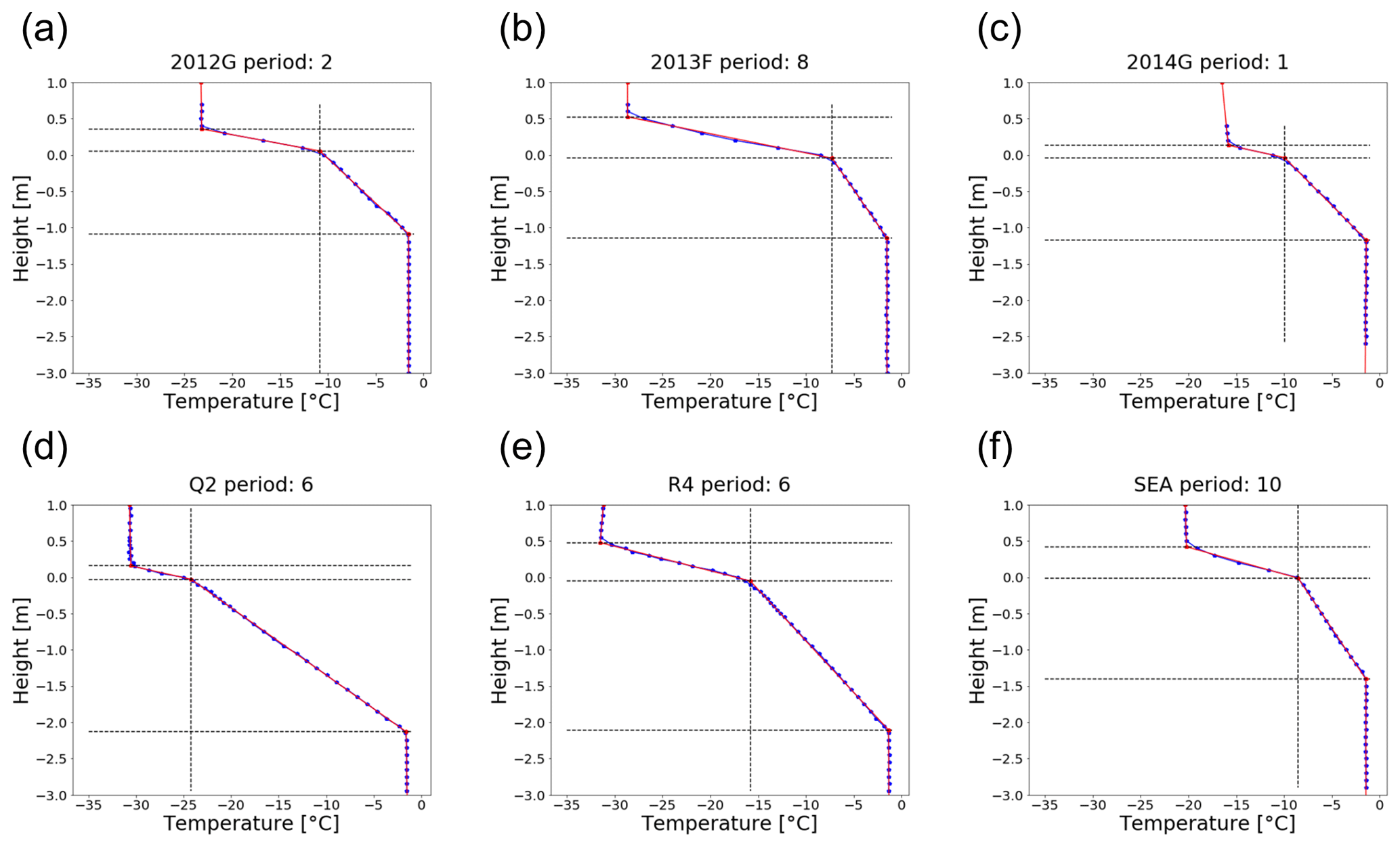
Figure 3Examples of interface searching results with an averaging period of 15 d: (a) 2012G period: 2, (b) 2013F period: 8, (c) 2014G period: 1, (d) Q2 period: 6, (e) R4 period: 6, and (f) SEA period: 10. The period number indicates the sequential 15 d period from 1 November (e.g., period: 2 denotes a time-averaging period of 16 to 30 November). Blue dots are buoy-measured temperature profiles, and red lines are regression lines. Dashed black lines indicate the intersections between adjacent regression lines.
Since Tas, Tsi, Tiw, Hi, and hs can be obtained from the previous interface determination with buoy data, the calculation of ΔTsnow ∕ ΔTice and α is straightforward. An empirical relationship can then be obtained by relating α to ΔTsnow ∕ ΔTice by running a regression model, and details are given in Sect. 4. However, for the time being, we assume that the regression equation (referred to as an “α-prediction equation”, which will be discussed in Sect. 4) is used to predict α from ΔTsnow/ΔTice.
2.3 Simultaneous estimation of ice thickness and snow depth from satellite-based freeboard using α
In this section, we describe how α can be used to constrain the freeboard to thickness conversion. Based on the assumed hydrostatic balance, ice thickness can be obtained from satellite-borne total freeboard or ice freeboard as follows:
Here, ρw, ρi, and ρs denote the bulk densities of the water, ice, and snow layers, respectively. Ice freeboard is obtained from radar freeboard by applying two correction terms regarding the change in the wave propagation speed in snow layer (Fc) and the displacement of the scattering horizon from the ice surface (Fp) (Kwok and Cunningham, 2015):
The correction terms are expressed in the following equations (Armitage and Ridout, 2015; Kwok and Markus, 2018):
Here, ηs denotes the refractive index of the snow layer and f denotes the radar penetration factor (Armitage and Ridout, 2015), which is the depth of the radar scattering horizon relative to the snow depth (e.g., f=1 if the radar scattering horizon is at the snow–ice interface and f=0 if the radar scattering horizon is at the air–snow interface). A combination of Eqs. (6)–(8) yields the following relationship:
Ice freeboard in Eq. (5) can be substituted by radar freeboard and snow depth using Eq. (9), i.e.,
According to Eq. (10), the ice thickness can be estimated from the radar freeboard and the snow depth. Note that Eq. (10) becomes equivalent to the equation for the total freeboard (Eq. 4 if f=0, i.e., if there is no radar penetration into the snow layer). With the use of α, defined in Eq. (3), Eqs. (4) and (10) become the following:
From Eqs. (3), (11), and (12), it is evident that the snow depth and ice thickness can be simultaneously estimated from the freeboards once α, ρ, f, and ηs are known.
In order to obtain α from satellite measurements of Tas and Tsi, we need to calculate the temperature difference ratio (ΔTsnow ∕ ΔTice). For the calculation, Tiw is set to be −1.5 ∘C. The freezing temperature of seawater is often assumed to be −1.8 ∘C; however, the value of −1.5 ∘C has been chosen based on the buoy observations. A sensitivity test indicated that the influence of a 0.3 ∘C difference in the freezing temperature on α was negligible (e.g., approximately 1.2 % difference for typical interface temperatures of ∘C and ∘C). The α values are calculated only at the pixel whose monthly sea ice concentration (SIC) is greater than 95 % and rejected if Tas is warmer than Tsi. The densities are prescribed with those used for OIB data processing: ρs, ρi, and ρw are 0.320, 0.915, and 1.024 g cm−3, respectively (Kurtz et al., 2013). Although ρs varies seasonally (Warren et al., 1999) and ρi is greater for MYI than FYI (Alexandrov et al., 2010), we use the same densities as those of OIB data because we intend to compare outputs against OIB data. In solving Eq. (12), cases showing negative ice thickness ( for the given densities and radar penetration factor) are rejected. Radar penetration factor f is set to be 0.84 for CS2 (Armitage and Ridout, 2015), and ηs is parameterized as a function of the snow density, i.e., (Ulaby et al., 1986).
Before the Arctic-basin-scale retrieval, ice thickness is estimated from OIB total freeboard measurements using Eq. (11) and from OIB-derived radar freeboards (Sect. 3.3) using Eq. (12) and using satellite-derived α as a constraint. At the same time, the corresponding snow depth is derived by multiplying the obtained sea ice thickness and α (Eq. 3). Sea ice thicknesses are also calculated from Eqs. (4) and (10) using MW99 as the snow depth to examine how simultaneous retrievals compare with ice thickness estimation using MW99. To differentiate various outputs, obtained snow depth and ice thickness are expressed with nomenclature such as (constraint, freeboard source). For example, the snow depth estimated from satellite-derived α and OIB total freeboard is referred to as hs (αsat, ), and sea ice thickness from the MW99 and OIB radar freeboard is referred to as Hi (, ). Finally, ice thickness and snow depth are estimated from CS2 radar freeboard (Sect. 3.4) over the Arctic Ocean.
Here we provide detailed information on the datasets used for the development of the retrieval algorithm, evaluation, and application at the Arctic Ocean basin scale.
3.1 CRREL and SHEBA buoy data
To determine the empirical relationship between α and ΔTsnow ∕ ΔTice using Eq. (3), we need information regarding hs, Hi, Tas, Tsi, and Tiw (as depicted in Fig. 1). These are sourced from temperature profiles observed by buoys deployed over the Arctic as part of the Surface Heat Energy Budget of the Arctic (SHEBA) campaign (Perovich et al., 2007) and the Cold Regions Research and Engineering Laboratory Ice Mass Balance (CRREL-IMB) buoy program (Perovich et al., 2019). Those buoy observations are stored for further analysis if there are no missing records over the entire period ranging from November to March of the following year. Detailed information regarding ice type and initial snow–ice thickness at deployment locations is given in Table 1.
Table 1Information on the measurement sites of buoys whose observations were used in this study.
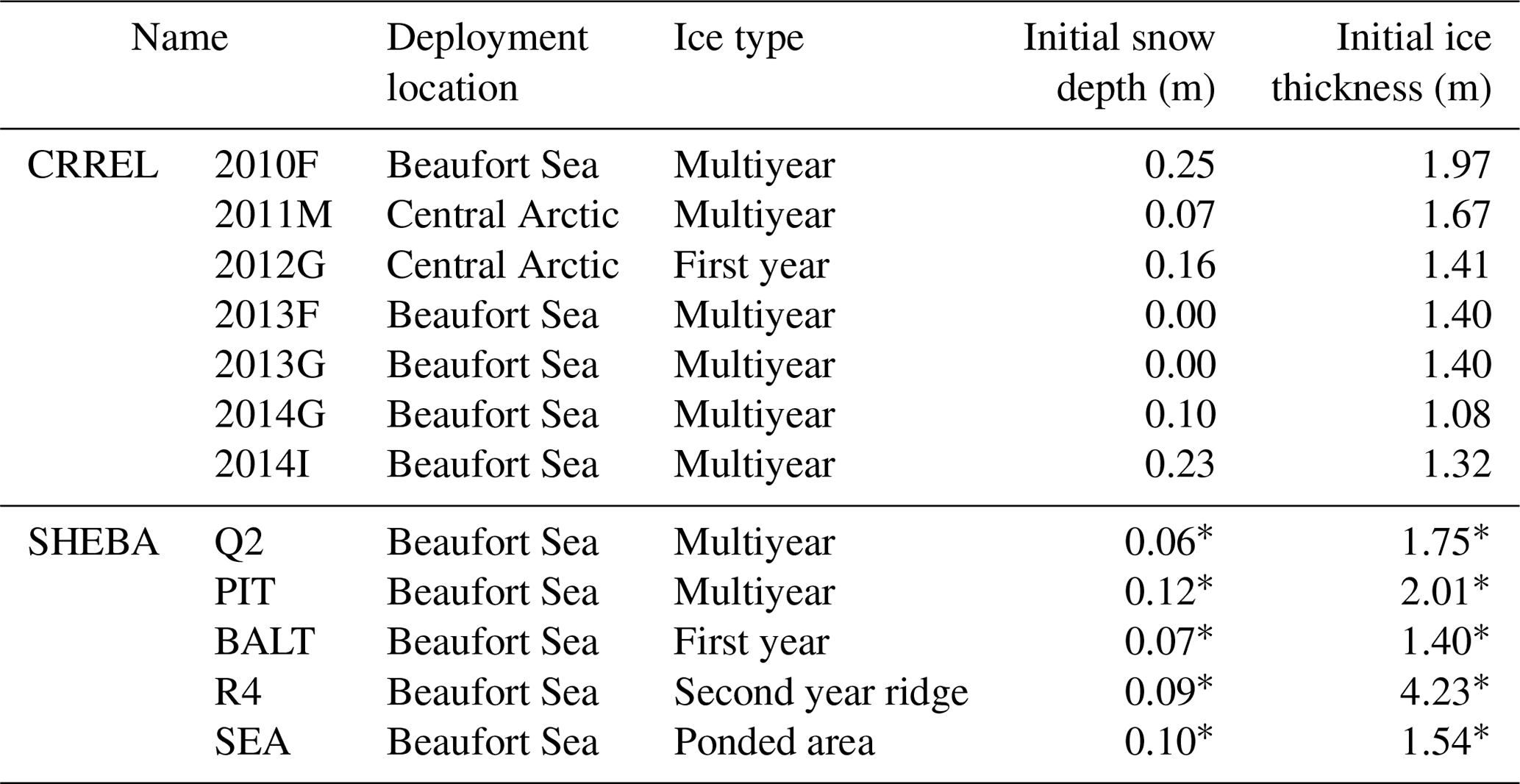
∗ The initial snow depth and ice thickness at the SHEBA sites are average values of all thickness gauge measurements in the corresponding site because there was one thermistor string but several thickness gauges at each measurement site.
Time averages of temperature profiles are used as input for the interface searching algorithm (described in Sect. 2.2) to meet the required near-equilibrium states (e.g., linear temperature profile). However, because of the possibility that the results are dependent on the averaging period, we examine the results using various averaging periods from 1 to 30 d.
3.2 Satellite-derived skin and interface temperatures
For applying the buoy-based α-prediction equation in retrieving the snow–ice thicknesses over the Arctic Ocean, satellite-derived Tas and Tsi data are necessary. In this study, Tas is obtained from the Arctic and Antarctic ice Surface Temperatures from thermal Infrared satellite sensors version 2 (AASTI-v2) data (Dybkjær et al., 2020), and the monthly mean for the 1982–2015 period is obtained from daily products. AASTI-v2 Tas is derived from the CM SAF cLouds, Albedo and surface RAdiation dataset from AVHRR (Advanced Very High Resolution Radiometer) data edition 2 (CLARA-A2) dataset (Karlsson et al., 2017), which is based on the algorithm described in Dybkjær et al. (2018). Information on the validation of this product is found in Dybkjær and Eastwood (2016). It is available in a 0.25∘ grid format; however, because other satellite datasets such as SIC are available in a 25 km Polar Stereographic SSM/I grid, AASTI-v2 data are re-gridded in the same 25 km grid format. This reformatted AASTI-v2 dataset is called “satellite skin temperature”.
Tsi is obtained from snow–ice interface temperature (SIIT) produced by Lee et al. (2018) over 30 years (1988–2017) of winters (December to February) using SSM/I and the Special Sensor Microwave Imager/Sounder (SSMIS) homogenized TBs (Berg et al., 2018). The daily data are in the 25 km grid format. Lee et al. (2018) reported that the satellite-derived Tsi is consistent with snow–ice interface temperatures observed by CRREL-IMB buoys, with a correlation coefficient, bias, and RMSE of 0.95, 0.15, and 1.48 K, respectively. In this study, we also produced Tsi for March using the same algorithm as Lee et al. (2018) for evaluating results against OIB data, which are mostly collected during spring. Monthly composites are constructed by averaging daily data for grid cells where the data frequency is over 20 d. This product is called “satellite interface temperature”.
3.3 OIB data
In this study, OIB snow depth () and total freeboard () are used as a reference in the evaluation of snow depth and ice thickness retrieved from the developed algorithm. NASA's OIB is an aircraft mission, and it measures snow depth and total freeboard over the Arctic using snow radar, Digital Mapping System (DMS), and Airborne Topographic Mapper (ATM) (Kurtz et al., 2013). OIB ice thickness is derived from measured snow depth and total freeboard for the given snow and ice densities using Eq. (4). In this study, the OIB radar freeboard () is derived from and using the combined relationship of and Eq. (9) as follows:
Because the main objective of using OIB data is to evaluate the relative performance of the simultaneous retrieval method when the method is applied to CS2 data, the radar penetration factor (f) for OIB data processing is also set to be 0.84. In the data processing chain, is removed if it is smaller than the given uncertainty level of the dataset (∼5.7 cm) or it is larger than the total freeboard .
The 5 years of OIB data during the 2011–2015 period are utilized in this study. The level 4 dataset (Kurtz et al., 2015) during the 2011–2013 period and Quick Look dataset during the 2014–2015 period are obtained from the NSIDC website (see the Data Availability section). Because we use the November–March period for the buoy analysis, only March OIB data are considered for the evaluation. The OIB data are also reformatted into the 25 km grid format by averaging pixel-level OIB observations on the 25 km grid.
3.4 CS2 data
For examining the Arctic Ocean basin distribution of ice thickness and snow depth, CS2 freeboard measurement summary data are used (Kurtz and Harbeck, 2017). They are monthly mean composites of CS2 ice freeboard data in the 25 km Polar Stereographic SSM/I grid format covering the entire Arctic and available from September 2010. Detailed descriptions of the retracker algorithm used in this dataset are found in the study by Kurtz et al. (2014). The dataset also includes MW99 () and W99 snow density climatology used for producing the ice freeboard.
The CS2 ice freeboard data () distributed by NSIDC (Kurtz and Harbeck, 2017) assumed that the radar scattering horizon is at the snow–ice interface and applied a wave propagation speed correction. However, the correction was made using and W99 snow density climatology with an erroneous form of ) hs instead of the proper form of ) hs (Mallett et al., 2020). Thus, at this point, it is straightforward to derive the CS2 radar freeboard by removing the correction term, as in the following equation:
Here, ηs was parameterized as a function of the snow density, i.e., (Tiuri et al., 1984), and ρs is taken from the W99 climatology based on Kurtz and Harbeck (2017). Then CS2 ice thickness is reproduced from and by using Eq. (10) with the constant densities and the radar penetration factor described in Sect. 2.3. Those and , ) values are used for comparison with results from our simultaneous method.
3.5 Sea ice concentration
Calculation of α is done for those pixels whose monthly SIC is greater than 95 % (as described in Sect. 2.3). To determine pixels that meet this SIC criterion, “bootstrap sea ice concentrations from Nimbus-7 SMMR [Scanning Multichannel Microwave Radiometer] and DMSP [Defense Meteorological Satellite Program] SSM/I-SSMIS version 3” produced by Comiso (2017) are used. This SIC dataset is provided in the 25 km Polar Stereographic SSM/I grid format.
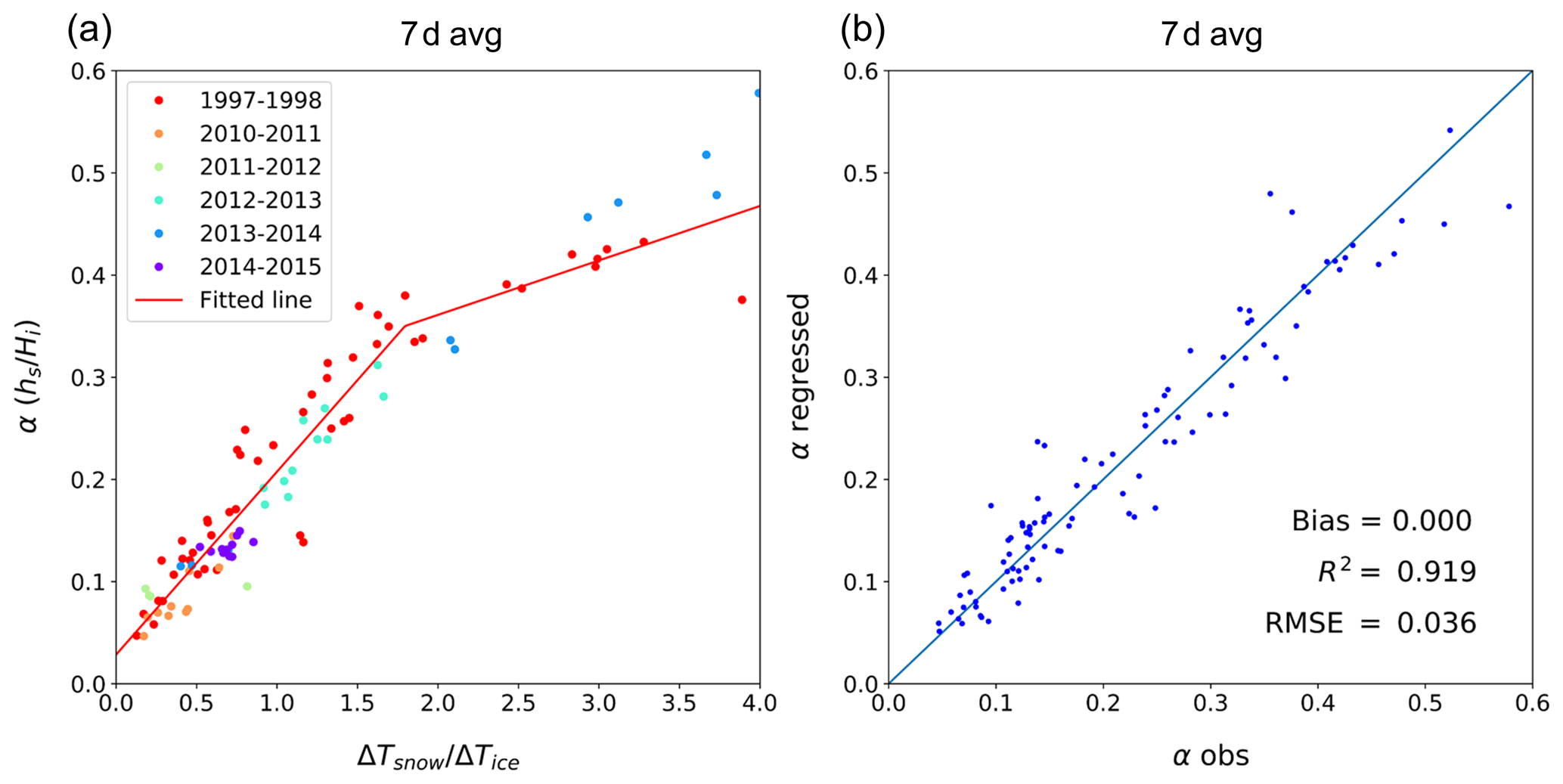
Figure 4(a) Scatterplots of the temperature difference ratio of the snow and ice layer (ΔTsnow ∕ ΔTice) and the snow–ice thickness ratio (α). Color denotes the collected year of buoy data. The red lines are the regression lines (defined in Eq. 15). (b) The scatter plot of observed and regressed α.
4.1 The empirical relationship between α and ΔTsnow ∕ ΔTice
We examine variables (i.e., Tas, Tsi, Tiw, Hi, and hs) obtained from buoy observations by applying the interface searching algorithm. In the scatter plot of weekly averaged ΔTsnow ∕ ΔTice vs. α (Fig. 4a), it appears that α linearly increases with ΔTsnow ∕ ΔTice when the ratio is smaller than 1.8, but the linear slope becomes smaller when ΔTsnow ∕ ΔTice is larger than 1.8. This pattern of the slopes is found to be nearly invariant from year to year, as is observed in the different colors appearing in the entire range of ΔTsnow ∕ ΔTice in Fig. 4a. We also found that this slope pattern is of a consistent nature even for different datasets; two different datasets (red points for SHEBA and other points for CRREL) covering various ranges of ΔTsnow ∕ ΔTice show similar distributions along the two different slopes. Thus, the slope pattern is not due to different data sources or different data periods. Further analysis of the two slopes is found in Appendix A.
Taking such a two-slope pattern with ΔTsnow ∕ ΔTice into account, we introduce a piecewise linear function that may express the slope pattern, i.e.,
In Eq. (15), x and y correspond to ΔTsnow ∕ ΔTice and α, respectively, and x0 is the point where the slope transition takes place. Applying Eq. (15) to data points from buoy-based variables, the regression coefficients (a1, b1, a2, b2) and transition point (x0) are determined by minimizing the total variance – the obtained regression line is plotted in Fig. 4a. The α value is predicted using the determined regression equation (hereafter referred to as the α-prediction equation) and compared to the original α values to see how well the regression was performed. The comparison of α with predicted values in Fig. 4b shows that the regression equation is well fitted because of the zero bias and 91.9 % of explained variance.

Figure 5(a) The regression coefficients (a1, b1, a2, b2) in Eq. (15) and (b) the error statistics of the regression with averaging periods from 1 to 30 d.
Table 2Coefficients of the regression equation for averaging periods of 1, 7, 15, and 30 d; a1, b1, a2, b2, and x0 are given in Eq. (15).
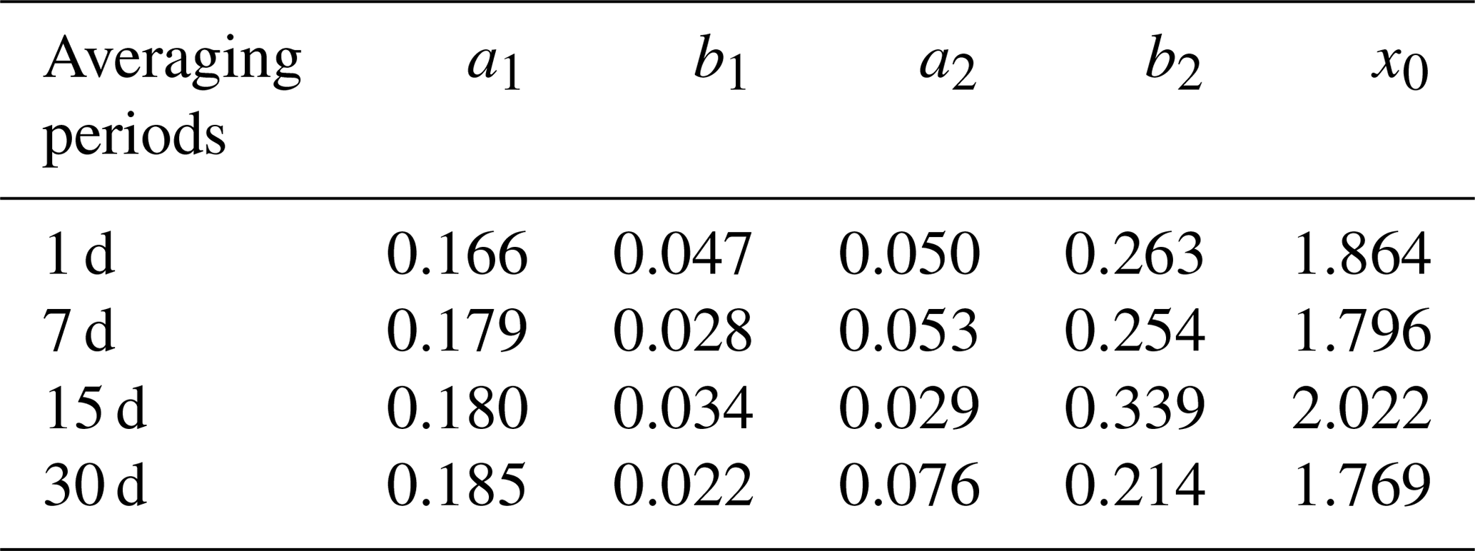
Although the slope pattern discussed with Eq. (15) and Fig. 4 is based on the weekly averages, the slope pattern seems to be consistent among the data averaging periods except for an averaging period shorter than 5 d. Regressions in the form of Eq. (15) are performed with buoy data averaged with different averaging periods to understand the slope pattern. The regression coefficients and transition points for the chosen averaging periods are examined, and results for four averaging periods are given in Table 2. Detailed information on the coefficients and associated statistics varying with the averaging period is given in Fig. 5. The positions of slope change (x0) are located at approximately 1.8, delineating a nearly invariant slope pattern regardless of different data averaging periods. Figure 5a shows that coefficients do not vary much with different averaging periods, while coefficients of the first part of the regression line (a1 and b1, x≤x0) vary less than those of the second part (a2 and b2, x>x0). The regression equations show that the explained variance (R2) rises quickly when the averaging period is longer but levels off when data are averaged over a period that is longer than 7 d. The bias appears to be near zero over the various averaging periods. Thus, the regression performance is found to be comparable if data are averaged over a period that is longer than 1 week.
4.2 Evaluation against OIB estimates
According to the regression results, it is possible to estimate α from ΔTsnow ∕ ΔTice. Since ΔTsnow ∕ ΔTice can be calculated from the satellite skin and interface temperature (as described in Sect. 3.2), the corresponding α can be estimated from satellite measurements. Thus, we are able to simultaneously retrieve sea ice thickness and snow depth from altimeter-based freeboard measurements following Eqs. (11) and (12). We test and evaluate this simultaneous retrieval approach using OIB data. Accordingly, ice thickness and snow depth are simultaneously estimated from OIB freeboard measurements and evaluated against the OIB snow depth () and ice thickness ().
To calculate α, a data averaging period must be selected. Considering that the monthly composite of satellite freeboard measurements is needed to retrieve snow–ice thickness at the Arctic basin scale, it seems appropriate to use the monthly averaging period to calculate the monthly α distribution. Thus, we use the monthly averaged satellite temperatures and the coefficients for the 30 d averaging period (Table 2) to calculate α.
We simultaneously retrieved Hi and hs for March of each year during the 2011–2015 period from the reformatted OIB freeboard measurements (Sect. 3.3), together with satellite-derived α (αsat). As expressed in Eqs. (11) and (12), two different ice thickness retrievals are possible depending on the use of the freeboard type (i.e., total freeboard Ft vs. radar freeboard Fr). Two accordingly associated retrievals of snow depth are available. Retrieved results of ice thickness (Hi) and snow depth (hs) from the use of OIB total freeboard and radar freeboard are given in the first and second row of Fig. 6, respectively. Corresponding OIB measurements are given at the bottom of Fig. 6. The comparison between any snow–ice retrievals and OIB measurements appear to be consistent with each other for both snow depth and ice thickness in terms of magnitudes and distribution.
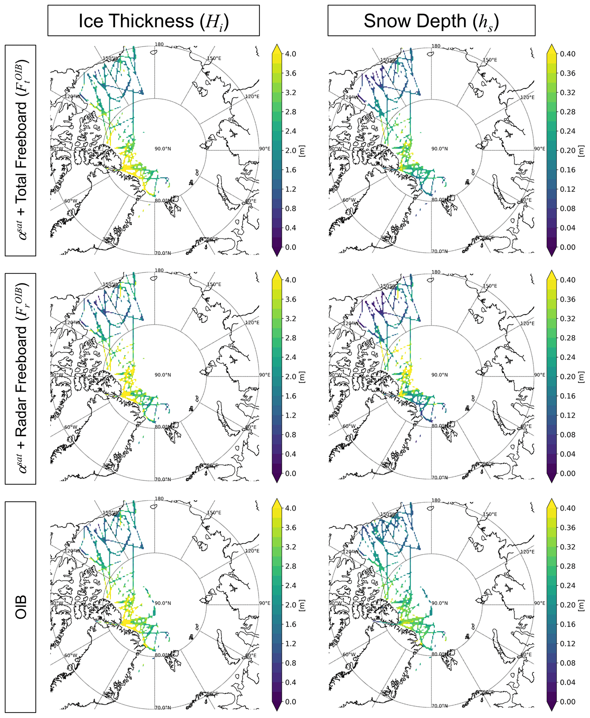
Figure 6Simultaneously retrieved ice thickness and snow depth from OIB total and radar freeboards in March of the 2011–2015 period. Corresponding OIB products are at the bottom.
To compare the results quantitatively, scatterplots comparing retrievals against OIB measurements are made, along with statistics for the snow depth and ice thickness retrievals, in the top four panels of Fig. 7. The two top-left panels are derived from the use of OIB total freeboard (), while the two top-right panels are derived from the OIB radar freeboard (). The comparison is done only for pixels for which all four products (i.e., snow–ice thicknesses from two different freeboards) are available. This indicates that the snow depth from the total freeboard (top left) is fairly consistent with the OIB snow depth with a correlation coefficient of 0.73 and with a near-zero bias. The retrieved ice thickness from the total freeboard (middle left) appears to be consistent with OIB ice thickness with a correlation coefficient of 0.93 and a bias around 8.5 cm. The RMSEs for snow depth and ice thickness are 6.8 cm and 44.3 cm, respectively. Based on the comparison results, Eq. (15) obtained from buoy measurements can be successfully implemented with space-borne total freeboard measurements for the simultaneous retrieval of snow depth and ice thickness.
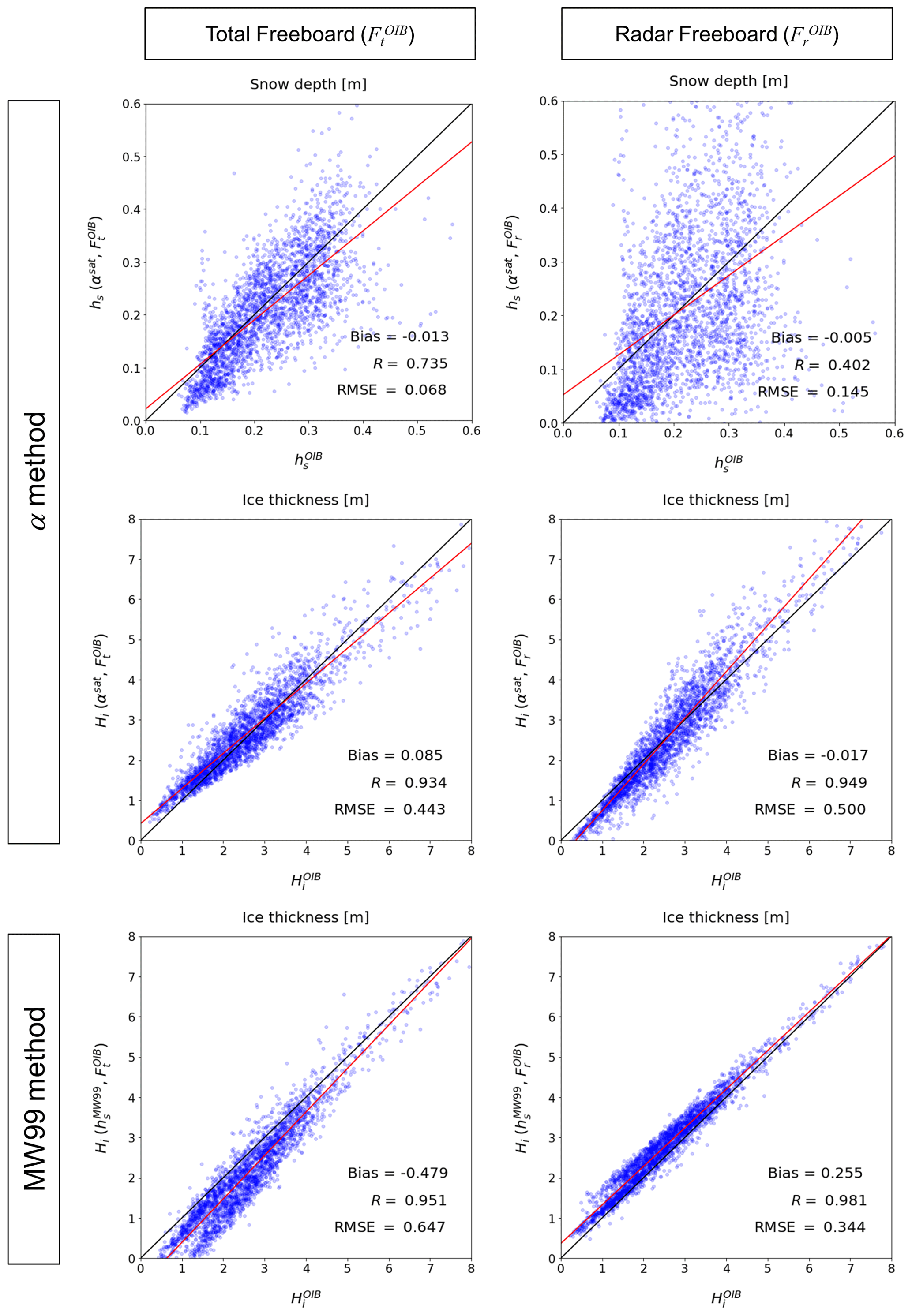
Figure 7Scatter plots between OIB products and the simultaneously retrieved snow depth and ice thickness from OIB total and radar freeboards during the March 2011–2015 period. Corresponding ice thicknesses estimated from MW99 are in the third row. The red lines are linear regression lines.
Following Eq. (12), snow depth and ice thickness retrievals are made from the use of radar freeboard measurements, and results are presented in the two top-right panels in Fig. 7. On the one hand, the comparison of obtained ice thickness against the OIB ice thickness indicates that the retrieved ice thickness shows a similar quality as that retrieved from the total freeboard measurements. On the other hand, snow retrievals from the radar freeboard show more scattered features compared to snow retrieval results from the total freeboard. The more scattered features found in the snow depth from the radar freeboard are likely due to the greater sensitivity of the retrieved α and the prescribed densities, as noted in Eq. (12). Note that Eq. (12) has a smaller denominator than that of Eq. (11). Results of the associated sensitivity analysis can be found in Appendix B.
We now examine how the use of MW99 for retrieving sea ice thickness from ICESat and CS2 measurements compares with results from our simultaneous method. To do so, OIB-measured total freeboard and radar freeboard are converted into ice thickness using MW99 as the input to solve Eqs. (4) and (10). In this study, these two ice thickness retrievals with the use of MW99 are referred to as “ICESat-like” thickness and “CS2-like” thickness, respectively, and their comparisons are now observed in the two panels at the bottom of Fig. 7. According to our analysis, ICESat-like thickness tends to underestimate the ice thickness by about 47.9 cm when MW99 is used in comparison to OIB thickness, and CS2-like ice thickness shows an overestimate of about 25.5 cm. Nevertheless, their correlation coefficients and RMSEs are similar to the results obtained from the α method.
The better agreement of Hi from the simultaneous method with may be due to the fact that the simultaneously estimated hs is more consistent with ( is likely larger than , as shown in Fig. S1). Note that all inputs are the same except the snow depth. The negative bias of ICESat-like thickness and positive bias of CS2-like thickness reflect expected responses in different signs to the same snow depth error, as shown in different signs in the last terms of Eqs. (4) and (10) (also note Eq. B2 in Appendix B). Because of this reasoning, if there are decreasing trends not only in ice thickness but also in snow depth, the decreasing trend of ice thickness estimated from the constant snow depth will be diminished in radar while being amplified in lidar. Because of this, the construction of the ice thickness (or volume) trend from the two different satellite altimeters would be problematic if MW99 is used for the freeboard to thickness conversion. For example, it would be hard to compare the sea ice thickness records estimated from ICESat and CS2 observations and to extend the current ice thickness record from CS2 with NASA's recently launched ICESat-2, which carries a lidar altimeter, for the same reason.
4.3 Simultaneous retrieval of ice thickness and snow depth from CS2 measurements
We have demonstrated that the method of simultaneously retrieving the sea ice thickness and snow depth was successfully implemented with OIB measurements. Now we extend the proposed approach to satellite freeboard measurements. Here the method is tested with CS2 freeboard measurements, solving for Hi in Eq. (12), and α is obtained from the collocated satellite skin and interface temperature data.
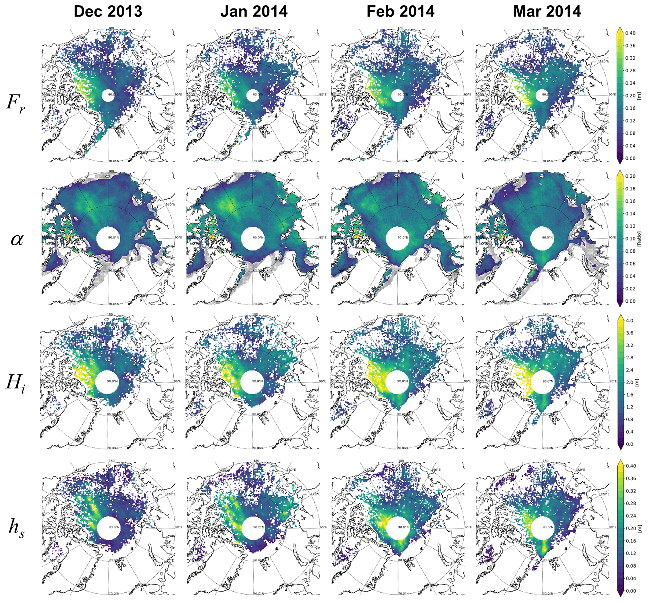
Figure 8Geographical distributions of observed CS2 radar freeboard (Fr) and estimated snow–ice thickness ratio (α), ice thickness (Hi), and snow depth (hs) from December 2013 to March 2014. Gray areas in the second row denote where α retrievals failed because Tas was warmer than Tsi.
Monthly means of CS2-estimated freeboard (Fr), retrieved α, ice thickness (Hi), and snow depth (hs) for December 2013 to March 2014 are given in Fig. 8. The geographical distribution of α indicates that α is largest in January and becomes smaller during the following months. Geographically, there seems to be no particular distribution of α between months, although interestingly the lowest α values are always found over the north of the Canadian Archipelago, and the western part of the Arctic Ocean shows α values that are generally larger than those over the eastern part.
Retrieved ice thickness from the CS2 freeboard (Fr) using obtained α is presented in the third row of Fig. 8. As expected and as noted in Eq. (12), Hi shows a similar geographical distribution to radar freeboard (the first row). The thickest area is located north of the Canadian Archipelago where the ice appears thicker than 4 m. On the other hand, most of the FYI thickness appears to range from 1.0 to 2.0 m. The snow depth hs is obtained by multiplying α by Hi (in 2nd and 3rd rows), following Eq. (3), and results are shown in the bottom row. The obtained snow distribution indicates that thicker (thinner) snow areas are generally coincident with thicker MYI (thinner FYI) areas. Such a similarity should be consistent with the notion that MYI should accumulate more precipitation than FYI because of its longer existence.
To assess the accuracy of CS2 retrievals, reference snow depth and ice thickness collocated with CS2 freeboard in space and time are necessary. However, different from simultaneous retrievals from OIB freeboards in Sect. 4.2, the evaluation with the required matching data may not be possible from the monthly composite of CS2 data used in this study. Here, instead of using monthly collocated match-up data, an indirect way is used to examine the accuracy of CS2 retrievals. We do so by examining whether the relationship between the simultaneous method and the MW99 method, based on retrievals from the OIB freeboard, can be reproduced by CS2-based retrievals. If similar results are obtained, respective accuracies can be deduced against those noted from the evaluation against OIB measurements.
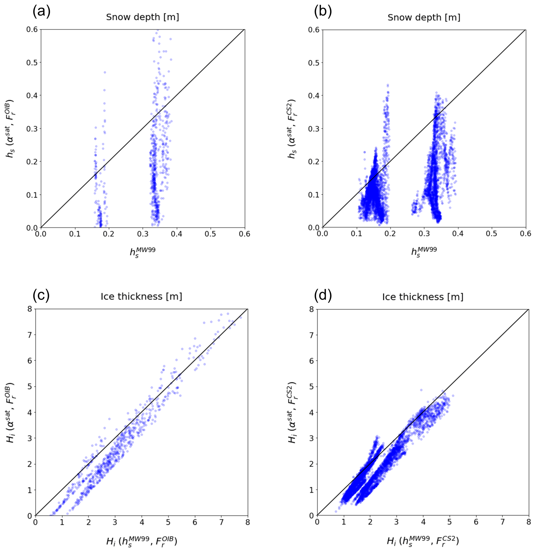
Figure 9Comparison of simultaneously retrieved snow depth and ice thickness to those from the MW99 method. (a) Snow depth from OIB radar freeboard, (b) snow depth from CS2 radar freeboard, (c) ice thickness from OIB radar freeboard, and (d) ice thickness from CS2 radar freeboard.
The relationships which can be obtained from the analysis in Sect. 4.2 – i.e., hs (αsat, ) vs. and Hi(αsat, ) vs. Hi (, ) – are compared with the relationships found in the current results in Fig. 8 – i.e., hs (αsat, ) vs. and Hi(αsat, ) vs. Hi (, ); the results are presented in Fig. 9. Observably, the relationships from CS2 freeboard data (Fig. 9b, d) are very similar to the relationship obtained from the comparison results from OIB measurements (Fig. 9a, c). This similarity of the slope strongly indicates that the CS2-based sea ice thickness from the current α method has similar accuracy to that found in the evaluation against OIB measurements (Sect. 4.2). Further uncertainty estimates for CS2-derived products can be found in Appendix C.
A new approach towards simultaneously estimating snow depth and ice thickness from space-borne freeboard measurements was proposed and tested using OIB data and CS2 freeboard measurements. In developing the algorithm, the vertical temperature slopes were assumed to be linear within the snow and ice layers so that a continuous heat flux could be maintained in both layers. This assumption allowed for the description of the snow–ice vertical thermal structure with snow skin temperature, snow–ice interface temperature, the water temperature at the ice–water interface, snow depth, and ice thickness. Based on the continuous heat transfer assumption, the snow–ice thickness ratio (α=hs ∕ Hi) was introduced and could then be embedded into the freeboard to ice thickness conversion equations. Thus, information on both ice thickness and snow depth can be derived once α is known in the case of the availability of a freeboard without relying on the snow depth information as an input for the conversion from freeboard to ice thickness. From the drifting buoy measurements of the temperature profile, snow depth, and ice thickness over the Arctic Ocean, we demonstrated that α can be reliably determined using the ratio of the vertical difference of the snow layer temperature to the vertical difference of ice layer temperature (ΔTsnow ∕ ΔTice). An empirical regression equation was obtained for predicting α from three interface temperatures.
Before applying the α-prediction equation to simultaneously retrieve the ice thickness and snow depth from satellite-borne freeboard measurements, the algorithm was evaluated using OIB measurements in conjunction with satellite-derived snow skin temperature and snow–ice interface temperature. The evaluation of results demonstrated that our proposed algorithm adequately retrieved both parameters simultaneously. As a matter of fact, the ice thickness results were more accurate than they were from the current retrieval methods relying on the input of snow depth (this time MW99 snow climatology) in terms of mean bias. It should be noted that in this case, snow depth is a retrieval product instead of being input for the freeboard to ice thickness conversion adopted by CS2 or ICESat retrieval. The application was finally made for the retrieval of the snow depth and ice thickness from CS2 radar freeboard measurements from December 2013 to March 2014 using α as a constraint. Results showed that the quality of the obtained ice thickness was similar to that obtained from evaluation results against OIB measurements. Retrieved snow depth distributions were also found to be consistent with expectations.
In the retrieval process, we may be concerned about the applicability of the algorithm developed with buoy observations representing the point measurements to the larger spatial and temporal scales of satellite measurements. This concern may be relevant upon observing the range of α values. The α value in the satellite's monthly and 25 km × 25 km spatial scales was found to be generally smaller than 0.2. The smaller range of α compared to that shown in the buoy analysis results is likely due to the scale differences, indicating that extreme α values often shown in buoy measurements (due to very thick snow and/or very thin ice) may never be observed in satellite measurements. However, the range may not be a problem because the relationship (Eq. 3) expresses the thermal equilibrium condition described by the temperature at three interfaces, the ratio of snow and ice thickness, and the ratio of thermal conductivity between snow and ice. Considering that the algorithm is based on the equilibrium conditions, results should be valid regardless of spatial and temporal scales if the prerequisite equilibrium conditions are met. Apparently, buoy observations contain so many different cases that equilibrium conditions are met with different thermal and physical conditions of the snow–ice system. The sound evaluation results and the consistency between OIB and CS2 ice thickness retrieval results, which are subject to different scales, all suggest that the point-measured α-prediction equation can apply to satellite measurements.
Overall, the developed α-based method yields ice thickness and snow depth without relying on a priori “uncertain” snow depth information (MW99), which results in uncertainty in the ice thickness retrieval. The proposed method applies to both lidar and radar altimeter data, although lidar-based altimeter data tend to offer relatively more suitable snow depth information with a smaller RMSE. We expect to continuously monitor the Arctic-scale snow depth and ice thickness by applying the proposed α method to total freeboard observations from the recently launched ICESat-2 and using temperature observations from the upcoming MetOp-SG meteorological imager (MetImage), the microwave imager (MWI), and the proposed Copernicus Imaging Microwave Radiometer (CIMR).
The relationship found between α and ΔTsnow ∕ ΔTice showed a piecewise linearity which is almost invariant to the data averaging period. Because the slope change is attributable neither to different data sources nor to different data periods, it is likely caused by the physical properties of the snow and ice, as shown in Fig. A1. If the slope change is caused by the snow–ice condition, there will be a significant difference in snow–ice properties between the two parts showing different slopes. Here we examine the possibility of different physical properties causing the difference in slopes. Through this comparison using buoy data, we may identify important properties that might be responsible for the piecewise linearity.
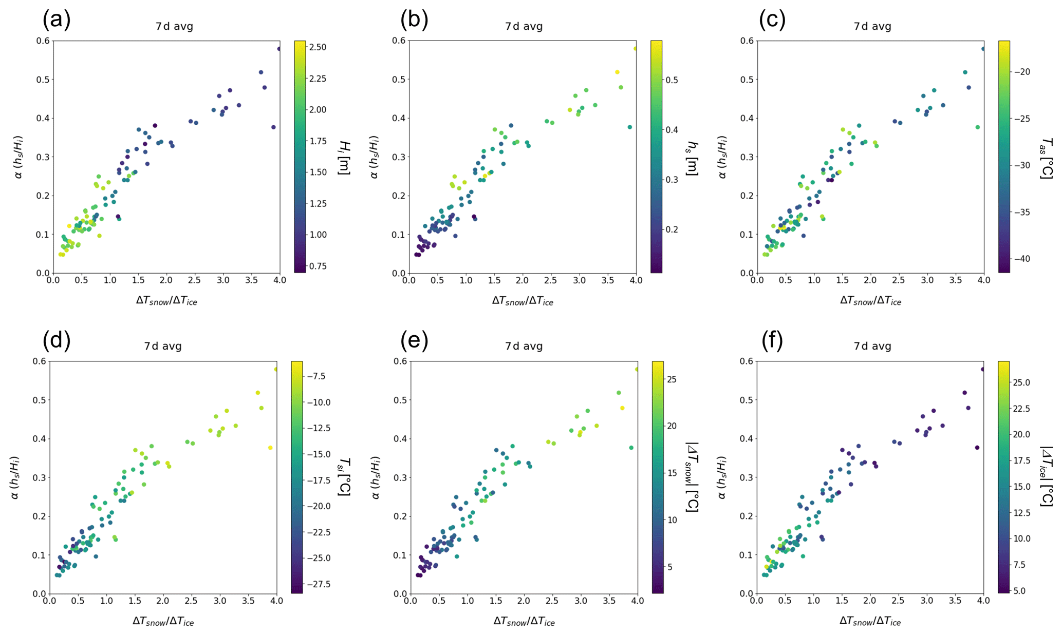
Figure A1Distribution of physical variables on scatterplots of the temperature difference ratio of snow and ice layer (ΔTsnow ∕ ΔTice) and the snow–ice thickness ratio (α). Color denotes the value of physical variables: (a) ice thickness (Hi), (b) snow depth (hs), (c) air–snow interface temperature (Tas), (d) snow–ice interface temperature (Tsi), (e) temperature difference within the snow layer (), and (f) temperature difference within the ice layer ().
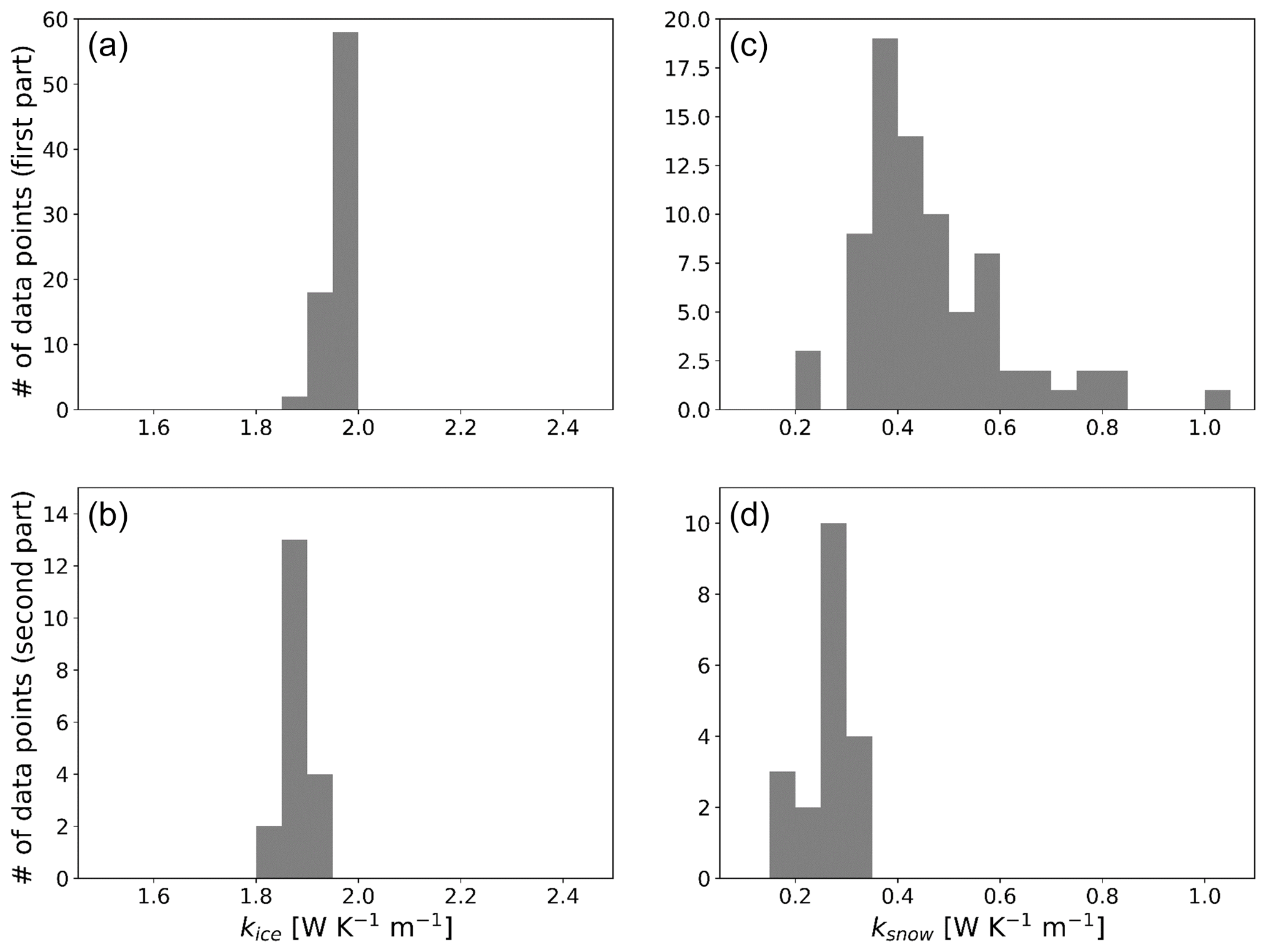
Figure A2Histogram of estimated (a, b) kice and (c, d) ksnow. The top and bottom rows denote the first and the second parts, respectively. The size of the bins is 0.05 W K−1 m−1.
First, the averages of basic properties available from buoy measurements are compared. They include ice thickness, snow depth, snow–ice interface temperature, ice temperature – – and so on. The comparison revealed that snow–ice system within the first part (x≤x0) is found to consist of relatively thicker ice (mean value: 1.84 m), thinner snow (0.29 m), and colder ice (−9.13 ∘C), while the second part (x >x0) is found to consist of relatively thinner ice (1.10 m), thicker snow (0.46 m), and warmer ice (−5.00 ∘C). In general, a thicker snow or ice layer exhibits a greater temperature difference from the top to the bottom of the layer. There is no significant difference between the air–snow interface temperature (Tas) in the two slope parts.
The thermal conductivities, ksnow and kice, are also compared because what connects α and ΔTsnow ∕ ΔTice is the ratio of thermal conductivities. Before showing the results, we describe how to calculate ksnow and kice. First, the thermal conductivity ratio is calculated from buoy-measured variables (i.e., Tas, Tsi, Tiw, hs, and Hi) using Eq. (3). Because the underlying physics in ksnow are significantly more complex, kice is estimated first, and then ksnow is obtained by multiplying the calculated kice by ksnow ∕ kice. To calculate kice, the parameterization of Maykut and Untersteiner (1971), which describes kice as a function of salinity and temperature, is used:
Here, Sice and Tice are the salinity (in parts per thousand, ppt) and temperature (in Celsius) of sea ice, respectively. For the calculation, Sice is estimated according to the empirical relationship between sea ice thickness and mean salinity from Cox and Weeks (1974) as follows:
Although Trodahl et al. (2001) reported that kice depends on depth and temperature, here we do not estimate accurate thermal conductivities but attempt to examine the physical consequences of the total ice layer.
The calculated thermal conductivities are presented in Fig. A2. The calculated kice ranges from 1.8 to 2.0 W K−1 m−1 (two left panels in Fig. A2). These values are consistent with the in situ measurements by Pringle et al. (2006). The mean values of kice of the first part (1.96 W K−1 m−1) and the second part (1.88 W K−1 m−1) show almost no difference. The calculated ksnow ranges from 0.2 to 1.05 W K−1 m−1 (two right panels in Fig. A2). This range is consistent with reported values in Sturm et al. (1997). The first part shows the greater spread in the distribution of ksnow compared to the second part. The mean ksnow values are 0.44 and 0.27 for the first part and second part, respectively.
As a significant difference is observed in ksnow, we would like to find a possible reason for this difference. To do so, we should first review the factors determining ksnow; they are density, temperature, and crystal structure (Sturm et al., 1997). Snow is a mixture of ice particles and air, and air has lower thermal conductivity than ice. Thus, snow with a relatively lower density including a greater portion of air should have relatively lower thermal conductivity. Besides, the thermal conductivity of ice particles depends on the temperature, and the path of heat transfer depends on the crystal structure which describes how the particles are connected. The heat transfer occurs not only by conduction but also by water vapor latent heat transportation and convection through the pore spaces (Sturm et al., 2002), which are hard to quantify explicitly. These two factors are closely related to the temperature gradient (or difference) imposed within the snow layer.
Based on this knowledge, we can infer the condition of the snow layer of the two parts. The relatively higher and varying ksnow of the first part would be related to the compaction process resulting in high density and metamorphic diversity, which changes the crystal structure. According to Sturm et al. (2002), the value of ksnow of a hard wind slab is up to 0.5 W m−1 K−1, while that of ksnow of depth hoar is below 0.1 W m−1 K−1. On the other hand, the lower and nearly constant ksnow of the second part implies that the snow layer of the second part would consist of fresh and dry snow having relatively lower density and a relatively lower likelihood of experiencing particular metamorphism.
In summary, it is concluded that the physical properties of snow and ice can account for the piecewise linearity based on the differences in the physical properties between the first and second parts. Especially the thermal conductivity of the snow, ksnow, seems to play an important role. Nevertheless, further analysis is required to fully understand this phenomenon.
Here we present results of a sensitivity test for showing how the snow depth and ice thickness retrieval results are dependent on the uncertainties in α. To do so, the uncertainty in the snow depth (Δhs) due to the α error (i.e., Δα) and associated ice thickness error (ΔHi) are estimated. From this sensitivity test, we expect to understand why the simultaneous method for the radar freeboard shows more scattered features than those from the lidar total freeboard.
First, Δhs is defined by the difference of retrieved hs with error (α+Δα) and without error (α):
Then Δhs can be converted to the error in the ice thickness (ΔHi) using the following equation derived from Eq. (10):
Because Hi and hs are the combination of freeboard and α, as in Eqs. (3), (11), and (12), we only examine the uncertainty with some typical sea ice types. Here, physical states for thicker ice (type A), moderate ice (type B), and thinner ice (type C) are chosen, which are summarized in Table B1. Typical values for those three types are shown in the scatterplots of OIB-based αOIB vs. and of satellite-based αsat vs. – Fig. B1. It is shown that the majority of data points are located around type B, followed by type A. There seems to be a very small portion of total samples showing values around type C.
With , which is the root mean square difference (RMSD) value between αOIB and αsat, Δhs and ΔHi are estimated for three ice types. Table B2 summarizes the results and shows that is within 8 cm and that it tends to decrease as the ice becomes thinner when the current method is applied to the total freeboard. On the other hand, the use of radar freeboard shows that tends to be more sensitive for the same Δα. Especially the sensitivity of type C is the greatest. This is because the denominator of Eq. (12) becomes smaller when α approaches αcrit, resulting in an unstable solution. For the ice thickness, is smaller when the total freeboard is used since ΔHi is proportional to Δhs. However, the gap between the results from the two freeboards has narrowed because Hi from the total freeboard is more sensitive than the radar freeboard to Δhs, according to Eq. (B2). The sensitivity characteristics shown here are consistent with the analysis results given in Sect. 4.2. Because there is a much smaller number of data points belonging to type C, at least in the data used for this study, the overall sensitivity would likely be in between types B and A.
It is also of importance to ask what degree of retrievals was yielded successfully. In this study, cases showing Tas>Tsi or retrieved α≥αcrit are considered to be failures. Statistics on success/fail ratio of α retrieval for December–March of the 2011–2015 period are provided in Table B3. Overall, the success ratio was over 82 % in December−February, while it was reduced to ∼74 % in March. Most of the failures appear to be associated with cases showing the temperature inversion (i.e., Tas>Tsi), whose areas are shaded with gray in the α distributions of Fig. 8. Those failure areas are generally found around the marginal ice zones and in the east of Greenland. On the other hand, there was a near-zero failure (0.02 % of total pixels) for retrieved α≥αcrit. This near-zero failure implies that almost all calculated α values meet the satisfactory condition after the removal of cases showing the temperature inversion. It may be concluded that the calculated α appears to be physically reasonable (i.e., α<αcrit) as long as presumed thermodynamic conditions are met.
Table B1The physical state of typical cases of points A, B, and C.
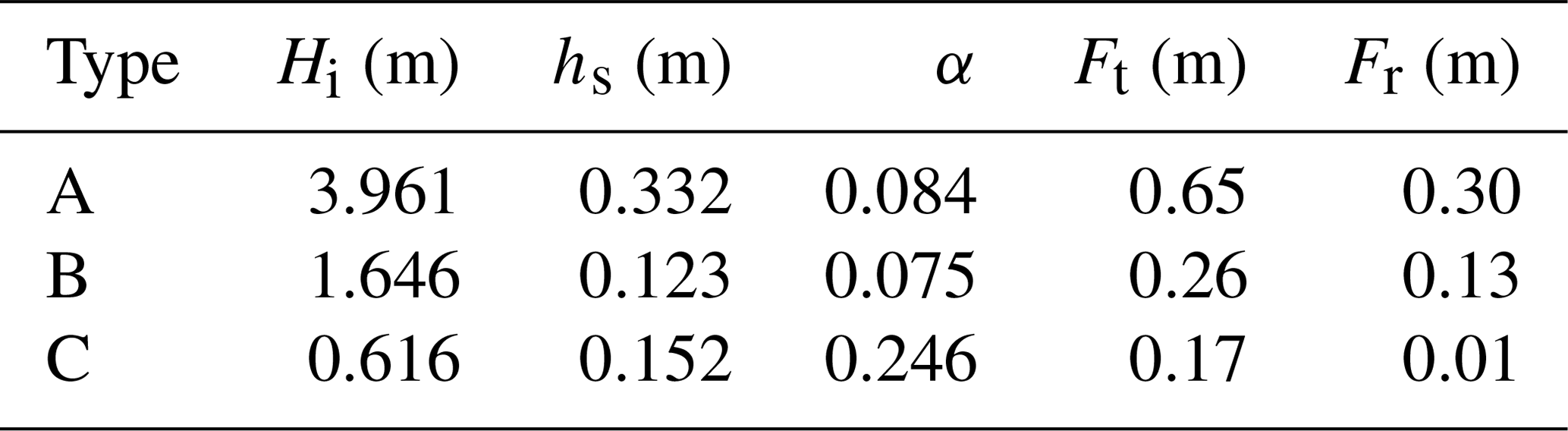
Table B2Errors of snow depth (Δhs) and ice thickness (ΔHi) for snow depth to ice thickness ratio error (Δα) of ±0.05.
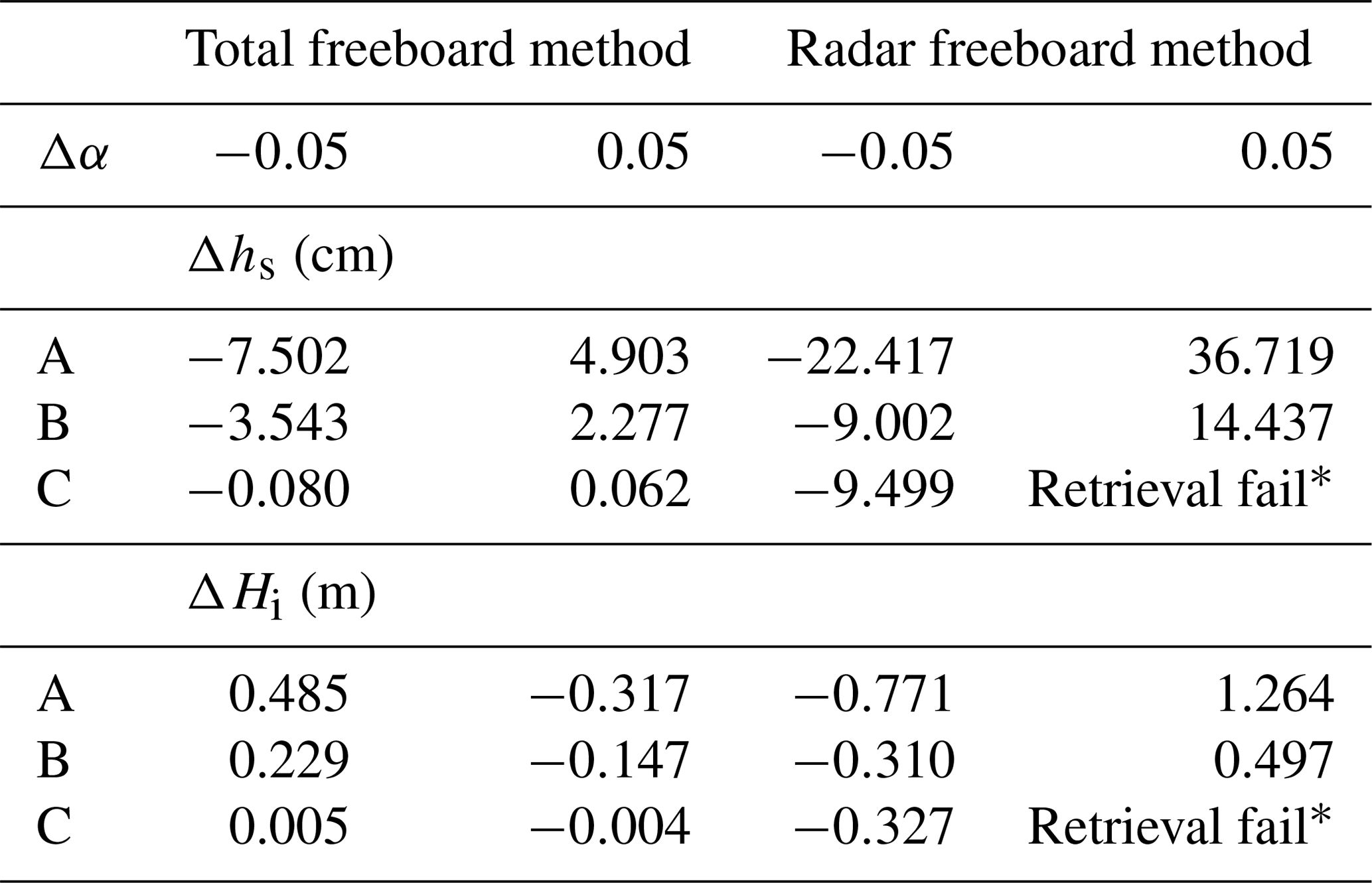
∗ Retrieval fail occurs if (αcrit=0.291 for ρs=320 kg m−3, ρI=915 kg m−3, ρw=1024 kg m−3, and f=0.84).
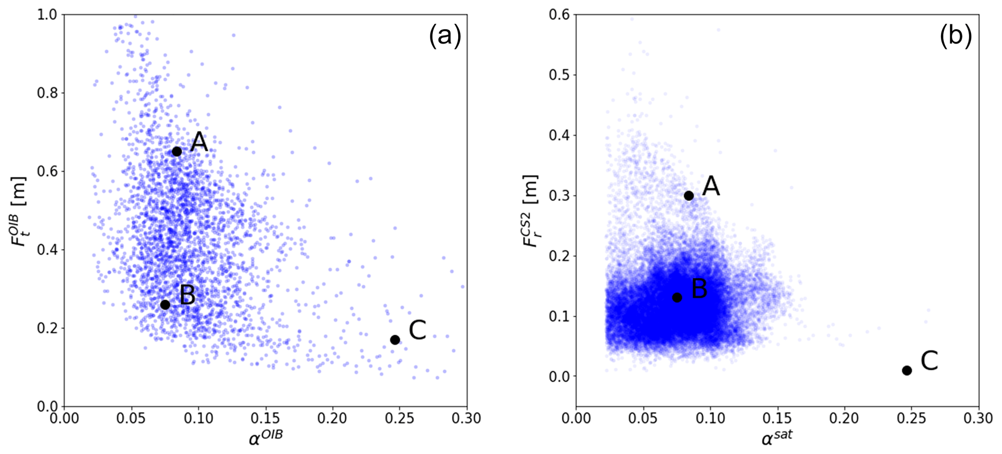
Figure B1Locations of physical states for typical types (A, B, C) on the freeboard-thickness ratio space. Blue dots are from (a) OIB data and (b) retrieved thickness ratio and CS2 radar freeboard.
Table B3Statistics of success/fail ratios of α retrieval for winter 2011–2015.
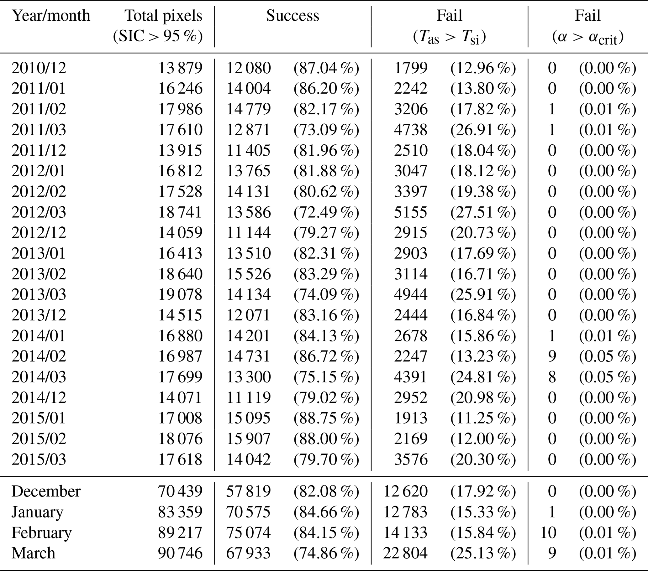
αcrit=0.291 for ρs=320 kg m−3, ρi=915 kg m−3, ρw=1024 kg m−3, and f=0.84.
Although the sensitivity test regarding uncertainty of satellite-derived α has been conducted in Appendix B, the uncertainty of CS2 freeboard measurements and prescribed parameters should be considered as well for the satellite snow depth and ice thickness estimates. To do so, a simple propagation analysis of errors is performed, regarding the uncertainty of satellite products (αsat and ) and prescribed parameters (ρi, ρs, and f). Uncertainty due to the variability of ρw is neglected (Kurtz and Harbeck, 2017; Hendricks et al., 2016; Ricker et al., 2014). Here we assume that αsat and are not correlated and have no systematic bias. Such an assumption may not be true in the real world. However, it allows us to estimate the retrieval uncertainty from satellite-derived products with a certain limit. Uncertainty of ice thickness can be estimated by the following Gaussian error propagation equation:
Here, εy,total denotes the total uncertainty of retrieved variable y (hs or Hi) and εy(x) denotes the uncertainty of y related to input variable x (α,Fr, ρi, ρs, or f). The uncertainties on the right-hand side are obtained by the following equation:
Here, σx denotes the uncertainty of x, and δ is set to be 10−6 for the numerical calculation of the partial derivative using Eqs. (3) and (12); σα is estimated to be an RMSD value between αOIB and αsat, σFr is given by Kurtz and Harbeck (2017), and σf is adopted from Armitage and Ridout (2015). Uncertainties of snow–ice densities are from the relevant literature (Alexandrov et al., 2020; Hendricks et al., 2016; Kern and Spreen, 2015; Ricker et al., 2014; Warren et al., 1999). Those values are summarized in Table C1.
Using Eqs. (C1) and (C2), uncertainties of snow depth and ice thickness retrievals can be estimated. Ice thickness uncertainty estimates are presented in Fig. C1. Total uncertainty of ice thickness estimates ranges from 0.8 to 2.0 m. Generally, Fr-related uncertainty in the third row is greater than α-related uncertainty in the second row. Snow depth uncertainty estimates are presented in Fig. C2. Total uncertainty of snow depths ranges from 0.04 to 0.4 m. In the case of the snow depth, α-related uncertainty is greater than Fr-related uncertainty. Both uncertainties of ice thickness and snow depth are greater for MYI regions than FYI regions. It is thought that the improvement of accuracy in satellite-derived temperatures can reduce the snow depth uncertainty, while the improvement of freeboard accuracy can reduce the ice thickness uncertainty. Uncertainties induced from densities and radar penetration factors are found to be relatively smaller than uncertainties related to α and Fr (shown in Figs. S2 and S3).
Table C1Values and uncertainties of input variables for uncertainty estimation.
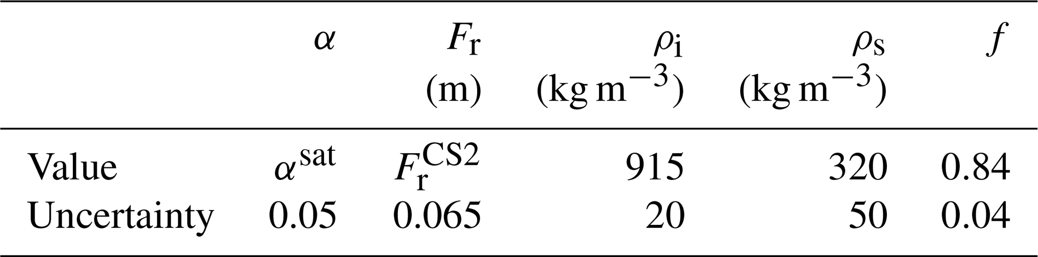
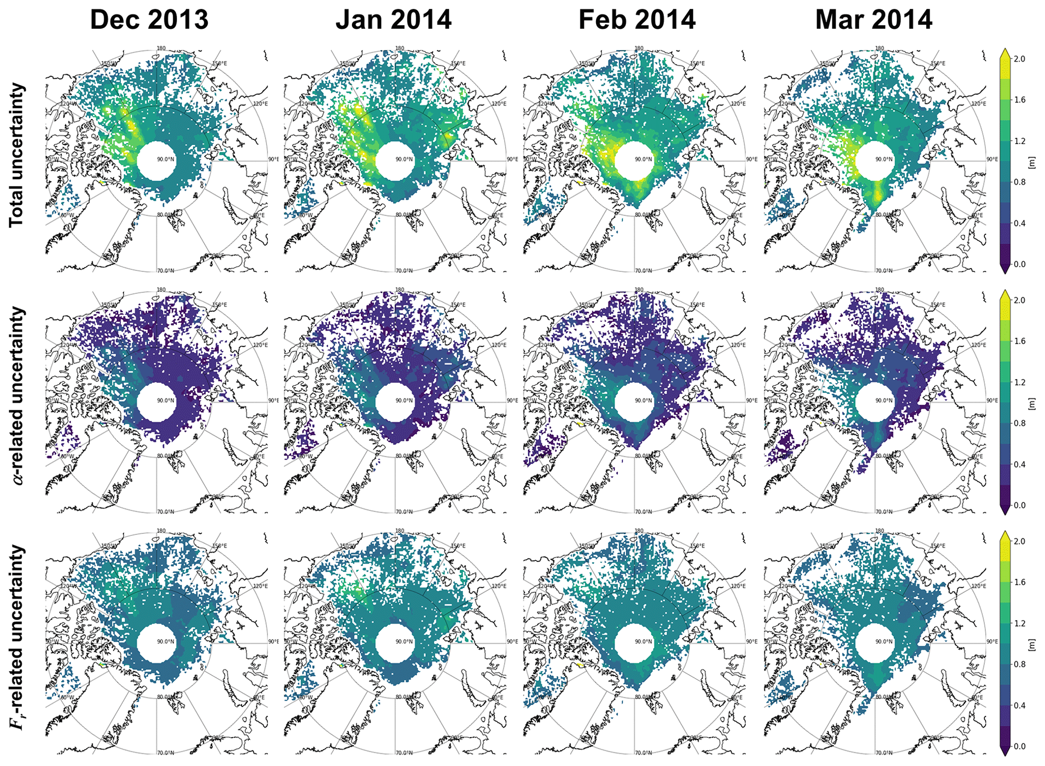
Figure C1Geographical distributions of sea ice thickness uncertainty: (first row) total uncertainty, (second row) α-related uncertainty, and (third row) Fr-related uncertainty for the period from December 2013 to March 2014.
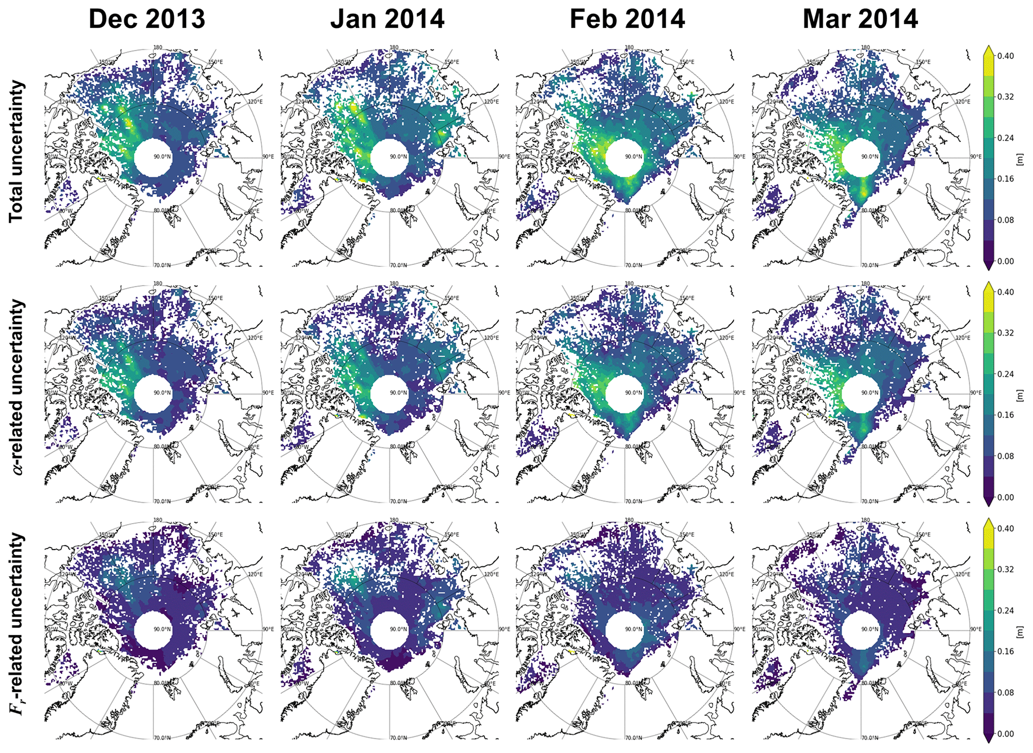
Figure C2Geographical distributions of snow depth uncertainty: (first row) total uncertainty, (second row) α-related uncertainty, and (third row) Fr-related uncertainty for the period from December 2013 to March 2014.
The SHEBA buoy data were obtained from NCAR/EOL (https://doi.org/10.5065/D6KS6PZ7, last access: 14 September 2020, Perovich et al., 2007), and CRREL-IMB buoy data were obtained from the CRREL-Dartmouth Mass Balance Buoy Program (http://imb-crrel-dartmouth.org, last access: 14 September 2019, Perovich et al., 2019). AASTI-v2 and SIIT data are available upon request to the authors. Other datasets were obtained from NSIDC. They are OIB data (https://doi.org/10.5067/G519SHCKWQV6, last access: 10 September 2019, Kurtz et al., 2015), OIB Quick Look data (https://doi.org/10.5067/GRIXZ91DE0L9, last access: 28 July 2020, Kurtz, 2019), CS2 data (https://doi.org/10.5067/96JO0KIFDAS8, last access: 10 September 2019, Kurtz and Harbeck, 2017), and SIC data (https://doi.org/ 10.5067/7Q8HCCWS4I0R, last access: 12 September 2019, Comiso, 2017).
The supplement related to this article is available online at: https://doi.org/10.5194/tc-14-3761-2020-supplement.
HS and BJS conceptualized and developed the methodology, and HS conducted data analysis and visualization. GD, RTT, and SML gave important feedback for the algorithm development and interpretation of results. GD provided AASTI data. All of the authors participated in writing the paper; HS prepared the original draft under the supervision of BJS and GD, and BJS critically revised the paper.
The authors declare that they have no conflict of interest.
We appreciate NSIDC for producing and providing the OIB, CS2, and SIC datasets. We also give thanks to CRREL and NCAR/EOL under the sponsorship of the National Science Foundation for providing IMB and SHEBA buoy data. The authors express their sincere thanks to an anonymous reviewer and to Isobel R. Lawrence for their valuable comments that led to the improvement of the paper.
This study has been supported by the Space Core Technology Development Program (NRF-25 2018M1A3A3A02065661) of the National Research Foundation of Korea and by Korea Meteorological Administration Research and Development Program under grant KMIPA KMI2018-06910. This study has also been supported by the International Network Program of the Ministry of Higher Education and Science, Denmark (grant ref. no. 8073-00079B).
This paper was edited by Yevgeny Aksenov and reviewed by Isobel Lawrence and one anonymous referee.
Alexandrov, V., Sandven, S., Wahlin, J., and Johannessen, O. M.: The relation between sea ice thickness and freeboard in the Arctic, The Cryosphere, 4, 373–380, https://doi.org/10.5194/tc-4-373-2010, 2010.
Armitage, T. W. K. and Ridout, A. L.: Arctic sea ice freeboard from AltiKa and comparison with CryoSat-2 and Operation IceBridge, Geophys. Res. Lett., 42, 6724–6731, https://doi.org/10.1002/2015GL064823, 2015.
Berg, W., Kroodsma, R., Kummerow, C. D., and McKague, D. S.: Fundamental Climate Data Records of Microwave Brightness Temperatures, Remote Sens., 10, 1306, https://doi.org/10.3390/rs10081306, 2018.
Braakmann-Folgmann, A. and Donlon, C.: Estimating snow depth on Arctic sea ice using satellite microwave radiometry and a neural network, The Cryosphere, 13, 2421–2438, https://doi.org/10.5194/tc-13-2421-2019, 2019.
Brucker, L. and Markus, T.: Arctic-scale assessment of satellite passive microwave-derived snow depth on sea ice using Operation IceBridge airborne data, J. Geophys. Res.-Oceans, 118, 2892–2905, https://doi.org/10.1002/jgrc.20228, 2013.
Comiso, J. C.: Bootstrap Sea Ice Concentrations from Nimbus-7 SMMR and DMSP SSM/I-SSMIS, Version 3, Boulder, Colorado USA, NASA National Snow and Ice Data Center, https://doi.org/10.5067/7Q8HCCWS4I0R, 2017.
Comiso, J. C., Cavalieri, D. J., and Markus, T.: Sea ice concentration, ice temperature, and snow depth using AMSR-E data, IEEE Trans. Geosci. Remote Sens., 41, 243–252, https://doi.org/10.1109/TGRS.2002.808317, 2003.
Cox, G. F. N. and Weeks, W. F.: Salinity variations in sea ice, J. Glaciol., 13, 109–120, https://doi.org/10.3189/S0022143000023418, 1974.
Dybkjær, G. and Eastwood, S.: Validation Report for the OSI SAF High Latitude L2 Sea and Sea Ice Surface Temperature, OSI-205, Version 1.1, OSI SAF, 30 pp., 2016.
Dybkjær, G., Eastwood, S., Borg, A. L., Højer, J., and Tonboe, R.: Algorithm theoretical basis document for the OSI SAF Sea and Sea Ice Surface Temperature L2 processing chain, OSI-205-a and OSI-205-b, Version 1.4, OSI SAF, 40 pp., 2018.
Dybkjær, G., Tonboe, R., Højer, J., and Eastwood, S.: Arctic and Antarctic snow and ice Surface Temperatures from AVHRR thermal Infrared satellite sensors, 1982-2015, in preparation, 2020.
Guerreiro, K., Fleury, S., Zakharova, E., Rémy, F., and Kouraev, A.: Potential for estimation of snow depth on Arctic sea ice from CryoSat-2 and SARAL/AltiKa missions, Remote Sens. Environ., 186, 339–349, https://doi.org/10.1016/j.rse.2016.07.013, 2016.
Guerreiro, K., Fleury, S., Zakharova, E., Kouraev, A., Rémy, F., and Maisongrande, P.: Comparison of CryoSat-2 and ENVISAT radar freeboard over Arctic sea ice: toward an improved Envisat freeboard retrieval, The Cryosphere, 11, 2059–2073, https://doi.org/10.5194/tc-11-2059-2017, 2017.
Hendricks, S., Ricker, R., and Helm, V.: User Guide – AWI CryoSat-2 sea Ice thickness data product (v1.2), https://doi.org/10013/epic.48201, 2016.
Karlsson, K.-G., Anttila, K., Trentmann, J., Stengel, M., Meirink, J. F., Devasthale, A., Hanschmann, T., Kothe, S., Jääskeläinen, E., Sedlar, J., Benas, N., van Zadelhoff, G.-J., Schlundt, C., Stein, D., Finkensieper, S., Håkansson, N., Hollmann, R., Fuchs, P., and Werscheck, M.: CLARA-A2: CM SAF cLoud, Albedo and surface RAdiation dataset from AVHRR data – Edition 2, Satellite Application Facility on Climate Monitoring (CM SAF), https://doi.org/10.5676/EUM_SAF_CM/CLARA_AVHRR/V002, 2017.
Kern, S. and Spreen, G.: Uncertainties in Antarctic sea-ice thickness retrieval from ICESat, Ann. Glaciol., 56, 107–119, https://doi.org/10.3189/2015AoG69A736, 2015.
Kern, S., Khvorostovsky, K., Skourup, H., Rinne, E., Parsakhoo, Z. S., Djepa, V., Wadhams, P., and Sandven, S.: The impact of snow depth, snow density and ice density on sea ice thickness retrieval from satellite radar altimetry: results from the ESA-CCI Sea Ice ECV Project Round Robin Exercise, The Cryosphere, 9, 37–52, https://doi.org/10.5194/tc-9-37-2015, 2015.
Kilic, L., Tonboe, R. T., Prigent, C., and Heygster, G.: Estimating the snow depth, the snow–ice interface temperature, and the effective temperature of Arctic sea ice using Advanced Microwave Scanning Radiometer 2 and ice mass balance buoy data, The Cryosphere, 13, 1283–1296, https://doi.org/10.5194/tc-13-1283-2019, 2019.
Kurtz, N.: IceBridge Sea Ice Freeboard, Snow Depth, and Thickness Quick Look, Boulder, Colorado USA, NASA National Snow and Ice Data Center, https://doi.org/10.5067/GRIXZ91DE0L9, 2016, updated 2019.
Kurtz, N. T. and Farrell, S. L.: Large-scale surveys of snow depth on Arctic sea ice from Operation IceBridge, Geophys. Res. Lett., 38, L20505, https://doi.org/10.1029/2011GL049216, 2011.
Kurtz, N. and Harbeck, J.: CryoSat-2 Level-4 Sea Ice Elevation, Freeboard, and Thickness, Version 1, Boulder, Colorado USA. NASA National Snow and Ice Data Center Distributed Active Archive Center, https://doi.org/10.5067/96JO0KIFDAS8, 2017.
Kurtz, N. T., Farrell, S. L., Studinger, M., Galin, N., Harbeck, J. P., Lindsay, R., Onana, V. D., Panzer, B., and Sonntag, J. G.: Sea ice thickness, freeboard, and snow depth products from Operation IceBridge airborne data, The Cryosphere, 7, 1035–1056, https://doi.org/10.5194/tc-7-1035-2013, 2013.
Kurtz, N. T., Galin, N., and Studinger, M.: An improved CryoSat-2 sea ice freeboard retrieval algorithm through the use of waveform fitting, The Cryosphere, 8, 1217–1237, https://doi.org/10.5194/tc-8-1217-2014, 2014.
Kurtz, N., Studinger, M., Harbeck, J., Onana, V., and Yi, D.: IceBridge L4 Sea Ice Freeboard, Snow Depth, and Thickness, Version 1, Boulder, Colorado USA. NASA National Snow and Ice Data Center, https://doi.org/10.5067/G519SHCKWQV6, 2015.
Kwok, R. and Cunningham, G. F.: Variability of Arctic sea ice thickness and volume from CryoSat-2, Philos. T. Roy. Soc. A, 373, 20140157, https://doi.org/10.1098/rsta.2014.0157, 2015.
Kwok, R. and Markus, T.: Potential basin-scale estimates of Arctic snow depth with sea ice freeboards from CryoSat-2 and ICESat-2: An exploratory analysis, Adv. Space Res., 62, 1243–1250, https://doi.org/10.1016/j.asr.2017.09.007, 2018.
Kwok, R., Cunningham, G. F., Wensnahan, M., Rigor, I., Zwally, H. J., and Yi, D.: Thinning and volume loss of the Arctic Ocean sea ice cover: 2003–2008, J. Geophys. Res.-Oceans, 114, C07005, https://doi.org/10.1029/2009JC005312, 2009.
Lawrence, I. R., Tsamados, M. C., Stroeve, J. C., Armitage, T. W. K., and Ridout, A. L.: Estimating snow depth over Arctic sea ice from calibrated dual-frequency radar freeboards, The Cryosphere, 12, 3551–3564, https://doi.org/10.5194/tc-12-3551-2018, 2018.
Laxon, S., Peacock, N., and Smith, D.: High interannual variablility of sea ice thickness in the Arctic region, Nature, 425, 947–950, https://doi.org/10.1038/nature02050, 2003.
Laxon, S. W., Giles, K. A., Ridout, A. L., Wingham, D. J., Willatt, R., Cullen, R., Kwok, R., Schweiger, A., Zhang, J., Haas, C., Hendricks, S., Krishfield, R., Kurtz, N., Farrell, S., and Davidson, M.: CryoSat-2 estimates of Arctic sea ice thickness and volume, Geophys. Res. Lett., 40, 732–737, https://doi.org/10.1002/grl.50193, 2013.
Lee, S.-M., Sohn, B.-J., and Kummerow, C. D.: Long-term Arctic snow/ice interface temperature from special sensor for Microwave imager measurements, Remote Sens., 10, 1795, https://doi.org/10.3390/rs10111795, 2018.
Maaß, N., Kaleschke, L., Tian-Kunze, X., and Drusch, M.: Snow thickness retrieval over thick Arctic sea ice using SMOS satellite data, The Cryosphere, 7, 1971–1989, https://doi.org/10.5194/tc-7-1971-2013, 2013.
Mallett, R. D. C., Lawrence, I. R., Stroeve, J. C., Landy, J. C., and Tsamados, M.: Brief communication: Conventional assumptions involving the speed of radar waves in snow introduce systematic underestimates to sea ice thickness and seasonal growth rate estimates, The Cryosphere, 14, 251–260, https://doi.org/10.5194/tc-14-251-2020, 2020.
Markus, T. and Cavalieri, D. J.: Snow depth distribution over sea ice in the Southern Ocean from satellite passive microwave data, Antarct. Res. Ser., 74, 19–39, 1998.
Markus, T., Neumann, T., Martino, A., Abdalati, W., Brunt, K., Csatho, B., Farrell, S., Fricker, H., Gardner, A., Harding, D., Jasinski, M., Kwok, R., Magruder, L., Lubin, D., Luthcke, S., Morison, J., Nelson, R., Neuenschwander, A., Stephen, P., Popescu, S., Shum, C. K., Schutz, B. E., Smith, B., Yang. Y., and Zwally, J.: The Ice, Cloud, and land Elevation Satellite-2 (ICESat-2): Science requirements, concept, and implementation, Remote Sens. Environ, 190, 260–273, https://doi.org/10.1016/j.rse.2016.12.029, 2017.
Maykut, G. A. and Untersteiner, N.: Some results from a time-dependent thermodynamic model of sea ice, J. Geophys. Res., 76, 1550–1575, https://doi.org/10.1029/JC076i006p01550, 1971.
Nandan, V., Geldsetzer, T., Yackel, J., Mahmud, M., Scharien, R., Howell, S., King, J., Ricker, R., and Else, B.: Effect of Snow Salinity on CryoSat-2 Arctic First-Year Sea Ice Freeboard Measurements, Geophys. Res. Lett., 44, 10419–10426, https://doi.org/10.1002/2017GL074506, 2017.
Perovich, D., Richter-Menge, J., and Polashenski, C.: Observing and understanding climate change: Monitoring the mass balance, motion, and thickness of Arctic sea ice, CRREL-Dartmouth mass balance buoy program, available at: http://imb-crrel-dartmouth.org, last access: 14 September 2019.
Perovich, D., Richter-Menge, J., Tucker, W., Elder, B., and Bosworth, B.: Snow and Ice Temperature Profiles, Version 1.0. UCAR/NCAR – Earth Observing Laboratory, https://doi.org/10.5065/D6KS6PZ7, 2007.
Pringle, D. J., Trodahl, H. J., and Haskell, T. G.: Direct measurement of sea ice thermal conductivity: no surface reduction, J. Geophys. Res.-Oceans, 111, C05020, https://doi.org/10.1029/2005JC002990, 2006.
Ricker, R., Hendricks, S., Helm, V., Skourup, H., and Davidson, M.: Sensitivity of CryoSat-2 Arctic sea-ice freeboard and thickness on radar-waveform interpretation, The Cryosphere, 8, 1607–1622, https://doi.org/10.5194/tc-8-1607-2014, 2014.
Rostosky, P., Spreen, G., Farrell, S. L., Frost, T., Heygster, G., and Melsheimer, C.: Snow depth retrieval on Arctic sea ice from passive microwave radiometers – improvements and extensions to multiyear ice using lower frequencies, J. Geophys. Res.-Oceans, 123, 7120–7138, https://doi.org/10.1029/2018JC014028, 2018.
Sturm, M., Holmgren, J., König, M., and Morris, K.: The thermal conductivity of seasonal snow, J. Glaciol., 43, 26–41, https://doi.org/10.3189/S0022143000002781, 1997.
Sturm, M., Perovich, D. K., and Holmgren, J.: Thermal conductivity and heat transfer through the snow on the ice of the Beaufort Sea, J. Geophys. Res., 107, 8043, https://doi.org/10.1029/2000JC000409, 2002.
Tilling, R. L., Ridout, A., and Shepherd, A.: Estimating Arctic sea ice thickness and volume using CryoSat-2 radar altimeter data, Adv. Space Res., 62, 1203–1225, https://doi.org/10.1016/j.asr.2017.10.051, 2018.
Tiuri, M., Sihvola, A., Nyfors, E., and Hallikainen, M.: The complex dielectric constant of snow at microwave frequencies, IEEE J. Ocean. Eng., 9, 377–382, 1984.
Tonboe, R. T., Pedersen, L. T., and Haas, C.: Simulation of the CryoSat-2 satellite radar altimeter sea ice thickness retrieval uncertainty, Can. J. Remote Sens., 36, 55–67, https://doi.org/10.5589/m10-027, 2010.
Trodahl, H. J., Wilkinson, S. O. F., McGuinness, M. J., and Haskell, T. G.: Thermal conductivity of sea ice; dependence on temperature and depth, Geophys. Res. Lett., 28, 1279–1282, https://doi.org/10.1029/2000GL012088, 2001.
Ulaby, F. T., Moore, R. K., and Fung, A. K.: Microwave remote sensing: Active and passive, Volume 3 – From theory to applications, 1986.
Warren, S. G., Rigor, I. G., Untersteiner, N., Radionov, V. F., Bryazgin, N. N., Aleksandrov, Y. I., and Colony, R.: Snow depth on Arctic sea ice, J. Climate, 12, 1814–1829, https://doi.org/10.1175/1520-0442(1999)012<1814:SDOASI>2.0.CO;2, 1999.
Webster, M. A., Rigor, I. G., Nghiem, S. V., Kurtz, N. T., Farrell, S. L., Perovich, D. K., and Sturm, M.: Interdecadal changes in snow depth on Arctic sea ice, J. Geophys. Res.-Oceans, 119, 5395–5406, https://doi.org/10.1002/2014JC009985, 2014.
Wingham, D. J., Francis, C. R., Baker, S., Bouzinac, C., Brockley, D., Cullen, R., Chateau-Thierry, P., Laxon, S. W., Mallow, U., Mavrocordatos, C., Phalippou, L., Ratier, G., Rey, L., Rostan, F., Viau, P., and Wallis, D. W.: CryoSat: a mission to determine the fluctuations in Earth's land and marine ice fields, Adv. Space Res., 37, 841–871, https://doi.org/10.1016/j.asr.2005.07.027, 2006.
Willatt, R., Laxon, S., Giles, K., Cullen, R., Haas, C., and Helm, V.: Ku-band radar penetration into snow cover on Arctic sea ice using airborne data, Ann. Glaciol., 52, 197–205, https://doi.org/10.3189/172756411795931589, 2011.
Zhou, L., Xu, S., Liu, J., and Wang, B.: On the retrieval of sea ice thickness and snow depth using concurrent laser altimetry and L-band remote sensing data, The Cryosphere, 12, 993–1012, https://doi.org/10.5194/tc-12-993-2018, 2018.
Zwally, H. J., Schutz, B., Abdalati, W., Abshire, J., Bentley, C., Brenner, A., Bufton, J., Dezio, J., Hancock, D., Harding, D., Herring, T., Minster, B., Quinn, K., Palm, S., Spinhirne, J., and Thomas, R.: ICESat's laser measurements of polar ice, atmosphere, ocean, and land, J. Geodyn., 34, 405–445, https://doi.org/10.1016/S0264-3707(02)00042-X, 2002.
Zygmuntowska, M., Rampal, P., Ivanova, N., and Smedsrud, L. H.: Uncertainties in Arctic sea ice thickness and volume: new estimates and implications for trends, The Cryosphere, 8, 705–720, https://doi.org/10.5194/tc-8-705-2014, 2014.
- Abstract
- Introduction
- Method
- Data
- Results
- Conclusions and discussion
- Appendix A: Physical interpretation of the piecewise linearity between α and ΔTsnow ∕ ΔTice
- Appendix B: Sensitivity test for the proposed method
- Appendix C: Uncertainty estimation for CS2 retrievals
- Data availability
- Author contributions
- Competing interests
- Acknowledgements
- Financial support
- Review statement
- References
- Supplement