Enhancing sea ice knowledge through assimilation of sea ice thickness from ENVISAT and CS2SMOS

Arctic sea ice extent has declined significantly over the past four decades, opening up the Arctic to shipping and resource extraction while also impacting wildlife and local communities. This has led to an increasing need for skillful sea ice predictions. We focus on furthering the understanding of the role that sea ice thickness plays in the skilfulness of seasonal Arctic sea ice predictions. We look at how observations of sea ice thickness can improve both sea ice reanalyses and predictions. We use the Norwegian Climate Prediction Model (NorCPM) with 1° horizontal resolution for the ocean and sea ice components and approximately 2° for the atmosphere and land components, which has previously assimilated ocean and sea ice concentration observations. We additionally assimilate two sea ice thickness products: CS2SMOS, and, for the first time in any study, ENVISAT. This allows us to produce a two-decade (2003–2023) reanalysis with sea ice thickness assimilation focusing on the Arctic Ocean. This reanalysis is then used to initialise and generate a series of year-long seasonal hindcasts for each season of the reanalysis. The reanalysis and hindcasts are compared to observations and other reanalyses to assess the impact of sea ice thickness observations. Assimilation of sea ice thickness data strongly improves the representation of sea ice thickness and volume, primarily in the central Arctic as well as the ice edge location. Although ENVISAT observations have greater uncertainties, the dataset still provides a useful impact on the model. For prediction, sea ice thickness initialisation reduces the model biases of thickness throughout the year as well as errors in the detrended anomalies. Ice thickness bias correction results in improvements in the representation of the ice edge location, i.e., the timing and extent of the summer melting. Thickness initialisation has little improvements for detrended sea ice extent anomalies, but yields some skill in the Beaufort Sea and Central Arctic during summer. Overall, we show the impact of sea ice thickness assimilation has a positive effect on prediction skill in NorCPM.

1 Introduction

In the Arctic, both the atmosphere and ocean have undergone dramatic warming trends over the satellite era (Przybylak and Wyszyński, 2020; Steele et al., 2008), and continue to experience warming much faster than the rest of the globe (Cohen et al., 2014), leading directly to sea ice loss (Dai et al., 2019). The sea ice loss in this region is having a strong impact on Arctic wildlife and habitats (Descamps et al., 2017). There are also wide-reaching effects on tourism, resource extraction and communities living in the Arctic (Arruda and Krutkowski, 2017). This has led to increasing interest in the study of Arctic sea ice and, in particular, of seasonal predictions, which aim to predict the sea ice on seasonal time scales. As the Arctic climate has warmed, the sea ice has not only retreated (Comiso et al., 2008; Stroeve et al., 2014b), but also thinned (Nghiem et al., 2007; Giles et al., 2008; Kwok, 2018). Much of the Arctic sea ice has gone from being perennial year-round to seasonal, with an increase in the length of the open-water season (Nghiem et al., 2007; Sumata et al., 2023). Such radical change also makes seasonal Arctic sea ice prediction more challenging.

The field of seasonal Arctic sea ice prediction emerged and rapidly developed within the past two decades, focusing on identifying and improving our understanding of the physical properties of sea ice, in order to improve the prediction of Arctic sea ice under a changing climate. This began with the first seasonal sea ice predictions using global climate models (GCM) and continued with prediction studies from a variety of research centres and institutes around the world (Wang et al., 2013; Chevallier et al., 2013; Peterson et al., 2015; Guemas et al., 2016; Bushuk et al., 2017; Kimmritz et al., 2019). The sea ice prediction network (SIPN) is at the centre of this field. The SIPN collects September sea ice extent (SIE) forecasts initialised from June, July and August and September into the Sea Ice Outlook (SIO) report (Stroeve et al., 2014a; Bushuk et al., 2024). At present, over 30 different research groups of polar scientists contribute to the SIPN, using dynamical or statistical approaches to produce these predictions. Idealistic model experiments in GCMs estimate that sea ice area and extent in the Arctic could be predictable between 12–48 months in advance, though predictability beyond 36 months is dominated by atmospheric forcing and not the initial conditions (Blanchard-Wrigglesworth et al., 2011a, b). Sea ice thickness (SIT) may be predictable up to 2 years in advance (Holland et al., 2011; Koenigk et al., 2012), and can be important for SIE predictions up to 2 years ahead (Tietsche et al., 2014) in an idealised framework.

The evolution of the Arctic sea ice is governed by the evolution of SIT distribution, and these changes come from two sources: dynamical and thermodynamical. Sea ice dynamics govern the movement of the sea ice either in space, or within the thickness distribution (commonly known as ridging). Thermodynamic changes in the sea ice are composed of melting (lateral, bottom and top melt) and freezing (congelation and frazil ice formation). SIT therefore is a key variable for modelling the sea ice state. SIT observations can substantially improve reanalysis estimates of thickness, with smaller impacts on other model variables such as sea ice concentration (SIC) and sea ice drift (SID), which has been shown in a number of sea ice reanalysis studies using different observational sources of thickness (Xie et al., 2018; Fritzner et al., 2019; Williams et al., 2023), and freeboard (Sievers et al., 2023). For prediction of SIE, correct SIT initialisation and its advection through the Arctic is believed to be one of the key mechanisms for skill within the Arctic (Blanchard-Wrigglesworth et al., 2011b; Ordoñez et al., 2018; Giesse et al., 2021; Zhang et al., 2021; Min et al., 2023; Zhang et al., 2023), and has been shown recently for CryoSat-2 (CS2) observations when using the CICE model standalone (Sun and Solomon, 2024). This is particularly true during the growth season which has been shown to translate to improved skill in SIE during the summer melt season (Blockley and Peterson, 2018; Holland et al., 2019). Additional mechanisms identified as important in the Arctic for SIE prediction are initialisation, persistence and re-emergence of SIC (Blanchard-Wrigglesworth et al., 2011b; Ordoñez et al., 2018; Giesse et al., 2021), ocean heat transport (OHT), ocean heat content (OHC) and melt onset timing (Schröder et al., 2014; Serreze et al., 2016; Kwok, 2018; Zheng et al., 2021). Atmospheric processes, particularly wind, which determine the dominant Arctic ocean currents of the Transpolar drift stream and the Beaufort Gyre, are also important but have a short memory, so its predictability can deteriorate quickly (Msadek et al., 2014; Serreze and Meier, 2019). Though several mechanisms have been identified in general, many are still poorly understood. In this paper, we will focus on improving thickness initialisation, and in doing so, using a longer period of SIT observations to study Arctic sea ice predictability.

In the past 15 years, significant work has been done on developing and producing new SIT observation datasets. At the forefront of this field are SIT datasets from CS2 (Laxon et al., 2013), available since October 2010, the combined CS2 and Satellite Moisture and Salinity (SMOS) dataset (Ricker et al., 2017) known as CS2SMOS. These datasets are the longest running available Arctic SIT observations, but until recently summer observations of SIT were not available due to the presence of melt ponds, though this has now changed with the work of Landy et al. (2022) to produce a year-round CS2 thickness dataset. The launch of ICESat-2 in 2018 also led to a winter SIT dataset using laser observations (Petty et al., 2020). However, before these satellites were launched, there were the forerunner satellites of ICESat (Kwok et al., 2004) and ENVISAT (Louet and Bruzzi, 1999). As they were not primarily designed for SIT retrieval, the datasets have issues, particularly with spatial and temporal coverage, and also the instruments used. Monthly observations of SIT have been derived from ENVISAT for the winter months not available during summer due to melt ponds, as with CS2 (Connor et al., 2009), which spans from October 2002 to 2012. In this work, we use the ENVISAT dataset to lengthen our reanalysis and increase the number of predictions possible for our statistical analysis.

In this study, we will investigate how assimilation of SIT observations from ENVISAT and CS2SMOS can first benefit our sea ice reanalysis and then summer Arctic sea ice predictions by using seasonal hindcasts (i.e. retrospective predictions) started from 2003 to 2023. To our knowledge, ENVISAT SIT observations have not been assimilated before in a GCM, so this study will investigate their use and feasibility of inclusion for assimilation in GCMs for the first time. As we use ENVISAT observations, this also means we have a longer time series of SIT observations to assimilate, and thus a longer reanalysis and more hindcasts with which we can analyse, study and verify its usefulness within these fields. We investigate not only SIE/SIT predictions but also the prediction of the sea ice edge location using the integrated ice edge error (IIEE).

The paper is organised as follows. In Sect. 2, we outline the climate model, observations and experimental design. In Sect. 3, we outline the metrics and independent observations used for evaluating and validating the performance of the model. In Sect. 4.1, we show the results of the sea ice reanalysis from 2003 to 2023, including verification of the reanalysis with independent data from the Beaufort Gyre Exploration Project (BGEP) moorings. In Sect. 4.2, we show the results of the hindcast experiments. In Sect. 5, we discuss the key results and conclude this study.

2 NorCPM

We use the Norwegian Climate Prediction Model (NorCPM, Counillon et al., 2016; Wang et al., 2019), which combines the Norwegian Earth System Model (NorESM Bentsen et al., 2013) and the Ensemble Kalman Filter (EnKF, Evensen, 1994) data assimilation method. The version of NorCPM is as in Kimmritz et al. (2019), which contributed to the SIPN (Bushuk et al., 2024), but we are testing, in addition, a separate version that assimilates ice thickness data.

2.1 NorESM

The NorESM version used here is NorESM1-ME (Bentsen et al., 2013). It is based on the Community Earth System Model (CESM, Hurrell et al., 2013). However, the ocean component is replaced with an isopycnal coordinate ocean general circulation model (BLOM, Bentsen et al., 2013), and the Community Atmosphere Model version 4 (CAM4, Neale et al., 2010) with the original prescribed aerosol formulation is replaced by the atmospheric model CAM4-OSLO with a prognostic aerosol life cycle formulation using emissions and new aerosol-cloud interaction schemes (Kirkevåg et al., 2013). As in CESM1.0.4, NorESM1-ME uses the Los Alamos Sea Ice Model version 4 (CICE, Hunke et al., 2015) and the Community Land Model (CLM) version 4 (Lawrence et al., 2011). These are coupled using version 7 of the coupler designed for the CESM (Craig et al., 2012).

The atmosphere and land model has an approximately 2° finite volume grid, with horizontal resolutions of 1.9° in latitude and 2.5° in longitude, while the ocean and sea ice have approximately a 1°×1° horizontal resolution. BLOM uses 51 isopycnal layers plus 2 additional layers for the bulk mixed layer, with time-evolving thicknesses and densities. This version of NorESM is run with CMIP5 historical forcings (Taylor et al., 2012) and the RCP8.5 (Moss et al., 2010) beyond 2005. A similar version of NorCPM has contributed to CMIP6 Decadal Climate Prediction Project (Bethke et al., 2021). However, upgrading to CMIP6 forcings degraded NorCPM's baseline climate and hindcast performance (Bethke et al., 2021; Passos et al., 2023), and we use CMIP5 forcings in this study.

The sea ice model CICE uses five categories in its thickness distribution, optimal for representing the sea ice cover at reasonable computing power (Bitz et al., 2001; Massonnet et al., 2019). The horizontal transport of sea ice is solved using an incremental remapping scheme (Lipscomb and Hunke, 2004), and solving for the sea ice stresses using the elastic-viscous-plastic rheology (Hunke and Dukowicz, 1997). The one-dimensional vertical Bitz and Lipscomb model (Bitz and Lipscomb, 1999), is used to solve the thermodynamic equations, with melt pond, aerosol (Holland et al., 2012) and radiation transfer parameterisations (Briegleb and Light, 2007). Sea ice transported in thickness space is solved using a remapping scheme (Lipscomb, 2001).

2.2 Assimilation implementation

The EnKF is a sequential ensemble data assimilation (DA) method using Monte Carlo integration followed by a linear analysis update (Evensen, 1994). The method is multivariate and updates the model state variables based on their ensemble covariances with the observations. Specifically, we use a deterministic formulation of the EnKF (Sakov and Oke, 2008), which solves the analysis without needing to perturb the observations. The Deterministic EnKF outperforms the standard EnKF, particularly for small ensemble sizes (Sakov and Oke, 2008).

We assimilate the monthly average observations in the middle of the model month (i.e., the 15th day) and update the instantaneous model state based on all observations (Counillon et al., 2016; Kimmritz et al., 2019). The update of the model state during the assimilation is split into two steps: the ocean model variables and the model variable SIC are updated jointly by the assimilation of oceanic and SIC observations, and then the model variable SIC is again updated by the assimilation of SIT observations. The atmosphere and land components are not updated by the assimilation but adjusted dynamically via coupling in between the monthly assimilation cycles.

Assimilation of ocean temperature and salinity profiles, sea surface temperature (SST), and SIC observations is performed as described in Kimmritz et al. (2019). We employ anomaly-field assimilation, using a monthly reference climatology calculated from 1982 to 2016. We update both the ocean and sea-ice components based on the observations from both components, so called strongly coupled ocean-sea ice DA (Laloyaux et al., 2016; Kimmritz et al., 2018). Strongly coupled ocean-sea ice DA in NorCPM was shown to be more effective than weakly coupled DA in which sea ice observations are used to only update the sea ice variables (Kimmritz et al., 2018). We update the full ocean physics state vector in isopycnal coordinates (i.e., 3D temperature, salinity, velocities and layer thickness) and update the multicategory SIC in the sea ice state vector (i.e., the multicategory aicen within the 5 categories, see DEPTH HI_PRESERVE in Kimmritz et al., 2018). The sea ice volume in each thickness category is changed proportionally so that the thickness of each thickness category remains identical to that of the prior ensemble (i.e., the multicategory hicen before assimilation). This prevents the need to reshuffle ice to a different thickness category in the post-analysis, which proved to be optimal in an idealised twin experiment (Kimmritz et al., 2018). The post-processing step ensures that sea ice state variables remain within physical ranges and recompute the energy budget of each of the multicategory sea ice quantities (Appendix 1 in Kimmritz et al., 2018, for further details). However, in Kimmritz et al. (2019), assimilation was carried out in 2 steps with SST and SIC updating the mixed layer depth ocean and the sea ice state, followed by assimilation of ocean profiles that update the full 3D ocean. This degraded performance in the lower latitudes where there are few profiles data to constrain the ocean interior. Therefore, we carry out a single assimilation step based on all observation products, which updates the full ocean and sea ice state jointly. This handled the degradation reported in Kimmritz et al. (2019) and has no impact on performance at high latitudes (not shown).

NorESM has a large SIT bias (Bentsen et al., 2013), and while assimilation of ocean observation reduces it partially, some of the bias remains. Bethke et al. (2021), compared two versions of NorCPM assimilating ocean observations, one that updates only the ocean component and one that updates the ocean and sea ice components. The latter yields a strong reduction of the bias of SIT and provides enhanced predictions. Note also that it takes about ten years for the model to rebuild the SIT bias once assimilation is stopped (their Fig. S15). We, therefore, use full-field assimilation to correct the SIT bias that can influence the variability. In the first attempt, we used anomaly-field assimilation (Carrassi et al., 2014). However, the assimilation impact of SIT anomalies was inconclusive, with no added skill for predictions (not shown).

When assimilating SIT observations, we only update the individual category sea ice fraction, which can change the sum of the ice fraction. In the post-processing of the assimilation, the sea ice volume in each thickness category is changed proportionally so that the thickness of each thickness category remains identical to that of the prior. We do not update the ocean component, as the covariances between SIT and the ocean are very small, and may cause more harm than benefit because of sampling error.

We use a series of ad-hoc techniques to handle issues related to sampling error, typically used in NorCPM (Counillon et al., 2016; Bethke et al., 2021). First, we used the R-factor (Sakov et al., 2012), which inflates the observation error by a factor of 2 for the update of the ensemble anomaly. We also use the K-factor formulation (Sakov et al., 2012), which inflates the observation error so that the analysis remains within m times the standard deviation of the ensemble (m=2 in this study). This avoids producing too strong updates. Finally, we use a local analysis framework (Evensen, 2003), which only uses the local observations and limits the risk of spurious covariance. Tapering with a smooth distance-weighted Gaspari and Cohn function (Gaspari and Cohn, 1999) ensures continuity in the update. The localisation radius for the ocean variables is a function of latitude (Wang et al., 2017), and for the SIC and SIT observations we use a localisation radius of 800 km as used previously (Kimmritz et al., 2018; Massonnet et al., 2015).

Our DA implementation assumes the observation errors to be independent. However, since observations of SST, SIC and SIT are gridded products, the observation error may be correlated due to heavy post-processing during data production. To mitigate this fact, we only retain the nearest observation of each observation type in the local analysis (Counillon et al., 2016; Kimmritz et al., 2018). For the hydrographic profiles, all data within the local window are used (Wang et al., 2017).

2.3 Assimilated datasets

SST and SIC monthly average data are from the NOAA OISSTV2 dataset (Reynolds et al., 2007; Huang et al., 2021) available on a 1°×1° global grid. The data is originally produced as weekly fields, NOAA then produces monthly fields using a linear interpolation of the weekly fields to daily fields then averaging those daily values over each month. The SST data are produced by combining both in-situ and satellite observations and SST's simulated by sea ice cover (Reynolds et al., 2007). Note that SST data in the regions covered by sea ice are not assimilated in this study (Kimmritz et al., 2019; Wang et al., 2019). However, the ocean underneath the sea ice is updated based on the ensemble covariance. Monthly SST observation errors are estimated using the weekly error estimation provided by the dataset. We experience that error in SST tends to be very low and we imposed a minimum threshold of 0.1 °C. SIC observation errors are not provided with the dataset and thus we use a 20 % constant value (Kimmritz et al., 2019), which is the generally agreed upon value for the highest uncertainties in the summer melt season (Ivanova et al., 2015; Cavalieri and Parkinson, 2012; Comiso, 2017).

The temperature and salinity profile data from October 2003 to October 2021 are taken from EN4.2.1 dataset (Gouretski and Reseghetti, 2010; Good et al., 2013). The data from then onwards are from EN4.2.2 dataset (Gouretski and Cheng, 2020). The EN4 hydrographic dataset is split into different categories depending on its quality. In this study, we only use data in category 1 (i.e., the highest quality). Their associated observation errors are determined as in Wang et al. (2017).

For the SIT observations, we use two datasets: the ESA CCI dataset that includes SIT retrieved from ENVISAT (Connor et al., 2009), and the AWI CS2SMOS dataset (V2.6) (Ricker et al., 2018) that retrieves SIT from the SMOS satellite and the CS2 satellite. The ESA CCI dataset covers the period from October 2002 to April 2012, however we only use data up to March 2010 because the more accurate CS2SMOS product becomes available after this. For both datasets, data is only available outside the melt season between October and April. Melt ponds on top of sea ice make it challenging to identify leads, which is crucial for the estimation of freeboard and SIT (Laxon et al., 2013). Additionally, we do not use October or April data due to certain quality issues associated with the fringe months marking the change between the melting and growth seasons in the Arctic sea ice. The observation error statistics are provided by the datasets.

2.4 Experiment design

In this work, we want to test the added value of SIT assimilation. For that, we have run several experiments. We use an ensemble model simulation without data assimilation and two reanalyses as follows:

FREE:

a 30-member ensemble run without data assimilation integrating from 1850 to December 2023 with CMIP5 historical forcings and with RCP8.5 beyond 2005. The ensemble is initialized on 1 January 1850 by randomly selecting 30 states on 1 January in different years from a stable pre-industrial run (with one single member).

CTRL:

A 30-member reanalysis started in 1982 branched from FREE (30 members), using a similar setting as in Kimmritz et al. (2019); Bushuk et al. (2024). It assimilates hydrographic profiles, SST, and SIC data (Sect. 2.3) with an anomaly-field assimilation framework.

+SIT:

a 30-member reanalysis is branched off from CTRL on the 15 October 2002. It assimilates SIT data (Sect. 2.3) in addition to that assimilated in CTRL.

FREE allows us to estimate the skill related to external forcings (Kimmritz et al., 2019). We use CTRL to compare the model with and without the assimilation of SIT data, while still assimilating the ocean and SIC observations. We use an ensemble size of 30 members primarily due to limited computational resources. In addition, many of the parameters in NorCPM (localisation, inflation) have been tuned to work ideally with an ensemble size of 30 which we found large enough to provide robust results for ocean and sea ice update with NorCPM (Counillon et al., 2014; Kimmritz et al., 2018).

Three sets of seasonal hindcasts (i.e., retrospective predictions) are created from FREE, CTRL and +SIT. They start on the 15th of January, April, July and October each year between 2003 and 2023 and run for 1 year with 10 members. This comprises 84 hindcasts in total (21 years and 4 hindcasts per year) for each set of hindcast experiments.

3 Validation metrics and datasets

We validate the reanalyses and hindcasts using their ensemble means. For the hindcast, we assess the performance for different start and lead months. Note that our hindcasts start in the middle of the month, but it has assimilated the monthly average of that month – e.g., our hindcast started on the 15 April has assimilated April monthly average data. Lead month 1 starts after 15 d of model integration (e.g., May is lead month 1 of April-initialised prediction).

We define the SIE as the total sum of the area of grid cells where the ensemble mean of SIC is at or above 15 %.

3.1 Validation metrics

We use bias and bias-free root-mean-square error (bfRMSE), defined as

$$\begin{array}{}\text{(1)}& {\displaystyle }\text{bias}& {\displaystyle }=\sum _{i=\mathrm{1}}^N{W}_i(x_i-y_i),\text{(2)}& {\displaystyle }\text{bfRMSE}& {\displaystyle }=\sqrt{\sum _{i=\mathrm{1}}^N{W}_i(x_i-y_i{)}^{\mathrm{2}}},\end{array}$$

where N is the total number of data points, W_i is a normalising area-based weight constant – i.e. when the metric is computed considering grid cells that do not have the same area. For point-wise bias and bfRMSE calculations, W_i is $\frac{\mathrm{1}}{N}$. x_i is the model ensemble mean values, and y_i is the observed values, which are both anomalies from their respective climatology (model or observation). These are usually averaged either over time or space (where each grid cell is then weighted by its area). Note that root-mean-square error (RMSE) is the quadratic sum of bias and bfRMSE.

We additionally use anomaly correlation coefficient (ACC) to test the variability of the reanalyses/hindcasts and the observations, defined as follows:

$$\begin{array}{}\text{(3)}& \text{ACC}={\displaystyle \frac{{\sum }_{i=\mathrm{1}}^N{x}_i^{\prime }{y}_i^{\prime }}{\sqrt{{\sum }_{i=\mathrm{1}}^N{x_i^{\prime }}^{\mathrm{2}}}\sqrt{{\sum }_{i=\mathrm{1}}^N{y_i^{\prime }}^{\mathrm{2}}}}},\end{array}$$

where $x_i^{\prime }$ and $y_i^{\prime }$ are model and observation values. For the reanalysis, we use the standard ACC and bfRMSE, but for the predictions, we use the detrended values – i.e. both time series are detrended before computing the metric. The reason is that the trend in reanalysis is part of the signal that one aims to represent and can be challenging due to discontinuity in the observation data set or drift in the system. In prediction, the trend is often removed as it is considered to be a trivial predictor (Bushuk et al., 2020). The statistical significance of the Pearson correlation coefficient is tested by using the Student's t test with a significant level of 5 % with degrees of freedom calculated as in Von Storch and Zwiers (2002).

The Degrees of Freedom for Signal (DFS) is calculated for each set of assimilated observations in the analysis to test the impact of their assimilation (Wahba et al., 1995; Cardinali et al., 2004).

$$\begin{array}{}\text{(4)}& \text{DFS}=\sum _{i=\mathrm{1}}^L{\displaystyle \frac{\partial x_a}{\partial y}},\end{array}$$

where L is the total number of observations and x_a is the model posterior. The DFS metric quantifies how the assimilation of observations has reduced the dimension or rank of the ensemble (Sakov et al., 2012). A larger DFS value implies that the assimilation has more change into the system, i.e., reducing the number of degrees of freedom (the unit of the metric). The DFS can be between 0 (no impact) and the total number of degrees of freedom minus one (where all members collapse to a single member)¹. A well-balanced data assimilation system aims to make minimal changes necessary to comply with observations, and as such, one should reach neither the lower nor the upper DFS value. As a consequence, DFS is often used to calibrate the strength of the data assimilation system when observation error is poorly known (Sakov et al., 2012) – prevent too strong or too weak assimilation. DFS can also be used to isolate the relative influence of each observation on the total impact of the assimilation, which is our aim in this study. More specifically, DFS is used here to diagnose the relative influence of the SIT assimilation compared to other datasets, for instance, where it is most beneficial, as well as to quantify the impact of ENVISAT SIT versus C2SMOS.

Finally, we use the Integrated Ice Edge Error (IIEE) to assess the error in the location of the ice edge (Goessling et al., 2016). It is defined as

$$\begin{array}{}\text{(5)}& \text{IIEE}=\underset{A}{\int }max(c_x-c_y,\mathrm{0})\mathrm{d}A+\underset{A}{\int }max(c_y-c_x,\mathrm{0})\mathrm{d}A,\end{array}$$

where A is the area, c=1 where the SIC is above 15 % and 0 elsewhere, with subscripts x and y denoting the model and observations respectively. This works as essentially the sum of all areas where SIE is overestimated (first term on right hand side (RHS) of the above equation) and underestimated (second term). The IIEE can also be decomposed in a different way, using a mean absolute error (MAE) and a displacement (DISP). This is formulated in Goessling et al. (2016) as

$$\begin{array}{}\text{(6)}& {\displaystyle }\text{IIEE}& {\displaystyle }=\text{MAE}+\text{DISP}\text{(7)}& {\displaystyle }\text{MAE}& {\displaystyle }=\mathrm{|}\text{O}-\text{U}\mathrm{|}\text{(8)}& {\displaystyle }\text{DISP}& {\displaystyle }=\mathrm{2}\cdot min(\text{O},\text{U}),\end{array}$$

where O is the area where SIE is overestimated, and U is the area where SIE is underestimated. The IIEE is a useful verification metric because it is conceptually simple. It is well verified with existing long-term SIC satellite data, is an important characteristic of the sea ice cover and is more useful to potential forecast users than total SIE (Goessling et al., 2016).

3.2 Independent validation datasets

In the paper, a part of the validation will be carried out with the assimilated dataset. In the reanalysis, such data cannot be considered independent, but still represents a baseline verification (that DA works as expected).

We use observations of sea ice draft from the BGEP moorings for independent validation. BGEP includes upward-looking sonar (ULS) measuring instruments (Krishfield et al., 2014). There are a total of 4 moorings, 2 of which (A and B) have been in operation since August 2003, C was in operation until 2008, and D has been in operation since 2005. All moorings are located in the Beaufort Sea (their location in the Arctic is shown in Fig. 3c). The ULS instruments measured sea ice draft every 2 s before 2014, and every second after. The sea ice draft, which is the thickness of the sea ice under sea level, is found by subtracting the range measured by the ULS instrument from the known depth of the instrument. The draft measurements have a stated error of ±5–10 cm (Krishfield and Proshutinsky, 2006). To compare this data to our model monthly mean thickness, we first convert the sea ice draft into SIT using the method of Rothrock et al. (2008), and then average all the measurements over each month or year to convert to monthly or yearly averages respectively, which we can compare to the model. If there was missing data in a month, we discard the ULS data for that month for that mooring, if there were more than thirty days of missing continuous data in a year, we do not compute a yearly average for that year.

The Pan-Arctic Ice Ocean Modeling and Assimilation System (PIOMAS) reanalysis was first introduced in 2003 by Zhang and Rothrock (2003). PIOMAS is a coupled ice-ocean model that assimilates SST data in ice-free grid cells using optimal interpolation, and SIC using a relatively simple nudging technique which aims to move the model variables closer to their observed counterparts by use of a weighting factor. PIOMAS has been substantially validated with a large number of SIT observations (Schweiger et al., 2011), so is often used as a comparison dataset for other SIT and sea ice volume datasets. The PIOMAS reanalysis is used for validation in this study.

4 Results

4.1 Reanalysis

In this section, we analyse our 21 year reanalyses over the period where satellite SIT observations are available.

In Fig. 1, we present the time evolution of the assimilation diagnostic. We can first notice that the bias has a seasonal signal that relates to the lack of observation during summer, when the bias increases. For ENVISAT, the system is too thick at the start but gets too thin at the end of the season, while with C2S the too thick bias remains positive until the end of the seasonal observation period. In an ensemble data assimilation system, one can use the ensemble spread as a measure of the system's error. A first check to assess the reliability of the system is to ensure that the quadratic sum of the ensemble standard deviation and observation error (here denoted as total error) matches the bias-free error of the ensemble mean (RMSE, Rodwell et al., 2016). We can notice that our system exhibits too high dispersion during the ENVISAT period, but that the reliability is very good in the C2S period. The overdispersion during the ENVISAT may relate to the observation error, which is very high. We can also notice that the ensemble spread and RMSE covary in time very well (both seasonally and inter-annually). There is a discrepancy at the start of the assimilation season that relates to the bias being large (not to be accounted for in the reliability budget analysis).

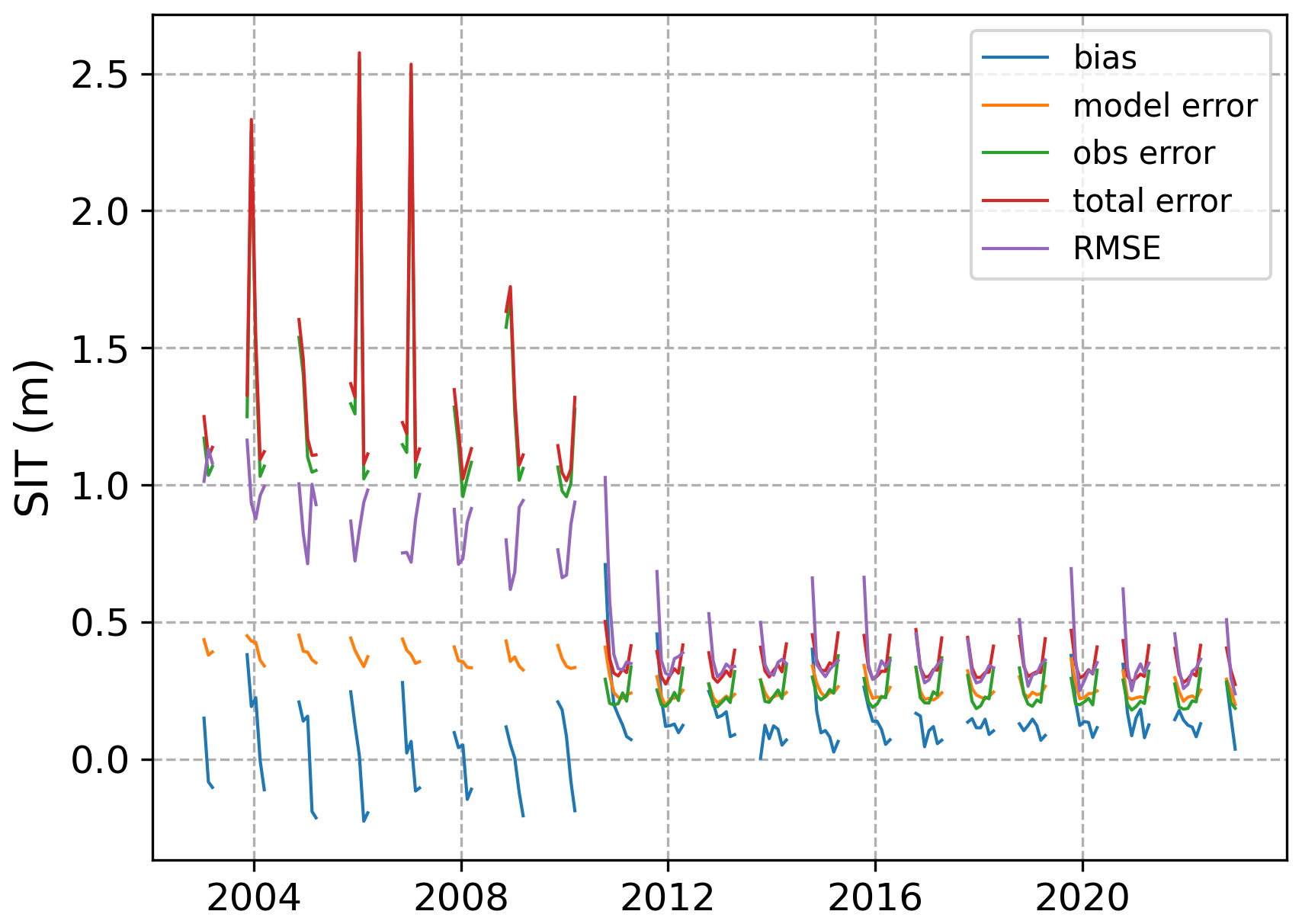
Figure 1 The time evolution of five key metrics of the EnKF for SIT assimilation (computed on the innovation vector – the difference between the observation and the model at the observation location): which is the bias, model error (ensemble standard deviation), observation error (standard deviation), total error (quadratic sum of model error and observation error) and RMSE. Note that there are gaps in the figure due to the lack of SIT observations outside winter.

We start by analysing the relative influence of each observation type in constraining errors in the system with the DFS (Sect. 3.1). The observations assimilated complement each other quite well and dominate in different regions (Fig. 2). The ocean observations dominate in the sea ice-free regions of the Arctic. SIC assimilation is most impactful at the sea ice edge, where SIC shows the largest variability. SIT assimilation is mainly effective in the central Arctic, where the ice is thicker. As expected, the SIT assimilation becomes more effective (higher DFS) when we switch over from assimilating ENVISAT to CS2SMOS. However, ENVISAT assimilation is still having a substantial impact in the central Arctic according to the DFS, where other observations are few, or have limited impact.

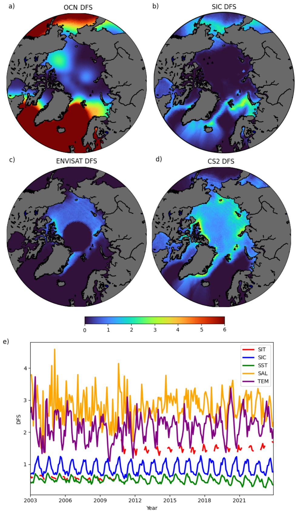
Figure 2 (a) Combined mean DFS of salinity, ocean temperature and sea surface temperature. (b) Mean DFS of SIC. (c) Mean DFS of ENVISAT SIT. (d) Mean DFS of CS2 SIT. (e) Pan-Arctic monthly mean DFS for each observation assimilated in our +SIT reanalysis. TEM refers to (ocean) temperature and SAL refers to salinity.

We first verify performance against the SIT observations (Fig. 3), which is assimilated in +SIT. We only present the validation against the CS2SMOS period due to the differing regional coverage between ENVISAT and CS2SMOS, but the conclusions are similar for ENVISAT (not shown). FREE has a clear thick bias (up to 4 m), with the spatial pattern of the bias increasing as the ice gets thicker – largest close to the Canadian Arctic Archipelago (CAA). In CTRL, the biases in the central Arctic Ocean have been reduced, but there is still a thin strip of too-thick sea ice pushed against the CAA. In +SIT the thickness biases in the marginal seas surrounding the central Arctic have almost been completely removed, which showcases the influence of assimilating ice thickness data.

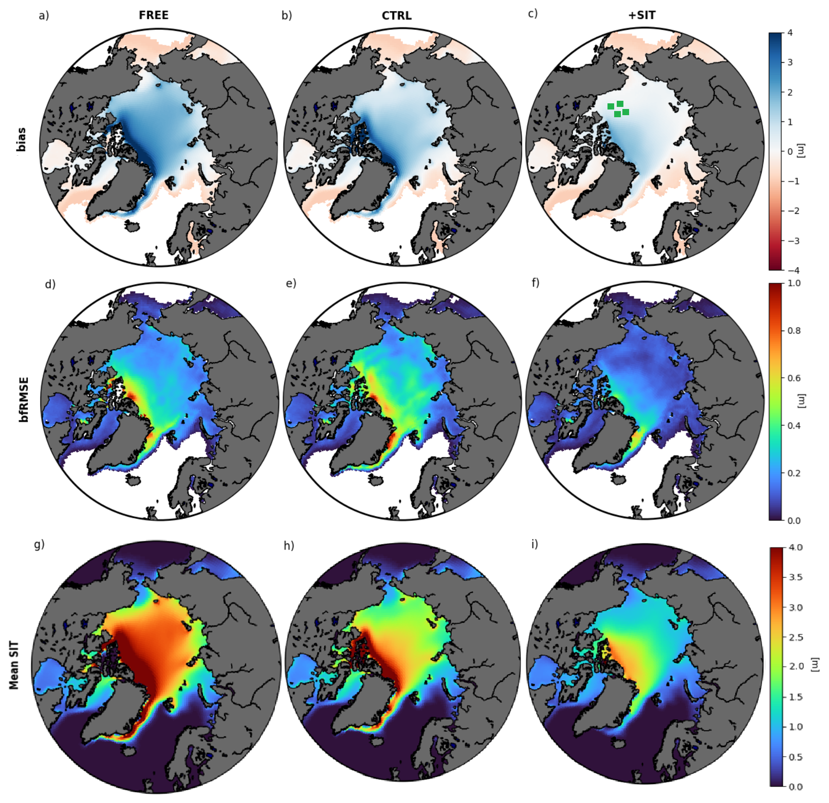
Figure 3 Bias (a–c), bfRMSE (d–f) and mean (g–i) of SIT in each of our NorCPM experiments in comparison to SIT observations from CS2SMOS between 2010 and 2023. In panel (c) we also show the locations of the BGEP ULS moorings as green squares.

For bfRMSE, FREE features errors of around 20 cm in a majority of places, reaching errors up to 1 m close to the CAA. Surprisingly, the SIT bfRMSEs are increased in CTRL in much of the central Arctic compared to FREE. This suggests that the assimilation of SIC and ocean observations has led to increased bfRMSEs for SIT. However, as the bias is much larger than bfRMSEs, the increased bfRMSEs result more from the evolution of the SIT bias in between and during the assimilation (the total RMSE is reduced). In the +SIT reanalysis, almost all grid cells feature low bfRMSE, especially in the central Arctic and CAA. There remain higher errors in the Fram Strait – albeit weaker than for FREE and CTRL – that are typically driven by sea ice export (Sumata et al., 2015). In this region, SIT observation errors are very large, and SIT assimilation effectiveness is reduced (Fig. 2). EXP-OCT performs better than EXP-OC against SMOS for the April–June period, while EXP-OC performs better against SMOS for the July–September period, with little differences in October.

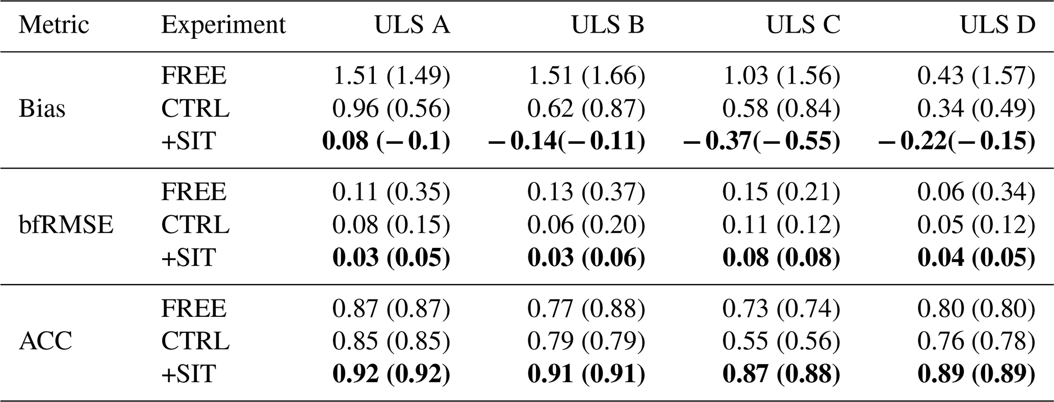
The previous comparison was done against assimilated observations of CS2SMOS, and we now compare with SIT derived from the independent BGEP moorings (Sect. 3.2). The moorings are all located in the Beaufort Gyre (Fig. 3c), so do not provide an assessment over the whole pan-Arctic region. The comparison (Fig. 4 and Table 1) is well in line with the above CS2SMOS validation. FREE has the largest biases (as high as 1.5 m); CTRL has smaller biases than FREE due to ocean and SIC assimilation. +SIT has the smallest biases among the three reanalyses. FREE has bfRMSE from 0.06 to 0.15 m, varying with the mooring and ACC around 0.7–0.8 as it captures the decreasing trends well with yearly data and the seasonal cycle with monthly outputs. The assimilation of the ocean and SIC data reduces bfRMSE (CTRL in Table 1) but yields a slight degradation of ACC at stations C and D. Assimilating SIT further reduces bfRMSE consistently with Fig. 3 and improves correlation (about 0.9). Overall, +SIT shows the best performance for all four moorings and performance is better during the CS2SMOS observations period than during the ENVISAT period.

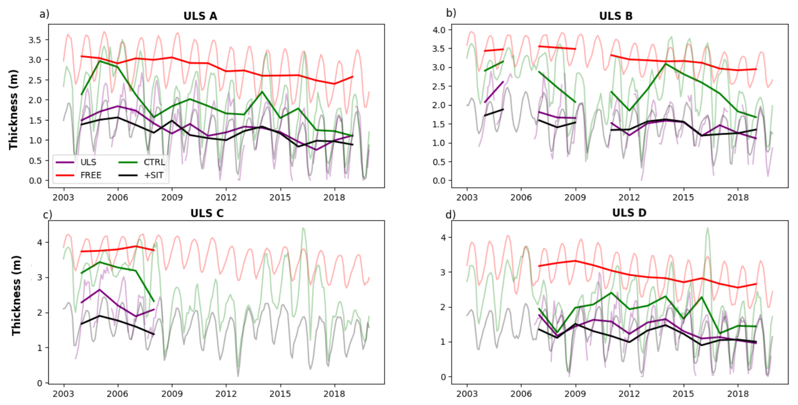
Figure 4 Yearly (thick line) and monthly (thin line) average sea ice thickness at ULS A (top left), B (top right), C (bottom left) and D (bottom right) and the respective SITs in our reanalyses during our experimental period. In some years, there are not enough observations (more than 30 d continuous of observations missing) from a ULS mooring to formulate a yearly average, so these years are masked.

Table 1 Bias, ACC and bfRMSE for the SIT of BGEP ULS A, B, C and D in comparison with the FREE, CTRL and +SIT reanalyses. The statistics are based on monthly mean detrended data. The statistics with yearly data are given in brackets. The unit of bias and bfRMSE is the metre. The system with the best performance are highlighted in bold.

We further analyse the seasonal variability of error of SIT and SIE (Fig. 5). There is little difference between the reanalyses in the bias of SIE (Fig. 5a) as we use an anomaly-field assimilation framework for ocean and SIC, which takes the climatology of FREE as an attractor. CTRL shows lower SIE bias than FREE in the ice-retreat season but slightly larger biases in the ice-advance season. SIE bias is substantially reduced in +SIT between April and September, and similar to FREE in the rest of the year.

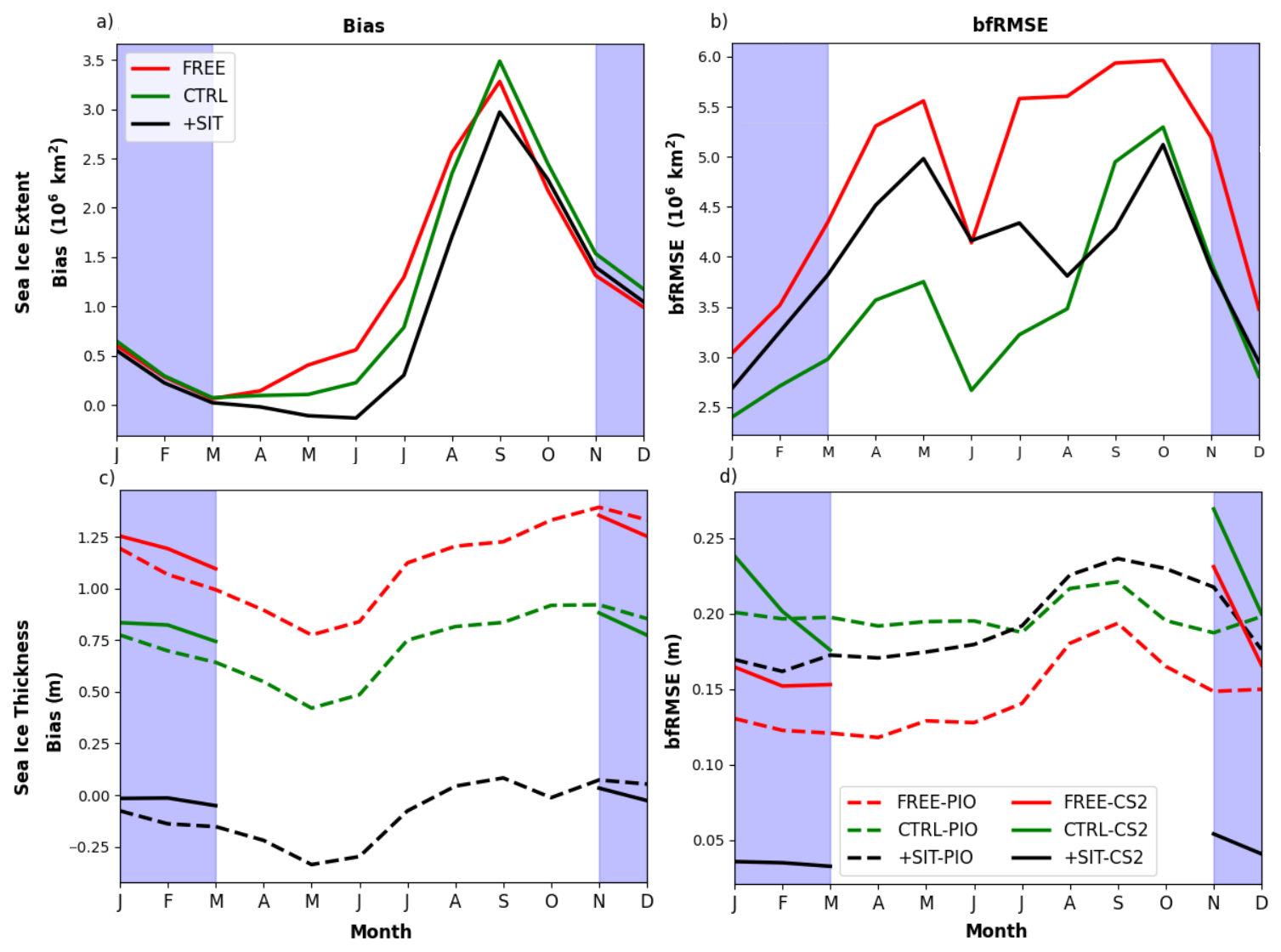
Figure 5 Bias (left-hand side) and bfRMSE (right-hand side) for SIE (top) and SIT (bottom) for FREE, CTRL and +SIT. SIC observations compared to SIC observations from NOAA, and the SIT from the PIOMAS reanalysis between 2003 and 2023 and CS2SMOS observations between 2010–2023. The blue-shaded area shows the time when SIT observations are assimilated.

For bfRMSE of SIE (Fig. 5b), +SIT and CTRL have lower errors than FREE, showing the positive impact of the assimilation of ocean and SIC data. However, the bfRMSE in SIT+ is larger than CTRL from January to August.

CTRL reduces the SIT bias compared to FREE uniformly throughout the year, and +SIT nearly removes entirely the SIT biases (Fig. 5c), even outside of the assimilated season when compared to PIOMAS. The bfRMSE is slightly increased in CTRL compared to FREE, likely for the same reason explained above, i.e. bfRMSE being lower than bias can be misleading. bfRMSE in SIT+ is interesting because it is very low when computed against CS2SMOS (Fig. 5d), but larger than FREE when computing bfRMSE against PIOMAS. PIOMAS tends to underestimate the interannual variability of SIT because it overestimates the thickness of thin ice and underestimates the thickness of the thick ice (Schweiger et al., 2011; Wang et al., 2016). As such, the ensemble mean of FREE, which is nearly indistinguishable from the linear decline, compares favourably with PIOMAS for bfRMSE.

We then investigate the time evolution of the SIE and SIV throughout the reanalysis for March and September (Fig. 6 and Table 2) when SIE reaches a maximum and minimum.

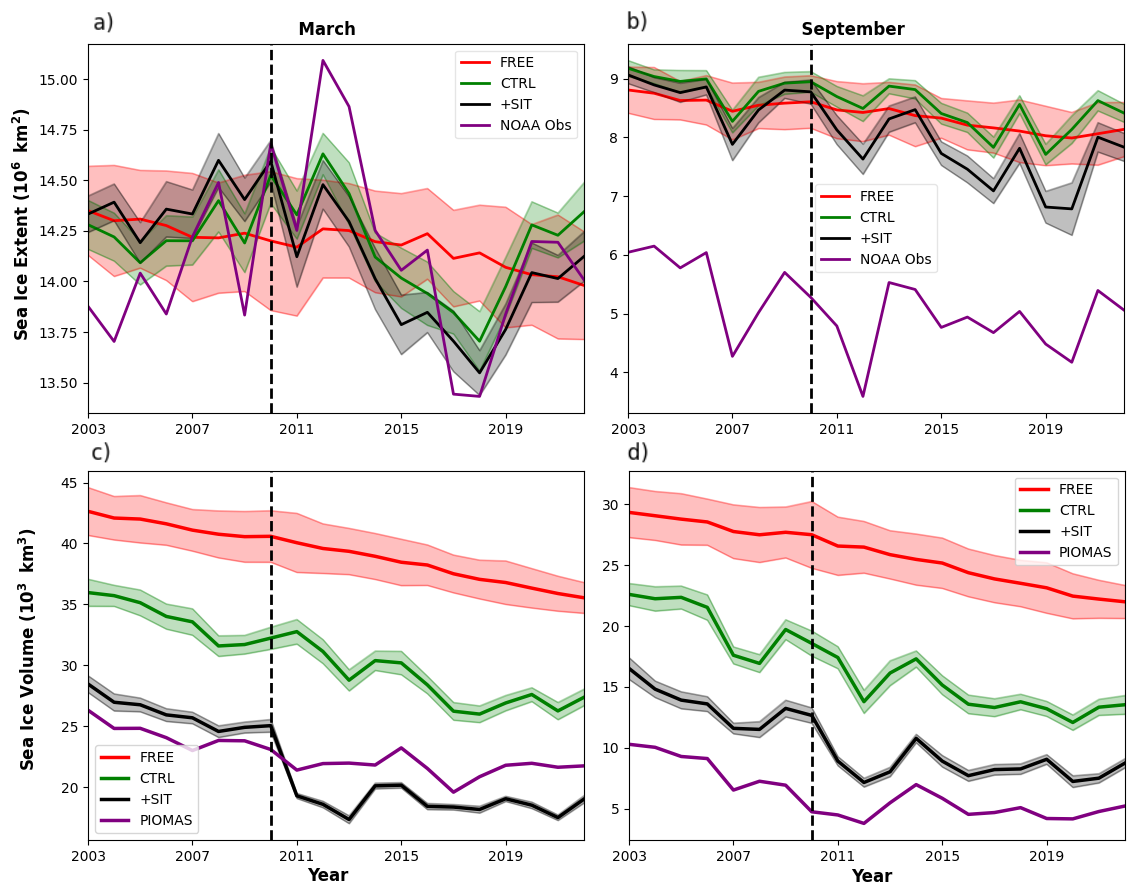
Figure 6 Arctic SIE (top) and SIV (bottom) in March (left-hand side) and September (right-hand side) for validation datasets and our experiments (FREE, CTRL and +SIT). Shaded region shows the ensemble mean plus/minus one standard deviation for each experiment. SIC observations from NOAA, and the SIV from the PIOMAS reanalysis between 2003 and 2023. The dashed vertical lines split the whole period to the ENVISAT and C2SMOS eras.

Table 2 Bias, bfRMSE and ACC for the SIE and SIV in March and September in the FREE, CTRL and +SIT experiments. The unit of bias and bfRMSE in SIE (SIV) is km² (km³). Observed SIE is computed from NOAA OISSTV2 and we use SIV computed from PIOMAS. The system with the best performance is highlighted in bold.

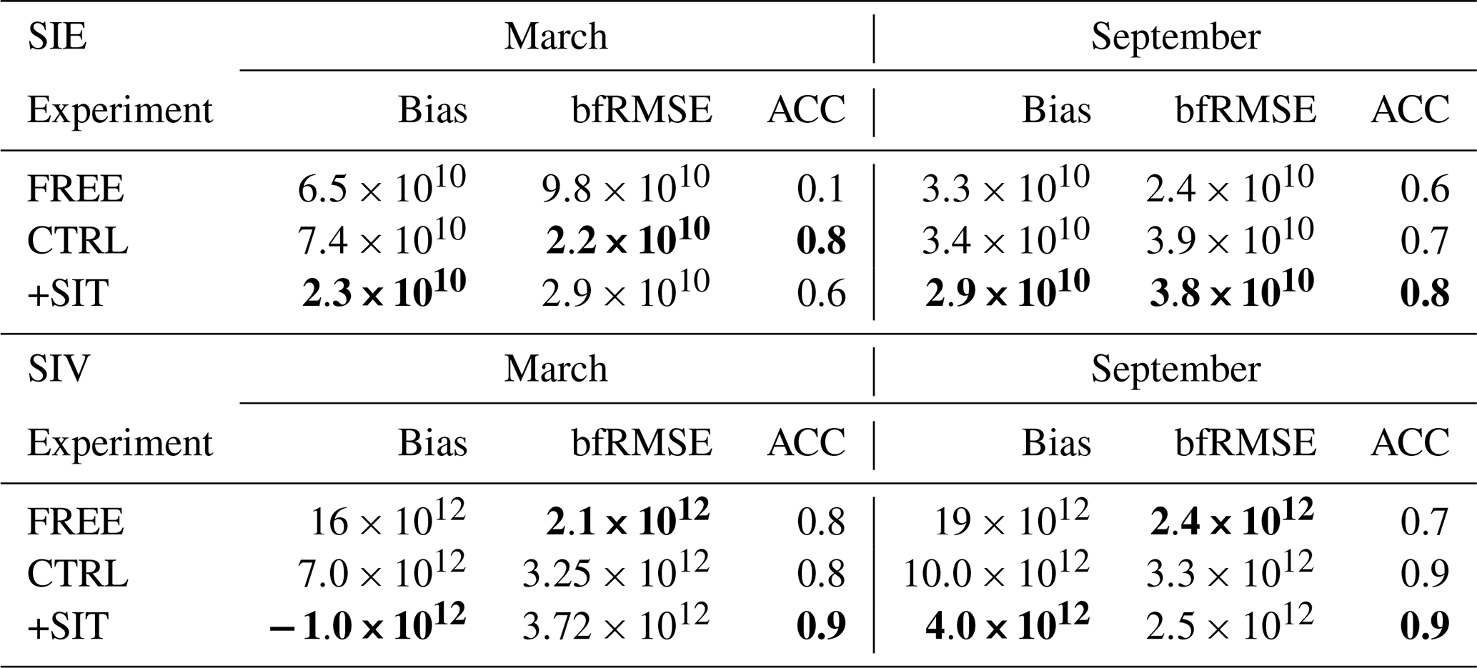
In March, FREE shows a weak decreasing trend in agreement with the observation but no year-to-year variability (as internal variability is not synchronised). CTRL shows good agreement with the assimilated NOAA observation estimate. Interannual variability is also much larger, implying that the individual members of CTRL are better constrained. +SIT also shows improved agreement with observations (amplitude of internal variability and ACC). The SIE bias is reduced from 7.4×10¹⁰ to 2.3×10¹⁰ km² by the SIT assimilation. ACC and bfRMSE of SIE are slightly degraded compared to CTRL (albeit better than FREE). This primarily relates to a spurious increasing trend until 2010 during the ENVISAT SIT observation period (Fig. 6a). The performance of ACC and bfRMSE for +SIT is comparable to CTRL in the C2SMOS era (not shown). All systems capture the decreasing trend in SIV well. Interannual variability is stronger in CTRL than in FREE and even more pronounced in +SIT (Fig. 6d). Despite some visual agreement in CTRL, ACC and bfRMSE are not improved compared to FREE. +SIT reduces the bias but has a larger bfRMSE than CTRL when compared to PIOMAS. Still, ACC is improved, and Fig. 5d suggests that PIOMAS underestimates interannual variability (quarrelling results for bfRMSE depending on whether we use C2SMOS or PIOMAS). +SIT has a strong discontinuity in 2010 for SIV during the transition between ENVISAT and C2SMOS.

In September, all systems have high positive SIE biases as a direct consequence of anomaly assimilation, as seen in Fig. 6. Table 2 shows that CTRL and +SIT show higher ACC values than FREE. The agreement is better in +SIT, with ACC increasing from 0.7 to 0.8, and slightly reduced bfRMSE. In Fig. 5, the ensemble mean of FREE shows, again, nearly no interannual variability. In the same figure, we see that +SIT better captures the amplitude of the peaks and, in particular, the minimum in 2007 and 2012. This shows a positive effect from the SIT assimilation, whereby a bias reduction in SIT at the end of winter leads to more grid cells becoming ice-free at the end of summer. For SIV, FREE captures the trend well. CTRL and +SIT show a good agreement of interannual variability with PIOMAS, albeit with +SIT showing overall the best agreement. +SIT also reduces the bias effectively.

The ensemble spread in extent and volume is shown in all experiments (Fig. 6). The spread in FREE is the largest of the three experiments by far, particularly for the SIE. This is expected as FREE does not assimilate any observations, so the spread is less constrained. The ensemble spreads in CTRL and +SIT are comparable for the SIE in March and September, whereas +SIT has a lower spread for the SIV, particularly in March. Again, this is no surprise, because SIT observations are not assimilated in summer, so we expect +SIT to have a larger spread at the end of summer in September.

Finally, we investigate the mean climatology of IIEE (Sect. 3.1). The results (Fig. 7) resemble the bias of SIE (Fig. 5), which has the dominant contribution. However, +SIT and FREE had comparable SIE bias in summer, while for IIEE, SIT+ is superior, indicating it is not the sole contributor for IIEE. As such, FREE has the largest IIEE throughout the year, except in September, October and November (where it is equal to CTRL, Fig. 7). +SIT performs best for all months. It yields substantial improvement over FREE in the winter months (with some minor improvements over CTRL) and a substantial improvement over CTRL in the summer months. This implies that the location of the ice edge is most improved in summer by SIT assimilation. In winter, the location of the ice edge is controlled by the growth of new ice for which SIT plays a minor role, whereas in summer, the location of the ice edge is influenced by the melting of ice – i.e. when a grid cell becomes ice-free in summer (Sect. 5 for more detailed discussions) – for which the initial volume of ice is crucial. Thus, we can anticipate that SIT initialisation can bring added value to the prediction of the SIE minimum.

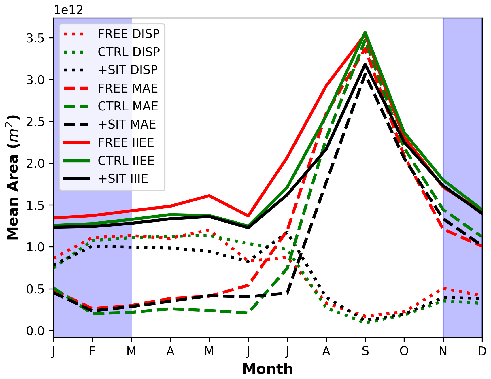
Figure 7 Climatology of IIEE, MAE and displacement (DISP) of three NorCPM experiments averaged over 2003–2023. The blue-shaded area shows the time when SIT observations are assimilated.

4.2 Prediction

We evaluate the prediction skill of our seasonal hindcasts for SIT, SIE, and IIEE using the metrics outlined in Sect. 3.1, and building on the reanalysis evaluation. For all quantities, we remove the linear trend that is highly predictable. The FREE experiment serves as a baseline for assessing skill driven by external forcings but shows minimal skill for detrended ACC (Kimmritz et al., 2019), so its results are not discussed here. Prediction skill and underlying mechanisms vary significantly by region (Bushuk et al., 2024). Our assessment spans both the pan-Arctic region and specific basins, following the approach of Bushuk et al. (2017). We use the same regions as defined in Bushuk et al. (2017), shown in Fig. 8. We compare the performance of CTRL and +SIT to highlight the role of SIT in improving predictability across different regions. We present the central Arctic, Beaufort Sea, Barents Sea, Bering Sea, and pan-Arctic regions, where the largest differences in SIE, SIT and IIEE skill between CTRL and +SIT are observed, but an assessment for other regions is also available in the Supplement. Even if the time span of our experiment covers an unprecedentedly long period to assess the impact of SIT on seasonal predictions, the limited sample size of 21 hindcasts per season makes it challenging to perform the significance test of the differences between the systems.

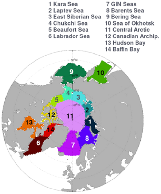
Figure 8 A map showing the regions used in this study. The regions are defined by Bushuk et al. (2017).

4.2.1 Prediction of sea ice thickness

The assimilation of SIT observations improves detrended ACC and detrended bfRMSE of SIT prediction (Figs. 9 and 10). In each region, ACCs of +SIT are positive and higher than the ones of CTRL, which are mostly not statistically significant (the top row of Fig. 9). However, in most cases, ACC of +SIT does not pass the student's t test due to the small sample size (the bottom row of Fig. 9). Results are clearer with bfRMSE. +SIT shows lower bfRMSE than CTRL in almost all four regions and target months (Fig. 10).

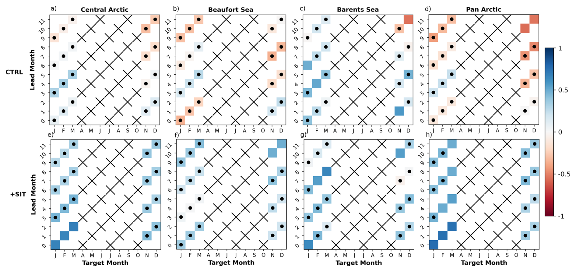
Figure 9 Detrended ACCs of our seasonal hindcasts for SIT from CTRL and +SIT with observations of SIT from CS2SMOS. Crosses are shown when comparison with observations is not possible due to lack of observations. The dots represent the ACC values that are not statistically significant.

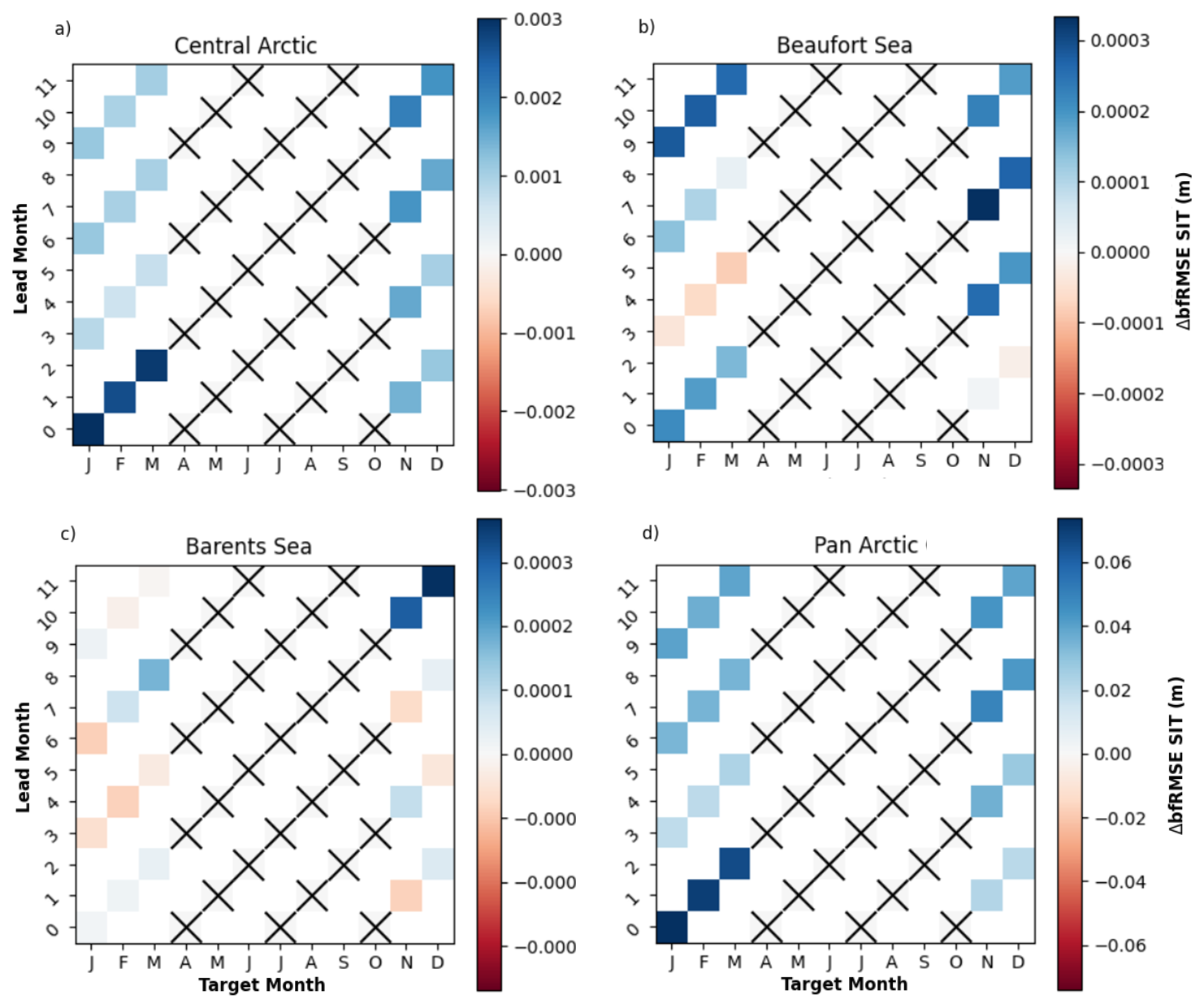
Figure 10 Differences in detrended bfRMSE of SIT from CTRL and +SIT experiments against observations from CS2SMOS. As Fig. 9, we show bfRMSE only in four of the regions defined by Bushuk et al. (2017). Blue (red) colour indicates +SIT is better (worse) than CTRL. Crosses are shown when comparison with observations is not possible due to lack of observations.

In the central Arctic, there is an overall improvement of detrended ACCs and bfRMSE for all lead months, but significant detrended ACCs +SIT are only found for +SIT in January–March. This coincides with times when detrended bfRMSE is also most reduced from CTRL. There is also a small reduction of detrended bfRMSE in winter. This suggests that the year-to-year anomaly of SIT can be predicted beyond 12 lead months.

In the Beaufort Sea, there is again an overall increase in detrended ACC (as for the central Arctic), but it is only significant in November–December, for hindcast initialised in January. Detrended bfRMSE is also strongly reduced for this hindcast. A clear improvement is also found in January–March for long lead times. It is somewhat surprising to see a degradation, in January for hindcasts started in October (at lead month 3), but an improvement for hindcasts started in March (at lead month 9). Both hindcasts assimilated the last SIT in March, but the October hindcast assimilated SIC and ocean observation from April to September in addition. This implies that the SIC assimilation degraded the accuracy of the SIT. Hence, we have seen in Sect. 4.1, that CTRL reduces error compared to FREE, but still performs substantially poorer than SIT+ for SIT. This indicates that the persistence of SIT initialisation across summer is more accurate than using SIC for updating SIT.

The benefit is much less clear in the Barents Sea. For the July-initialised prediction, there was significant ACC up to lead month 8 in February–March. There is also a significant correlation associated with a strong reduction of bfRMSE at lead month 12 in December. This is associated with a good climatology for SIT, SIE and (possibly) SID in November, December and January.

The pan-Arctic is the region for which we see the largest benefit from initialising SIT. The detrended ACC values are improved and the correlations are significant in January–March up to lead months 12. The associated detrended bfRMSE values are in agreement and also strongly reduced. Improvements in November–December are comparatively smaller than that of the later winter months, which can again be attributed to the lack of SIT observations in summer.

Overall, the SIT prediction results are quite promising and consistent with some previous studies (Blanchard-Wrigglesworth et al., 2011b, a). The impact is largest in the central Arctic and Beaufort Sea, where the observations are most accurate and where SIT anomalies persist longest. Our analysis did not assess prediction skills beyond 12 months lead time, but significant prediction skills of SIT were found to reach this limit – e.g. in the Beaufort and the Pan-Arctic.

4.2.2 Prediction of sea ice extent and sea ice edge

For the predictions of SIE, we focus on bfRMSE and IIEE, as results from the ACC are less clear. ACC differences for detecting benefits from initialization can be problematic if the skill from the externally forced climate trend is high and the ACC differences are small – the normalisation step can yield misleading results (Smith et al., 2019).

The differences in bfRMSE between CTRL and +SIT are more nuanced than for SIT, as shown in Fig. 11 and somewhat disappointing. In the central Arctic, there is little change except in the September SIE prediction for the April and July initialisations, which shows some improvements in +SIT. In the Barents Sea, the results mixed, with some improvements in predictions from January, but degradation in the other start months. In the Beaufort Sea, there are quite strong improvements around August–October for every lead time, but it does also appear to lead to some degradations in the months preceding. Finally, in the Bering Sea, improvements are more homogeneous for the first few months, with January initialised hindcast showing more substantial improvements. There are some improvements in bfRMSE in some other Pacific-side marginal regions.

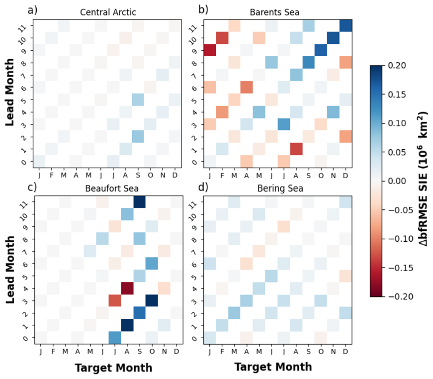
Figure 11 Difference in SIE detrended bfRMSE of CTRL and +SIT predictions computed with observations of SIE from NOAA in four Arctic regions. Blue (red) indicates that +SIT has lower (higher) bfRMSE than CTRL.

As we did for the reanalysis, we investigate the IIEE of the hindcasts in Fig. 12. The IIEE shows substantial improvement centered around September for all lead months, with improvement generally occurring between August to November. The result for the full RMSE of SIE looks very similar (not shown). As such, the location of the ice edge is improved primarily due to the bias changes in SIT, which improved the SIE bias during that period (Fig. 5). In order to better exemplify that we will look in more detail at the Beaufort Sea has consistently shown the most positive results for predictions of SIE in our study so far.

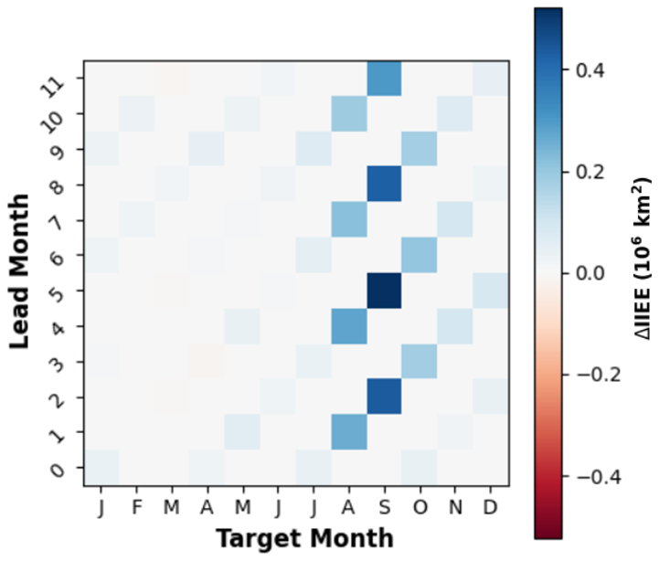
Figure 12 Difference of IIEE between CTRL and +SIT over the whole Arctic. Blue (red) means +SIT is better (worse) than CTRL.

We look at the SIE climatological mean of the hindcast in the different systems and for different start months in the Beaufort Sea (Fig. 13). The +SIT system climatological minimum is in better agreement with the NOAA observations for each start month than the CTRL and FREE predictions. The improvements are largest during the melt season – even for the October initialised hindcast. This is in good agreement with the improvements we saw for the IIEE and confirms that the main reason for improvements in IIEE relates to improving the SIT bias that reduces the bias in SIE during the melting season.

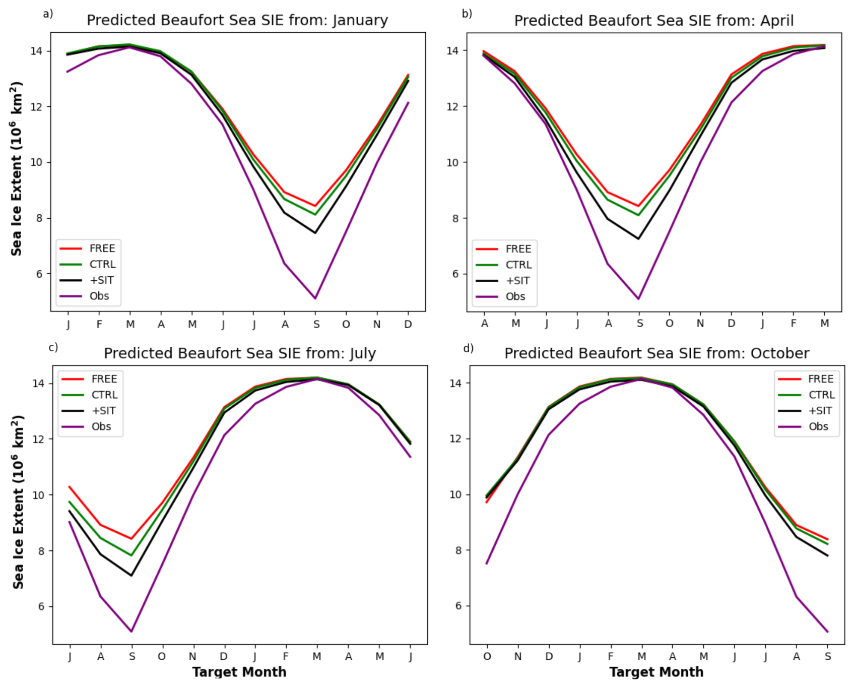
Figure 13 Climatological mean of SIE predictions from our NorCPM experiments and observations from NOAA in the Beaufort Sea. The region is as defined by Bushuk et al. (2017).

5 Discussions and conclusions

In this study, we have used the NorCPM coupled global climate model to assimilate SIT data alongside SIC, SST and ocean profiles of temperature and salinity data. We compared the performance of our system that assimilated SIT in addition to the other datasets, to highlight the role of SIT in improving predictability across different regions. We first produced a reanalysis and then used this reanalysis to initialise seasonal hindcasts (+SIT). We validated our results not only using the standard metrics (bias, bfRMSE and ACC), but also IIEE, which provides unique insights on skill at the ice edge. We also measured our results against independent SIT measurements from the BGEP ULS moorings.

We evaluated the assimilation of ENVISAT and CS2SMOS SIT data into NorCPM. While ENVISAT has higher uncertainties than CS2SMOS, it extended the reanalysis period and improved SIT and ice edge hindcast estimates in the central Arctic, particularly during the melt season through the SIT bias reduction in winter.

CS2SMOS provided more accurate data and greater reductions in biases in comparison to ENVISAT. Despite its limitations, ENVISAT data proved useful for reanalyses – highlighted by the DFS metrics that quantify the influence of each observational product – and provides meaningful observations in a period and location where observations are crucially lacking. We experienced some challenges in the transition period between ENVISAT and CS2SMOS, noticeable by discontinuities in the time series of SIE and SIV. It is because ENVISAT has a high uncertainty due to the instrumentation, which disproportionately observes thicker ice (Louet and Bruzzi, 1999; Schwegmann et al., 2016; Tilling et al., 2018). There has been some initiatives to harmonize the two products by correcting for the bias in ENVISAT using CS2 and the period where the two products observational period overlapped between 2010–2012 (Tilling et al., 2019). Using a bias-corrected ENVISAT together with CS2 could lead to further improvements in reanalysis and prediction for SIT and SIE. There will also be a possibility in the future to assimilate a recently developed ice thickness dataset dating back to 1994 (Bocquet et al., 2024), substantially lengthening the reanalysis by a further ten years and ensuring the consistency of the different sources of observations.

Our newest reanalysis +SIT showed substantial improvements compared to previous NorCPM versions (i.e., CTRL and FREE) with regard to ice thickness and ice volume. Bias and bfRMSE in SIT were both significantly reduced in +SIT, as our FREE and CTRL reanalyses have too thick ice all over the central Arctic and then large positive thickness biases in some places of up to 5 metres in comparison to CS2SMOS. The positive effects of the thickness assimilation in the +SIT reanalysis thus led to improvements in the ice volume estimates. The improvements in the volume estimates are difficult to completely validate due to the lack of sea ice volume observations, but compared well with the PIOMAS reanalysis, which has been extensively validated with thickness measurements over a long period (Schweiger et al., 2011). The +SIT reanalysis also showed a reduced bfRMSE of SIV, highlighting that the assimilation does correct more than just the SIT bias. Validation with independent BGEP ULS measurements of SIT showed that the +SIT reanalysis had substantially smaller bias and bfRMSE than CTRL and FREE, including during the ENVISAT period from 2003 to October 2010. The improvement in SIT also yielded improvement in SIE during the melting season and, therefore, also for IIEE.

We found that thickness prediction was substantially improved by the ice thickness assimilation across almost all regions. The largest part of the error reduction was from correcting model bias, which persisted throughout the year in good agreement with previous studies (Bushuk et al., 2017; Schröder et al., 2019). However, our results also showed that the SIT assimilation improved the detrended bfRMSE up to 12 lead months, with the most notable improvement in the Pan-Arctic, Beaufort Sea and the central Arctic. Skill was not as clear in the Barents Sea. The results showed that we could predict SIT anomalies for at least up to a year in some regions. It would be interesting to extend the length of the hindcast to asses up to which time scale year-to-year anomalies of SIT are predictable. We could also clearly identify the detrimental impact of the lack of SIT observations during summer, highlighting the need to consider a product that extrapolates SIT estimate during that season – as for example Landy et al. (2022).

Correcting the SIT bias and anomaly had a lower-than-expected impact on the Arctic SIE predictions. Correcting the SIT bias yielded improvements in the climatology of SIE in the melting season and, as a consequence for the IIEE metric. This improvement in late summer agreed with previous sea ice prediction studies with thickness initialisation (Bushuk et al., 2017; Schröder et al., 2019), which have found SIT assimilation can help to reduce thickness biases and thus improve SIE prediction. The reason is that SIT reduced the positive bias in our model and, as a consequence, increased the area and the transition pace towards a sea ice minimum. However, if one removes the trend and the mean bias, the SIT brings some but little added value. Some skills were identified in the Beaufort Sea during summer, central Arctic and Bering Sea. This was when and where NorCPM (CTRL) tends to perform the poorest compared to other dynamical models submitted to SIPN (Bushuk et al., 2024). Still, SIT assimilation also yielded some degradation in the other basins (e.g., Barents Sea). This was likely related to the discontinuity in the observation period (summer observations missing and transition from ENVISAT to CS2SMOS). Furthermore, it should be remembered that even if our study covers an unprecedentedly long period (21 years), this is still too short to assess robustly year-to-year variability, especially considering the large trend in Arctic sea ice that can module internal variability.

Overall, this study advances the prediction capabilities of sea ice in NorCPM through additionally assimilating SIT data alongside SST, ocean profiles of salinity and temperature and SIC data. Here, we showed some improvements in SIT, SIE and IIEE prediction using SIT initialisation. While the improvement of SIT was extended for the whole year and all lead time, SIE and IIEE were improved primarily during summer and in the central Arctic, where the improvement relates to a reduction of bias. We also found that the ENVISAT dataset can be useful for sea ice reanalyses and prediction (for monthly averages), which, to our knowledge, have been assimilated into a global climate model for the first time. Still, the SIT improvement on detrended SIE anomalies is lower than expected. As SIT plays an important role in the dynamics and thermodynamics of sea ice, a possible reason may be that the sea ice model parameters used in this study have been calibrated to compensate for model bias. This can be bias in SIT, but also bias in the other components. A new ensemble-based parameter estimate was developed in NorCPM to tune model parameters efficiently (Singh et al., 2022, 2025). For our next steps, we aim to test the use of sea ice drift assimilation for refining three key sea ice parameters: air-ice stress, ocean-ice stress, and ice strength in a version of the model state that is sustained to a low level.