
the Creative Commons Attribution 4.0 License.
the Creative Commons Attribution 4.0 License.
 | 13 Oct 2026
Subseasonal forecast improvements from sea ice concentration data assimilation in the Antarctic

Mitchell Bushuk
Michael Winton
William Gregory
Bill Hurlin
Liwei Jia
Feiyu Lu
This study evaluates the impact of sea ice concentration (SIC) data assimilation (DA) on subseasonal forecasts of Antarctic sea ice by comparing reforecast (aka, hindcast) experiment suites initialized with and without SIC DA. The two initial conditions (ICs) are evaluated against NSIDC SIC observations from 1992 to 2017. Assimilating SIC reduces mean biases and root-mean-square-errors (RMSE) and enhances anomaly correlation coefficients (ACC) of SIC. The improvement in sea ice ICs is greater in the Antarctic than in the Arctic. After SIC DA, the sea ice thickness (SIT) field becomes mostly thinner except in the interior Weddell and Ross sectors. Results from reforecast experiments show that SIC DA improves the subseasonal forecast skill of Antarctic SIC, as indicated by enhanced detrended ACC, in nearly all initialization months except December and January, when the initial improvement is quickly overtaken by a bias likely linked to the thin SIT bias. SIC DA also improves the probabilistic prediction of the sea ice edge position, as measured by the Spatial Probability Score (SPS) at subseasonal time scales. The forecast skill improvement is largest in spring, followed by winter and summer, and shows minor differences in autumn. Consistent with the IC improvement, the reforecast skill gain associated with SIC DA is more pronounced in the Antarctic than the Arctic. Our study demonstrates the critical role of SIC DA in improving subseasonal prediction of Antarctic sea ice.
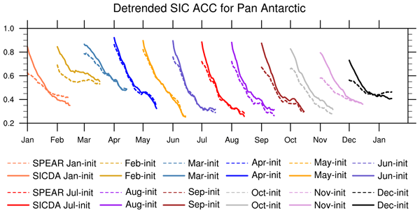
- Article
(15416 KB) - Full-text XML
-
Supplement
(20871 KB) - BibTeX
- EndNote


The Antarctic sea ice extent (SIE) experienced an overall increasing trend from the late 1970s to 2015 (e.g., Zwally et al., 2002; Cavalieri and Parkinson, 2008; Parkinson and Cavalieri, 2012; Turner et al., 2015; Zhang et al., 2019), as opposed to the continuously declining Arctic SIE. In the austral spring of 2016, the Antarctic sea ice started retreating at an unprecedented rate that led to the lowest summer SIE record in 2017 in the satellite era (e.g., Stuecker et al., 2017; Turner et al., 2017; Schlosser et al., 2018; Zhang et al., 2022a). The Antarctic SIE remained abnormally low until the present and reached record minimum lows in February 2022 (e.g., Raphael and Handcock, 2022), and then again in February 2023 (e.g., Purich and Doddridge, 2023). While Antarctic sea ice had not received as much attention as its Northern-Hemisphere counterpart, its shift from the steadily increasing trend to the recent decline stimulated a growing research community (e.g., Massonnet et al., 2023). In the meantime, human activities, including commercial shipping, fishing, and tourism, have been accelerating in recent decades. Hence, providing more accurate subseasonal predictions of Antarctic sea ice has become pressing to better manage fast-growing human activities.
The value of initialization in Antarctic sea ice predictability has been assessed by previous studies using a perfect model approach, which assumes that the models and initializations are bias free. Holland et al. (2013) show that the initial value of ocean and ice states in January provides predictability of the sea ice edge for up to 3 months and then re-emerges in the ice growth season due to the memory of heat content anomalies stored in the upper ocean. Zunz et al. (2015) explore the impact of three different data assimilation approaches to constraining sea ice and ocean initial conditions on Antarctic sea ice predictions at interannual to decadal time scales initialized from January. They find the benefit of the initialization shown in the high prognostic potential predictability and correlation with observations in the first two months, which disappears and re-emerges in the later season, attributed to the memory stored in the upper ocean heat content. They also demonstrate that the benefit of initialization may even exist in decadal time scales likely due to the interaction between sea ice and ocean heat content. Marchi et al. (2019) further employs six general circulation models (GCMs) and conducts ensemble experiments on multiple start dates to study the initial-value predictability of Antarctic sea ice. They confirm that even though they initialized the models from a different month, July, this initial skill drop in the first couple of months and skill re-emergence linked to the upper ocean heat anomalies in the subsequent winter season still exists.
The mechanisms of Antarctic sea ice predictability at seasonal to interannual time scales are similar to that of the Arctic in that the anomaly persistence of sea ice itself explains the majority of the predictability source at the lead times up to a couple of months, and the upper ocean heat anomalies contribute to predictability at the longer lead times, as shown in the above studies. While studies agree that sea ice thickness (SIT) is an important predictor for Arctic summer sea ice predictions (e.g., Blanchard-Wrigglesworth et al., 2011; Tietsche et al., 2014; Guemas et al., 2016; Bushuk et al., 2021), it is less conclusive for the role of SIT in Antarctic summer sea ice predictions at seasonal time scales. While some studies (e.g., Holland et al., 2013; Ordoñez et al., 2018; Marchi et al., 2019) suggest that SIT is not an important predictor for Antarctic summer sea ice predictions, Bushuk et al. (2021) and Xiu et al. (2025) found that the SIT initial condition provides an important source for summer sea ice prediction skill in the Weddell sector, which can be well constrained by realistic atmospheric forcings.
Whether prediction systems can turn the potential predictability into actual prediction skill is even less studied. Several reforecast studies have been done to assess it in the current seasonal prediction systems. Bushuk et al. (2021) show that the GFDL seasonal prediction systems can make skillful predictions of regional SIE and sea ice edge positions at seasonal time scales. They also demonstrate that the new systems (SPEAR_LO and SPEAR_MED) have improved summer sea ice predictions over the previous system (FLOR), mainly due to the more accurate initial conditions of SIE and SIT. Payne et al. (2023) found similar results by conducting analyses on the seasonal prediction skill of Antarctic sea ice in the Canadian Seasonal to Interannual Prediction System version 2 (CanSIPSv2). They also compared the seasonal prediction skills between the two hemispheres and found that the skill difference varies with the experiment period. The detrended skill is generally better in the Antarctic than in the Arctic from 1980 to 2019, while it's the other way around when analyses are done from 1980 to 2010.
Studies have also examined the Antarctic sea ice prediction skill at subseasonal time scales. Zampieri et al. (2019) evaluated subseasonal forecasts of the sea ice edge position from the ensemble prediction systems in the S2S database from 1999 to 2010 in both hemispheres. Only one system outperforms the benchmarks (anomaly persistence and climatology forecasts) in the 5–30 d forecast range. All systems perform worse in the Antarctic than in the Arctic, likely linked to the substantial initial errors in the Antarctic. Gao et al. (2024) extended the study of Zampieri et al. (2019) in the Antarctic by updating to the most recent S2S database and including prediction systems from the Copernicus Climate Change Service (C3S) project. Similar results are shown in their study regarding the performance of the systems in Antarctic sea ice edge predictions. They further diagnosed possible causes of the sea ice edge errors in the systems and highlighted the critical role of initial conditions (ICs). Wang et al. (2023) constructed a deep learning model for Antarctic regional sea ice at sub-seasonal time scales using only daily sea ice concentration (SIC) from observations and showed that it outperformed the three major seasonal prediction systems (the Geophysical Fluid Dynamic Laboratory, GFDL, the European Center for Medium-range Weather Forecasts, and the National Center for Environmental Prediction) examined in their study, showing higher anomaly correlation coefficient (ACC) and lower mean absolute errors, and highlighting errors in the initial condition of the dynamical models.
We have previously demonstrated the value of SIC data assimilation (DA) in improving sea ice ICs in the Arctic using the sea ice DA framework of the GFDL ocean and sea ice model and the Data Assimilation Research Testbed (DART) (Zhang et al., 2021). We further examined its value in seasonal Arctic summer sea ice predictions using the GFDL seasonal prediction system (Zhang et al., 2022b). Gregory et al. (2023, 2024) also show that SIC DA reduces systematic IC biases of Antarctic sea ice in the GFDL sea ice model. Inspired by the growing body of studies on Antarctic sea ice prediction and predictability, in this study, we thoroughly evaluate the performance of an updated version of the SIC DA product generated from our sea ice DA framework in the Antarctic. We then investigate the benefits of using the SIC DA product to initialize the GFDL SPEAR system for Antarctic sea ice prediction at subseasonal timescales. We describe the data and methodology in Sect. 2, analyze and discuss results in Sect. 3, and conclude in Sect. 4.
2.1 SPEAR System
The current GFDL modeling system for seasonal to multi-decadal predictions and projections, the Seamless System for Prediction and EArth System Research (SPEAR) (Delworth et al., 2020), is applied in this study. It consists of the Modular Ocean Model version 6 (MOM6), Sea Ice Simulator version 2 (SIS2), Atmosphere Model version 4 (AM4), and Land Model version 4 (LM4). SPEAR has two initialized seasonal prediction systems: SPEAR_LO and SPEAR_MED. They differ in their horizontal resolution in the atmosphere and land models, with SPEAR_LO having 1° and SPEAR_MED having 0.5°. They share the same nominal horizontal resolution of 1° for ocean and sea ice models. SPEAR_LO and SPEAR_MED are found to have similar seasonal prediction skill for Arctic sea ice (Bushuk et al., 2022), but the latter was shown to perform better for Antarctic sea ice (Bushuk et al., 2021). Thus, we employ SPEAR_MED in this study.
Two separate DA experiments are conducted to provide ICs for the SPEAR prediction system. An ocean DA experiment performed using SPEAR_LO provides this ocean ICs. This experiment assimilates observations of sea surface temperature (SST) and ocean temperature and salinity profiles from various sources (Lu et al., 2020). An atmosphere and SST nudging run based on SPEAR_MED provides the sea ice, atmosphere, and land ICs. This experiment nudges the wind, temperature, and humidity to the NOAA/NCEP Climate Forecast System Reanalysis and SST to NOAA's Optimal Interpolation Sea Surface Temperature (OISST). The SST is nudged to OISST when the observed SIC (also from OISST) is below 30 %, and to the freezing points calculated based on the modeled salinity when the observed SIC is >30 %. Hence, the sea ice IC is implicitly constrained by SIC observations.
2.2 Sea Ice Concentration Data Assimilation Product
We assimilate passive microwave SIC observations retrieved using the NASA Team (NT) algorithm from the National Snow and Ice Data Center (NSIDC) version 1.1 into the SPEAR MOM6/SIS2 global ice-ocean model forced by the Japanese 55-year Reanalysis (JRA55-do) (Tsujino et al., 2018), through the linked DART (Anderson et al., 2009) and SIS2. An Ensemble Adjustment Kalman Filter (Anderson, 2001) with a horizontal localization radius of approximately 170 km was used in this study. The SIC of each category (5 thickness categories in total) is the only state variable that's directly updated by DA. The ice and snow thickness of each category remain unchanged, while their aggregate thicknesses are adjusted by the update in the concentration of all categories. More technical details of the assimilation system are documented in Zhang et al. (2021). This SIC data assimilation product has been validated in the Arctic (Zhang et al., 2021) and shown to improve subseasonal-to-seasonal predictions of Arctic summer sea ice in a subsequent study (Zhang et al., 2022b).
2.3 Reforecast Experiments
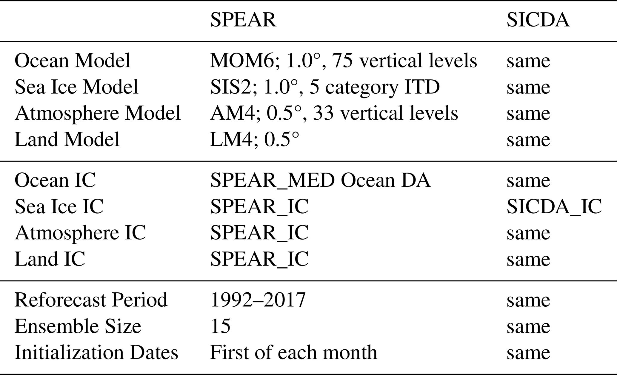
In this section, we describe the two seasonal reforecast experiment suites analyzed in this study (Table 1). Since the SPEAR_MED system has been shown to have better prediction skill for Antarctic sea ice (Bushuk et al., 2021), we employ the SPEAR_MED instead of SPEAR_LO. Our baseline reforecast suite is the standard SPEAR_MED forecast described in Sect. 2.1. Hereafter, we refer to SPEAR_MED as SPEAR for simplicity. The other reforecast experiment, SICDA, is initialized from the SIC DA product described in Sect. 2.2. SICDA has the same initial conditions for the ocean, atmosphere, and land as SPEAR. We refer to their ICs as SPEAR_IC and SICDA_IC, respectively. Each reforecast experiment consists of 15 ensemble members, covering the period 1992–2017. The reforecasts are initialized on the first day of each month and integrated for one year. Only the first 45 d are analyzed in this study as we focus on the subseasonal time scale of their prediction skills.
2.4 Reference Forecasts
We use the damped anomaly persistence forecast (damped persistence hereafter) as the baseline reference forecast. The damped persistence forecast is calculated using the NSIDC NT SIC observations for each grid cell and consists of two components: a linear trend climatology and a scaled anomaly. For a given grid cell on a given target date, we calculate the slope and intercept using the observed SIC on this day in all the past years (e.g., 1979 to the year before the target year) to compute the linear trend climatology. The scaled anomaly is computed by multiplying the observed anomaly on the day before the initialization date by a scaling factor. The scaling factor considers the lagged correlation between the observed SIC on the initialization date and the target date. The detailed equation can be found in Eq. (5) in Bushuk et al. (2024).
2.5 Observation and Reference Data
The NSIDC SIC observations derived using the NT algorithm are used in this study. The NSIDC NT SIC observations are assimilated into the SICDA_IC and are also used to evaluate the results of the reforecast experiments.
We also consider SIT analysis data from the Global Ice-Ocean Modeling and Assimilation System (GIOMAS; Zhang and Rothrock, 2003) as a reference data set. The GIOMAS SIT data is not an observation data set, nor has it assimilated any SIT observation data. Previous studies (e.g., Liao et al., 2022; Shi et al., 2021) evaluated it against satellite retrievals, shipping and airborne observations and concluded that the GIOMAS SIT field can reasonably represent the interannual variability, and trends of Antarctic sea ice, although it suffers from biases. It was found to underestimate SIT, especially in the deformed ice zone, for example, the northwestern Weddell sector. Note that the GIOMAS SIT data set is not used for model validation in this study, but rather a reference, as has been used in other Antarctic sea ice studies (e.g., Shu et al., 2015; DuVivier et al., 2020; Selivanova et al., 2024).
Another SIT reference dataset we use is from the Southern Ocean State Estimate (SOSE) that comes from the Southern Ocean Carbon and Climate Observations and Modeling (SOCCOM) project (Mazloff et al., 2010). The most recent endeavor includes a biogeochemical component (BSOSE), which assimilates all the available physical and biogeochemical ocean observations from floats, ships, and satellites in the Southern Ocean into the MIT general circulation model (Verdy and Mazloff, 2017). Although BSOSE does not assimilate any SIT observations, we select it alongside with GIOMAS because its higher regional resolution, dynamically consistent ocean circulation fields, and constraints from ocean profiles, SST, and SIC observations should provide a complementary SIT reference that GIOMAS, with its global coverage and coarser resolution, cannot offer. The monthly SIT data from the 105th iteration of the BSOSE dataset is used in our study. Note that both datasets provide the ice thickness per grid cell, which is referred to as sea ice volume (SIV) in convention.
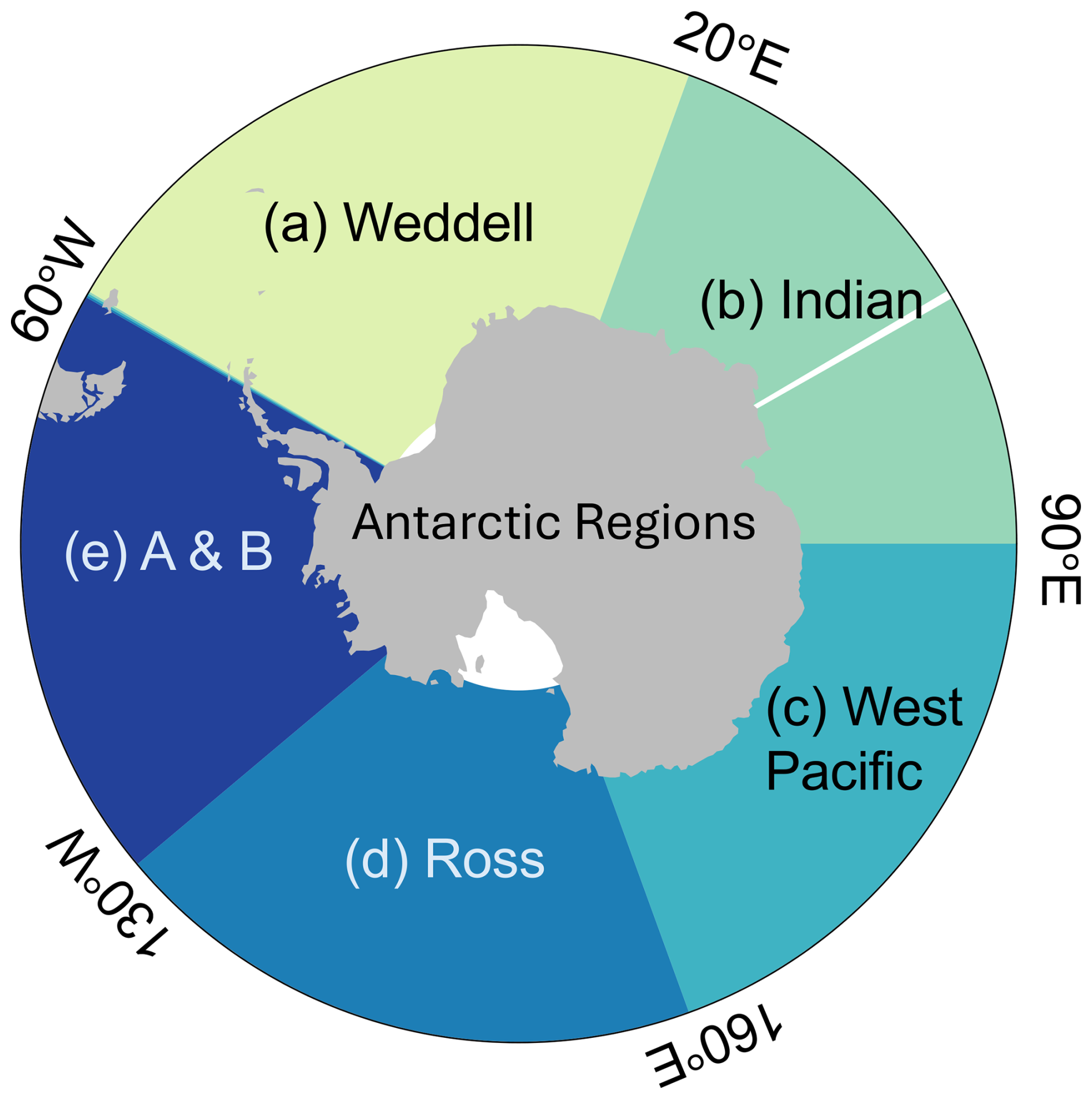
Figure 1The Antarctic regions defined in this study. The longitude boundaries of the regions are: (a) 60° W–20° E for Weddell, (b) 20–90° E for Indian, (c) 90–160° E for West Pacific, (d) 160° E to 130° W for Ross, and (e) 130–60° W for Amundsen and Bellingshausen (A and B hereafter).
2.6 Skill Metrics
We evaluate the regional SIE and grid-cell level SIC from the two ICs. The regional SIE is the sum of the area where SIC is greater than 15 %. The Antarctic ocean is divided into five sectors following the convention in Bushuk et al. (2021); see also our Fig. 1. We evaluate the two model ICs using the detrended anomaly correlation coefficient (ACC), bias, and Root-Mean-Square Error (RMSE). We first take the ensemble mean of SIC from the 30 members of each initial condition data set. We then calculate the skill metrics using the ensemble mean. We use the detrended ACC and RMSE to evaluate the reforecast skill of SPEAR and SICDA as well. The detailed equations are documented in the Sect. 2d in Zhang et al. (2022b). When we look at the skill of grid-cell level SIC averaged for sub-regions, we only average skills within the ice variability zone. We define the ice variability zone as the grid cells where the observed interannual variability is larger than 10 %.
In addition, we calculate the Spatial Probability Score (SPS; Goessling and Jung, 2018) to evaluate the sea ice edge predictions of SPEAR and SICDA. We define SPS as
where Pf(i) and Po(i) are the sea ice probabilities at the grid cell i. Pf is the percentage of ensemble members with larger than 15 % SIC for the SPEAR ensemble forecast and either 0 (SIC <15 %) or 1 (SIC >15 %) for the deterministic damped persistence forecast. Po is also 0 or 1 since observations are deterministic as well. S is the integral surface area evaluated over a spatial domain (Arctic or Antarctic ocean). Since the Arctic and Antarctic have different ranges of sea ice variability, directly comparing the SPS values in the two hemispheres is unfair. We thus normalize the SPS values by dividing them by the SPS of a trend climatology forecast for each hemisphere. The normalized SPS is referred to as nSPS.
We apply a bootstrap resampling method (with 1000 iterations) to determine whether the reforecast skills of two experiments differ significantly. For ACC of SIC, at each grid cell and iteration, we resample with replacement from the time series of each experiment and the corresponding observations, and compute the skill metric for both. We then calculate the area-weighted ACC for each experiment and their difference. After 1000 iterations, we consider experiment A to be significantly better than experiment B if its skill value exceeds that of experiment B in at least 950 (i.e., ≥95 %) of the bootstrap samples, and vice versa. The same procedure is applied to nSPS, with the skill metric computed across the 1000 iterations.
3.1 Sea Ice Initial Conditions
We first compare the two sea ice ICs. Section 3.1.1 evaluates SIE and SIC, and Sect. 3.1.2 compares SIV. Note that the SIC and SIE fields are evaluated against the NSIDC observations, while the SIV fields are only compared against the GIOMAS and BSOSE datasets for reference. The twelve months are grouped into 4 seasons, defined as summer (January–March), autumn (April–June), winter (July–September), and spring (October–December).
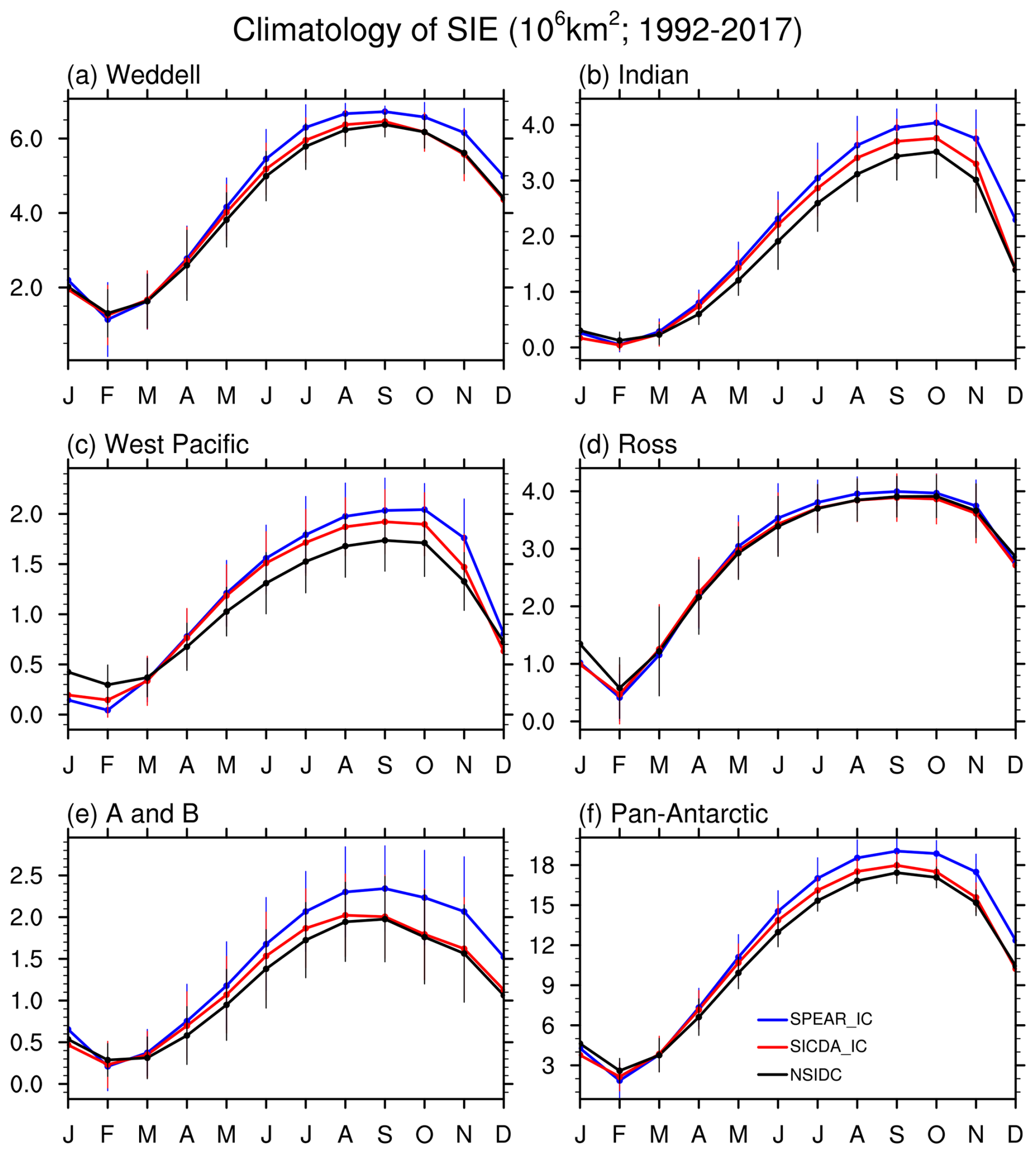
Figure 226-year (1992–2017) mean seasonal cycle of regional and pan-Antarctic SIE for SPEAR_IC (blue), SICDA_IC (red), and the NSIDC observations (black). Each error bar represents two standard deviations of regional SIE calculated over the years.
3.1.1 Sea Ice Concentration and Extent
Figure 2 shows the seasonal cycle of the regional and pan-Antarctic SIE from the two ICs and the NSIDC observations. SPEAR_IC underestimates summer SIE in general, especially in the West Pacific and Ross sectors, but it overestimates SIE in other seasons across the pan Antarctic. By assimilating SIC, SICDA_IC reduces the biases in all months. The largest bias reduction happens in the Weddell and Amundsen–Bellingshausen sectors, where most of the positive biases in winter and spring are corrected. The magnitudes of the positive biases in winter and spring SIE in the Indian and West Pacific sectors are also reduced. The positive biases in autumn are less affected in all the sectors. The summertime negative biases have not been reduced as substantially, except in the West Pacific sector. SICDA_IC also has higher detrended correlation with the observed SIE (Fig. S1 in the Supplement), showing that it simulates better interannual variability of regional Antarctic SIE.
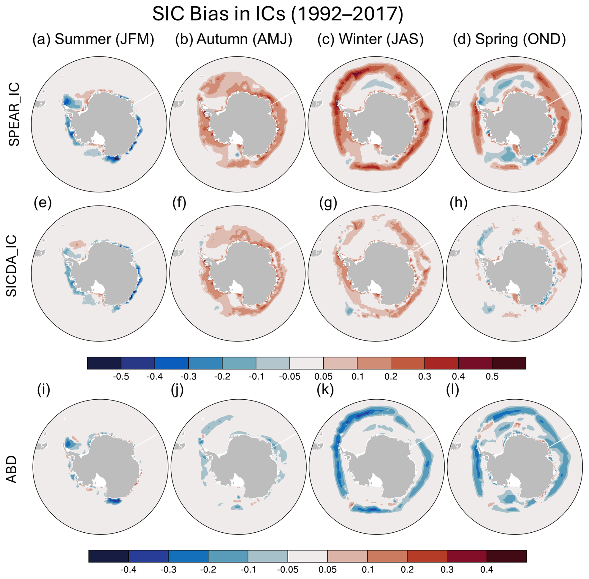
Figure 3SIC Bias for each season for SPEAR_IC (a–d), and SICDA_IC and (e–h), and their absolute bias difference (ABD; SICDA_IC – SPEAR_IC; i–l). The biases are calculated against NSIDC SIC observations from 1992–2017.
Figure 3 shows the spatial pattern of SIC biases in four seasons. SPEAR_IC has negative biases across the Antarctic Ocean in summer, except the positive bias in the East Weddell sector (Fig. 3a), which offset the negative bias in the West Weddell sector, so the biases don't show up in the Weddell SIE in Fig. 2a. The bias sign changes in autumn (Fig. 3b) when positive biases dominate the variability zone throughout the rest of the year (Fig. 3c and d), while a negative bias emerges in winter (Fig. 3c) and lasts through spring (Fig. 3d) in the interior Eastern Weddell and West Indian sectors. The Ross sector also has an expansive negative bias in spring, which cancels the positive biases elsewhere and results in a less biased regional SIE in the Ross sector as shown in Fig. 2d. The negative biases (in winter and spring in the Weddell sector and spring in the Ross sector) are located in the regions where open-water polynyas tend to happen, suggesting that the polynyas simulated in SPEAR_IC might be too active or intense. SICDA_IC decreases the magnitude of both positive and negative biases across the Antarctic (Fig. 3i–l). Notably, the wintertime and springtime positive biases in the Weddell and Ross sectors in SPEAR_IC are almost gone in SICDA_IC (Fig. 3g and h). The impact of SIC DA is much smaller in summer and autumn. In summer, SICDA_IC reduces the negative biases in the West Weddell and West Pacific sectors, and the positive bias in the East Weddell sector (Fig. 3e). In autumn, SIC DA reduces the positive biases partly, but there are still sizable positive biases around the Antarctic (Fig. 3f). There are also slight bias increases along the coastal Indian sector, part of the coastal West Pacific in summer (Fig. 3i) and spring (Fig. 3l).
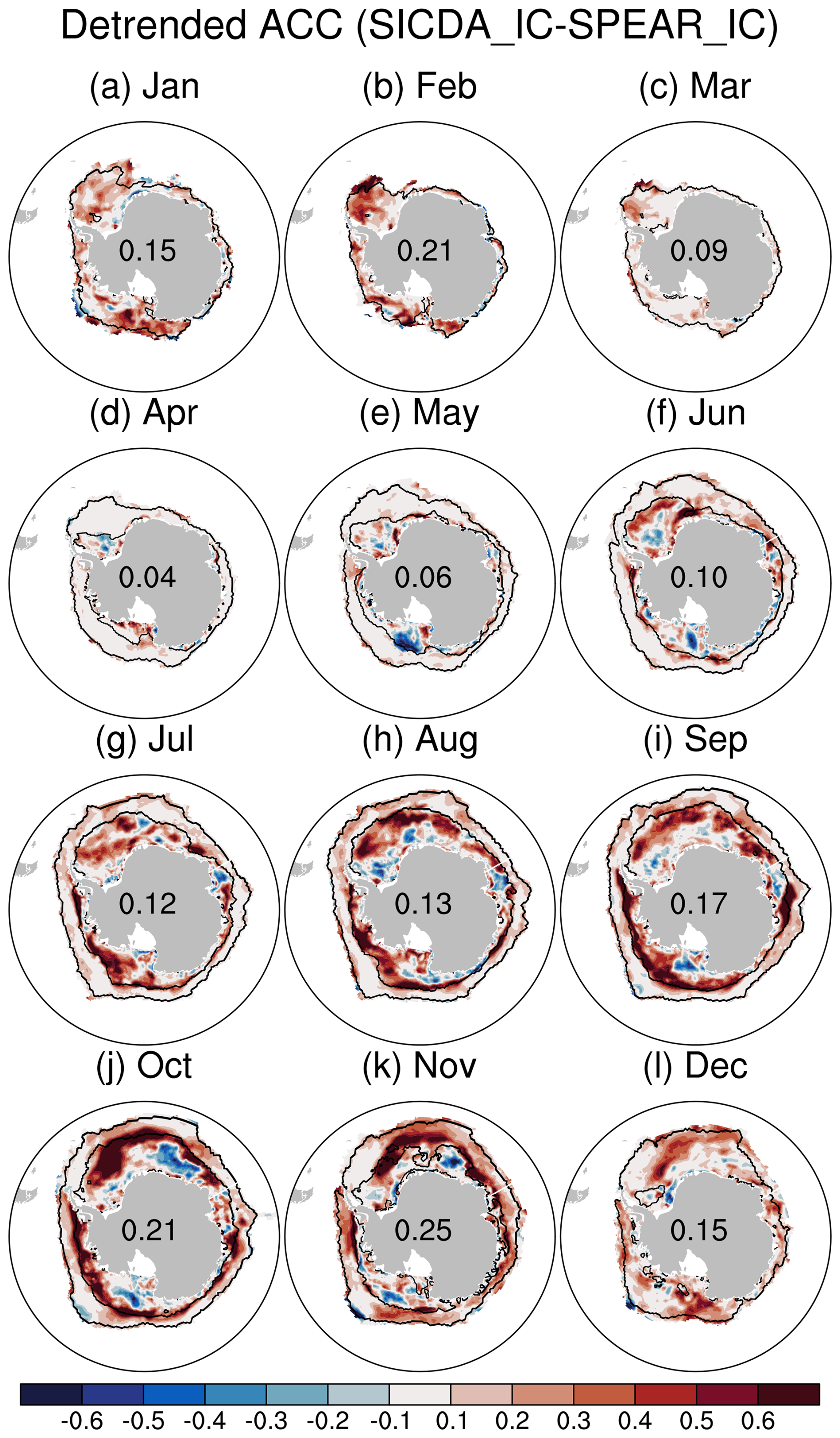
Figure 4Difference in detrended SIC Anomaly Correlation Coefficient (ACC) between the two ICs (SICDA_IC – SPEAR_IC) for each month. The black lines on each map represent the observed 10 % SIC variability zone. The numbers on each map are the area-weighted average of the detrended ACC difference within the 10 % SIC variability zone.
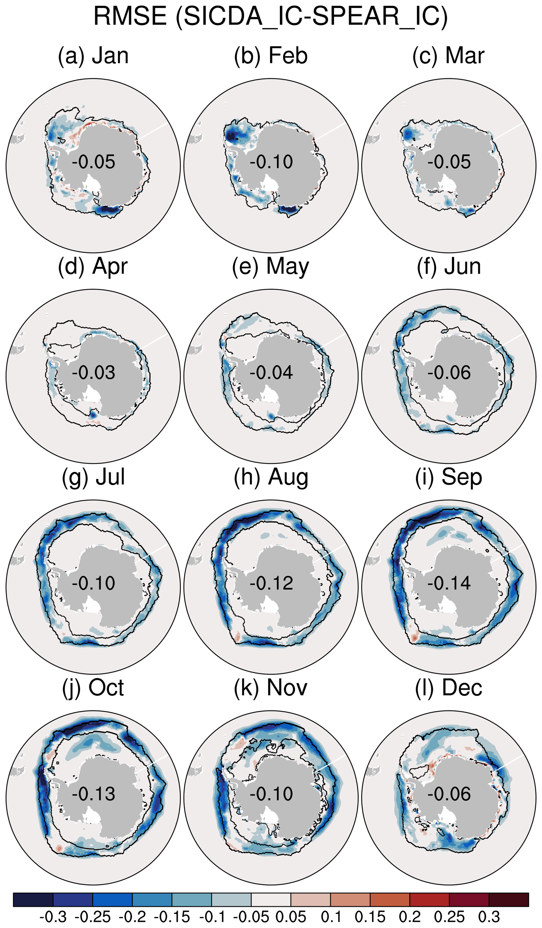
Figure 5Difference in SIC RMSE between the two ICs (SICDA_IC – SPEAR_IC) for each month. The black lines on each map represent the observed 10 % SIC variability zone. The numbers on each map are the area-weighted average of the RMSE difference within the SIC variability zone.
SICDA_IC shows predominantly better interannual variability of SIC than SPEAR_IC (Fig. 4). The largest improvements are in spring both in the variability zone and the interior ice pack, followed by additional large improvements in winter in the interior, and summer in the variability zone, and smaller improvements in autumn. SICDA_IC also reduces total error almost everywhere compared to SPEAR_IC as shown in the RMSE difference map (Fig. 5). The RMSE reduction is mostly located in the ice variability zone, while it remains less impacted in the interior. One small exception is the RMSE increase that appears along the coast of the East Weddell in January and December, and along the coast of the West Pacific in December. Compared to the Arctic, the Antarctic has a much larger ice variability zone since it's not bounded by land. SICDA_IC has, on average, a smaller ACC increase (Fig. S2) and RMSE decrease (Fig. S3) in the ice variability zone in the Arctic than in the Antarctic. The maximum improvement from SIC DA seems to happen in different seasons in the two hemispheres. While the Antarctic sea ice benefits from SIC DA mostly in spring and winter, the Arctic sea ice shows the largest improvement in summer.
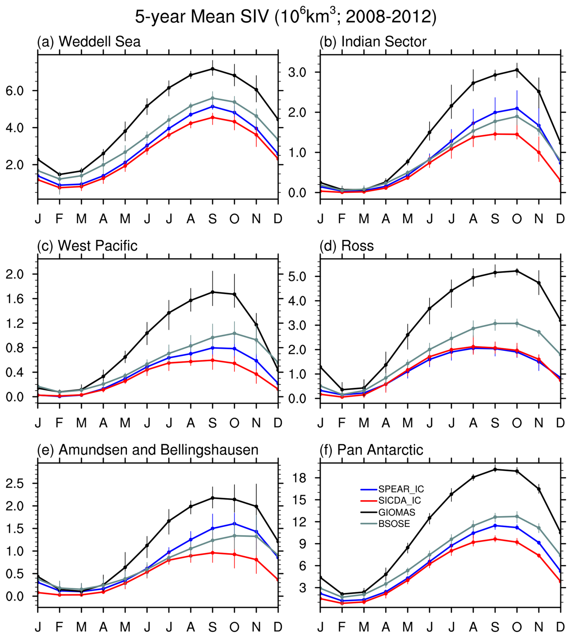
Figure 65-year mean seasonal cycle of the regional and pan-Antarctic SIV from SPEAR_IC (blue), SICDA_IC (red), GIOMAS (black), and BSOSE (gray). The values are calculated over their overlapping years, 2008–2012. Each error bar represents the range of values across the years.
3.1.2 Sea Ice Volume
We compare SIV from the two ICs and two reference datasets, GIOMAS and BSOSE. Figure 6 shows the monthly mean SIV averaged over the common period (2008–2012) of the four data sets. There are significant discrepancies among the datasets. GIOMAS has the largest mean SIV in all the regions throughout the year. SPEAR_IC, SICDA_IC, and BSOSE are closer to each other, and they mostly overlap within two standard deviations. BSOSE generally has larger mean SIV than SPEAR_IC except in the Indian and Amundsen–Bellingshausen sectors, where it has lower SIV in the winter months. SICDA_IC has the lowest mean SIV in almost all the regions in all months, with the only exception in the Ross sector where SICDA_IC is nearly the same as SPEAR_IC. This homogeneous reduction in SIV seen in SICDA_IC from SPEAR_IC is consistent with the overall decrease in SIE as shown in Fig. 2. We discussed in Zhang et al. (2021) that SIC and SIT usually change in the same direction due to SIC DA. Since our background model has a systematic positive bias in SIC/SIE, SIC DA tends to reduce SIC/SIE and, consequently, SIT/SIV. The same plot but over a longer record for GIOMAS and our ICs indicate that this feature is generic (Fig. S3).
It is also interesting to note that the four datasets do not peak in the same month in the West Pacific, Ross, and Amundsen–Bellingshausen sectors. In the West Pacific sector, GIOMAS, SPEAR_IC, and SICDA_IC peak in September, while BSOSE peaks in October. In the Ross sector, GIOMAS peaks in October, BSOSE peaks in September, and our two initial conditions peak in August. In the Amundsen–Bellingshausen sector, GIOMAS and SICDA_IC peak in September, SPEAR_IC peaks in October, and BSOSE peaks in November. For the pan-Antarctic SIV, BSOSE peaks in October, while the rest peak in September. A longer period suggests this difference in the SIV maximum month is typical in GIOMAS and the two ICs (Fig. S4).
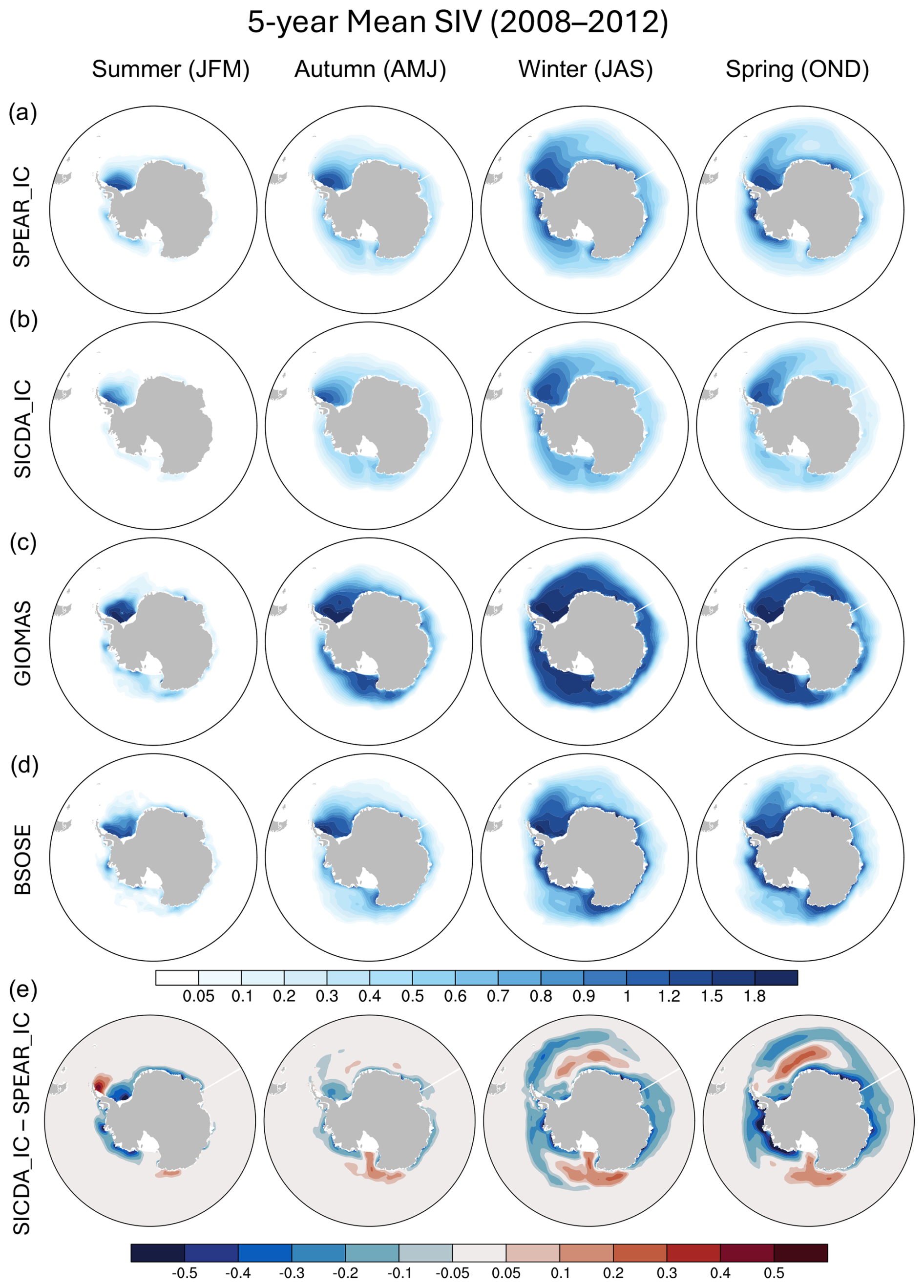
Figure 7Spatial map of the 5-year mean SIV for each season from the four data sets: (a) SPEAR_IC, (b) SICDA_IC, (c) GIOMAS, and (d) BSOSE, and (e) SICDA_IC – SPEAR_IC.
Figure 7 shows that all datasets agree that the majority of summer minimum ice is located in the West Weddell sector. In summer, while SPEAR_IC, GIOMAS, and BSOSE have some ice thicker than 0.6 m in the Ross and Amundsen–Bellingshausen sectors, SICDA_IC has no ice thicker than 0.05 m in those regions. As Fig. 6 shows, their discrepancy gets larger in the growing and peak seasons. GIOMAS has much thicker ice than the other datasets across the Antarctic Ocean (Fig. 7c). SICDA_IC has the thinnest ice overall (Fig. 7b). As sea ice grows, a thick sea ice band extending from the west to east across the Weddell sector emerges in all datasets. This band is narrower in SPEAR_IC and expands northeasterly to the Indian sector, which creates a hole in the West Indian sector in spring. This feature is not seen in the other data sets. GIOMAS and BSOSE have generally thicker sea ice along the coast than the two ICs. Figure 7e highlights the SIV difference between the two ICs. SICDA_IC is overall thinner than SPEAR_IC along the coast in all seasons, with some exceptions. SICDA_IC has thicker ice in the West Weddell in summer and in the interior Weddell and Indian sectors in winter and spring. It also has thicker ice in the Ross sector in all seasons. These are also regions where SICDA_IC reduces the negative SIC biases, e.g., the Weddell sector in winter and spring and the Ross sector in spring (Fig. 3g and h). A longer period shows similar features for GIOMAS, SPEAR_IC, and SICDA_IC (Fig. S5).
3.2 Reforecast Skill
This section evaluates the skill differences between the two reforecast experiment suites: SPEAR and SICDA. We use the damped persistence (DP) forecasts as a benchmark. We also compare the skill differences in the Antarctic to those in the Arctic to assess whether and how SIC DA influences forecast skill differently in the two poles. We use the detrended ACC and RMSE as skill metrics to evaluate the performance of their grid-cell level SIC predictions in Sect. 3.2.1, and nSPS to evaluate their probabilistic predictions of the sea ice edge position in Sect. 3.2.2. Finally, we discuss the skill degradations found in SICDA in Sect. 3.2.3.
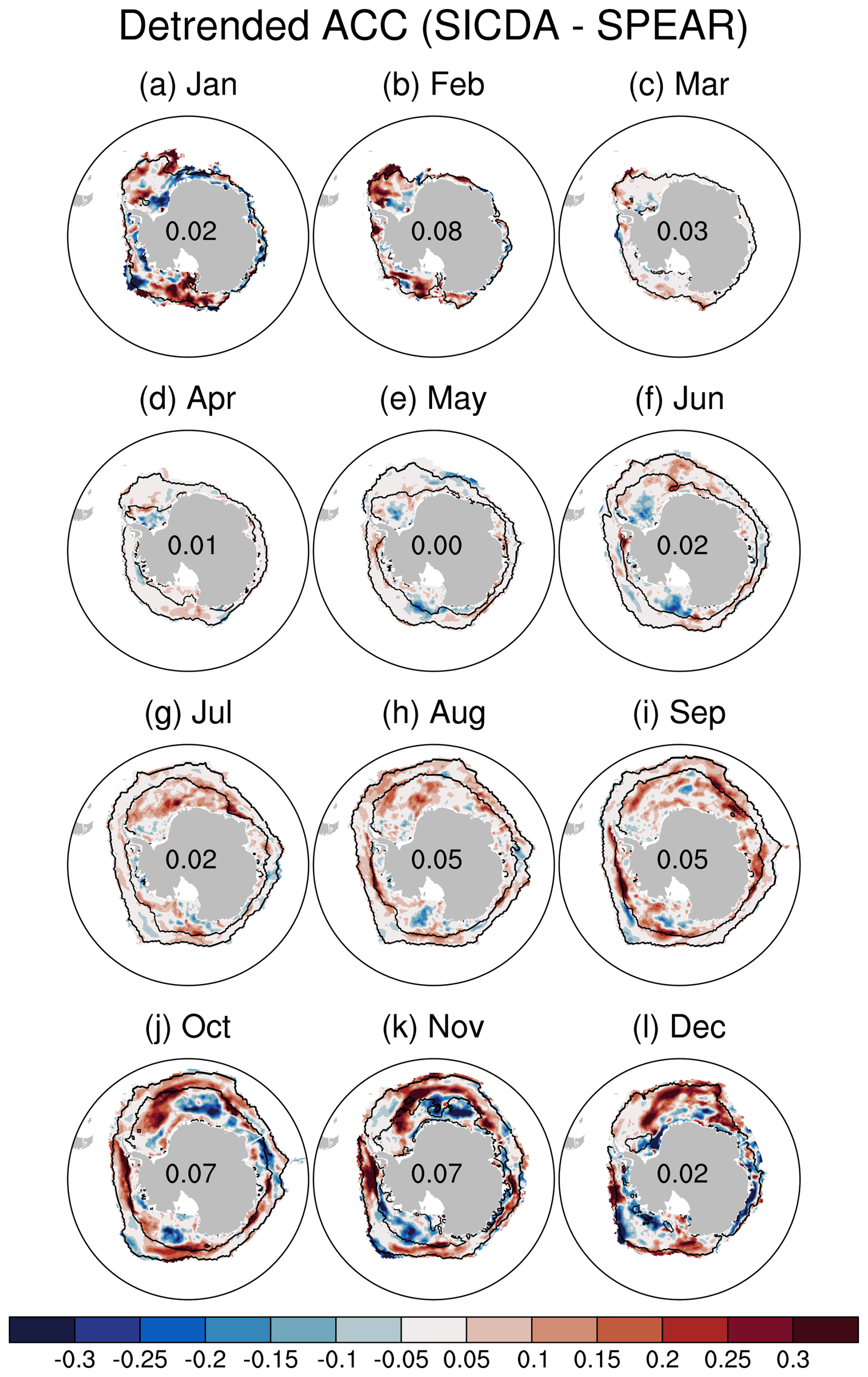
Figure 8Difference in the 45-forecast-day mean of the detrended SIC ACC between the two reforecast experiments (SICDA − SPEAR). The black lines on each map represent the observed 10 % SIC interannual variability zone. The numbers on each map are the area-weighted average of the ACC difference within the SIC variability zone.
3.2.1 Grid-cell level Sea Ice Concentration
Figure 8 shows that SICDA has increased the 45 d mean forecast skill in terms of the detrended SIC ACC for all the initialization months. The most considerable improvement is in spring (October to December). The skill improvement is also noticeable in winter (July to September) and summer (January to March) but negligible in autumn (April to June). However, in the Arctic, the SIC skill improvement is most significant in summer (July to September), moderate in spring (April to June), and minor in other seasons (Fig. S6).
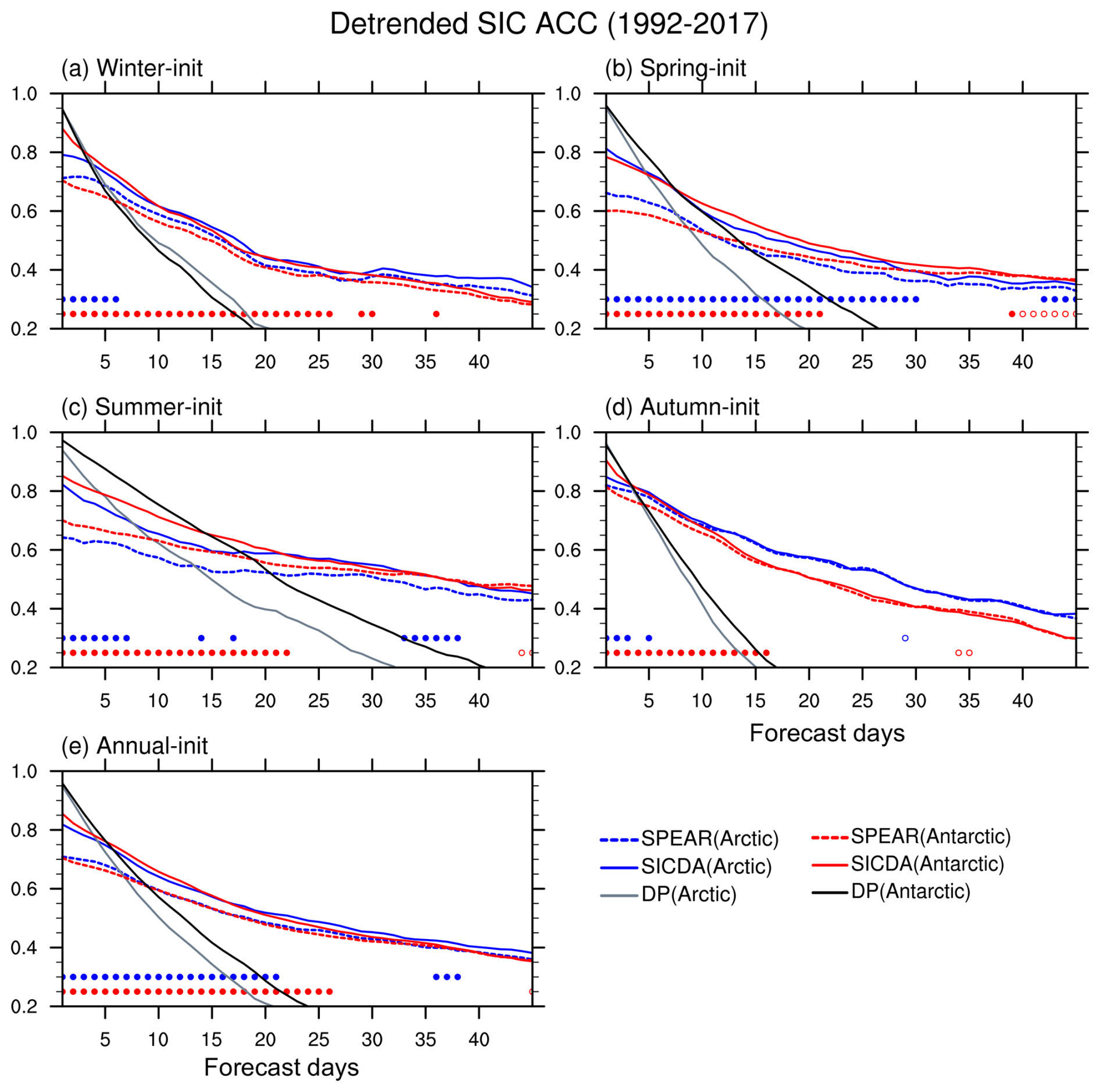
Figure 9Detrended SIC ACC averaged over the Antarctic ice variability zone as a function of forecast days for SPEAR (red dashed lines), SICDA (red solid lines), and DP (black lines), and over the Arctic ice variability zone for SPEAR (blue dashed lines), SICDA (blue solid lines), and DP (gray lines). The Detrended ACC values are calculated for each initialization month and then averaged over the (a) winter months, (b) spring months, (c) summer months, (d) autumn months, and (e) all 12 months. Each red filled circle on the bottom indicates that the detrended ACC of SICDA is significantly higher than that of SPEAR, and red open circle the detrended SIC ACC of SICDA is 95 % significantly worse than that of SPEAR for the corresponding forecast day in the Antarctic. The blue filled circles and open circles are for the Arctic, respectively.
We take an area-weighted average of the detrended ACC in the ice variability zones in both poles for each initialization season and also annual mean in Fig. 9. The DP skill decays slowest in the summer-initialized forecast in both hemispheres, followed by spring, winter, and autumn. This suggests that the SIC anomaly persists longer and thus provides more predictability in summer and spring at subseasonal time scales than in winter and autumn. Figure 9 shows that the DP forecast skill for the Antarctic sea ice is better than that for the Arctic in spring and summer, similar in winter and autumn, thereby giving an overall better skill for the Antarctic than the Arctic. It indicates that the SIC anomaly is more persistent in the Antarctic than in the Arctic at subseasonal time scales.
Both reforecast experiments lose to the DP in the beginning but are able to beat the DP within the first week annually (Fig. 9e). SICDA performs significantly better than SPEAR at short lead times in both hemispheres, and its advantage decreases gradually with forecast days. The initial skill gaps between the two reforecast experiments are more prominent in the Antarctic than in the Arctic for all seasons except summer (solid vs. dashed lines in Fig. 9). Figure 9 also shows that SPEAR is generally less skillful in the Antarctic than the Arctic in autumn and winter, suggesting a larger room for correction in the Antarctic. In contrast, SICDA shows slightly better skill in the Antarctic than in the Arctic in the first two weeks in winter and summer. This confirms that the sea ice IC is improved more in the Antarctic than in the Arctic by assimilating SIC observations.
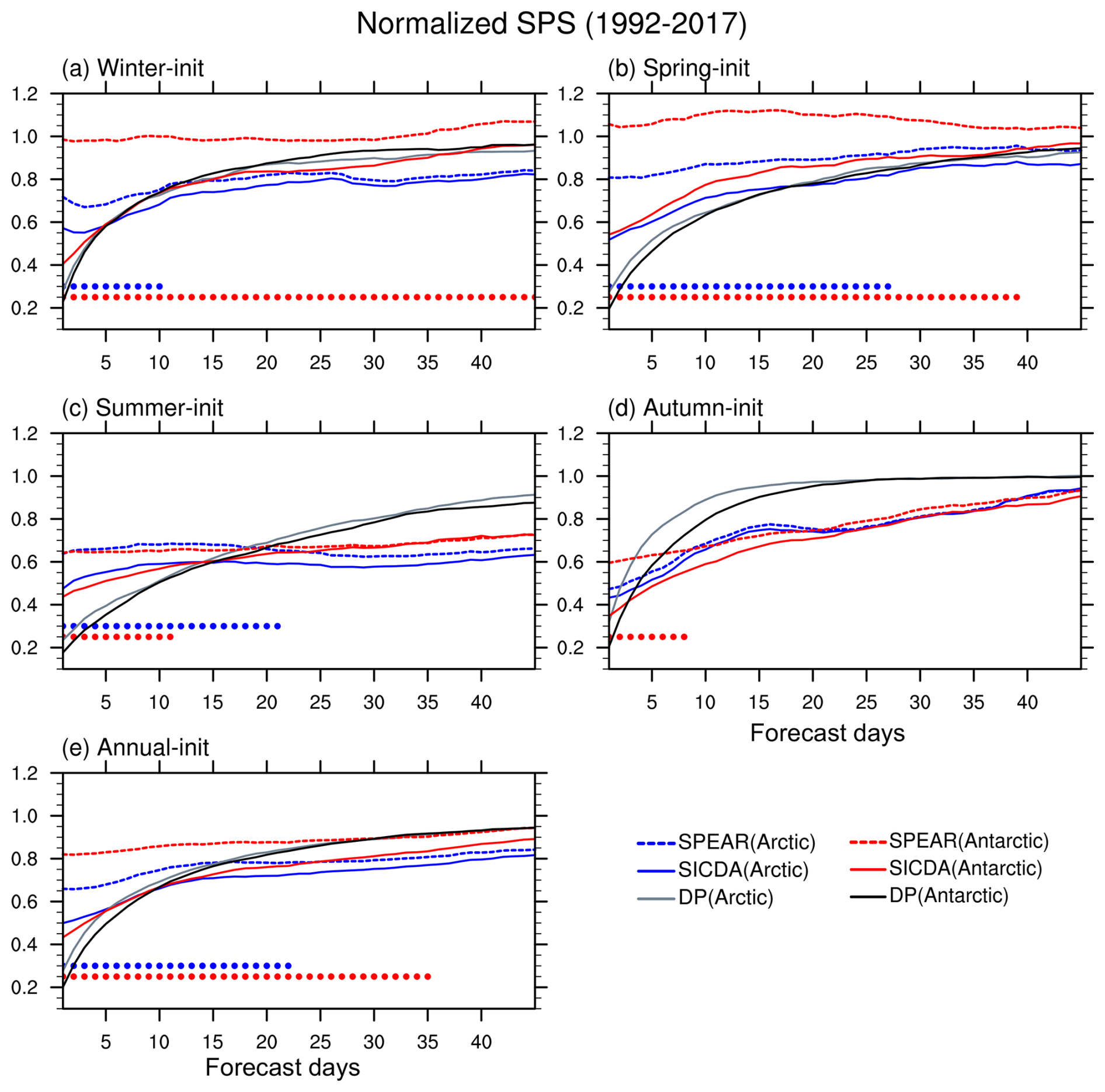
Figure 10Normalized SPS calculated over the Antarctic as a function of forecast days for SPEAR (red dashed lines), SICDA (red solid lines) and DP (black lines), and over the Arctic for SPEAR (blue dashed lines), SICDA (blue solid lines) and DP (gray lines). The SPS values are normalized by the SPS values of the trend climatology forecast for each hemisphere. The normalized SPS values are calculated for each initialization month and then averaged over the (a) winter months, (b) spring months, (c) summer months, (d) autumn months, and (e) all 12 months. Each red filled circle on the bottom indicates that the SPS value from SICDA is lower than that of SPEAR at the 95 % significant level. The blue filled circles are for the Arctic.
3.2.2 Sea Ice Edge Predictions
We use the skill metric nSPS to assess the probabilistic prediction skill of the sea ice edge from the two reforecast experiments and how they compare to the DP forecast (Fig. 10). A smaller/larger than one nSPS value indicates that the forecast is better/worse than the trend climatology. Since the DP forecast incorporates the anomaly persistence forecast in the short term and trend climatology in the longer term, its nSPS values should be smaller than one at short lead times and converge to one at longer lead times. And if a model reforecast has smaller nSPS values than the DP forecast, it's considered to have a skillful probabilistic prediction of sea ice edges. The DP forecast has slightly smaller nSPS values in the Antarctic than in the Arctic, except in winter (Fig. 10). This is consistent with its relative skill difference in the two hemispheres regarding the detrended SIC ACC discussed earlier.
SPEAR has nSPS values that are close to or higher than one in the winter and spring-initialized forecasts (Fig. 10a and b), meaning it does not have skill in winter or spring in the Antarctic. Its SPS values do not increase much with forecast days, indicating a sizeable initial sea ice edge bias in its IC. Consequently, SICDA displays the most considerable skill improvement in these two seasons. Its nSPS values are significantly lower than those of SPEAR in the entire 45 d in the winter-initialized reforecast, and for about 40 d in the spring-initialized reforecast (see red dots in Fig. 10a and b). SICDA starts to beat the DP forecast around day 15 in winter, but remains less skillful than the DP in spring. Both SPEAR and SICDA make skillful predictions of the sea ice edge for summer and autumn. SPEAR outperforms the DP at ∼ day 20 in summer and ∼ day 5 in autumn, while SICDA outperforms DP at ∼ day 15 in summer and ∼ day 2 in autumn. SICDA has significantly better skill than SPEAR for about 12 d in summer and 8 d in autumn, which is a less prominent improvement than in winter and spring. Annually, SICDA performs significantly better than SPEAR for 35 d. While SPEAR fails to beat the DP within the 45 forecast days, SICDA outperforms the DP after day 10.
In the Arctic, SPEAR shows better skill in winter and spring than in the Antarctic. It beats the DP quickly in both poles (∼2 d in the Arctic and ∼6 d in the Antarctic). It remains less skillful than the DP in spring but ties with it by the end of the 45 forecast days. SICDA consistently outperforms SPEAR; its improvement is statistically significant for 10 d in winter and 27 d in spring, which lasts shorter than in the Antarctic. It also beats the DP after ∼20 d in spring, while it always loses to the DP in the Antarctic. In summer and autumn, the nSPS values in the Arctic of SPEAR are very similar to those in the Antarctic. The skill improvement from SICDA is 95 % statistically significant for 21 d in summer and not significant at all in autumn. Annually, both reforecasts show better skill in the Arctic than in the Antarctic relative to the DP forecast. The improvement from SIC DA lasts shorter in the Arctic (22 d) than in the Antarctic (35 d).
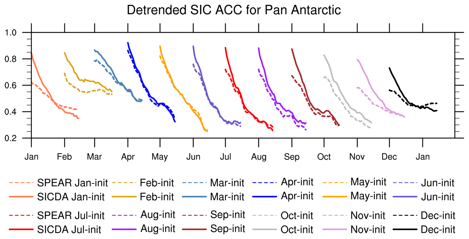
Figure 11Detrended ACC of SIC averaged over the Antarctic ice variability zone as a function of forecasting days from the 12-initializaiton months for SPEAR (dashed lines) and SICDA (solid lines).
3.2.3 Degradations
Figure 11 shows the skill evolution in terms of pan-Antarctic averaged detrended SIC ACC for each initialization month. For most months, there is an initial improvement from SICDA over SPEAR, and the skill values gradually merge. The size of the initial gap and how long it lasts vary by season. However, in the January and December-initialized reforecasts, SICDA loses to SPEAR after ∼20 forecast days. The skill degradation of SICDA relative to SPEAR is not seen in the Arctic, where SICDA consistently merges with SPEAR after an initial improvement (Fig. S7). Figure 8 indicates that the degradation happens mainly along the coast.
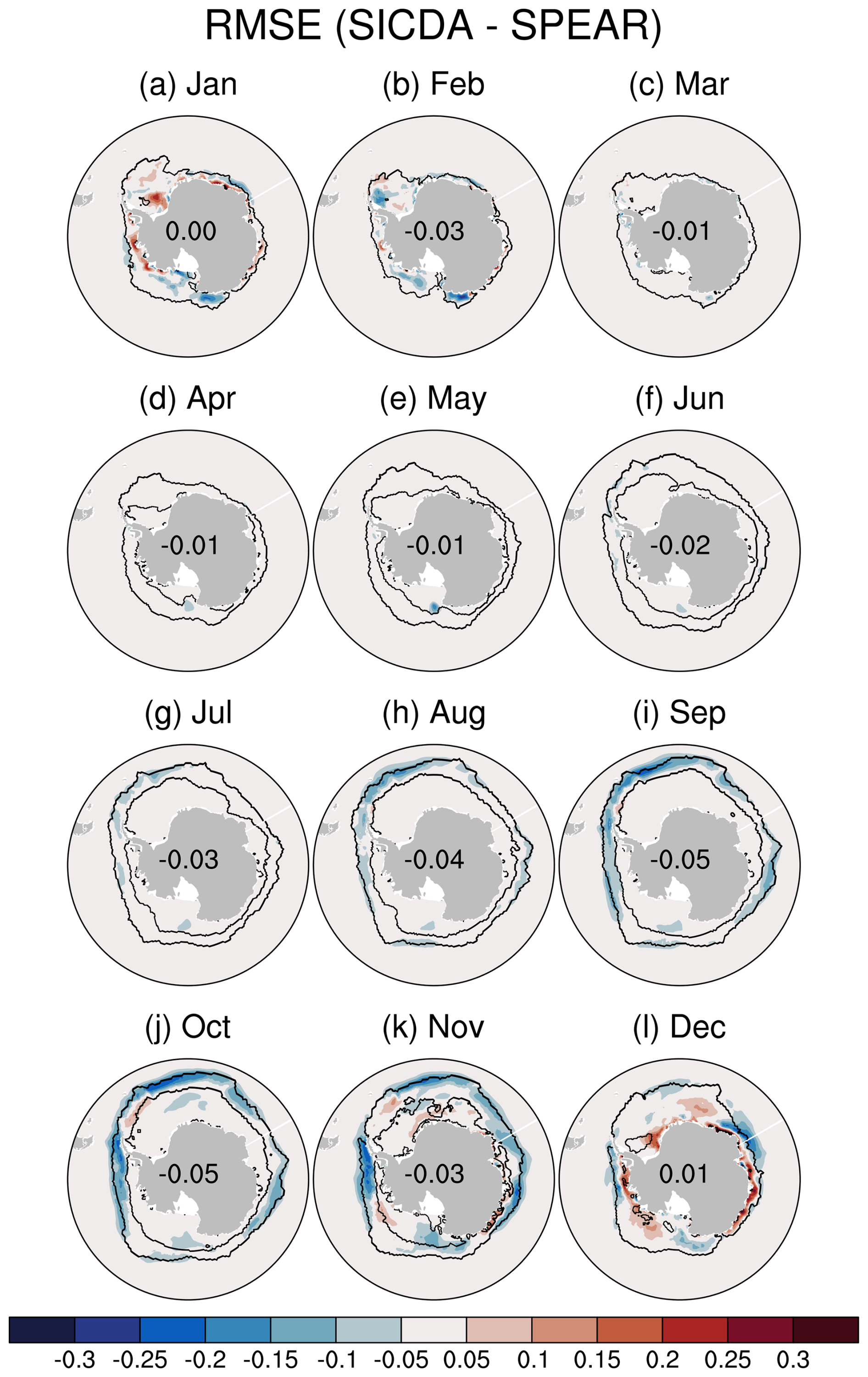
Figure 1245-forecast-day mean of the SIC RMSE difference between the two reforecast experiments (SICDA − SPEAR). The black lines on each map represent the 10 % SIC interannual variability zone. The numbers on each map are the area-weighted average of the RMSE difference within the 10 % SIC variability zone.
We compare the RMSE of SIC from SICDA and SPEAR in the Antarctic (Fig. 12) and find that SICDA reduces RMSE in almost all the initialization months, but not in January or December. A similar skill degradation associated with SIC DA does not occur in the Arctic (Fig. S2). The RMSE increase also happens around coastal Antarctica in both initialization months (Fig. 5a and l). Since the degradation is more prominent in the December-initialized reforecast, we focus on analyzing the results in December. Figure S8 shows that SICDA has a much higher detrended ACC and smaller bias on the first forecast day. The outer ring of positive bias in SPEAR is muted in SICDA. This confirms the success of SIC DA in improving initial conditions. However, SICDA has slightly more negative bias along the coast in the West Pacific sector than SPEAR (Fig. S8g and j). The SPEAR positive bias in the coastal Weddell sector is flipped to a negative bias in SICDA. Although SICDA shows higher detrended ACC in those regions, its RMSE is slightly larger than SPEAR on the first day (not shown), which indicates that the RMSE is dominated by bias. This negative bias along the coast in SICDA grows more extensive with forecast time. The pan-Antarctic averaged absolute bias of SIC in SICDA is equal to SPEAR around day 20 (Fig. S8h and k). While the bias along the West Pacific coast does not grow much with lead time, the bias continues to expand in the Weddell and Amundsen–Bellingshausen sectors and becomes sizable at day 40 (Fig. S8l). In the meantime, the detrended ACC decays with forecast time, and SICDA loses skill faster than SPEAR, which is likely affected by its faster-growing bias. The co-location of an initial negative SIC bias and the faster decay in skill for SICDA suggests that the SIC-based sea ice albedo plays a role in exacerbating the low SIC bias. Also, as we showed in Sect. 3.1.2, SICDA_IC has thinner SIV than SPEAR_IC along the West Pacific coast. It suggests that the SIT-based sea ice albedo feedback is also essential.
We also notice that SICDA develops positive SIC biases in the interior of the Ross and Weddell sectors during the first 45 forecast days (for example, on Day 20 and 40 shown in Fig. S8k and l), where no noticeable SIC biases existed on the first day (Fig. S8j) or in its IC in these two sectors. The interior of Ross and Weddell sectors are the regions where SPEAR has negative biases on the first day (Fig. S8g) and gradually forecasts positive biases later on (Fig. S8h and i). It indicates that the sea ice melt rates in these two regions are too slow in the SPEAR system. Thus, although SICDA is initialized from a more neutral (less negative) SIC initial condition, the intrinsic slow melt rate will gradually cause more positive SIC bias in these two regions than SPEAR does as it simply has more sea ice to melt. Plus, SICDA_IC also has thicker sea ice in those regions, as shown in Fig. S8e, the melt rate in SICDA maybe even slower than in SPEAR, which helps produce a more positive SIC bias in the interior Ross and Weddell sectors.
The interplay between model intrinsic bias and the exacerbation from ice albedo feedback also manifests in the West Weddell coast. SPEAR starts with close-to-observation SIC in this region (Fig. S8g) and develops negative SIC bias with time (Fig. S8h and i), which indicates that sea ice melts too fast in SPEAR in December. With close-to-observation SIC also to start with, SICDA has thinner SIT IC in the West Weddell coast than SPEAR, hence the sea ice in SICDA melts even faster and shows worse negative SIC bias by Day 40 (Fig. S8i).
Figure S9 displays the difference in the forecasted December monthly-mean states of SIC, SIV, net downward shortwave radiation (SW), and SST in the first month of the December-initialized forecasts. SICDA has up to 40 % lower SIC (Fig. S9a) and 0.5 m thinner SIV (Fig. S9b) than SPEAR along the coastal Antarctic, which is more prominent and expansive than their difference in ICs (cf. Fig. 3). In the meantime, SICDA has up to 50 W m−2 more SW (Fig. S9c), and 0.8° warmer SST (Fig. S9d) than SPEAR, suggesting that the combination of SIC-based and SIV-based albedo feedback exacerbates the initial SIC difference by absorbing more solar radiation, warming up the SST, inducing more bottom melt, and in turn resulting in even less SIC and SIV in SICDA than SPEAR. At the same time, SICDA has more expansive and thicker ice in the interior Ross and Weddell sectors, which reduces SW, cools SST, and creates a condition favoring higher SIC and SIV.
We have evaluated the Antarctic SIC, SIE, and SIV of a SIC DA product (SICDA_IC) generated using the sea ice DA framework of GFDL MOM6/SIS2 and Data Assimilation Research Testbed. We compared the sea ice states against the standard sea ice Ics for the GFDL SPEAR_MED seasonal prediction system (SPEAR_IC) to examine the benefits of SIC DA.
We find that SICDA_IC largely ameliorates the positive biases in winter SIE and the negative biases in summer SIE present in SPEAR_IC, while also improving the interannual variability of regional SIE. At grid-cell level, SICDA_IC reduces Antarctic-wide SIC bias across most regions and seasons – notably eliminating the ring of positive bias that persists from autumn to spring, as well as the negative bias in polynya-active regions during winter and autumn.
Residual biases in SICDA_IC are spatially confined and seasonally specific. A slight bias increase in SICDA_IC emerges along the coastal Antarctic in summer and spring, particularly in the West Pacific sector (where the negative bias in SPEAR_IC becomes slightly more negative), and in the Indian sector (where the negative bias in SPEAR_IC becomes positive).
SICDA_IC improves the interannual variability of SIC and reduces the RMSE of SIC almost everywhere in all seasons. However, the seasonality of this improvement differs notably between the poles. In our previous Arctic study, the improvement from SIC DA is largest in summer, moderate in spring and winter, and negligible in autumn. In the Antarctic, the largest improvement occurs in spring and winter, followed by summer, with autumn again showing the smallest impact.
Initializing from SICDA_IC versus SPEAR_IC improves SIC forecast at subseasonal time scale across all seasons. The detrended ACC and RMSE of SIC at the grid-cell level both show consistent gains in SICDA over SPEAR. The seasonality of skill improvement mirrors that of the ICs: largest in winter, followed by spring, summer, and autumn. Notably, the magnitude of skill improvement is larger in the Antarctic than in the Arctic, which further emphasizes the significance of improving sea ice ICs in the Antarctic.
Our assessment of probabilistic sea ice edge prediction skill shows that SICDA performs significantly better than SPEAR in both hemispheres in all seasons. The skill improvement is larger in the Antarctic than in the Arctic, both in magnitude and duration: SICDA maintains significantly better forecast skill than SPEAR for 35 d in the Antarctic versus 22 d in the Arctic (bootstrap significance test on nSPS values averaged over 12 initialization months).
The nSPS values from all experiments show strong seasonality. In the Antarctic, SPEAR has the lowest skill in winter and spring-initialized reforecasts, with large initial errors that do not grow substantially with forecast time – yet SPEAR never beats the climatological DP across the 45 d forecast during these seasons. SICDA, by contrast, shows its largest improvement exactly in winter and spring-initialized forecasts. This indicates that SIC DA is most beneficial when SPEAR suffers from significant initial errors. The exception is autumn, where short sea ice edge memory allows SPEAR to quickly surpass DP, leaving SICDA little room for improvement.
Comparing our sea ice edge prediction skill analysis to Zampieri et al. (2019) and Gao et al. (2024), we show that the SICDA performs close to ECMWF in both poles, which shows higher sub-seasonal prediction skills than the benchmark (a damped persistence forecast) after the initial loss. Without SIC DA, SPEAR does not beat the benchmark in the Antarctic and it takes longer for SPEAR to outperform the benchmark in the Arctic.
A small skill reduction occurs in the January and December-initialized SICDA reforecasts. Analyzing the December-initialized cases reveals the cause. SICDA has overall better initial skill than SPEAR but begins to lose to SPEAR around Day 20. The degradation is localized in the coastal Antarctic and interior Weddell and Ross sectors – but the mechanisms differ between these two regions. In the coastal Antarctic, SICDA_IC has lower SIC and thinner SIV than SPEAR_IC, which triggers a combination of SIC-based and SIV-based ice albedo feedback that lowers the sea ice albedo, increases the incoming solar radiation, warms the SST, and melts more sea ice, contributing to the negative biases in SICDA. In the interior Weddell and Ross sectors, SICDA_IC has higher SIC and thicker SIV than SPEAR_IC. Although SICDA has more realistic SIC IC in these two regions, a more expansive and thick sea ice pack further slows down the already too-slow melt rate in those regions in the SPEAR system, exacerbating the positive bias after 20 d.
Without ground truth for SIV, we cannot confirm whether SIC DA adjusts SIV in the right direction, which advocates for more SIV/SIT observations. However, the contrasting behaviors in these regions suggest that the SIC and SIV fields may become incompatible after DA in this configuration of the SPEAR system. This highlights a general caution: adjusting multiple highly coupled fields through DA can introduce inconsistencies that emerge at longer lead times.
In summary, we demonstrate that SIC DA generates a more accurate sea ice IC in the Antarctic. The improvement in grid-cell SIC and sea ice edge predictions from SIC DA is more prominent in the Antarctic than in the Arctic, partly due to the larger room for correction in the Antarctic sea ice in the SPEAR system, especially in spring and winter. Consequently, the reforecasts initialized from the SIC DA product make significantly better subseasonal forecasts of grid-cell level SIC and sea ice edges in all initialization months; the reforecast skill improvement in the Antarctic is also more significant than in the Arctic.
The initialization data and reforecast experiment results are shared at https://doi.org/10.6084/m9.figshare.27984179 (Zhang, 2024).
The supplement related to this article is available online at https://doi.org/10.5194/tc-20-5867-2026-supplement.
YZ, MB, and MW conceptualized the study and designed the experiments. YZ prepared the SICDA_IC data set, conducted the SICDA reforecast experiments and analyzed the model results. YZ, MB, MW, WG, and BH discussed results on a weekly basis. LJ prepared the atmosphere/land/sea ice data for SPEAR_IC and conducted the SPEAR reforecast experiments. FL prepared the ocean initial conditions for SPEAR_IC. YZ wrote the first manuscript with the help of MB, MW, WG, and BH. All coauthors contributed to the editing.
The contact author has declared that none of the authors has any competing interests.
Publisher's note: Copernicus Publications remains neutral with regard to jurisdictional claims made in the text, published maps, institutional affiliations, or any other geographical representation in this paper. The authors bear the ultimate responsibility for providing appropriate place names. Views expressed in the text are those of the authors and do not necessarily reflect the views of the publisher.
We thank Liping Zhang and Theresa Cordero for providing constructive suggestions during the GFDL internal review.
This research has been supported by the Cooperative Institute for Modeling the Earth System (CIMES) at Princeton University, and the National Oceanic and Atmospheric Administration, U.S. Department of Commerce (grant no. NA18OAR4320123).
This paper was edited by Petra Heil and reviewed by Kenneth Hughes and one anonymous referee.
Anderson, J., Hoar, T., Raeder, K., Liu, H., Collins, N., Torn, R., and Avellano, A.: The data assimilation research testbed: A community facility, B. Am. Meteorol. Soc., 90, 1283–1296, 2009. a
Anderson, J. L.: An ensemble adjustment Kalman filter for data assimilation, Mon. Weather Rev., 129, 2884–2903, 2001. a
Blanchard-Wrigglesworth, E., Armour, K. C., Bitz, C. M., and DeWeaver, E.: Persistence and inherent predictability of Arctic sea ice in a GCM ensemble and observations, J. Climate, 24, 231–250, 2011. a
Bushuk, M., Winton, M., Haumann, F. A., Delworth, T., Lu, F., Zhang, Y., Jia, L., Zhang, L., Cooke, W., Harrison, M., Hurlin, B., Johnson, N. C., Kapnick, S. B., McHugh, C., Murakami, H., Rosati, A., Tseng, K.-C., Wittenberg, A., Yang, X., and Zeng, F.: Seasonal prediction and predictability of regional Antarctic sea ice, J. Climate, 34, 6207–6233, 2021. a, b, c, d, e, f
Bushuk, M., Zhang, Y., Winton, M., Hurlin, B., Delworth, T., Lu, F., Jia, L., Zhang, L., Cooke, W., Harrison, M., Johnson, N. C., Kapnick, S., McHugh, C., Murakami, H., Rosati, A., Tseng, K.-C., Wittenberg, A. T., Yang, X., and Zeng, F.: Mechanisms of Regional Arctic Sea Ice Predictability in Two Dynamical Seasonal Forecast Systems, J. Climate, 35, 4207–4231, 2022. a
Bushuk, M., Ali, S., Bailey, D. A., Bao, Q., Batté, L., Bhatt, U. S., Blanchard-Wrigglesworth, E., Blockley, E., Cawley, G., Chi, J., Counillon, F., Coulombe, P. G., Cullather, R. I., Diebold, F. X., Dirkson, A., Exarchou, E., Göbel, M., Gregory, W., Guemas, V., Hamilton, L., He, B., Horvath, S., Ionita, M., Kay, J. E., Kim, E., Kimura, N., Kondrashov, D., Lobe, Z. M., Lee, W., Lee, Y. J., Li, C., Li, X., Lin, Y., Liu, Y., Maslowski, W., Massonnet, F., Meier, W. N., Merryfield, W. J., Myint, H., Acosta Navarro, J. C., Petty, A., Qiao, F., Schröder, D., Schweiger, A., Shu, Q., Sigmond, M., Steele, M., Stroeve, J., Sun, N., Tietsche, S., Tsamados, M., Wang, K., Wang, J., Wang, W., Wang, Y., Wang, Y., Williams, J., Yang, Q., Yuan, X., Zhang, J., and Zhang, Y.: Predicting September Arctic Sea Ice: A Multi-Model Seasonal Skill Comparison, B. Am. Meteorol. Soc., 105, E1170–E1202, https://doi.org/10.1175/BAMS-D-23-0163.1, 2024. a
Cavalieri, D. and Parkinson, C.: Antarctic sea ice variability and trends, 1979–2006, J. Geophys. Res.-Oceans, 113, C07004, https://doi.org/10.1029/2007JC004564, 2008. a
Delworth, T. L., Cooke, W. F., Adcroft, A., Bushuk, M., Chen, J.-H., Dunne, K. A., Ginoux, P., Gudgel, R., Hallberg, R. W., Harris, L., Harrison, M., Johnson, N., Kapnick, S. B., Lin, S.-J., Malyshev, S., Milly, P. C., Murakami, H., Naik, V., Pascale, S., Paynter, D., Rosati, A. Schwarzkopf, M. D., Shevliakova, E., Underwood, S., Wittenberg, A. T., Xiang, B., Yang, X., Zeng, F., Zhang, H., Zhang, L., and Zhao, M.: SPEAR: The next generation GFDL modeling system for seasonal to multidecadal prediction and projection, J. Adv. Model. Earth Sy., 12, e2019MS001895, https://doi.org/10.1029/2019MS001895, 2020. a
DuVivier, A. K., Holland, M. M., Kay, J. E., Tilmes, S., Gettelman, A., and Bailey, D. A.: Arctic and Antarctic sea ice mean state in the Community Earth System Model version 2 and the influence of atmospheric chemistry, J. Geophys. Res.-Oceans, 125, e2019JC015934, https://doi.org/10.1029/2019JC015934, 2020. a
Gao, Y., Xiu, Y., Nie, Y., Luo, H., Yang, Q., Zampieri, L., Lv, X., and Uotila, P.: An assessment of subseasonal prediction skill of the Antarctic sea ice edge, J. Geophys. Res.-Oceans, 129, e2024JC021499, https://doi.org/10.1029/2024JC021499, 2024. a, b
Goessling, H. and Jung, T.: A probabilistic verification score for contours: Methodology and application to Arctic ice-edge forecasts, Q. J. Roy. Meteor. Soc., 144, 735–743, 2018. a
Gregory, W., Bushuk, M., Adcroft, A., Zhang, Y., and Zanna, L.: Deep learning of systematic sea ice model errors from data assimilation increments, J. Adv. Model. Earth Sy., 15, e2023MS003757, https://doi.org/10.1029/2023MS003757, 2023. a
Gregory, W., Bushuk, M., Zhang, Y., Adcroft, A., and Zanna, L.: Machine learning for online sea ice bias correction within global ice-ocean simulations, Geophys. Res. Lett., 51, e2023GL106776, https://doi.org/10.1029/2023GL106776, 2024. a
Guemas, V., Blanchard-Wrigglesworth, E., Chevallier, M., Day, J. J., Déqué, M., Doblas-Reyes, F. J., Fučkar, N. S., Germe, A., Hawkins, E., Keeley, S., Koenigk, T., Salas y Mélia, D., and Tietsche, S.: A review on Arctic sea-ice predictability and prediction on seasonal to decadal time-scales, Q. J. Roy. Meteor. Soc., 142, 546–561, https://doi.org/10.1002/qj.2401, 2016. a
Holland, M. M., Blanchard-Wrigglesworth, E., Kay, J., and Vavrus, S.: Initial-value predictability of Antarctic sea ice in the Community Climate System Model 3, Geophys. Res. Lett., 40, 2121–2124, 2013. a, b
Liao, S., Luo, H., Wang, J., Shi, Q., Zhang, J., and Yang, Q.: An evaluation of Antarctic sea-ice thickness from the Global Ice-Ocean Modeling and Assimilation System based on in situ and satellite observations, The Cryosphere, 16, 1807–1819, https://doi.org/10.5194/tc-16-1807-2022, 2022. a
Lu, F., Harrison, M. J., Rosati, A., Delworth, T. L., Yang, X., Cooke, W. F., Jia, L., McHugh, C., Johnson, N. C., Bushuk, M., Zhang, Y., and Adcroft, A.: GFDL's SPEAR seasonal prediction system: Initialization and ocean tendency adjustment (OTA) for coupled model predictions, J. Adv. Model. Earth Sy., 12, e2020MS002149, https://doi.org/10.1029/2020MS002149, 2020. a
Marchi, S., Fichefet, T., Goosse, H., Zunz, V., Tietsche, S., Day, J. J., and Hawkins, E.: Reemergence of Antarctic sea ice predictability and its link to deep ocean mixing in global climate models, Clim. Dynam., 52, 2775–2797, 2019. a, b
Massonnet, F., Barreira, S., Barthélemy, A., Bilbao, R., Blanchard-Wrigglesworth, E., Blockley, E., Bromwich, D. H., Bushuk, M., Dong, X., Goessling, H. F., Hobbs, W., Iovino, D., Lee, W.-S., Li, C., Meier, W. N., Merryfield, W. J., Moreno-Chamarro, E., Morioka, Y., Li, X., Niraula, B., Petty, A., Sanna, A., Scilingo, M., Shu, Q., Sigmond, M., Sun, N., Tietsche, S., Wu, X., Yang, Q., and Yuan, X.: SIPN South: six years of coordinated seasonal Antarctic sea ice predictions, Front. Marine Sci., 10, 1148899, https://doi.org/10.3389/fmars.2023.1148899, 2023. a
Mazloff, M. R., Heimbach, P., and Wunsch, C.: An eddy-permitting Southern Ocean state estimate, J. Phys. Oceanogr., 40, 880–899, 2010. a
Ordoñez, A. C., Bitz, C. M., and Blanchard-Wrigglesworth, E.: Processes controlling Arctic and Antarctic sea ice predictability in the Community Earth System Model, J. Climate, 31, 9771–9786, 2018. a
Parkinson, C. L. and Cavalieri, D. J.: Antarctic sea ice variability and trends, 1979–2010, The Cryosphere, 6, 871–880, https://doi.org/10.5194/tc-6-871-2012, 2012. a
Payne, R., Martin, J., Monahan, A., and Sigmond, M.: Seasonal predictions of regional and pan-Antarctic sea ice with a dynamical forecast system, Atmosphere-Ocean, 61, 273–292, 2023. a
Purich, A. and Doddridge, E. W.: Record low Antarctic sea ice coverage indicates a new sea ice state, Commun. Earth Environ., 4, 314, https://doi.org/10.1038/s43247-023-00961-9, 2023. a
Raphael, M. N. and Handcock, M. S.: A new record minimum for Antarctic sea ice, Nat. Rev. Earth Environ., 3, 215–216, 2022. a
Schlosser, E., Haumann, F. A., and Raphael, M. N.: Atmospheric influences on the anomalous 2016 Antarctic sea ice decay, The Cryosphere, 12, 1103–1119, https://doi.org/10.5194/tc-12-1103-2018, 2018. a
Selivanova, J., Iovino, D., and Vichi, M.: Limited benefits of increased spatial resolution for sea ice in HighResMIP simulations, Geophys. Res. Lett., 51, e2023GL107969, https://doi.org/10.1029/2023GL107969, 2024. a
Shi, Q., Yang, Q., Mu, L., Wang, J., Massonnet, F., and Mazloff, M. R.: Evaluation of sea-ice thickness from four reanalyses in the Antarctic Weddell Sea, The Cryosphere, 15, 31–47, https://doi.org/10.5194/tc-15-31-2021, 2021. a
Shu, Q., Song, Z., and Qiao, F.: Assessment of sea ice simulations in the CMIP5 models, The Cryosphere, 9, 399–409, https://doi.org/10.5194/tc-9-399-2015, 2015. a
Stuecker, M. F., Bitz, C. M., and Armour, K. C.: Conditions leading to the unprecedented low Antarctic sea ice extent during the 2016 austral spring season, Geophys. Res. Lett., 44, 9008–9019, 2017. a
Tietsche, S., Day, J. J., Guemas, V., Hurlin, W. J., Keeley, S. P. E., Matei, D., Msadek, R., Collins, M., and Hawkins, E.: Seasonal to interannual Arctic sea ice predictability in current global climate models, Geophys. Res. Lett., 41, 1035–1043, https://doi.org/10.1002/2013GL058755, 2014. a
Tsujino, H., Urakawa, S., Nakano, H., Small, R. J., Kim, W. M., Yeager, S. G., Danabasoglu, G., Suzuki, T., Bamber, J. L., Bentsen, M., Böning, C. W., Bozec, A., Chassignet, E. P., Curchitser, E., Boeira Dias, F., Durack, P. J., Griffies, S. M., Harada, Y., Ilicak, M., Josey, S. A., Kobayashi, C., Kobayashi, S., Komuro, Y., Large, W. G., Le Sommer, J., Marsland, S. J., Masina, S., Scheinert, M., Tomita, H., Valdivieso, M., and Yamazaki, D.: JRA-55 based surface dataset for driving ocean–sea-ice models (JRA55-do), Ocean Model., 130, 79–139, https://doi.org/10.1016/j.ocemod.2018.07.002, 2018. a
Turner, J., Hosking, J. S., Bracegirdle, T. J., Marshall, G. J., and Phillips, T.: Recent changes in Antarctic sea ice, Philos. T. R. Soc. A, 373, 20140163, https://doi.org/10.1098/rsta.2014.0163, 2015. a
Turner, J., Phillips, T., Marshall, G. J., Hosking, J. S., Pope, J. O., Bracegirdle, T. J., and Deb, P.: Unprecedented springtime retreat of Antarctic sea ice in 2016, Geophys. Res. Lett., 44, 6868–6875, 2017. a
Verdy, A. and Mazloff, M. R.: A data assimilating model for estimating Southern Ocean biogeochemistry, J. Geophys. Res.-Oceans, 122, 6968–6988, 2017. a
Wang, Y., Yuan, X., Ren, Y., Bushuk, M., Shu, Q., Li, C., and Li, X.: Subseasonal prediction of regional Antarctic sea ice by a deep learning model, Geophys. Res. Lett., 50, e2023GL104347, https://doi.org/10.1029/2023GL104347, 2023. a
Xiu, Y., Wang, Y., Luo, H., Garcia-Oliva, L., and Yang, Q.: Impact of ocean, sea ice or atmosphere initialization on seasonal prediction of regional Antarctic sea ice, J. Adv. Model. Earth Sy., 17, e2024MS004382, https://doi.org/10.1029/2024MS004382, 2025. a
Zampieri, L., Goessling, H. F., and Jung, T.: Predictability of Antarctic sea ice edge on subseasonal time scales, Geophys. Res. Lett., 46, 9719–9727, 2019. a, b, c
Zhang, J. and Rothrock, D. A.: Modeling global sea ice with a thickness and enthalpy distribution model in generalized curvilinear coordinates, Mon. Weather Rev., 131, 845–861, 2003. a
Zhang, L., Delworth, T. L., Cooke, W., and Yang, X.: Natural variability of Southern Ocean convection as a driver of observed climate trends, Nat. Clim. Change, 9, 59–65, 2019. a
Zhang, L., Delworth, T. L., Yang, X., Zeng, F., Lu, F., Morioka, Y., and Bushuk, M.: The relative role of the subsurface Southern Ocean in driving negative Antarctic Sea ice extent anomalies in 2016–2021, Commun. Earth Environ., 3, 302, https://doi.org/10.1038/s43247-022-00628-x, 2022a. a
Zhang, Y.: SICDA_Antarctic, figshare [data set], https://doi.org/10.6084/m9.figshare.27984179.v1, 2024. a
Zhang, Y.-F., Bushuk, M., Winton, M., Hurlin, B., Yang, X., Delworth, T., and Jia, L.: Assimilation of Satellite-retrieved Sea Ice Concentration and Prospects for September Predictions of Arctic Sea Ice, J. Climate, 34, 2107–2126, 2021. a, b, c, d
Zhang, Y.-F., Bushuk, M., Winton, M., Hurlin, B., Delworth, T., Harrison, M., Jia, L., Lu, F., Rosati, A., and Yang, X.: Subseasonal-to-Seasonal Arctic Sea Ice Forecast Skill Improvement from Sea Ice Concentration Assimilation, J. Climate, 35, 4233–4252, 2022b. a, b, c
Zunz, V., Goosse, H., and Dubinkina, S.: Impact of the initialisation on the predictability of the Southern Ocean sea ice at interannual to multi-decadal timescales, Clim. Dynam., 44, 2267–2286, 2015. a
Zwally, H. J., Comiso, J. C., Parkinson, C. L., Cavalieri, D. J., and Gloersen, P.: Variability of Antarctic sea ice 1979–1998, J. Geophys. Res.-Oceans, 107, 3041, https://doi.org/10.1029/2000JC000733, 2002. a