Antarctic sea ice response to meltwater due to Antarctic ice sheet mass loss in a multi-model ensemble

We present the first multi-model study of the Antarctic sea ice response to enhanced meltwater due to dynamic mass loss from the Antarctic ice sheet. This meltwater flux (and its future increase under global warming) is not included in the most recent state-of-the-art climate model simulations used in CMIP6, representing a missing source of freshwater to the Southern Ocean. Previous climate model simulations have shown a wide range of responses in Antarctic sea ice and climate when this missing meltwater is introduced. Here, we analyze a new suite of 11 models comprising 43 ensemble members to assess the response to 0.1 Sv of Antarctic meltwater input at the ocean surface, evenly distributed around the Antarctic coastline under pre-industrial control forcing. Antarctic sea ice area increases in all models. However, there is a wide range in the response, with annual mean increases ranging from 0.71 to 4.14 million km². There is also substantial variation in both the spatial distribution and the time scale of the sea ice response. The intermodel spread in sea ice response is influenced by the model mean-state sea ice area and volume, the prevalence of open-ocean deep convection, and the mean-state stratification of the ocean. These findings highlight the importance of model mean-state biases in determining the response to a missing Antarctic meltwater boundary condition.

1 Introduction

The evolution of the extent of Antarctic sea ice during the satellite era has differed substantially from that in the Arctic. Antarctic sea ice area has increased slightly over time, reaching a record high in 2014, before experiencing a rapid decline since that time (Parkinson, 2019; Roach and Meier, 2024). In contrast, the Arctic sea ice has declined relatively steadily (Stroeve and Notz, 2018). State-of-the-art climate models, such as those participating in phase 6 of the Coupled Model Intercomparison Project (CMIP6, Eyring et al., 2016) have generally failed to reproduce the observed trends in Antarctic sea ice (Roach et al., 2020), and most models simulate a fairly steady decline.

One proposed reason for the discrepancy between modeled and observed sea ice trends is the inability of most climate models to account for increasing meltwater from the Antarctic ice sheet. Freshwater input to the Southern Ocean, resulting from the melting of the Antarctic ice sheet and ice shelves, has been increasing throughout the satellite era. Slater et al. (2021) reviewed Earth's ice mass imbalance and estimated that the mass loss from the Antarctic ice sheet and ice shelves was 395±99 Gt yr⁻¹ during the period 1994–2017, and 509±186 Gt yr⁻¹ over the period 2010–2016. In general, climate models lack an Antarctic ice sheet that interacts with the atmosphere and ocean, and thus cannot realistically represent the mass imbalance for the ice sheet. For example, in many models, including all the models participating in CMIP6 (Siahaan et al., 2022), ice sheet mass balance is enforced, meaning that the rate of freshwater input to the Southern Ocean from the Antarctic ice sheet can only change in step with the amount of precipitation falling on the Antarctic continent. In the real world, ice sheet mass balance is determined by the input from precipitation over the continent and ice loss at the coast via processes such as basal melting and iceberg calving. In light of the urgency of understanding this system, in lieu of the substantial model development effort and computational expense required to implement coupled ice sheets in climate models, many studies have instead conducted simulations with artificially increased freshwater input to the Southern Ocean from the continent (see Table 1 in Swart et al., 2023). Including this missing source of freshwater in coupled model simulations has been shown to improve the model representation of the sea surface temperature (SST) of the Southern Ocean and the trends of sea ice (Schmidt et al., 2023; Roach et al., 2023; Kaufman et al., 2025). Anomalous meltwater input to the Southern Ocean has also been shown to have remote impacts in the tropics through atmospheric teleconnections (Dong et al., 2022a, b; Beadling et al., 2024; Xu et al., 2025) and impacts on precipitation (Bronselaer et al., 2018). Consequently, it has been proposed that anomalous meltwater should be included as a standard forcing in future phases of the Coupled Model Intercomparison Project (Schmidt et al., 2023).

Several previous studies that focused on explaining the discrepancy between modelled and observed Antarctic sea ice trends have highlighted the potential role of additional Antarctic meltwater. These studies hypothesize that the increased ocean stratification due to the additional meltwater inhibits vertical transport of relatively warm water from depth to the surface around Antarctica, resulting in increased sea ice formation. For example, Bintanja et al. (2013) and Bintanja et al. (2015) reported that 120 Gt yr⁻¹ of additional freshwater was sufficient to reverse the modeled decline in Antarctic sea ice extent in the EC-Earth climate model. Swart and Fyfe (2013) used the UVic climate model with various rates of linear increase in freshwater input into the Southern Ocean. In their most extreme scenario, the freshwater input increased from 0 to 883 Gt yr⁻¹ over 28 years. In contrast to Bintanja et al. (2013) and Bintanja et al. (2015), Swart and Fyfe (2013) reported that this additional freshwater was not sufficient to compensate for the modeled decline in the Antarctic sea ice area. Pauling et al. (2016) used the Community Earth System Model version 1 (CESM1) with various rates of freshwater input, either at the ocean surface or at the depth of the ice shelf fronts around Antarctica, concluding that a constant freshwater input of up to 3000 Gt yr⁻¹ was insufficient to reverse the trend in the Antarctic sea ice area. In addition, Pauling et al. (2016) found that the increase in net precipitation over the Southern Ocean between the preindustrial and present day is about 2500 Gt yr⁻¹ in CMIP5 models, a freshwater source that is an order of magnitude larger than the input rates used by the two studies by Bintanja et al. mentioned above. In a subsequent study, Pauling et al. (2017) introduced a linear increase in freshwater input in CESM1, with rates increasing from 0 to 4000 Gt yr⁻¹ over a 34-year period. Building on previous work (Swingedouw et al., 2008; Hattermann and Levermann, 2010; Wang and Beckmann, 2007) they also tested the sensitivity to including the effect of removing the latent heat required to melt the ice from the ocean. Although the very high meltwater input rates in Pauling et al. (2017) were able to reverse the modeled trend in the Antarctic sea ice area, they are much larger than recent estimates of the Antarctic Ice Sheet mass imbalance (Slater et al., 2021).

The impacts of meltwater due to Antarctic mass loss on other aspects of the climate system have also been studied in fully-coupled climate models. Gorte et al. (2023) found that the projected meltwater from Antarctica over the 21st century results in a 72 % decrease in the deep convective area of the Southern Ocean during winter and 83 % more Antarctic sea ice relative to projections that do not include the meltwater. Bronselaer et al. (2018) used the GFDL-ESM2M model with 10 ensemble members to investigate the response of the climate system to Antarctic meltwater under a future high-emission and high-meltwater scenario. They found that the meltwater was able to drive an increase in Antarctic sea ice area until about 2060, after which the warming due to increased greenhouse gas concentrations dominates and sea ice area declines again. With a similar high meltwater forcing, simulations with the ACCESS-ESM1.5 model found that meltwater drives an increase in Antarctic sea ice until 2030, with greenhouse forcing dominating thereafter (Purich and England, 2023). Both Bronselaer et al. (2018) and Purich and England (2023) also found that the meltwater induced a northward shift of the intertropical convergence zone (ITCZ), highlighting the global implications of including this missing process in climate models.

Although the impact of Antarctic meltwater on sea ice has been extensively studied, the sea ice response appears to be highly model dependent. Assessing the reasons for this model dependence and quantifying the associated uncertainty has proved difficult due to differences in the model configurations and both the meltwater and the climate scenario applied. This difficulty was a leading motivation for the creation of the Southern Ocean Freshwater Input from Antarctica (SOFIA) initiative (Swart et al., 2023), which defines a series of model experiments to be run by various coupled climate models worldwide, facilitating an intermodel comparison through a standardized experimental design. The SOFIA initiative has also been approved as a CMIP7-endorsed model intercomparison project.

In this study, we present results from the “Tier 1” antwater SOFIA experiment, where a constant meltwater perturbation is evenly distributed at the ocean surface across all grid cells immediately adjacent to the Antarctic coastline, under pre-industrial climate conditions. Comparing the response of Antarctic sea ice to this meltwater perturbation across the 11 participating models allows us to investigate the factors contributing to the inter-model spread in the response of Antarctic sea ice and the Southern Ocean to meltwater from Antarctic ice sheet mass loss.

Ziehn et al. (2020)Danek and Hauck (2026)Swart et al. (2019)Danabasoglu et al. (2020)Döscher et al. (2022)Matthes et al. (2020)Held et al. (2019)Dunne et al. (2020)Kelley et al. (2020)Kuhlbrodt et al. (2018)Seland et al. (2020)

Table 1 Participating models in the SOFIA project used in this study.

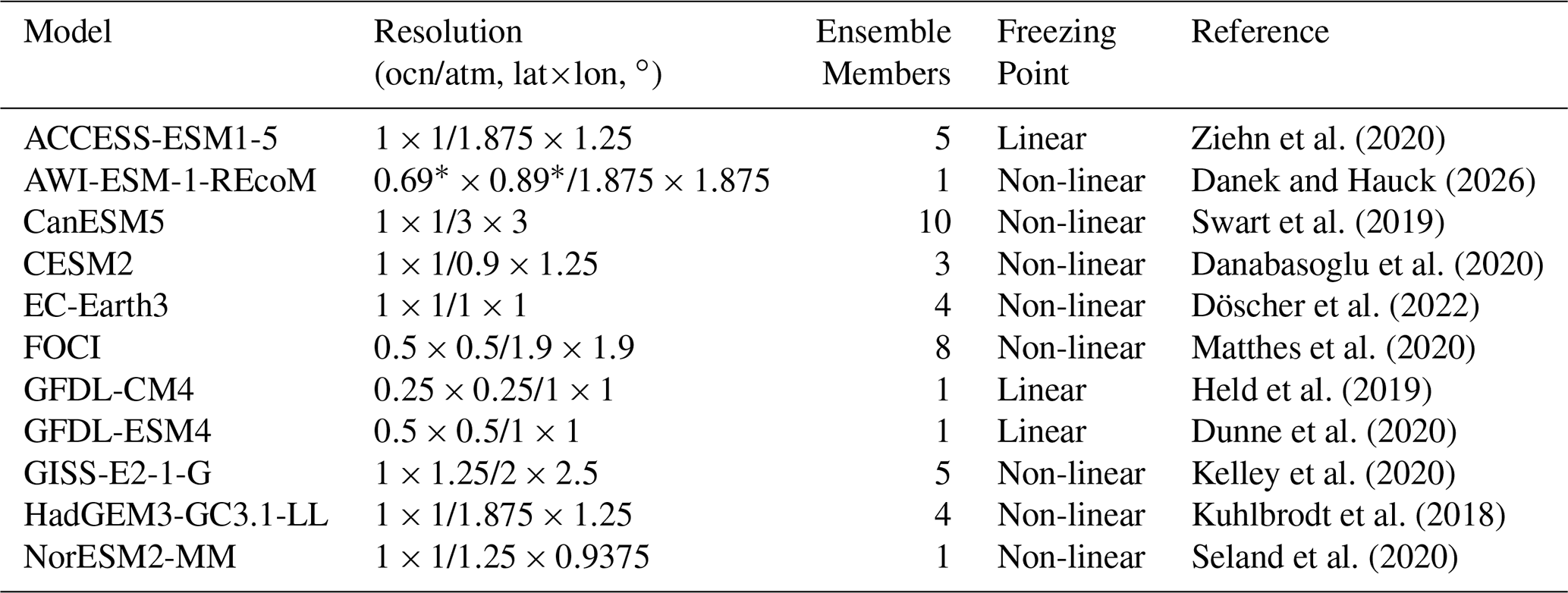
^∗ Global average of unstructured horizontal resolution.

2 Data and Methods

The Tier 1 antwater experiment defined in the SOFIA protocol prescribes a meltwater flux of 0.1 Sv (3154 Gt yr⁻¹) evenly distributed at the ocean surface across all grid cells immediately adjacent to the Antarctic coast. Although this amount of meltwater is larger than contemporary observational estimates of ice shelf basal melt rates (0.035–0.050 Sv, Adusumilli et al., 2020; Davison et al., 2023) or Antarctica's current mass imbalance (0.006–0.016 Sv, Slater et al., 2021), the antwater experiment was designed to produce a robust signal for the purposes of model intercomparison, not to match observations over the historical period. This magnitude of meltwater input is comparable to the projected meltwater flux in the mid-to-late 21st century (e.g., Swart et al., 2023). The idealized nature of the antwater experiment allows us to examine the response to an increase in Antarctic meltwater without the additional interaction with anthropogenic greenhouse gas or aerosol forcing.

Table 1 lists the models that participated in the antwater experiment outlined in the SOFIA experimental design. For models that ran more than one ensemble member, we computed the results as the ensemble mean to reduce the impact of internal variability. For SOFIA, the antwater experiments were branched from each model's CMIP6 piControl (pre-industrial control simulation). The SOFIA protocol requested that the ensembles be generated by branching each member from a different year in the model's piControl run, where the years are chosen to have different phasing of low-frequency ocean variability. Thus, when computing the response for a given variable, each ensemble member is compared with the corresponding time period of the model's CMIP6 piControl run. The time averages of the response are always based on the last 30 years of monthly-mean output of the 100-year-long experiment and the overlapping period of the piControl run, if not stated otherwise. This averaging period was chosen to be long enough to reduce the influence of the initial adjustment to the forcing and internal variability, yielding a quasi-equilibrated upper Southern Ocean. We choose to use overlapping periods from the piControl run for each ensemble member as the baseline, rather than a long-term average, to maintain the sampling across low-frequency ocean variability as outlined in the SOFIA protocol. Statistical significance of the anomalies was computed using a 2-tailed Student's t test. A potentially important consideration in how each model responds to the addition of meltwater is how the ocean model computes the freezing point of seawater. Thus, in Table 1 we note whether the model uses a constant freezing point of seawater, or a linear or non-linear relationship between the salinity and the freezing point of seawater.

As a point of reference we include satellite observations of Antarctic sea ice area (Fetterer et al., 2025) when analyzing the sea ice area mean state across models. While the antwater simulations are under pre-industrial control forcing, and so the sea ice mean state should not necessarily be close to present day conditions, we include the observations to show how far from modern conditions each model may or may not be.

To quantify the effect of additional meltwater on the stratification of the Southern Ocean, we make use of a modified version of the stratification index (SI), as used in Sgubin et al. (2017), Bourgeois et al. (2022) and Weiffenbach et al. (2024). To avoid ambiguity with the abbreviation for “sea ice”, here we denote this as I_strat. This is typically defined as the sum of the difference in potential density referenced to 0 dbar between each depth and the surface in 200 m depth increments down to 2000 m depth. Here, we modify the definition to sum the density in 50 m depth increments down to 500 m depth (after linear interpolation of the density to these depth levels) in order to better capture the stratification around the mixed layer, where we expect the addition of Antarctic meltwater to have the largest effect on sea ice:

$$\begin{array}{}\text{(1)}& I_{\mathrm{strat}}=\sum _{i=\mathrm{1}}^{\mathrm{10}}\mathit{\rho }\left(z_i\right)-\mathit{\rho }\left(z_{\mathrm{0}}\right),\end{array}$$

where z₀ is the ocean surface and $z_i=z_{i-\mathrm{1}}+\mathrm{50}$ m for i=1, …, 10 (units of z in meters).

We computed the deep mixed volume (DMV) as a metric for the amount of open-ocean deep convection that occurs in the Southern Ocean in each model. Following the method of Chen et al. (2023), DMV is calculated by finding all grid cells south of 55° S with a monthly-mean mixed-layer depth (MLD) greater than 2000 m, multiplying the MLD by the area of the grid cell and adding all grid cells. We used the CMIP6 variable “mlotst” for the mixed-layer depth, which is calculated on the model's timestep, and when computing the annual mean, we compute the monthly DMV before taking the annual mean, rather than using the annual mean MLD.

Figure 1 Antarctic annual sea ice area: (a) mean-state in the control run; response as (b) absolute area increase; and (c) percentage change relative to the control run for each of the SOFIA models. Shading denotes the range across ensemble members for the models with more than one ensemble member. Solid colored lines denote each model's ensemble mean. The thick black line denotes the multi-model mean computed by averaging over all ensemble members. The dashed black line shows the average Antarctic sea ice area over the satellite era (1979–2024) as a point of reference (Fetterer et al., 2025).

3 Results

3.1 Sea Ice Response

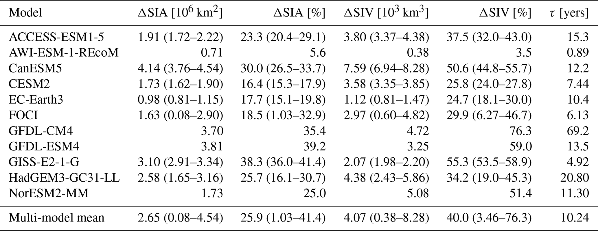
We first examine the mean state of the Antarctic sea ice area and the response to additional Antarctic meltwater in each of the models that have contributed Tier 1 experiment output to SOFIA. The mean-state annual-mean Antarctic sea ice area in the piControl run for each model over the same time period as the antwater experiment is shown in Fig. 1a. The mean-state Antarctic sea ice area ranges from ∼6 million km² in EC-Earth3 to ∼14 million km² in CanESM5, more than a factor of two difference. As a point of reference, the annual-mean observed Antarctic sea ice area from the NSIDC Sea Ice Index over the satellite era (1979–2024) is 8.7 million km². There is a wide range in the response of the Antarctic sea ice area to additional meltwater, with almost no change in AWI-ESM-1-REcoM and a change of ∼4 million km² in CanESM5 and GFDL-ESM4 by year 100 (Fig. 1b). This range in sea ice area response can be explained in part by the differing mean state of the Antarctic sea ice area across the models. When the response of the sea ice area is plotted as a percentage change relative to the Antarctic sea ice area in the control run of each model (Fig. 1c), there is a 20 %–40 % increase in sea ice area relative to the control by year 100 in most models. The exceptions to this are AWI-ESM-1-REcoM, with very little sea ice area change, and GFDL-ESM4 which has a period of unusually large sea ice area change. This large sea ice area response in the GFDL-ESM4 model, particularly from years 50–70, is influenced by a period of strong open-ocean deep convection present during those years in the piControl which creates a large polynya in the Weddell Sea region. The large polynya in the piControl simulation was previously noted in Beadling et al. (2022), with the 100 years of the antwater simulation corresponding to years 101–200 in the piControl shown in their Fig. 5. This polynya is not present in the antwater simulation, and differencing the time series year-by-year accounts for the ∼2.5 million km² variation (dip in sea ice area in piControl (Fig. 1a) becomes a peak in the response (Fig. 1b–c). The role of open-ocean deep convection in the sea ice response is discussed in more detail below. The ensemble-mean changes in total Antarctic sea ice area and sea ice volume averaged over the last 30 years of the 100-year simulations are summarized in Table 2.

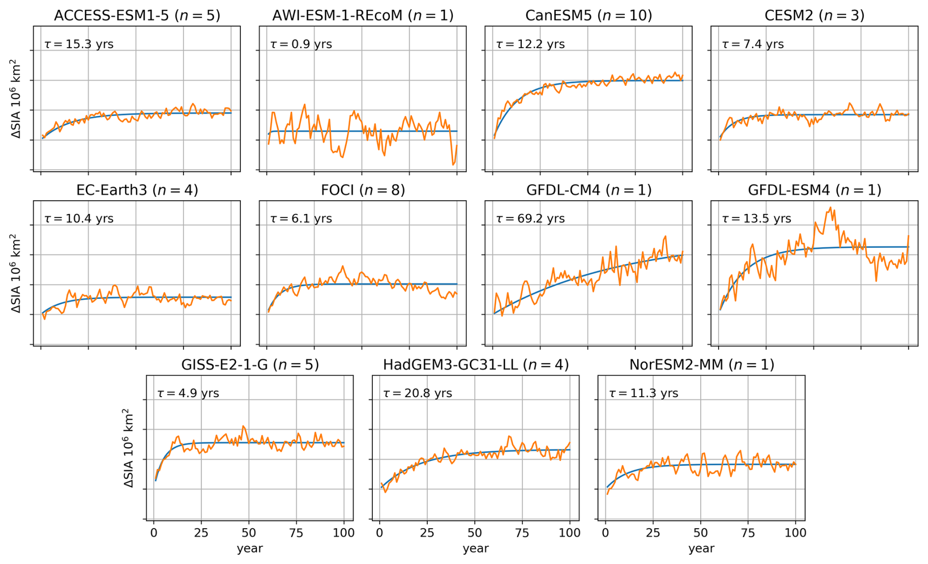
The timescale of the response of the sea ice area to additional Antarctic meltwater also differs between models. In most models, there is an initial rapid increase in sea ice area which later slows and approaches a new equilibrium. However, not all models follow this pattern, with very little change in sea ice area in AWI-ESM-1-REcoM, and an almost monotonic increase over the entire 100 year period in GFDL-CM4. To quantify these differences, we fit an exponential function of the form

$$\begin{array}{}\text{(2)}& \mathrm{\Delta }\text{SIA}=A\left(\mathrm{1}-e^{\frac{-t}{\mathit{\tau }}}\right)\end{array}$$

to the ensemble-mean, annual mean sea ice area response, where A is the amplitude in million km², t is time in years, and τ is a time constant in units of years. τ represents the time to reach 63 % of the final equilibrium value, and the value of τ for each model is given in Table 2. The time constant τ ranges from 0.89 years in AWI-ESM-1-REcoM (in which there is essentially no change in the sea ice area) to 69.2 years in GFDL-CM4, reflecting the almost monotonic increase in sea ice area in that model. Most of the models have τ values between 5 and 20 years, and the multi-model mean value of τ is 10.2 years (see Appendix A for details).

Figure 2 Ensemble-mean seasonal cycle of Antarctic sea ice area for each model (a–k) and the anomaly between antwater and piControl for each model (l). Results are computed as the total Antarctic sea ice area for each month averaged over the final 30 years of the 100 year simulations. Shading denotes the range across ensemble members for the models with more than one ensemble member.

We next examine the mean-state seasonality of the sea ice area and its response to meltwater (Fig. 2). In all models, Antarctic sea ice reaches its minimum area in February–March, and its maximum area in September. However, the annual minimum sea ice area varies from almost zero in EC-Earth3, GFDL-CM4, GFDL-ESM4 and GISS-E2-1-G, to more than 5 million km² in CanESM5. Although it has the largest annual mean Antarctic sea ice area (Fig. 1a), we see that the annual maximum area in CanESM5 (∼ 20 million km²) is similar to several other models (AWI-ESM-1-REcoM, GFDL-CM4, GFDL-ESM4). In most models, the increase in sea ice area is largest around the time of the annual sea ice area maximum in September, with a much smaller increase around the time of the annual minimum in February (Fig. 2l). The multi-model mean difference between the minimum and maximum monthly anomaly is 2.06×10⁶ km². However, in CanESM5 and FOCI the increase in the sea ice area is approximately the same year-round. Particularly the FOCI ensemble (green shading in Fig. 2l) demonstrates the limiting effect of open ocean deep convection, which is present in some of its members, on the winter sea ice response.

Figure 3 Antarctic annual sea ice volume: (a) mean-state in the control run; response as (b) absolute area increase; and (c) percentage change relative to the control run for each of the SOFIA models. Shading denotes the range across ensemble members for the models with more than one ensemble member. Solid colored lines denote each model's ensemble mean. The thick black line denotes the multi-model mean computed by averaging over all ensemble members.

Surface cooling induced by the addition of meltwater from the Antarctic ice sheet can increase not only the areal coverage of sea ice but also its volume. Changes in sea ice volume are important for ocean–atmosphere fluxes of heat, moisture, and carbon as well as biology in this region (e.g., Massom and Stammerjohn, 2010; Gupta et al., 2020; Swadling et al., 2023); thus, we next examine the response of sea ice volume to Antarctic meltwater. Antarctic sea ice volume has a similar large inter-model spread in the piControl mean state as the sea ice area (Fig. 3a). There is also a large inter-model spread in the response to Antarctic meltwater. The total volume of sea ice increases by $\sim \mathrm{8}\times {\mathrm{10}}^{\mathrm{3}}$ km³ in CanESM5, while it is relatively unchanged in AWI-ESM-1-REcoM (Fig. 3b). When plotted as a percentage change, we see that the multi-model mean change in sea ice volume is a 42 % increase (Fig. 3c). The two GFDL models have a much higher and more variable percentage change in sea ice volume. In particular, three of the models with low total sea ice volume in their piControl runs (GFDL-CM4, GFDL-ESM4 and GISS-E2-1-G) show the largest percentage change in both the area and volume of the sea ice.

Table 2 Ensemble-mean absolute and percentage changes in Antarctic sea ice area (SIA) and sea ice volume (SIV), and time constant τ for an exponential fit to the response. The absolute and percentage changes for each model are averaged over the last 30 years of 100 year simulations. Numbers in parentheses denote the minimum and maximum change across ensemble members for the last 30 years for models with more than one ensemble member.

Due to the different sizes of the ensembles between the models used in this study, it is worth considering the role of the ensemble size in assessing the response. In Appendix B we reproduce Figs. 1 and 3 using the first ensemble member only for each model (Figs. B1 and B2). Using a single ensemble member for each model does not substantially change any of the qualitative results described above. Thus, we continue to show ensemble mean responses in the main text, as this reduces the role of internal variability in the response. We further conclude that the spread in the response to the freshwater is dominated by model uncertainty since, firstly, the ensemble spread for a given model is typically smaller than the spread across models and, secondly, removing ensemble members does not significantly alter the multi-model mean.

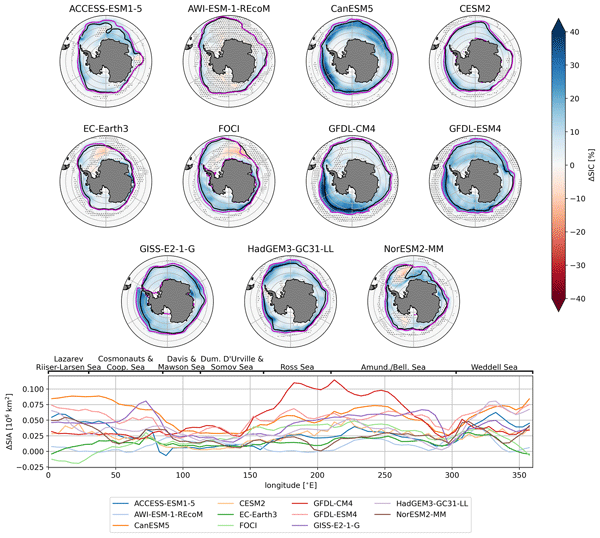
There is a large spread in both the magnitude and spatial pattern of the response of sea ice concentration to the addition of meltwater (Fig. 4). The sea ice concentration increases by ∼40 % in some regions in the CanESM5, GFDL-CM4 and GFDL-ESM4 models. In most models, there is a large change in sea ice concentration near the sea ice edge in the Ross Sea and Amundsen/Bellingshausen Sea regions (between 150–300° E in the lower panel of Fig. 4), with little consistency in the pattern response in other regions. The decrease in sea ice concentration in the Lazarev/Rilser-Larsen Sea region in the FOCI and EC-Earth3 models is due to the development of a region of open-ocean deep convection, leading to the formation of a large polynya. There are also some regions of reduced sea ice concentration that are associated with open-ocean deep convection in the NorESM2-MM model (Weddell and Ross seas) and to an even smaller degree in ACCESS-ESM1-5 and AWI-ESM-1-REcoM. Nevertheless, even in sectors affected by this decrease in sea ice concentration within the ice pack, a northward expansion of the sea ice edge is found.

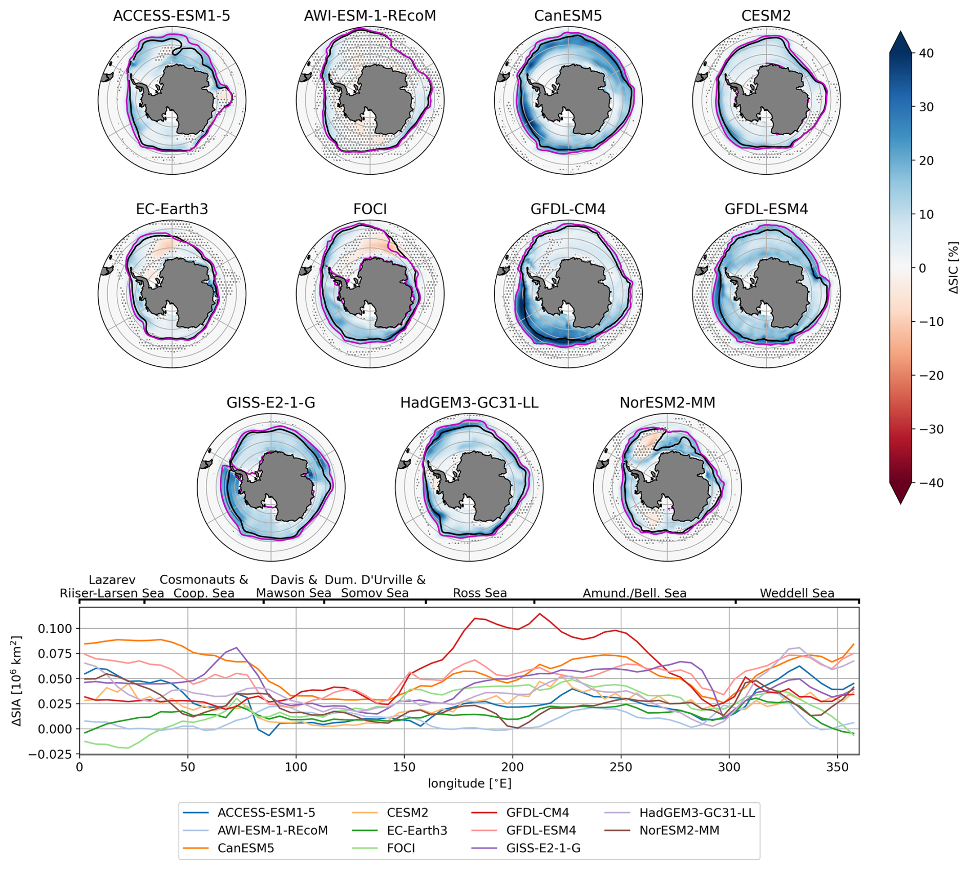
Figure 4 Ensemble-mean sea ice concentration response for each of the models (top three rows). The black and magenta lines denote the annual-mean 15 % concentration contour for the piControl and antwater experiments, respectively. Stippling denotes where the anomaly is not statistically significant at the 95 % confidence level. Bottom row: sea ice area response as a function of longitude. Response is the ensemble-mean difference between the antwater experiment and the piControl binned into 5 degree longitude increments. Approximate longitudinal extents of marginal seas based on the limits proposed in International Hydrographic Organization (2002). Results are averaged over the last 30 years of 100 year simulations.

The spatial response of the Antarctic sea ice volume also varies widely between models (Fig. 5). Several models have a large increase in sea ice volume along the coast in the Indian and Atlantic sectors, extending northward and eastward from the tip of the Antarctic peninsula (300–350° E in the lower panel of Fig. 5). Other than in the Weddell Sea/Antarctic Peninsula region, the change in sea ice volume appears to be more homogeneous across models than that in sea ice area.

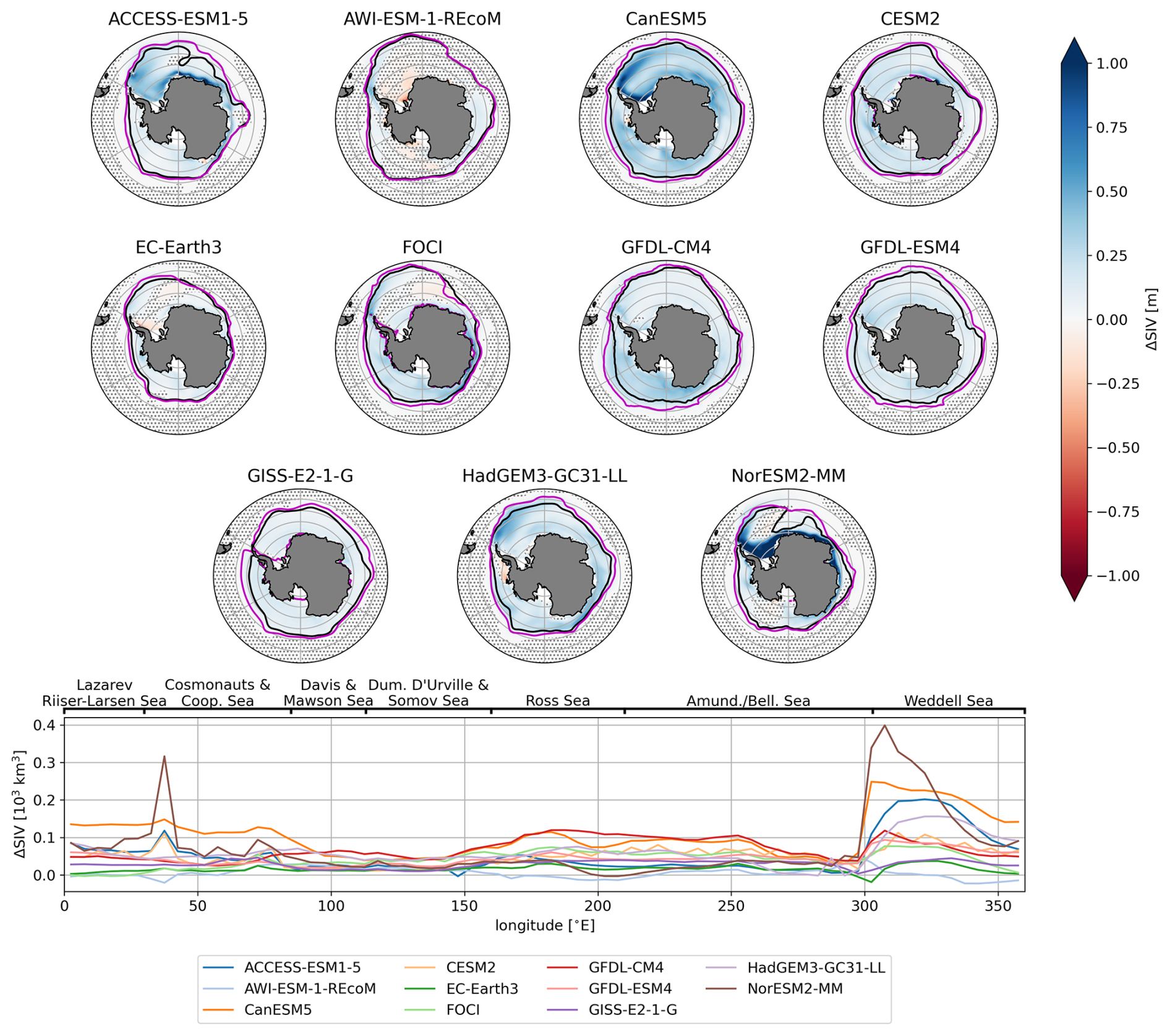
Figure 5 Ensemble-mean sea ice volume response for each of the models (top three rows). The black and magenta lines denote the annual-mean 15 % concentration contour for the piControl and antwater experiments, respectively. Stippling denotes where the anomaly is not statistically significant at the 95 % confidence level. Bottom row: sea ice volume response as a function of longitude. Response is the ensemble-mean difference between the antwater experiment and the piControl binned into 5° longitude increments. Approximate longitudinal extents of marginal seas based on the limits proposed in International Hydrographic Organization (2002). Results are averaged over the last 30 years of 100 year simulations.

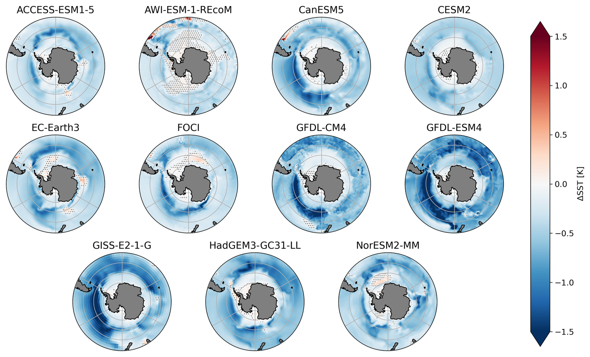
Figure 6 Ensemble-mean annual-mean sea surface temperature response for each of the models. Results are presented as the average over the last 30 years of the 100 year simulations. Stippling denotes where the response is not statistically significant at the 95 % confidence level.

3.2 Ocean Response

To investigate the reasons for the spread between models in the sea ice response, we first examine the response of sea surface temperature (SST) to the addition of freshwater (Fig. 6). There is cooling of the Southern Ocean sea surface in all models, predominantly just beyond the sea ice edge, with a large spread in the magnitude of the cooling. As expected, the models that cool most strongly (CanESM5, GFDL-CM4, GFDL-ESM4 and GISS-E2-1-G) have the largest sea ice concentration and area response (Figs. 1b and 4). There is slight warming of the sea surface in the sea ice-covered region in AWI-ESM-1-REcoM, which is consistent with the weak sea ice response in that model. There are also regions of warming in the FOCI and EC-Earth3 models, consistent with the deep convection that arises in the antwater simulation in those models.

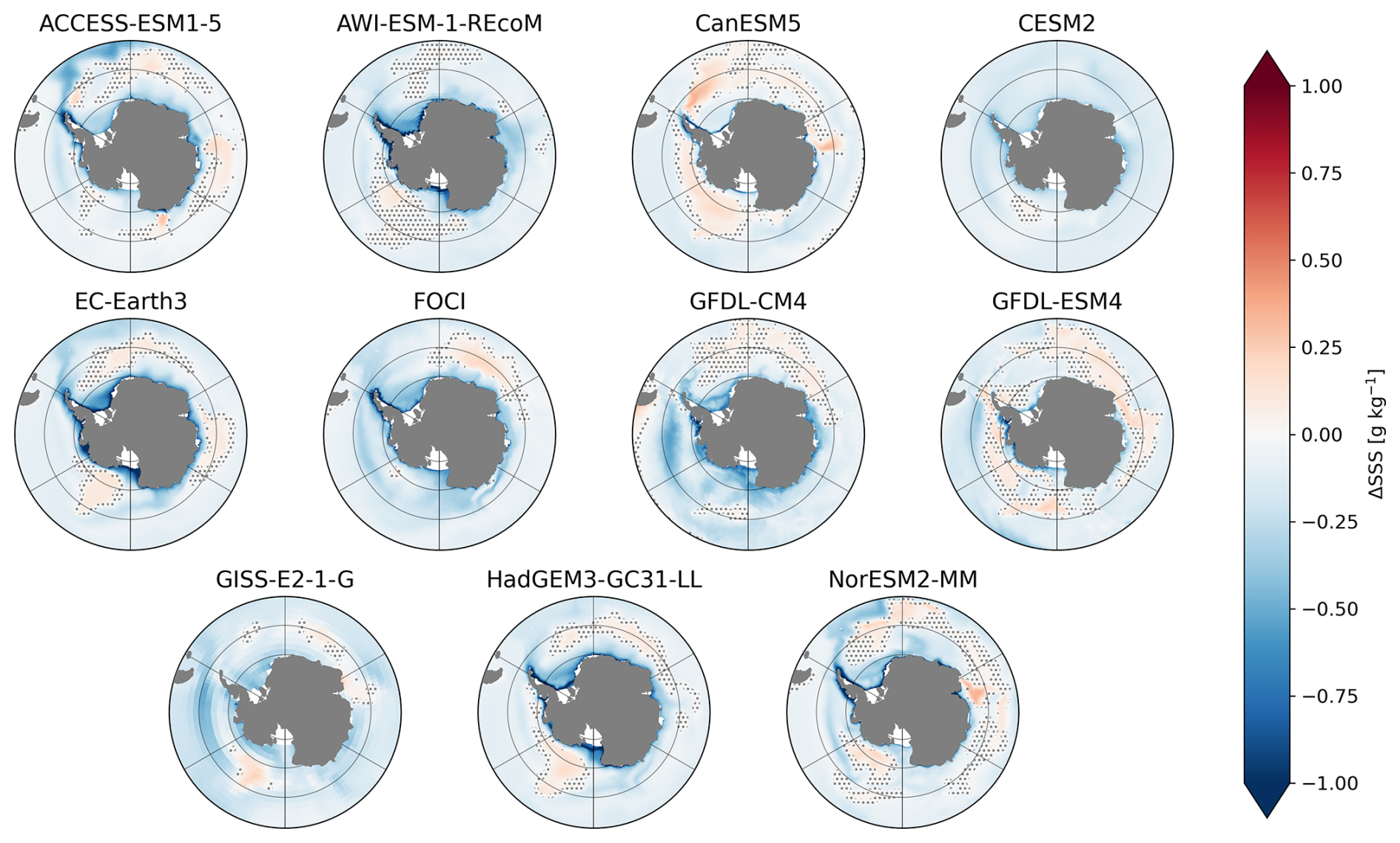
Figure 7 Ensemble-mean annual-mean sea surface salinity response for each of the models. Results are presented as the average over the last 30 years of the 100 year simulations. Stippling denotes where the response is not statistically significant at the 95 % confidence level.

Next, we examine the sea surface salinity response (Fig. 7). There is a wide range in both the spatial pattern and magnitude of the salinity response across models. There is general surface freshening overall, with some models showing regions of increased salinity due to regions of open-ocean deep convection bringing relatively warm, salty water to the surface (EC-Earth3 and FOCI), or increased brine rejection from sea ice formation or decreased freshening due to sea ice melt (CanESM5 and GFDL-ESM4). In several models (ACCESS-ESM1-5, EC-Earth3, FOCI, HadGEM3-GC31-LL, and NorESM2-MM), the flow of the meltwater into the South Atlantic from the tip of the Antarctic Peninsula can be seen, consistent with the increased sea ice volume in that region.

Figure 8 Annual-mean mixed-layer depth response and deep mixed volume (DMV) for the piControl (blue) and antwater (orange) experiments for each of the models. DMV is computed as the product of mixed-layer depth and grid cell area for all grid cells south of 55° S with mixed-layer depth greater than 2000 m. Mixed-layer depth response is the difference between antwater and piControl averaged over the final 30 years of 100-year simulations.

Antarctic sea ice is strongly influenced by regions of open-ocean deep convection (e.g., de Lavergne et al., 2014), since the convection mixes relatively warmer, deeper water up to the ocean surface where it can reduce sea ice cover. CMIP6 models exhibit a large spread in the area and location of open-ocean deep convection in their mean-state (Heuzé, 2021). The study of Chen et al. (2023) examined the deep convection response of the Southern Ocean to Antarctic meltwater in a subset of the SOFIA models used in this study. They found that in general the addition of meltwater reduces the amount of deep convection in the SOFIA models due to the meltwater increasing the stratification of the water column. This increase in stratification should in turn result in an increase in sea ice, and so we hypothesize that models with a large reduction in open-ocean deep convection may have a greater increase in sea ice area or volume. Here, we extend the analysis of Chen et al. (2023) to include four additional models that have contributed simulations to the SOFIA project since that publication. We see a wide range in both the mean state and the response of the total deep mixed volume in the models (Fig. 8). About half of the models have little or no open-ocean deep convection in either the piControl or antwater experiment. Two models, AWI-ESM-1-REcoM and CESM2 have no deep convection at all, and have correspondingly weak sea ice responses. In CanESM5, GFDL-CM4, GFDL-ESM4 and GISS-E2-1-G the addition of Antarctic meltwater shuts off deep convection almost completely. In EC-Earth3, FOCI and HadGEM3-GC31-LL deep mixed volume is reduced for most of the 100 year runs, but regions of deep convection appear in the antwater simulation near the end of the century (in all 4 ensemble members for EC-Earth3, in 3 out of 8 ensemble members for FOCI and in 1 out of 4 ensemble members for HadGEM3-GC31-LL). Finally, in ACCESS-ESM1-5 and NorESM2-MM there are large regions of consistent deep convection throughout both the piControl and antwater experiments throughout the simulation period; however, the DMV is modestly reduced with the addition of meltwater and is accompanied by a corresponding modest increase in the area and volume of sea ice.

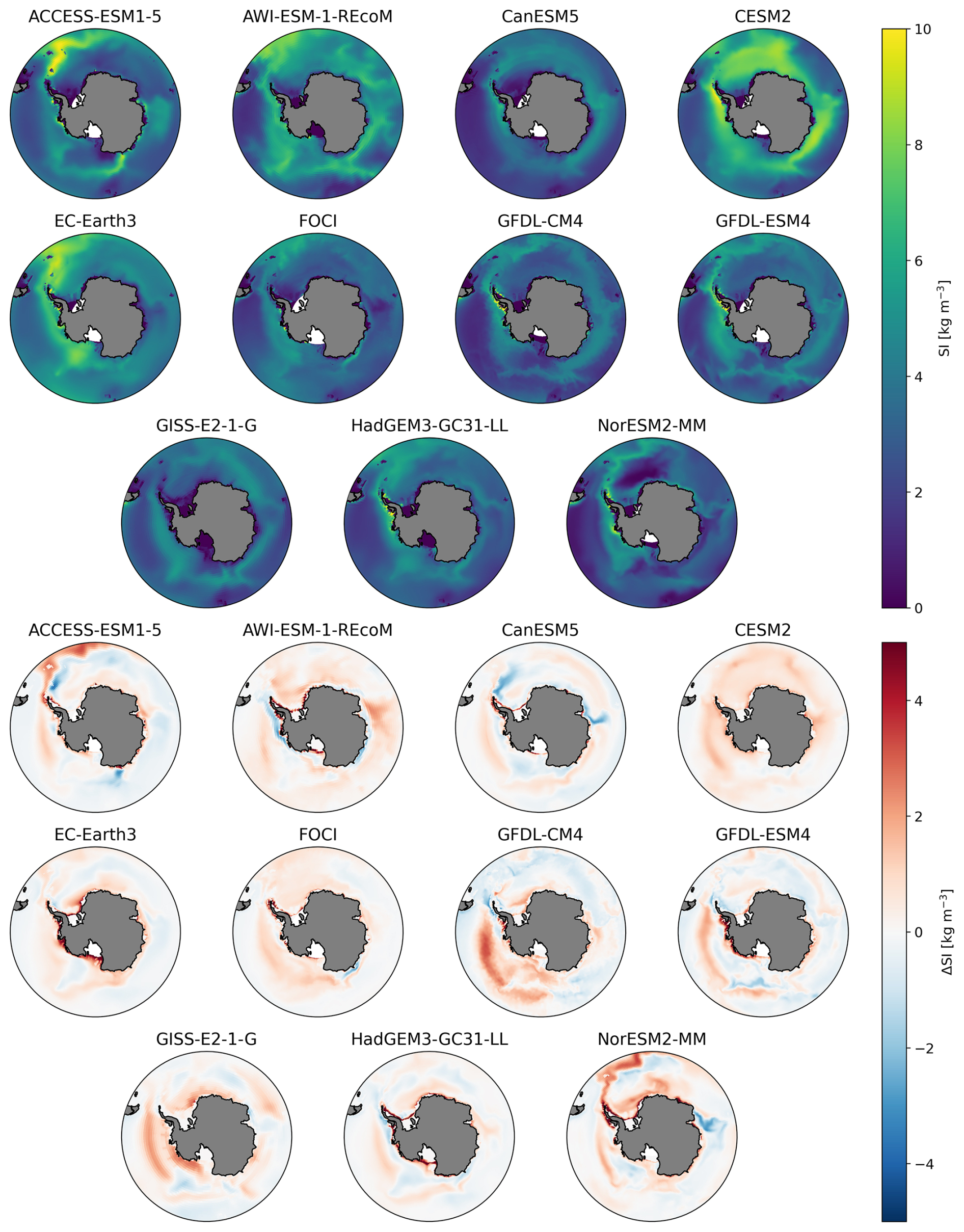
Figure 9 Ensemble-mean stratification index for the piControl (top three rows) and the anomaly between the antwater experiment and the piControl (bottom three rows) for each of the models. A positive anomaly denotes that the water column is becoming more stratified. Results are averaged over the last 30 years of the 100 year simulations.

The addition of Antarctic meltwater affects sea ice by changing the stratification of the water column (e.g., Fogwill et al., 2015; Pauling et al., 2016; Bronselaer et al., 2018). The increase in stratification due to the addition of relatively fresh, less dense water near the surface results in reduced vertical transport of heat from the deeper ocean to the surface, and inhibits open-ocean deep convection (Chen et al., 2023), both of which result in increased sea ice. In addition, dense brine is rejected during sea ice formation, which counteracts the freshening from meltwater and reduces stratification. We next examine the relationship between stratification and the sea ice response across models. Figure 9 shows the modified stratification index (Eq. 1) for both the piControl mean state and the anomaly with the addition of meltwater. We see that there is a wide range in both the magnitude and the spatial pattern of ocean stratification in the mean state, and an overall increase in stratification around the continent with the addition of meltwater. In Fig. 10 we compute the relationships between the Antarctic sea ice area response (ΔSIA) and the piControl stratification index ($I_{\mathrm{strat}}^{\mathrm{CTRL}}$), the change in stratification index (ΔI_strat), the piControl Antarctic sea ice area (SIA_CTRL), and the piControl Antarctic sea ice volume (SIV_CTRL). The relationship between ΔSIA and ΔI_strat is statistically significant (p<0.05), suggesting that the magnitude of the increase in stratification and the sea ice response are tightly coupled. We find no statistically significant relationships at the 95 % confidence level between the Antarctic sea ice area response and the mean-state stratification index, the mean-state sea ice area, or the mean-state sea ice volume. In addition, these relationships help explain some of the intermodel spread in the sea ice response. The two most strongly stratified models, AWI-ESM-1-REcoM and CESM2 (Fig. 10a), have the weakest sea ice response and no deep mixing. We also examined the mean state and response of the stratification seasonally, but found no clear seasonal dependence in the response (not shown).

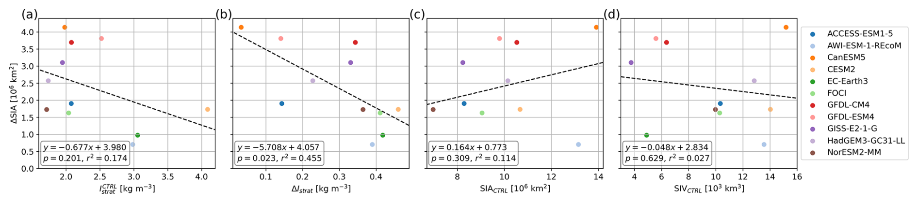
Figure 10 Relationship between the ensemble-mean Antarctic sea ice area response and the ensemble-mean piControl stratification index (a), the ensemble-mean stratification index response (b), the ensemble-mean piControl Antarctic sea ice area (c), and the ensemble-mean piControl sea ice volume (d). The result of a linear least-squares fit to the data and the associated p value are given in the box in the lower left corner of each panel.

4 Discussion

In this study, we present results from the first coordinated multi-model ensemble to examine the response of sea ice to meltwater resulting from Antarctic ice sheet mass loss. We find that multiple factors contribute to the wide inter-model spread in both the temporal and spatial response. The mean-state sea ice area in the piControl simulations for each model explains some of the spread: those models with larger mean-state Antarctic sea ice area also generally (though not always) have a larger change in area in response to meltwater. Furthermore, models with low sea ice volume in their piControl runs typically have the largest changes in sea ice area (see Fig. 10d, aside from CanESM5 and EC-Earth3). This indicates that models with lower mean-state sea ice volume are generally more sensitive to surface cooling driven by the addition of the meltwater and are able to grow a more extensive ice cover because of the reduced insulating effect of the existing sea ice. The fronts associated with the ACC form a natural barrier for northward sea ice expansion (Goosse et al., 2025) limiting the response amplitude in models with larger mean-state sea-ice cover. We found no obvious overall relationship between the method of computing the freezing point of seawater and the sea ice response across models (not shown).

While the spatial response of sea ice concentration and volume (Figs. 4 and 5) varies widely across models, some features are consistent with ocean model simulations of meltwater release (see supporting information of Ashley et al., 2021) showing that meltwater released as far away from the Peninsula as the Ross Ice Shelf front follows the Antarctic coastal and slope currents anticlockwise around the continent, before separating at the tip of the Antarctic Peninsula. Some of the meltwater continues around the Antarctic coast, with the remainder flowing into the Weddell Gyre and out into the Atlantic Ocean, in a pattern similar to the sea ice volume changes in many models shown here. This means that some fraction of much of the meltwater released all around the Antarctic continent will end up being entrained into the Weddell Gyre and flowing into the South Atlantic. Thus, a disproportionate amount of the freshening and stratifying effect of the meltwater will be present in this region.

In most models the sea ice increase is largest in winter and smallest in summer (Fig. 2l). This may be linked to the mechanisms by which meltwater influences sea ice. Sea ice formation requires that the seawater near the surface is cooled to the freezing point. The volume of water that needs to be cooled is dependent on the mixed-layer depth and hence the stratification, and thus the winter sea ice may be more strongly influenced by additional meltwater. Conversely, in summer the sea ice is melting and freshening the surface regardless of the addition of meltwater, and so may be less influenced by meltwater. For CanESM5 and FOCI the seasonality in sea ice area response is less pronounced, however the difference between piControl and antwater is slightly smaller during the melt season, and thus consistent with this mechanism.

Ocean stratification and open-ocean deep convection play important roles in influencing the sea ice response. The response in ocean stratification is strongly related to the sea ice response (Fig. 10b). There is a wide range of mean-state deep convection behavior of the CMIP6 models in the Southern Ocean (Heuzé, 2021), and the subset of CMIP6 models used here also exhibit this range. We find that models without deep convection have relatively weak sea ice responses. GFDL-ESM4, which experiences a period of deep convection in the piControl simulation that is absent in antwater, exhibits a pronounced sea ice area anomaly in the middle of the 100-year simulation (Fig. 1a, b). Furthermore, in the EC-Earth3, FOCI, and HadGEM3-GC31-LL models, open ocean deep convection forms near the end of the antwater simulation, explaining the regions of reduced sea ice area concentration in some ensemble members observed in those models. This region of deep convection is clearly visible in the Lazarev/Riilser-Larsen Sea region in the sea ice concentration response for the EC-Earth3 and FOCI models (Fig. 4). Thus, open-ocean deep convection contributes somewhat to the inter-model spread in the response to Antarctic meltwater.

Although we interpret much of the sea-ice response as arising from the direct oceanic effect of freshwater forcing on upper-ocean stratification, and open-ocean deep convection, the fully coupled nature of these simulations means that atmospheric feedbacks may also contribute to the sea ice response. Freshwater input modifies SST and sea-ice cover, thereby altering the surface albedo of and turbulent heat fluxes over the Southern Ocean, and these surface changes can drive a near-surface atmospheric circulation response. Such circulation anomalies may influence sea ice dynamically, through changes in surface winds driving sea ice transport, and thermodynamically, through changes in near-surface temperature, moisture advection, and air–sea heat exchange. Recent analysis of the atmospheric response in the multi-model ensemble used here (Xu et al., 2025) and similar idealized freshwater-forcing experiments (Beadling et al., 2024) show that Antarctic meltwater can generate a large-scale atmospheric response over the Southern Ocean and beyond. Therefore, while changes in ocean deep convection and stratification provide a physically consistent explanation for much of the simulated response, atmospheric circulation changes may help shape the regional structure of the sea ice concentration anomalies, particularly near the ice edge and in sectors where the sea-ice response is less directly tied to regions of open-ocean convection.

The role of atmospheric feedbacks is particularly relevant when comparing the present Tier 1 experiments with studies that use more realistic freshwater forcing. Zhu et al. (2026), for example, applied spatially distributed Antarctic ice-shelf basal melt forcing for 2006–2016 and found that the coupled atmospheric response can significantly affect the sea-ice response. Their results suggest that the spatial distribution and vertical placement of freshwater forcing can influence not only the local ocean stratification response, but also the atmospheric circulation anomalies that feed back onto sea ice. The idealized protocol used here is therefore best interpreted as a controlled multi-model test of the sensitivity of Antarctic sea ice to a consistent freshwater perturbation, rather than as a complete representation of the regional sea-ice response to realistic Antarctic ice-shelf basal melting. Quantifying the relative roles of ocean stratification, deep convection, and atmospheric feedbacks will require targeted diagnostics, and ideally sensitivity experiments with spatially distributed and depth-dependent freshwater forcing that will be conducted as part of Tier 3 of the SOFIA protocol, discussed further below.

The response of AWI-ESM-1-REcoM is particularly unusual among the models presented here. Despite having high mean-state sea ice area, high sea ice volume and similar ocean stratification to other models, the sea ice response is very weak. This is despite having one of the largest sea surface salinity responses across the models (Muilwijk et al., 2026), and being consistent with the relationship between ΔI_strat and ΔSIA identified in Fig. 10b. This model differs from the others in the ensemble due to having a refined ocean grid close to the Antarctic coastline, with a grid spacing of approximately 20 km near the Antarctic coast, which becomes coarser to the north. Investigation of the reasons for the unusually weak apparent coupling between the ocean and sea ice responses in this model are ongoing.

The models used in this study vary substantially in the horizontal resolution of the atmosphere, ocean and sea ice model components (Table 1). Model resolution has previously been shown to impact both sea ice and the ocean response to Antarctic meltwater. Rackow et al. (2022) showed that the response of Antarctic sea ice to future warming projections is delayed in models with higher-resolution ocean and sea ice components. They attribute this to resolved ocean eddies that increase equatorward heat transport and moderates warming around Antarctica. The study of Beadling et al. (2022) employed the same GFDL-CM4 and GFDL-ESM4 models used in this study and showed that the GFDL-CM4 model, with its higher horizontal resolution of ∼0.25°, better resolves the Antarctic Slope Current which effectively traps the meltwater on the continental shelf, while in the lower-resolution GFDL-ESM4 (∼0.5°) more meltwater is able to escape to the open ocean. The model with the highest resolution ocean-sea ice components used here are, in order, AWI-ESM-1-REcoM, GFDL-CM4, GFDL-ESM4, and FOCI, with the rest all at approximately 1° resolution. There is no clear resolution dependence of the overall sea ice area or volume response, with these four higher-resolution models spanning the full range of responses (Figs. 1 and 3). Nevertheless, as shown in Beadling et al. (2022), model resolution is important for smaller-scale continental shelf processes.

The antwater experiment as defined in the SOFIA protocol (Swart et al., 2023) has many simplifications that should be considered when interpreting the results shown here. In this experiment, the meltwater is evenly distributed across all grid cells immediately adjacent to the Antarctic coast, while in the present-day real world and future projections the meltwater input is higher in the Amundsen/Bellingshausen Sea region (Shepherd et al., 2018; Seroussi et al., 2020). For example Kim et al. (2024) showed that over the period 2003–2020, the Amundsen/Bellingshausen sea sector lost 173.9±6.9 Gt yr⁻¹, while the Antarctic continent overall lost 122±22 Gt yr⁻¹ (the overall loss is smaller than the Amundsen/Bellingshausen Sea loss due to compensating regions of mass gain). Meltwater also only enters the ocean surface in antwater, whereas in reality it enters the ocean through a combination of basal melting of ice shelves, where the meltwater enters the ocean at depth, and calving and subsequent melting of icebergs, where the meltwater enters the ocean far from the coastline. For example, Davison et al. (2023) found that, of the Antarctic ice shelves that lost mass over the period 1997–2021, 68 % of that melt entered the ocean at depth through basal melting, with the remainder entering at the surface through melting of calved icebergs. In addition, the latent heat required to melt the ice is not extracted from the ocean; only the freshening effect is included. The effect of the horizontal and vertical spatial distribution of meltwater input has been examined before in individual modelling studies (e.g., Merino et al., 2018; Mackie et al., 2020a, b; Thomas et al., 2023), with important implications for the local oceanic response in particular, such as different vertical profiles of temperature change over the continental shelf regions.

Future SOFIA experiments will provide an opportunity to further understand the mechanisms linking Antarctic meltwater and sea ice. The SOFIA protocol outlines additional “tiers” of meltwater experiments designed to improve our understanding of the impact of Antarctic mass imbalance in climate models (Swart et al., 2023). Tier 2 consists of experiments with estimates of historical meltwater forcing, and projections of future meltwater input under different emissions scenarios. Tier 3 consists of sensitivity tests to factors such as the spatial distribution and the inclusion of the latent heat effect. At the time of writing, the running and analysis of these additional tiers by multiple modeling groups is ongoing. The results presented here are an important first step in understanding the inter-model spread in the response of Antarctic sea ice to meltwater from the ice sheet, and can be built on by this future work.

The results shown demonstrate that care must be taken when interpreting a given model response to Antarctic meltwater. It has been argued that the inclusion of meltwater due to Antarctic ice-sheet mass loss in historical simulations is important for the models' ability to reproduce the observed sea surface temperature and sea ice trends (Schmidt et al., 2023). However, we have shown here that the magnitude of the Antarctic sea ice response to identical meltwater forcing may vary widely by the end of our 100-year simulations. In Tier 2 experiments of the SOFIA protocol, the effect of Antarctic meltwater due to ice sheet mass loss will be tested under historical and future climate forcing, using best estimates of the historical forcing from Slater et al. (2021), and the ice sheet model output from the Ice Sheet Model Intercomparison Project phase 6 (ISMIP6, Seroussi et al., 2020).

5 Conclusions

The work presented here represents the first coordinated multi-model ensemble analysis of the response of Antarctic sea ice to meltwater entering the Southern Ocean due to mass loss from the Antarctic ice sheet. This meltwater is not included in the coupled climate model simulations that currently form the basis for future climate projections, so understanding the magnitude and uncertainty of its potential impact is important. In response to the addition of 0.1 Sv of meltwater distributed evenly around the Antarctic coast at the ocean surface, the total Antarctic sea ice area increases in the 10 models examined here, but ranges from an annual-mean increase of 0.71–4.14 million km² by the end of 100 years. Similarly, annual-mean sea ice volume increases by between 0.38–7.59×10³ km³ across models. There is no single reason for this large intermodel spread, but a combination of the mean-state Antarctic sea ice area, the mean-state vertical stratification in the ocean, and the mean-state and response of open-ocean deep convection explain much of the variability in response. This work highlights the importance of targeted model intercomparison projects for understanding the climate response to a particular forcing and motivates the running and analysis of additional model experiments defined in the SOFIA protocol that will isolate the role of more detailed aspects of Antarctic meltwater input to the Southern Ocean.

Appendix A: Timescale of the sea ice response

Figure A1 shows the exponential fit to the ensemble-mean sea ice area response for each model, following Eq. (2). For most models, the response of the sea ice area is well described by the exponential model, the exceptions being AWI-ESM-1-REcoM and GFDL-ESM4. AWI-ESM-1-REcoM has almost no change in the sea ice area with the addition of meltwater, so the exponential fit to the response is not meaningful. GFDL-ESM4 has large variability, suggesting that the exponential model does not fit the data well, due to the presence of a large open-ocean polynya in years 50–70, as discussed in the main text.

Figure A1 Ensemble-mean Antarctic sea ice area response for each model with an exponential fit to each curve following Eq. (2). The time constant τ is given for each model. n denotes the number of ensemble members in each model.

Appendix B: Single ensemble member sea ice response

Different numbers of ensemble members were run for each model that contributed output to the antwater SOFIA experiment, with several models running only one ensemble member. This means that comparing the ensemble-mean sea ice responses across models in Figs. 1 and 5 is not a direct comparison. Thus, in Figs. B1 and B2 we compute the sea ice area and volume responses, respectively, using the first ensemble member from each model (variant label r1i1p1f1 or r1i1p2f1 depending on the convention used in each model). We see that the responses are qualitatively similar to those seen in the ensemble mean, with the response of the sea ice area ranging from ∼0 to ∼4 million km² by the end of the century (Fig. B1b) and the sea ice area in most models increases by 20 %–40 % by the end of the century (Fig. B1c). Similarly, the sea ice volume response ranges from between ∼0 and $\sim \mathrm{7.5}\times {\mathrm{10}}^{\mathrm{3}}$ km³ (Fig. B2b) and sea ice volume increases by 25 %–90 % in most models as a percentage of the piControl mean state (Fig. B2c).

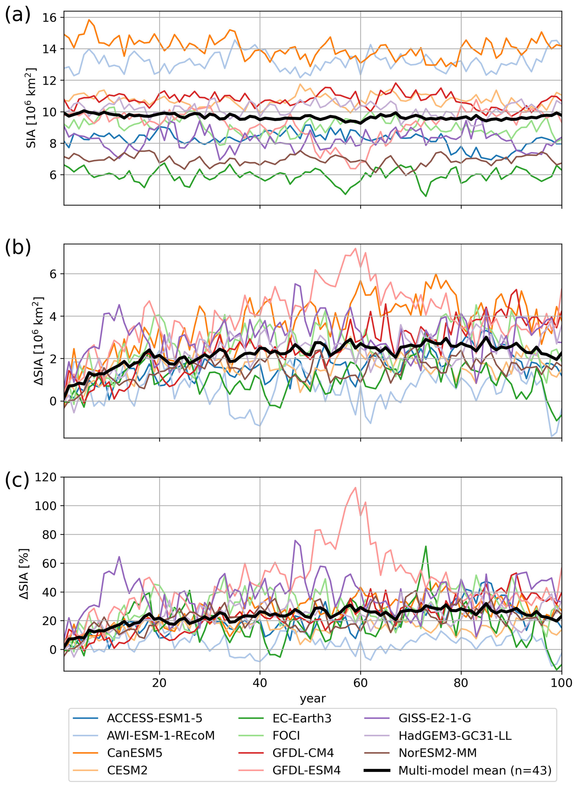
Figure B1 Antarctic sea ice area (a): mean state in the control run, and response as (b) absolute area increase and (c) percentage change relative to the control run for each of the SOFIA models for the first ensemble member in each model. Light-colored lines denote individual ensemble members. Solid colored lines denote each model's ensemble mean.

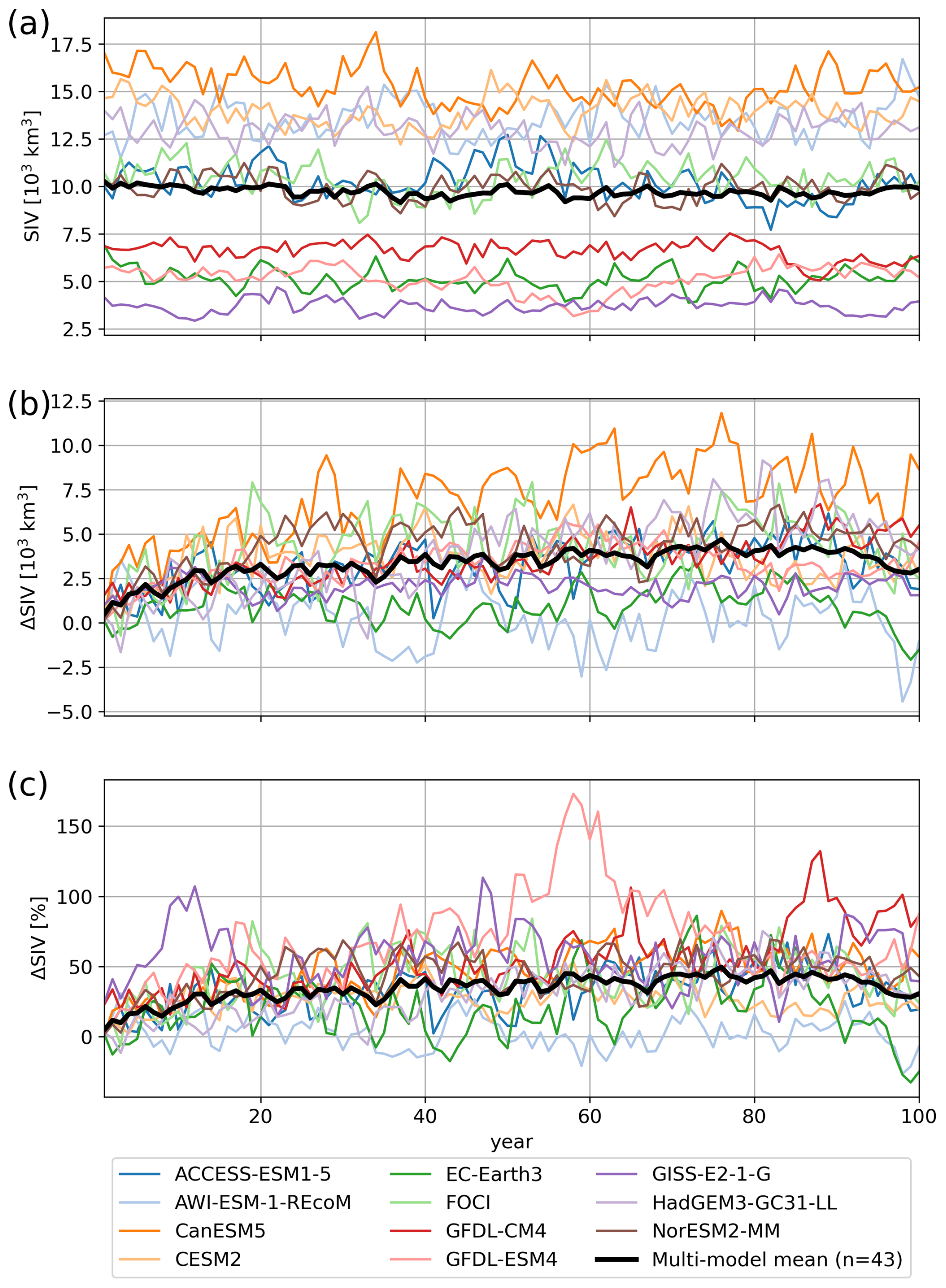
Figure B2 Antarctic sea ice volume (a): mean state in the control run, and response as (b) absolute volume increase and (c) percentage change relative to the control run for each of the SOFIA models for the first ensemble member in each model. Light-colored lines denote individual ensemble members. Solid colored lines denote each model's ensemble mean.