Parameterizing tidal-water intrusions in long-term Antarctic ice-sheet projections

The Antarctic Ice Sheet (AIS) is expected to be the dominant contributor to sea-level rise in the coming centuries. However, this contribution is deeply uncertain due to the lack of understanding of some fundamental processes influencing ice-sheet dynamics. A key question is the extent to which submarine melting takes place at the transition between grounded and floating ice. Traditionally, in continental-scale ice-sheet modelling, this area has been treated as an abrupt transition or grounding line with suppressed or strongly limited submarine melting upstream. However, several lines of evidence challenge this view. In many places, changes in ocean tides lead to back and forth migrations of the grounding line over a broad grounding zone and can cause intrusion of warm ocean waters several kilometres upstream of the grounding line, allowing for submarine melting there. Here, we propose a simple parameterization to represent the effect of tidally-controlled migrations of the grounding line and tidal-water intrusion in submarine melting in continental-scale ice-sheet models. We calibrate the magnitude of the parameter controlling the extent of oceanic water intrusions against the observational evidence as inferred from differential interferometry synthetic aperture radar. We use a three-dimensional ice-sheet model to investigate the impact of this parameterization on Antarctic ice-sheet projections under two high-emission climate scenarios extending to the year 3000. Our results show that increasing the extent of tidal intrusion, reinforced by dynamic feedbacks, leads to stronger and more widespread grounding-zone retreat under warming scenarios, and consequently ice-stream acceleration, ice-shelf thinning and debuttressing. This implies larger sea-level contributions compared to the usual treatment of melt at the grounding line and should be accounted for in future projections.

1 Introduction

The Antarctic Ice Sheet (AIS) contains an ice volume of approximately 58 m of sea-level equivalent (SLE; Morlighem et al., 2020). Over the past two decades (2002–2022), an average of 127±23 Gt yr⁻¹ of ice has been lost (Diener et al., 2021; Hanna et al., 2024). This loss is concentrated in the West Antarctic Ice Sheet (WAIS; Greene et al., 2022; Otosaka et al., 2023) and is largely due to enhanced submarine melting and thinning of ice shelves in this area (Shepherd et al., 2019), which has led to a reduction in the ice-shelf buttressing of the ice sheet, acceleration of the ice flow, and increasing ice discharge (Miles and Bingham, 2024). The AIS will likely become the dominant contributor to sea-level rise in the next centuries with contributions reaching 30 cm  SLE by 2100 and up to 4.4 m  SLE in 2300 (Seroussi et al., 2020, 2024).

Model studies agree in pointing to ice-ocean interactions as the main driver of ice loss via enhanced sub-shelf melting and calving (Turney et al., 2020; Bett et al., 2024; Coulon et al., 2024; Juarez-Martinez et al., 2024; Coulon et al., 2025; Fricker et al., 2025). The incomplete understanding of these and other fundamental processes influencing ice-sheet dynamics, the spread in the representation of these processes, and the potential tipping behaviour of the AIS imply that the future contribution to sea-level rise is deeply uncertain (Fox-Kemper et al., 2021; Coulon et al., 2025). For high-emission scenarios, the sea-level contribution (SLC) by 2300 within the Ice Sheet Model Intercomparison Project (ISMIP6) ranges from −0.6 up to 4.4 m  SLE (Seroussi et al., 2024). The upper-range values result from a collapse of the WAIS, where sectors such as the Amundsen Sea Embayment are highly prone to destabilization through enhanced submarine melting (Paolo et al., 2023; Alevropoulos-Borrill et al., 2024; Hill et al., 2024). Large areas of the WAIS are grounded on retrograde bedrock and therefore potentially subject to the marine ice-sheet instability (MISI; Weertman, 1974; Schoof, 2007), which underlies the high-range estimates of ISMIP6 (Seroussi et al., 2024): when the grounding line (GL), the location where grounded ice becomes afloat, of a marine ice sheet retreats over a retrograde bedrock, the ice thickness at the GL increases. Because ice flux at the GL increases nonlinearly with ice thickness, this results in higher ice discharge, promoting further retreat of the GL, initiating a positive feedback loop that can lead to unstable and potentially rapid retreat of the ice sheet (Pattyn, 2018).

A critical issue in this context is the treatment of submarine melting at the GL. Traditionally, it has been considered to behave as a hydraulic barrier to seawater intrusion beneath grounded ice due to the large horizontal hydropotential gradient imposed by the increasing ice thickness upstream (Robel et al., 2022). Therefore, it has been conceived as a semi-fixed, abrupt transition from grounded to floating ice that migrates only over short distances (100–200 m) during the tidal cycle as it maintains hydrostatic equilibrium (Rignot et al., 2011), with suppressed or strongly limited submarine melting upstream, under ice that does not satisfy the flotation criterion.

However, several lines of recent evidence challenge this view, suggesting that warm ocean waters can intrude several kilometres upstream of the GL (e.g. Chen et al., 2023; Rignot et al., 2024). On one hand, subglacial water is discharged to the ocean close to the GL. Where this cold but fresh water meets warm, salty ocean water, the denser warm and salty ocean water forces the lower density freshwater to rise, creating a salty wedge that can intrude horizontally upstream of the GL (MacGregor et al., 2011; Horgan et al., 2013; Milillo et al., 2019; Warburton et al., 2020; Robel et al., 2022). In addition, the GL migrates back and forth with changes in oceanic tides over much larger distances than those predicted by hydrostatic equilibrium. Tidally controlled migration of the GL by 2–18 km has been documented in several regions such as Pine Island Glacier (Milillo et al., 2017), Thwaites Glacier (Milillo et al., 2019), the Getz Ice Shelf (Mohajerani et al., 2021), the southern Ronne Ice Shelf (Freer et al., 2023), the Amery Ice Shelf (Zhu et al., 2025) and Berry Glacier (Chen et al., 2025). Furthermore, there is evidence for tidally-controlled intrusions of relatively warm ocean water by up to 16 km below grounded ice during (high) spring tides in the Amery Ice Shelf (Chen et al., 2023) and by 6–12 km in the Thwaites glacier (Rignot et al., 2024). Similarly, the GL migrates over a zone of 2–6 km in Petermann Glacier in the northwest of Greenland (Ciracì et al., 2023) and over almost 3 km in Jakobshavn Isbræ in the west of Greenland (Kim et al., 2024). These migrations of the GL lead to the definition of a region called the grounding zone (GZ; Parizek, 2024; Rignot et al., 2024). The intrusion of salty ocean water beneath the ice sheet leads to ice melt by delivering high amounts of ocean heat to zones where, on average, ice can be considered grounded. Melting rates of as much as 50 m yr⁻¹ have been found within the GZ, yielding much higher values than those observed in the adjacent ice shelf (Milillo et al., 2019; Rignot et al., 2024).

Grounding-line retreat can easily be triggered by basal melting in its vicinity in response to oceanic thermal forcing (Arthern and Williams, 2017; Reese et al., 2018; Seroussi and Morlighem, 2018; Parizek, 2024). During the past decade, allowing for submarine melting at even partially floating grid points was thought to lead to an overestimated GL retreat in response to oceanic forcing (Seroussi and Morlighem, 2018; Robel et al., 2022). However, in light of the evidence above, this view is changing. Several studies have actually linked the difficulties of current ice-sheet models to reproduce features such as the ice loss during recent decades or the sea-level highstands from previous interglacials with the lack of submarine melting within the GZ (Chen et al., 2023; Bradley and Hewitt, 2024; Rignot et al., 2024). An increased model sensitivity would have implications for future ice-volume and sea-level projections, but except for a few limited exceptions (e.g. Parizek et al., 2013; Robel et al., 2022; Poinelli et al., 2026) this has not been studied in depth.

In view of these results, a revision in the representation of submarine melting in ice-sheet models has been proposed by adopting schemes that include melting upstream of the GL. Gadi et al. (2023) used a very high-resolution two-dimensional ocean-ice model to calculate submarine melt rates as a function of the GZ length and ocean thermal forcing. Melt rates were found to increase sub-linearly with the GZ length. However, the GZ length in this study was treated as a tunable parameter rather than as a variable predicted by the model.

Wilson et al. (2020) developed a theory of layered seawater intrusion in laterally-confined subglacial channels. Robel et al. (2022) generalized this theory to include subglacial hydrology as a macroporous water sheet over impermeable beds and as microporous Darcy flow through permeable till. Seawater intrusion upstream of the GL was predicted to be limited to just several metres for permeable till, but capable of reaching tens of kilometres over flat or retrograde impermeable beds. In the first case, projections of marine ice-sheet volume loss increased by 10 %–50 % (Robel et al., 2022); for kilometric-scale intrusions, projected ice-volume loss can more than double. Again, the GZ length was treated as a tunable parameter.

Robel et al. (2022) derived an expression for the scale of the intrusion length, which was found to depend on the presence of subglacial channels, the nature of the bed (i.e. deformable bed or till versus hard bed), the porosity, the bed topography (slope), the regime of basal hydrology, the thickness of the seawater layer under the ice, the upstream velocity of the subglacial discharge, and the degree of obstruction by obstacles. Observational studies have confirmed many of these dependencies and included others such as the ice-flow velocity (Brancato et al., 2020; Milillo et al., 2022; Chen et al., 2023; Zhu et al., 2025). Many of these variables are, however, not straight-forward observables. Although these studies provide a valuable theoretical framework for understanding seawater intrusion beneath ice sheets, they do not explicitly consider tidal pumping as a driving mechanism for intrusion. Nevertheless, their formulations offer a useful foundation for investigating seawater intrusion processes regardless of whether they are tidally driven. Furthermore, their representation in state-of-the-art continental-scale ice-sheet models remains challenging, especially when it comes to subglacial hydrology. Robel et al. (2022) introduced an equation that represents the melt upstream from the GL as being proportional to the ocean-induced basal melting at the GL, where upstream melting decreases linearly to zero at a specified distance L upstream. This approach allows for a first-order representation of melt due to tidal intrusions. It is clear though, that L may vary spatially and would depend on the factors listed above. A critical issue is therefore how to determine the length of the GZ with such an approach.

In this study, we propose a simple parameterization of submarine melting that accounts for the length and location of the GZ based on topographical features. This parameterization is dependent on a single parameter that can be estimated from the observational evidence. Melting is then calculated as a spatially weighted melt distribution between grounded and floating ice. To assess the influence of this parameterization, we investigate the sensitivity of the AIS response to the length of the GZ under a future high-emission scenario with the ice-sheet model Yelmo.

This work is structured as follows. In Sect. 2 the ice-sheet model used and the experimental setup are described, together with the description of the parameterization. In Sect. 3, the results of the experiments are presented with special emphasis on the effects of ocean warming and GZ expansion on sea-level contributions. In Sect. 4 we discuss these results comparing them with similar studies. Finally, in Sect. 5 conclusions from this study are drawn.

2 Methodology

2.1 Ice-sheet model setup

In this study, we use the Yelmo ice-sheet model (Robinson et al., 2020) with a horizontal resolution of 16 km (grid of 381 cells × 381 cells) and 10 vertical layers. Yelmo has been tested in benchmark experiments, e.g. EISMINT and MISMIP (Robinson et al., 2020). It has been applied in different domains, including the Laurentide Ice Sheet (Moreno-Parada et al., 2023), the Greenland Ice Sheet (Bochow et al., 2023; Gutiérrez-González et al., 2026), and the AIS (Blasco et al., 2021; Juarez-Martinez et al., 2024), and participated in ISMIP6-2300 (Seroussi et al., 2024).

All experiments presented assume that ice dynamics follow Glen's flow law, relating stress deviatoric tensors with stress rate tensors through an exponent n, defined for this study as 3, and a rate factor $A^{\prime }=EA\left(T^{\prime }\right)$ which follows an Arrhenius law. This law is dependent on the temperature relative to the pressure melting point T^′, and an enhancement factor E, that takes into account different deformation regimes (Greve and Blatter, 2009). These enhancement factors have been chosen as 1.0, 1.0, and 0.7 for the shear, stream, and shelf regions, respectively. The velocity field is computed using the higher-order depth-integrated viscosity approximation (DIVA; Robinson et al., 2022). Basal stress τ_b is implemented as a regularized Coulomb power law (Joughin et al., 2019), given in terms of the basal velocity ${\mathit{u}}_{\mathrm{b}}=(u_{\mathrm{b}},v_{\mathrm{b}})$ as:

$$\begin{array}{}\text{(1)}& {\mathit{\tau }}_{\mathrm{b}}=-c_{\mathrm{f}}N{\left({\displaystyle \frac{\left|{\mathit{u}}_{\mathrm{b}}\right|}{\left|{\mathit{u}}_{\mathrm{b}}\right|+u_{\mathrm{0}}}}\right)}^{\mathrm{q}}{\displaystyle \frac{{\mathit{u}}_{\mathrm{b}}}{\left|{\mathit{u}}_{\mathrm{b}}\right|}}\end{array}$$

with the exponent q=0.2 as suggested from laboratory experiments by Zoet and Iverson (2020) and used in other Yelmo studies (Moreno-Parada et al., 2023; Blasco Navarro et al., 2024), and u₀=100 m yr⁻¹ being an empirical threshold speed below and above which viscous and Coulomb friction are obtained, respectively (Zoet and Iverson, 2020). The dimensionless parameter c_f represents the frictional properties of the bedrock and is optimized during the spin-up as by Juarez-Martinez et al. (2024). The effective pressure N depends on the basal hydrology, which follows from a local energy balance and a fixed till drainage rate (Bueler and van Pelt, 2015):

$$\begin{array}{}\text{(2)}& N=min\left\{P_{\mathrm{o}},N_{\mathrm{0}}\left[{\left({\displaystyle \frac{\mathit{\delta }{P}_{\mathrm{o}}}{N_{\mathrm{0}}}}\right)}^{\mathrm{s}}{\mathrm{10}}^{\frac{e_{\mathrm{0}}}{C_{\mathrm{c}}}(\mathrm{1}-s)}\right]\right\}\end{array}$$

where N₀ = 1000 Pa is the reference effective pressure, P_o is the overburden pressure of ice, e₀=0.69 is the reference void ratio (for N=N₀), $s=H_{\mathrm{w}}/H\mathrm{w},max$ is the ratio between the height of basal water content and the maximum height allowed (2 m in this case) and C_c=0.12 is the till compressibility. Also, the fraction of overburden pressure for saturated till is set to δ=0.8.

Calving is parameterized through the von Mises-like eigenvalue scheme from Lipscomb et al. (2019), with the parameter values of k_t = 0.0025 $\mathrm{m}{\mathrm{yr}}^{-\mathrm{1}}{\mathrm{Pa}}^{-\mathrm{1}}$ and w₂=25. This calving law is analogous to the von Mises calving law (Morlighem et al., 2016), but stress is used in place of the strain rate and the parameters are empirical coefficients.

Submarine melting is parameterized through the generalized non-local basal melt parameterization described by Jourdain et al. (2020) and used within ISMIP6 (Seroussi et al., 2020). This parameterization takes into account not only the local thermal forcing, but also the effects of the average forcing over the cavity beneath a given ice shelf. The sub-shelf basal melting of floating ice ${\dot{b}}_{\mathrm{f}}(x,y)$ is given by:

$$\begin{array}{}\text{(3)}& \begin{array}{rl}{\dot{b}}_{\mathrm{f}}(x,y)& ={\mathit{\gamma }}_{\mathrm{0}}{\left({\displaystyle \frac{{\mathit{\rho }}_{\text{sw}}{c}_{\text{pw}}}{{\mathit{\rho }}_i{L}_{\mathrm{i}}}}\right)}^{\mathrm{2}}\left(T_{\text{F}}(x,y,z_{\text{draft}})+\mathit{\delta }{T}_{\text{sector}}\right)\\ & \times |\langle T_{\text{F}}{\rangle }_{\text{draft}\in \text{sector}}+\mathit{\delta }{T}_{\text{sector}}|\end{array}\end{array}$$

where $T_{\text{F}}(x,y,z_{\text{draft}})$ is the thermal forcing (the oceanic temperature relative to the pressure melting point, dependent on salinity) at the ice-ocean interface, with z_draft being the elevation of the ice shelf base, ρ_sw is the density of ocean water, L_i the latent heat of fusion of ice and c_pw the specific heat of the ocean water. δT_sector is a temperature correction to reproduce the observed ice thickness (see Sect. 2.3) and 〈T_F〉_{draft∈sector} represents the thermal forcing averaged over all ice shelves contained in each of the 18 drainage basins in which the Antarctic domain is divided (Jourdain et al., 2020).

Basal melting modifies the buoyancy of the cavity through the production of relatively fresh meltwater. The resulting buoyancy-driven circulation redistributes heat and freshwater throughout the cavity, influencing ocean temperatures and melt rates far from the location where the initial melting occurred, which explains the non-local character of the process and the parameterization. As noted by Jourdain et al. (2020), although the calibration could be performed independently for each cavity, ice-sheet models have evolving cavities whose present-day ice shelves and flows may not match observations. Moreover, initially separated ice shelves can merge over time, causing melt discontinuities if parameters are calibrated at the drainage-basin scale. Jourdain et al. (2020) therefore calibrate parameters at the larger sector scale. The parameter γ₀ is a heat-exchange factor with a value of 14 500 m yr⁻¹ corresponding to the medium value used in the ISMIP6 protocol (Seroussi et al., 2020).

Yelmo is coupled to FastIsostasy, a 2D Glacial Isostatic Adjustment (GIA) model that accounts for the lateral variability of the solid Earth structure and computes the spatially heterogeneous sea-surface elevation resulting from gravitational anomalies (Swierczek-Jereczek et al., 2024). For our simulations, we consider two layers for representing the Earth's inner structure: the lithosphere and the mantle, with densities of 3200 and 3400 kg m⁻³, respectively. The laterally-variable rheology (lithospheric thickness and mantle viscosity) and Earth structure were obtained from Lloyd et al. (2024). The barystatic sea level evolves according to the AIS topography, as described by Goelzer et al. (2020).

Finally, although we used a 16 km grid as the default configuration throughout the study, we performed an additional set of experiments using several H_t values at 8 and 32 km resolutions to assess the influence of grid resolution (see Sect. 4).

2.2 Parameterization of subgrid tidal intrusion

Leguy et al. (2021) introduced the partial melt subgrid parameterization (PMP) to account for basal melting at partially floating grid cells containing the GL (see also Seroussi and Morlighem, 2018). Here, we introduce a modification of PMP, hereafter the Partial Melt Parameterization with Tides (PMPT), to account for submarine melting resulting from tidal water intrusions under grounded ice. With this approach, we do not intend to represent vertical motion of tides, but rather the extent of the tidal intrusions. Also, bending stresses at the GL, which lower the ice below flotation near the GZ and raise it farther downstream (Gadi et al., 2025), are not captured by our parameterization. Tsai and Gudmundsson (2015) demonstrated that GL migration is not proportional to the height of tides, but rather nonlinear and asymmetrical, favoring upstream migration. In addition, Rosier and Gudmundsson (2020) and Zhu et al. (2025) demonstrated that vertical motion of between 2 and 3 m can make the GL migrate several kilometers horizontally.

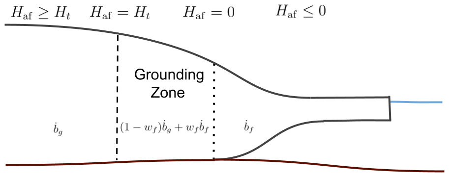
Figure 1 Schematic representation of a marine ice-sheet section to illustrate the PMPT parameterization. The slope of the ice surface and bedrock determine the distance upstream of the GL (corresponding to H_af=0) at which H_af=H_t and therefore the extent of tidal seawater intrusion or GZ length.

In the PMPT approach, we make the important assumption that the intrusion distance upstream from the grounding line, L, can be expected to be inversely proportional to the along-flow gradient of ice thickness above flotation, i.e.,

$$\begin{array}{}\text{(4)}& L\propto {\left({\displaystyle \frac{\partial H_{\text{af}}}{\partial x}}\right)}^{-\mathrm{1}}\end{array}$$

where $H_{\text{af}}=H-\frac{{\mathit{\rho }}_{\text{sw}}}{{\mathit{\rho }}_{\mathrm{i}}}max(z_{\text{sl}}-z_{\text{bed}},\mathrm{0})$ is the ice height above flotation, H is the ice thickness, z_sl is the sea surface elevation, z_bed is the bedrock elevation and x can be considered the coordinate along a flowline from the GL (x=0) increasing in the upstream direction. By definition H_af→0 as x→0. In other words, we assume that the intrusion length is small when H_af increases rapidly moving upstream, and the intrusion length is large when H_af increases slowly moving upstream (Fig. 1). Such an assumption is consistent with theory (Robel et al., 2022), see Appendix A for details. This relationship implies that we can define a threshold ice height above flotation, H_t, that corresponds to the intrusion length, $H_{\mathrm{t}}=H_{\text{af}}(x=L)$.

In this way, we can avoid defining the intrusion length directly, since this is challenging to represent in the model, while H_af is a variable that is readily available. Thus we can define a weighting function for the fraction of ocean-driven melt to be applied. For the sake of simplicity, we obtain it as:

$$\begin{array}{}\text{(5)}& w_{\mathrm{f}}=\mathrm{1}-{\displaystyle \frac{H_{\text{af}}}{H_{\mathrm{t}}}},\end{array}$$

which is valid for $\mathrm{0}<H_{\text{af}}<H_{\mathrm{t}}$. With this equation, the amount of melting reduces linearly as H_af→H_t. To calculate the basal melting at a given location then, we use the following equation:

$$\begin{array}{}\text{(6)}& \dot{b}=\left\{\begin{array}{ll}{\dot{b}}_{\mathrm{g}},& \text{if}{H}_{\text{af}}\ge H_{\mathrm{t}},\\ {\dot{b}}_{\mathrm{f}},& \text{if}{H}_{\text{af}}\le \mathrm{0},\\ (\mathrm{1}-w_{\mathrm{f}}){\dot{b}}_{\mathrm{g}}+w_{\mathrm{f}}{\dot{b}}_{\mathrm{f}},& \text{if}\mathrm{0}<H_{\text{af}}<H_{\mathrm{t}}.\end{array}\right.\end{array}$$

where ${\dot{b}}_{\mathrm{f}}$ is the basal melting for floating ice as introduced in Eq. (3) and ${\dot{b}}_{\mathrm{g}}$ denotes basal melting for grounded ice resulting from basal friction heat and geothermal heat flow. The melt applied at the GZ is therefore determined as a weighted average between ${\dot{b}}_{\mathrm{g}}$ and ${\dot{b}}_{\mathrm{f}}$, which depends on H_af at that point.

In the following study, we have imposed a spatially constant value of H_t, as we believe that through this formulation H_t represents some of the first-order spatial variation in intrusion length that would be due to characteristics of the bedrock slope and ice thickness. Nonetheless, we note that it would also be possible to refine H_t into a spatially variable field as desired.

In the model, we calculate basal melting at the subgrid scale first by bilinearly interpolating H_af to a subgrid of M×M points, where here we set M=15. Basal melting $\dot{b}$, is then calculated at each subgrid point via Eq. (6). Finally the basal melt for the current grid cell is determined as the mean of the subgrid points, $\dot{b}=\frac{\mathrm{1}}{M\cdot M}{\sum }_j{\dot{b}}_j$.

Note that if H_t is set to zero, this implies that tidal intrusions are not considered, and the approach will reproduce the standard PMP melt based on the fraction of the grid cell that is floating. Throughout the paper, we consider the case of H_t=0 as the reference case, and we compare the impact of considering tidal intrusion with values of H_t>0. In Sect. 3.1, we provide a range of plausible values of the parameter H_t inferred after a comparison with observations of different GZs around the AIS.

2.3 Experimental setup

For each value of H_t selected for this work (see below), a 10 kyr-long spin-up was obtained by forcing Yelmo with monthly values of the atmospheric fields (surface mass balance, SMB, and 2 m air temperature) from the Regional Atmospheric Climate Model (RACMO2.3; Van Wessem et al., 2014) forced by the ERA-Interim reanalysis (Dee et al., 2011), averaged over the period 1979–2022. For the ocean, the present-day climatology (temperature and salinity fields) constructed by Jourdain et al. (2020) for ISMIP6 from existing observational datasets was used. During the 10 kyr spin-up, the basal friction field was optimized by tuning the friction coefficient c_f over the first 6 kyr so that the modelled ice thickness matches the present-day observed ice thickness, from the Bedmap3 dataset (Pritchard et al., 2025), also representing the initial configuration of the ice sheet before the spin-up is performed. To optimize for c_f, we use the differential equation from Lipscomb et al. (2021):

$$\begin{array}{}\text{(7)}& {\displaystyle \frac{\mathrm{d}{c}_{\mathrm{f}}}{\mathrm{d}t}}=-{\displaystyle \frac{c_{\mathrm{f}}}{H_{\mathrm{0}}}}\left[{\displaystyle \frac{H-H_{\text{obs}}}{{\mathit{\tau }}_{\mathrm{c}}}}+\mathrm{2}{\displaystyle \frac{\mathrm{d}H}{\mathrm{d}t}}+{\displaystyle \frac{H_{\mathrm{0}}}{\mathrm{20}}}{\displaystyle \frac{\log (c_{\mathrm{f}}/c_{\mathrm{f},\text{target}})}{{\mathit{\tau }}_{\mathrm{c}}}}\right]\end{array}$$

where H₀ = 100 m and τ_c = 500 years are constants for scaling in ice thickness and relaxation time, respectively, and c_f,target is a target for c_f defined as a function of elevation following Winkelmann et al. (2011). The last term of the equation ensures that in places where the optimization is less successful, the value of c_f does not saturate to an extreme value.

The same optimization process is carried out for the oceanic temperature correction δT, with a minimum and maximum allowed correction of −1 and 1 K, respectively. For the last 4 kyr, these two optimized fields are held constant, and the simulation equilibrates towards a steady state. The location of the simulated traditional GL (corresponding to H_af=0) at the end of the spin-up varies slightly depending on the value of H_t, but is very similar in all cases (Fig. S1 in the Supplement). Accordingly, the errors in the initial states as compared to the observations from the Bedmap3 (Pritchard et al., 2025) and Rignot et al. (2011) datasets are very close regardless of the value of H_t, so that they all correspond to plausible initial states (Figs. S2 and S3).

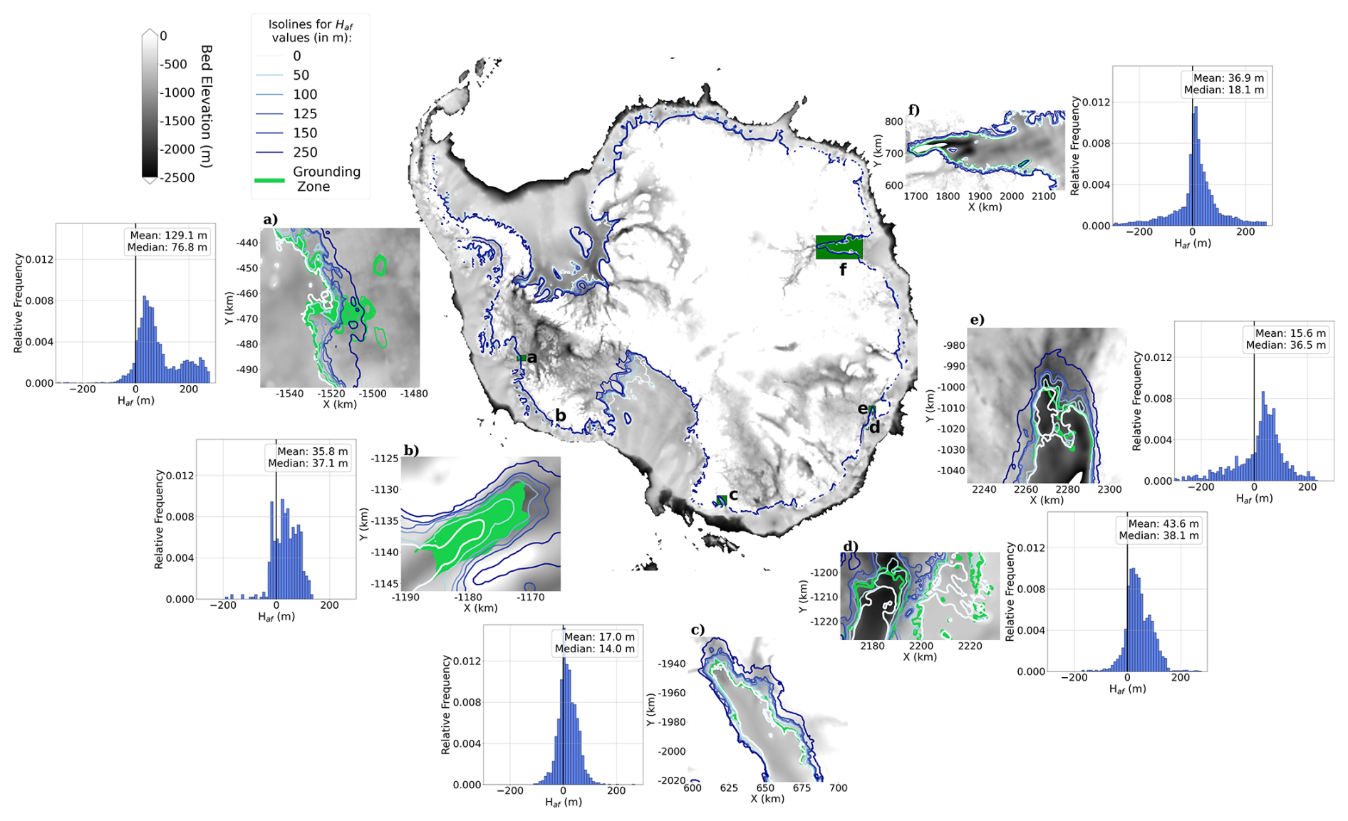
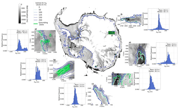
Figure 2 Observational estimates of the GZ for different regions compared with isolines of thickness above flotation. Rectangles with letters (a–f) delimit the extension of the different regions of the insets, for which the observational GZ obtained through DInSAR from different studies is shown in green: (a) Thwaites Glacier (Rignot et al., 2024), (b) Berry Glacier (Chen et al., 2025), (c) Rennick Glacier (Ross et al., 2025), (d) Moscow University Glacier (Ross et al., 2025), (e) Totten Glacier (Ross et al., 2025) and (f) Amery Ice Shelf (Zhu et al., 2025). The isolines of thickness above flotation, H_af, are calculated from the Bedmap3 dataset (Pritchard et al., 2025) with a resolution of 500 m. Grayscale shading shows the bedrock topography. Next to each panel, histograms of the H_af (m) values are shown corresponding to the data points contained within the GZ. Mean and median values are indicated in each panel.

Starting from these spin-ups we carried out projections of the AIS from 2015 to 3000. Until 2300, we used the output of the CCSM4 and CESM2-WACCM General Circulation Models (GCMs) under the RCP8.5 and SSP5-8.5 scenarios, respectively, which provide annual SMB anomalies with respect to the reference year (here 2015) based on the precipitation, runoff, evaporation, and sublimation calculated by the GCM. These anomalies are added to the reference SMB used during the spin-up. The oceanic annual mean thermal forcing is derived from the GCM output as described by Jourdain et al. (2020), and also added to the climatology used during the spin-up. From 2300 to 3000 the forcing is kept constant and equal to the average of the period 2291–2300. This corresponds to a strong oceanic thermal forcing, reaching up to 8 K by the end of the period in CESM2-WACCM, and up to 6 K in CCSM4 (Fig. S4).

We assess the sensitivity of the projected Antarctic SLC to the extent of the tidal water intrusion by varying H_t within the specified range (see below) at 25 m intervals. The case of H_t=0 corresponds to our default model setup when tides are not considered, which serves as a basis for understanding the impact of including water intrusions into the GZ. A control run with no anomaly forcing is also carried out for each H_t value.

3 Results

3.1 Assessment of the parameter H_t

To estimate a reasonable range for the parameter value H_t, we use recent observations of the GZ for several regions obtained through differential radar interferometry (DInSAR) in the Amery Ice Shelf (Chen et al., 2023; Zhu et al., 2025), the Thwaites Glacier (Rignot et al., 2024), Berry Glacier (Chen et al., 2025); and three glaciers within the EAIS: Totten Glacier, Rennick Glacier, and Moscow University Ice Shelf (Ross et al., 2025). In Fig. 2, these regions are shown with isolines of H_af overlain as determined from the Bedmap3 ice and bedrock topography (Pritchard et al., 2025). In all cases, the observed GZ is found to lie well within H_af < 250 m. The different datasets have a distribution that is clearly skewed towards positive values (Table B1), suggesting that GZ extents are well above zero, typically in the range H_t = [15,130]  m (Fig. 2). Based on the deduced values for H_t in the observations, we define the extended range H_t = [0,150]  m for testing the PMPT parameterization, and we set H_t=0 as the reference case.

An exception is the Amery Ice Shelf (Figs. 2f and S5), where our parameterization fails to represent the observed GZ regardless of the H_t value. We attribute this mismatch to a likely bias in the topography dataset where the bedrock uncertainty reaches more than 250 m (Pritchard et al., 2025). Therefore, leaving aside this case, our parameterization broadly captures the observed GZs for which DInSAR data and reasonably good estimates of the bedrock topography are available. We have also made a similar comparison for two Greenland glaciers (Fig. S6) that supports our approach: Petermann Glacier (Ciracì et al., 2023) and Jakobshavn Isbrae (Kim et al., 2024). This illustrates that the parameterization can be applied to any ice sheet, and comparisons across different grounding zones and isolines in Greenland may provide a way to evaluate its applicability. However, we note that Greenland has a stronger seasonality and our approach does not assume any subglacial environment conditions.

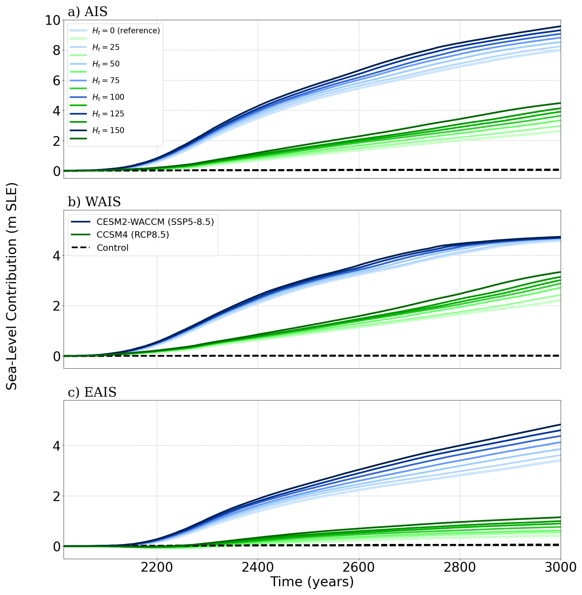
Figure 3 SLC relative to 2015 (m  SLE) for the different values of H_t (in m) used. In (a) for the whole AIS, in (b) for the WAIS, and in (c) for the EAIS. Dashed lines represent the control simulations corresponding to the different values of H_t, overlapping as variations are very small during the simulation period.

3.2 Projections of sea-level contribution

Figure 3 shows the projected SLC of the AIS for the different values of the tidal intrusion parameter for the two different GCMs with high-emission scenarios used, CESM2-WACCM (SSP5-8.5) and CCSM4 (RCP8.5). The total SLC clearly increases with increasing H_t. Differences are already apparent in 2100, although their absolute magnitude remains small (∼ 0.04 m  SLE). These differences highlight the vulnerability of the AIS to tidal intrusions over these timescales (Fig. S7).

For CESM2-WACCM, the SLC progressively grows until 2300 where it ranges from 2.1 to 2.6 m  SLE for the estimated lower (H_t = 0 m) and higher (H_t=150 m) limits, respectively (Table B2). Meanwhile, for CCSM4, it varies betweeen 0.3 and 0.6 m  SLE (Table B3).

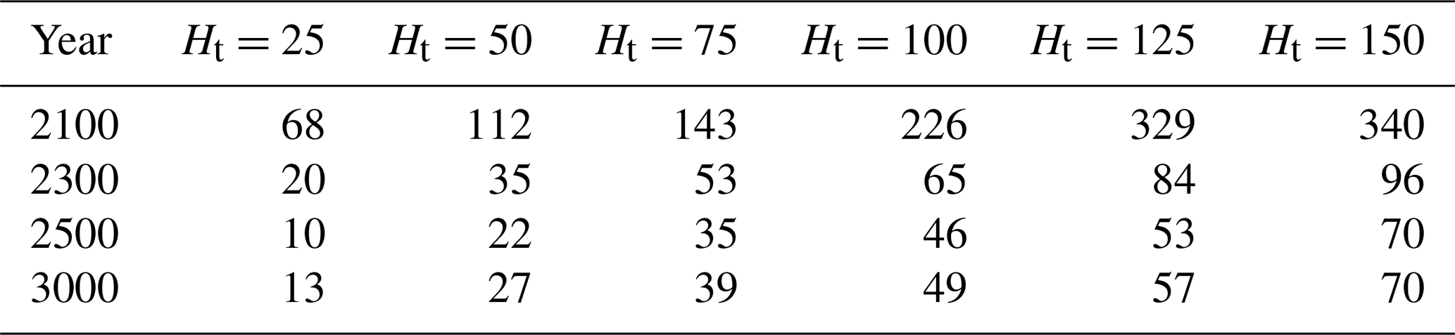
While for CCSM4 the SLC increases linearly throughout the whole period, for CESM2-WACCM, it starts to increase more slowly after 2300. By 3000, it ranges between 8.0 and 9.6 m  SLE, for the lower and higher H_t limits, respectively. The spread, therefore, grows over time, reaching roughly 1.6 m  SLE (or 20 % relative to the reference case H_t=0) by the end of the simulation. For CCSM4, the SLC range has lower values, between 2.6 and 4.5 m  SLE, with the spread reaching 1.9 m  SLE (70 % compared to the reference case H_t=0).

In CESM2-WACCM, the isolated SLC stemming from the WAIS follows a similar increasing evolution (Fig. 3b). At 2300, it yields about 1.4 m  SLE. At 3000, however, it shows no sensitivity to tidal intrusion, reaching about 4.6 m  SLE for all H_t values. The reason for this behaviour is essentially the saturation in mass loss in the region, since by this point the WAIS has collapsed entirely. The East-Antarctic SLC in contrast shows a very large spread. By 2300, its contribution ranges between 0.8 and 1.1 m  SLE and, by 3000, between 3.4 and 4.8 m  SLE, in both cases for the lower and higher tidal-intrusion estimated limits, respectively (Table B2). The SLC increase attributable exclusively to the inclusion of tidal melt varies between 3 % and 20 % for H_t = 25 m and H_t = 150 m, respectively, relative to the reference case where H_t = 0 m (Table B4).

In contrast, using CCSM4, the WAIS does not collapse until much later for all H_t values, contributing between 2.2 and 3.3 m  SLE at 3000 for the abovementioned limits (Table B3). In the EAIS, the total contribution is even lower, being below 1.1 m  SLE for all cases. The control runs show negligible trends, varying less than 12 cm  SLE over 1000 years in all cases (Fig. 3).

3.3 Spatial variations in response to tidal intrusions

The value of H_t affects the SLC through its effect on basal melting within the GZ. Basal melting is the weighted sum of the contributions for grounded and floating ice (Eq. 3), with the latter typically much larger in magnitude. Inspecting cumulative basal melting in the first decade allows us to identify the effect of enhanced intrusion in basal melting within the GZ before the forcing has caused a significant retreat or significantly affected the ice flow and thereby basal melting due to frictional heat. Increasing H_t leads to larger basal melting as a result of larger intrusion (Fig. S8), which is most clearly seen in the WAIS, notably in the Ronne–Filchner and Ross ice shelves, and in the Pine Island and Thwaites Glaciers, due to the higher thermal forcing in these regions at the beginning of the simulations (Fig. A1 in Juarez-Martinez et al., 2024) and the thermal forcing correction at the end of the spin-up. The intrusion length therefore controls the amount and extent of basal melting within the GZ at early stages.

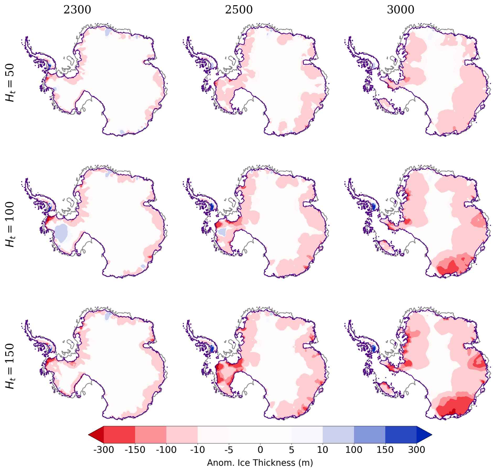
Figure 4 Ice thickness anomalies (m) for the different values of H_t at different timesteps with respect to the case where H_t = 0 m for the experiments with CESM2-WACCM (SSP5-8.5). The gray and purple lines represent the initial and evolving GL, respectively (defined as H_af=0).

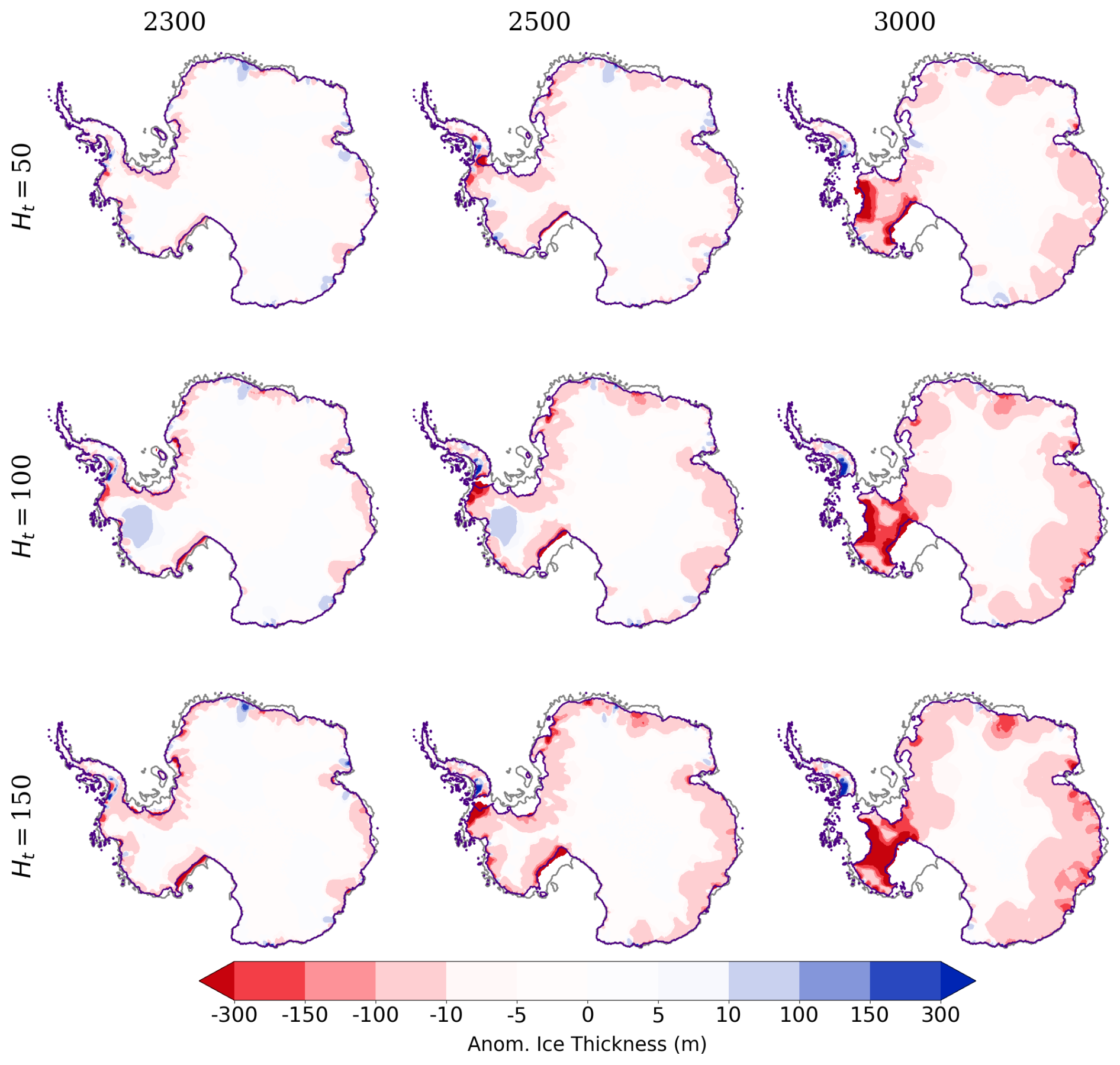
Figure 5 Same as Fig. 4 but for the experiments with CCSM4 (RCP8.5).

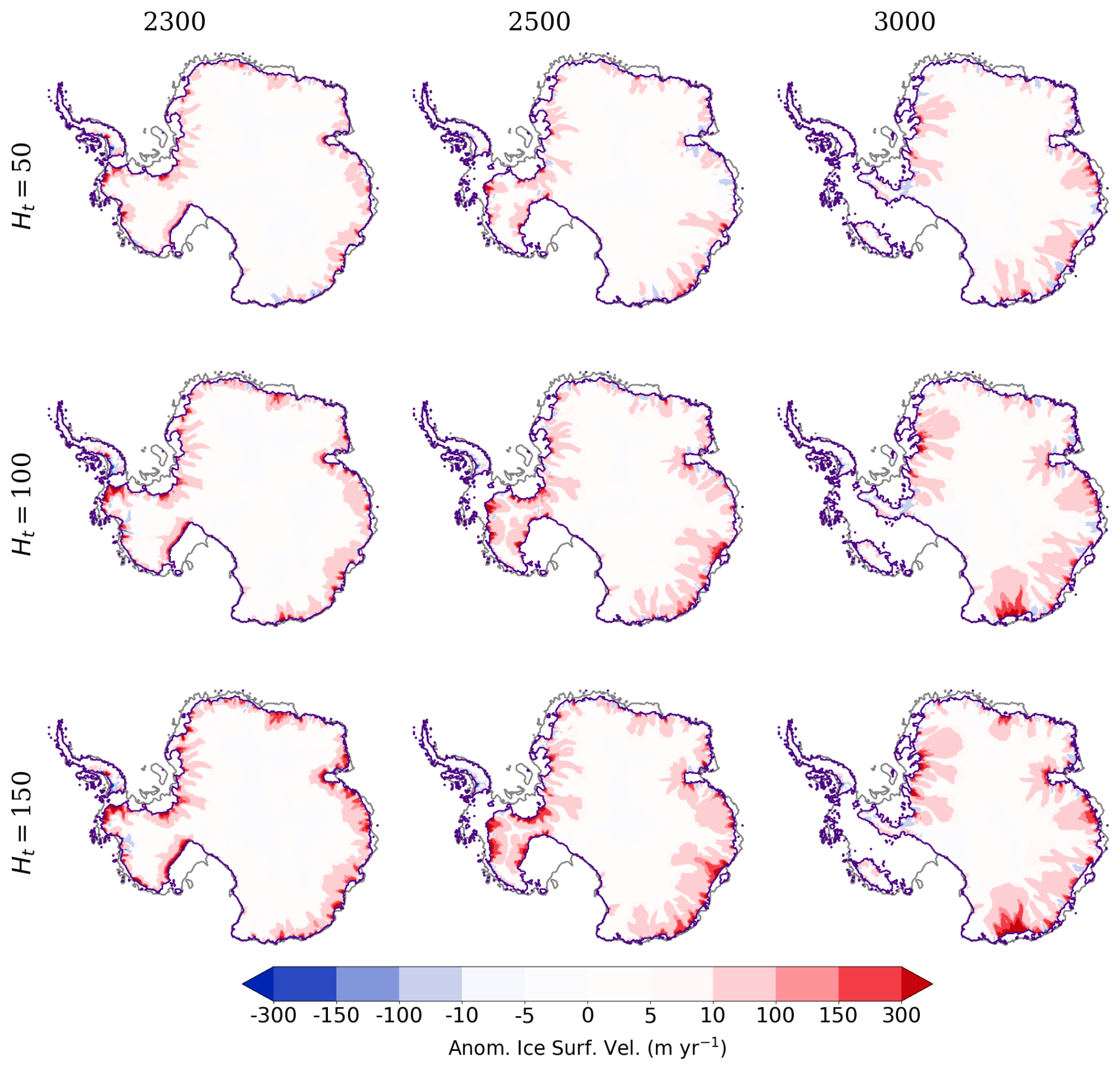
Figure 6 Ice surface velocity anomalies (m yr⁻¹) for the different values of at different timesteps with respect to the case where H_t = 0 m for the experiments with CESM2-WACCM (SSP5-8.5). The gray and purple lines represent the initial and evolving GL, respectively (defined as H_af=0).

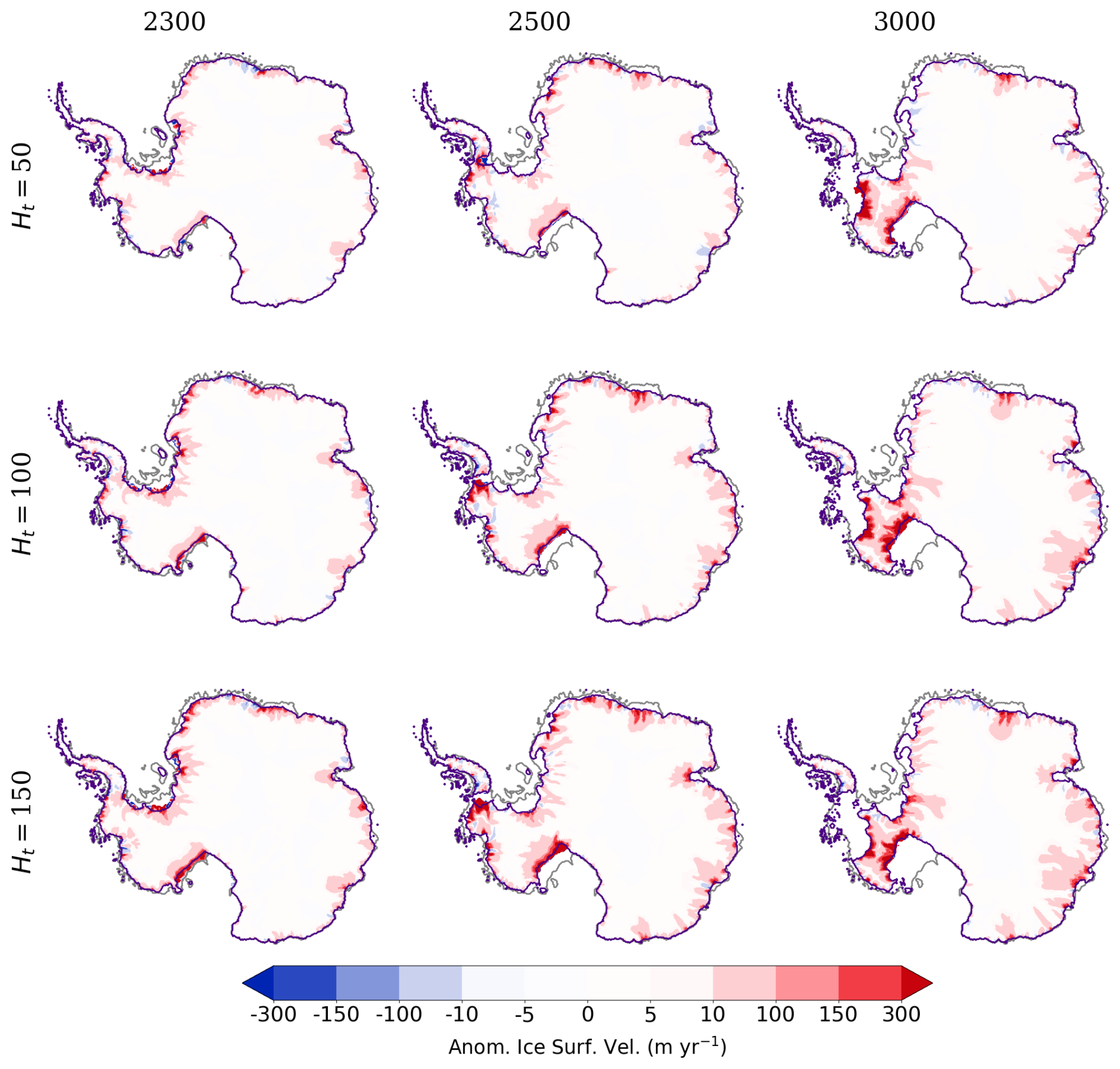
Figure 7 Same as Fig. 6 but for the experiments with CCSM4 (RCP8.5).

The enhanced basal melting contributes to increased discharge and further ice thinning (Figs. 4 and 5), producing an acceleration of ice streams and increasing ice surface velocities (Figs. 6 and 7). For CESM2-WACCM, although the imposed forcing (Fig. S9) is substantial and contributes to the large response of the system, the value of H_t is the primary factor controlling the temporal evolution of spatial anomalies in ice thickness and ice surface velocities relative to the reference case (H_t=0). By 2300, most of the ice-mass loss takes place in the WAIS, where the basal melting is the largest. The Antarctic Peninsula almost becomes detached from the rest of the ice sheet, and the GZ shows a general retreat towards the interior, notably at the western limit of the Ross Ice Shelf. The GZ retreat enhances the acceleration of ice streams and, over time, allows anomalies to extend hundreds of kilometres inland with respect to the reference case. In CCSM4, ice loss changes are considerably smaller and mostly limited to the Ronne–Filchner Ice Shelf, and incipient in the Ross Ice Shelf, notably for H_t = 150 m.

In the eastern part, the Recovery basin also shows substantial grounding-line retreat, ice-stream acceleration, and ice loss for both forcings. In the EAIS, the retreat of the GZ is much more limited in comparison, although the basal melting anomalies in both areas are, however, comparable regardless of the forcing (Figs. S10 and S11). Accordingly, the ice-thickness and velocity anomalies clearly increase with increasing H_t, independently of the forcing. Ice only increases in a small region near the Amundsen Sea in response to lower velocities, but these anomalies revert their sign as the simulation progresses in time, and ice loss both in the WAIS and the EAIS intensifies and spreads farther into the ice-sheet interior. Again, the retreat of the GZ is faster with increasing H_t values, in response to the increase of basal melting anomalies. By 2500, it is predominantly concentrated in the Amundsen Sea and the Ross Ice Shelf. By 3000, the high oceanic thermal forcing of CESM2-WACCM (Fig. S9) eventually leads to an almost complete collapse of the WAIS for all H_t values. This explains the almost zero spread in the West-Antarctic SLC for CESM2-WACCM shown in Fig. 3b. In the EAIS, George V and Wilkes Land now show a larger ice loss than the Recovery Basin due to their stronger marine character (Fig. S9). Meanwhile, for CCSM4, these ice shelves show substantial ice-mass loss by 2500 but, a total collapse of the WAIS is not reached by year 3000.

4 Discussion

Observational evidence of significant tidal intrusions upstream of the Antarctic GL challenges the paradigm of strongly limited basal melting beyond the GL, prevalent in current modelling of the AIS. Tidal intrusions may significantly influence GL behaviour and ice dynamics, in particular, the future evolution of the AIS. These processes, however, have not been explicitly accounted for in large-scale ice-sheet projections, including modelling frameworks such as ISMIP6.

Rignot et al. (2024) suggested that models with GZ lengths of several kilometres should produce higher projections of glacier loss, with SLC increasing by a factor of two for very high melting. In the long term, our results show a general trend of an increase in SLC with increasing tidal penetration, approximately by 20 %–70 % depending on the forcing used.

For CESM2-WACCM, the sensitivity of the SLC is entirely due to the spread in the EAIS contribution. The WAIS response in this scenario and GCM model is not sensitive to the strength of tidal penetration at the end of the simulation period. This is a consequence of the strong forcing in CESM2-WACCM under SSP5-8.5, which causes its collapse for all H_t values, yielding an SLC of around 4.6 m  SLE by year 3000. However, H_t controls the timing of this collapse. For instance, for H_t = 0 m, the level of 4 m  SLE is reached at year 2778, while with H_t = 150 m already in the year 2671. Specifically for Thwaites, the simulation with H_t = 150 m shows a collapse nearly 100 years earlier than the simulation with H_t = 0 m. Robel et al. (2022) reported similar results when GZs are represented, finding that complete deglaciation of Thwaites occurs up to 200 years earlier than in simulations without GZ representation. For CCSM4, with a milder forcing, the spread in the sensivity is due both to the WAIS and the EAIS responses.

Before 2100, the sensitivity with respect to the strength of tidal penetration is limited. Therefore, it is unclear at this point whether our parameterization would be able to account for a larger current ice-mass loss. Investigating this issue would require mimicking the exact oceanic forcing during the recent decades, including its variability, which is outside the scope of our analysis.

The simulated mass gain until year 2300 in the adjacent areas of the Amundsen Sea Embayment (Figs. 4 and 5) may appear counterintuitive, given the region's well-known sensitivity to ocean forcing. This is explained by the difference in ice thickness at the beginning of the simulations which happens to give H_t=0 an underestimation in ice thickness with respect to other values of H_t, due to slightly higher temperatures at the end of the spin-up. Despite the optimization, which aims to match the observed ice thickness, our spin-up includes 4000 years when the two inverted parameters are held constant and thus some drift in the model state away from observations can occur. This suggests that an even more realistic initialization (e.g., involving a more accurate ocean temperature target) could improve small aspects of the projections. Nevertheless, this mass gain is relative to H_t=0, small and transient, and does not contradict the long-term vulnerability of the region.

Our parameterization for basal melting goes in line with the suggestion of Robel et al. (2022) of dynamically calculating the GZ length. In our case, this length solely depends on the bed and ice thickness slopes. Chen et al. (2023) and Zhu et al. (2025) showed that the length of the GZ decreases with increasing slopes of the ice thickness, and most notably the bedrock, following almost an exponential law. Our parameterization captures this to a certain extent through its dependency on these topographical features. Ross et al. (2025) further showed a linear dependency with ice velocity on regions with thicker glaciers and faster ice flows, with the elasticity of ice playing a key role in the physical process.

Our approach is simple to understand and investigate, easy to implement, and does not involve any additional computational costs. However, it does not take into account layered seawater intrusion that can take place when subglacial water is discharged to the ocean close to the GZ (MacGregor et al., 2011; Horgan et al., 2013; Milillo et al., 2019; Wilson et al., 2020; Robel et al., 2022). Including this effect would require the inclusion of a comprehensive subglacial hydrology module, which is absent in most ice-sheet models and represents a large source of uncertainty (Robel et al., 2022; Kazmierczak et al., 2024). A more sophisticated treatment of seawater intrusion in ice-sheet models would also include its dependency on the local bed type (hard or soft). However, the extent of soft and hard beds below the Greenland and Antarctic ice sheets remains somewhat unknown, not only due to a lack of observations but also because of a still improvable modelling of sliding and hydrology.

We have assessed the parameter controlling the length of intrusion using GZ extensions as diagnosed from DInSAR in AIS glaciers, such as Amery (Chen et al., 2023; Zhu et al., 2025) and Thwaites (Rignot et al., 2024) in Antarctica. We have also compared this approach in Greenland glaciers such as Petermann Glacier (Ciracì et al., 2023) and Jakobshavn Isbrae (Kim et al., 2024). We have attempted to include as much observational evidence as possible. As new data might appear in other glaciers, it should be possible to further test this parameterization in the future. We have imposed a spatially constant value of H_t everywhere and tested the overall impact. However, it would also be possible to compare different values of H_t for different regions.

Tidally controlled migrations of the GL occur on very short timescales of hours to days that are not resolved here. High-resolution studies solving the tidal cycle indicate that the resulting basal melting distribution along the GZ is highly asymmetric, and that submarine melting is limited to around 72 % of its length, such the case of Petermann Glacier in Greenland (Gadi et al., 2023). Additional studies should provide clues as to how to translate high-frequency forcing into the effective basal melting required by ice-sheet models.

Regarding our experimental setup, model resolution is a key parameter. This is especially true at coarse resolutions, such as the 16 km grid used here, that do not fully capture the dynamics of ice flow across the GL, even when subgrid or parameterization schemes are applied (Williams et al., 2025). To assess the robustness of our results with respect to spatial resolution, we have performed an additional subset of experiments at 8 and 32 km, with the same physical parameters as with 16 km, for CESM2-WACCM. As shown in Fig. S12, the SLC relative to H_t=0 increases as H_t increases, which constitutes the main finding of this study. Quantitatively, the sensitivity with respect to H_t shows some dependence on spatial resolution; however, the overall relationship remains robust across resolutions. Nevertheless, our highest resolution is 8 km which might still be too coarse to properly represent shorter seawater intrusions. In that case our results would underestimate the response to enhanced intrusions.

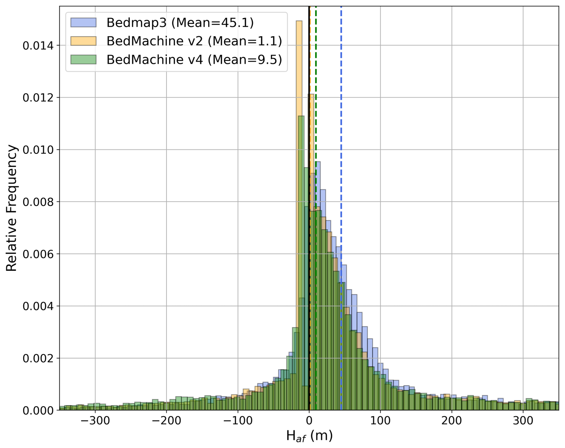
Figure 8 Histograms of H_af (m) for three different topography datasets (Bedmap3, BedMachine v2, and BedMachine v4), using all the GZs regions in Fig. 2. Dashed lines indicate the average value for each topography dataset.

Table 1 Statistical values of the distribution of H_af (in m) values in the GZ for the different topography datasets in Fig. 8: mean, median, standard deviation (σ), first quartile (Q1), third quartile (Q3), fifth percentile (p5) and 95th percentile (p95).

Our model setup contains a number of simplifications. For instance, the DIVA solver used in Yelmo does not solve the full-Stokes flow, implying that not all stress terms are represented, which is important in the GZ. However, DIVA yields better accuracy and stability properties compared to SIA and SSA (Robinson et al., 2022). In our study, the till drainage used following Bueler and van Pelt (2015) typically leads to fully saturated and fully unsaturated regions, as it does not consider any horizontal transport component for the subglacial hydrology (Werder et al., 2013; Sommers et al., 2018; Kazmierczak et al., 2024). Furthermore, ice-shelf melting alters shelf geometry, inducing feedbacks that thereby affect ocean circulation. These feedbacks are absent in the offline framework employed here, which represents a feasible alternative for large-scale applications. Finally, the basal melt parameterization uses a constant value of γ₀. However, it has been noted that a constant value for γ₀ predicts larger melting than a velocity dependent parameter (Burgard et al., 2022). In addition, the intrusions themselves are not explicitly resolved in a geometrical sense, but their influence on ocean-ice interactions is incorporated via the parameterization. This means that the model captures their integrated effect on melt rates without simulating the detailed structure or evolution of individual intrusions.

Regarding parameter sensitivity, the parameterization has thus far been evaluated using the parameter choices specified in Sect. 2. The primary aim of this study is to isolate and assess the behaviour of the new formulation and its dynamical impact on ice-sheet evolution. For this reason, we did not perform a systematic exploration of a broader parameter space, as such an analysis would shift the focus away from evaluating the structure and performance of the parameterization itself. A comprehensive sensitivity study would certainly be valuable and is a natural direction for future work, particularly to better quantify uncertainty and assess robustness across different modelling configurations. However, it is worth noting that the sensitivity to parameter M, which represents the subgrid division of each cell, was tested by increasing its value from M=15 (the default setting) to M=30, with no significant change in SLC, indicating a high degree of convergence (Fig. S13).

Finally, our parameterization is clearly subject to the dataset of the topography used. To show this, we have performed additional analysis with BedMachine v2 (Morlighem et al., 2020) and v4 (Morlighem, 2025) as topography datasets, comparing with the default results using Bedmap3. The BedMachine datasets tend to give lower values of height above flotation on average for all the points in the GZs considered in the study (Fig. 8 and Table 1). However, they also largely demonstrate the same skewed distribution towards positive values of H_af. This can be seen in the superimposed histograms in Fig. 8, which allow us to state that the overall need here is to choose positive values of H_t, although there is substantial uncertainty in the topography used for the comparison with observations for H_t that should be taken into account. Moreover, using BedMachine v2 for the experiments, we can conclude that differences between projections with BedMachine v2 and Bedmap3 at the end of the period are below 4 %. In addition, it should be noted that all these topographic datasets provide a mean representation of bed elevations, based on various interpolation approaches spanning different time scales, while the DInSAR products used to compare with the observed H_t are linked to shorter, more specific time intervals. Consequently, this introduces a limitation in the methodology that needs to be considered.

5 Conclusions

We introduce a new parameterization accounting for submarine melting within the grounding zone, which builds upon the classical partial melting parameterization by explicitly incorporating the effects of tidal intrusion. Tidal intrusions corresponding to regions with ice thickness above flotation of between 15 and 130 m yield the best agreement with observations of present-day grounding zones, indicating this may be a realistic and critical parameter range for future AIS models. This approach reveals that the extent of assumed tidal penetration plays a substantial role in long-term sea-level projections. We assess its impact under two high-emission forcing scenarios (CESM2-WACCM with SSP5-8.5 and CCSM4 with RCP8.5), with substantial differences in terms of oceanic thermal forcing. Our simulations show that deeper tidal intrusion can significantly amplify sea-level rise over a 1000-year timescale, with a total sea-level contribution ranging from 8.0 to 9.6 m  SLE (20 %), for CESM2-WACCM, and between 2.6 and 4.5 m  SLE (70 %) for CCSM4. In CESM2-WACCM, while the WAIS shows a near-total collapse regardless of the tidal penetration, the EAIS introduces substantial uncertainty depending on the strength of tidal intrusion, with spreads exceeding 1.4 m  SLE. For CCSM4, the spread is both observed in the WAIS and the EAIS. In both cases, the transient response of the ice sheet depends strongly on the representation of tidally induced basal melting under the ice sheet.

Appendix A: Theory behind the PMPT parameterization

Robel et al. (2022) describe a generalized theory of the physics behind layered seawater intrusions. They use the Ice Sheet System Model (ISSM) to study the impact of allowing such intrusions in an idealized setting with an imposed intrusion length L. By assuming that the basal melt rate $\dot{m}$ decreases linearly from the GL at x=0 upstream until reaching zero at x=L, basal melt can be determined from this equation:

$$\begin{array}{}\text{(A1)}& \dot{m}={\dot{m}}_{\text{GL}}\left(\mathrm{1}-{\displaystyle \frac{x}{L}}\right)\end{array}$$

where ${\dot{m}}_{\text{GL}}$ is the basal melt rate at the GL and the term $(\mathrm{1}-\frac{x}{L})$ can be thought of to represent the fraction of that location that can be considered floating, w_f as in Eq. (5) above. We seek to transform this equation to represent the floating fraction w_f as a function of the ice thickness above flotation H_af instead of L, since the former quantity is easier to diagnose in complex topographies as it only relies on the bedrock elevation, the ice thickness and sea level, which are all known quantities that are strongly related to L in reality (Robel et al., 2022). Given horizontal coordinates defined such that x=0 at the GL, and x=L at the terminus of a given intrusion, we know that $H_{\text{af}}(x=\mathrm{0})=\mathrm{0}$ at the GL by definition, and we can define $H_{\text{af}}(x=L)=H_{\mathrm{t}}$. With these quantities defined, we can define the gradient of H_af as:

$$\begin{array}{}\text{(A2)}& {\displaystyle \frac{\partial H_{\text{af}}}{\partial x}}={\displaystyle \frac{H_{\mathrm{t}}}{L}}\end{array}$$

In essence, this relationship results from the fact that we relax the condition of allowing basal melting only for H_af<0 (under floating ice, downstream of the grounding-line at H_af=0) by allowing melting also for H_af<H_t (under grounded ice, up to a limit value of H_af=H_t). For a given value of H_t, the length of the region over which we allow basal melting will increase with decreasing gradient of H_af.

Appendix B: Additional tables

Table B1 Statistical values of the distribution of H_af (in m) for the observational datasets in Fig. 2: mean, median, standard deviation (σ), first quartile (Q1), third quartile (Q3), fifth percentile (p5) and 95th percentile (p95).

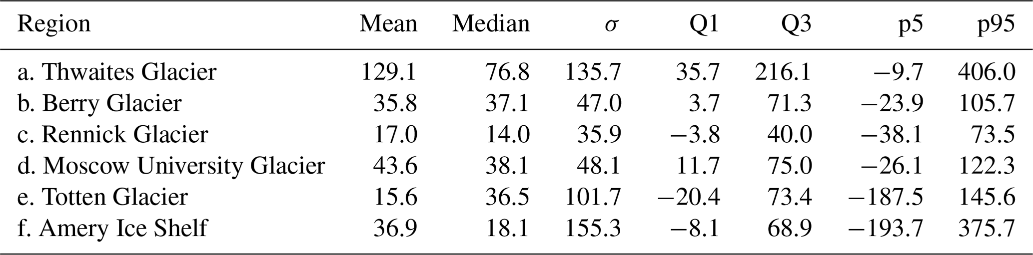
Table B2 Summary of the SLC (m  SLE) at 2100, 2300, 2500 and 3000 from the different AIS sectors at the two extreme values of H_t for CESM2-WACCM.

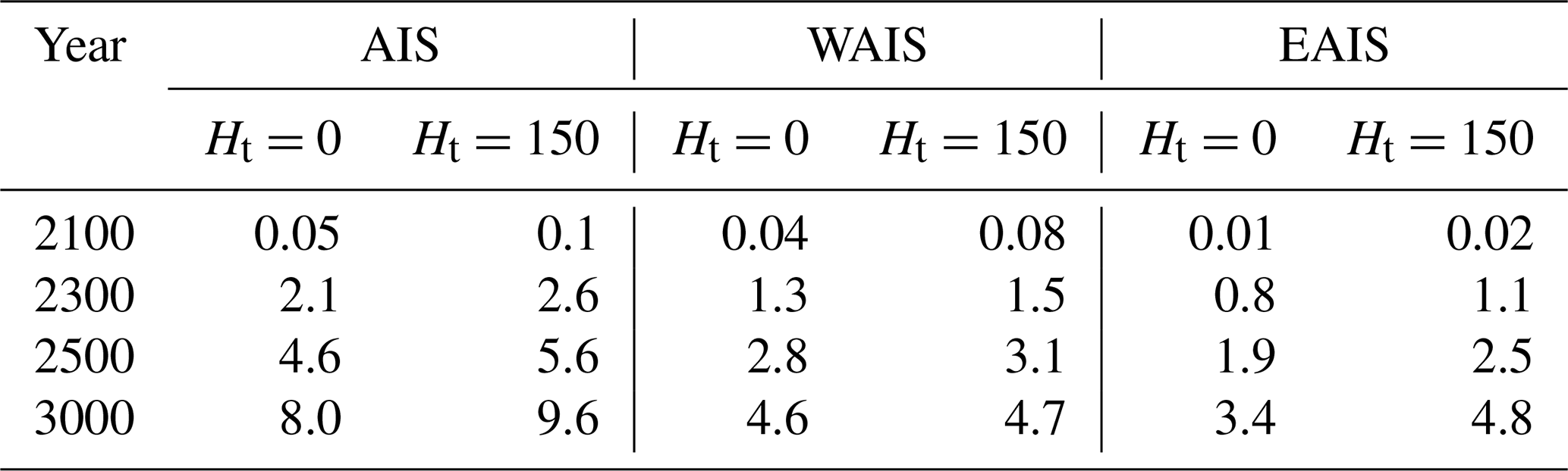
Table B3 Summary of the SLC (m  SLE) at 2100, 2300, 2500 and 3000 from the different AIS sectors at the two extreme values of H_t for CCSM4.

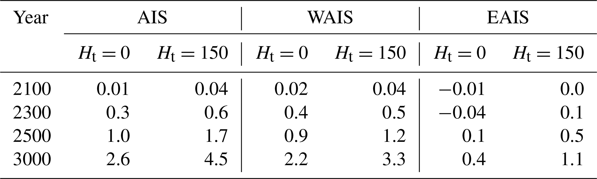
Table B4 Percentage of increase (%) in SLC at 2100, 2300, 2500 and 3000 for the different values of H_t, relative to reference case H_t=0, for CESM2-WACCM.

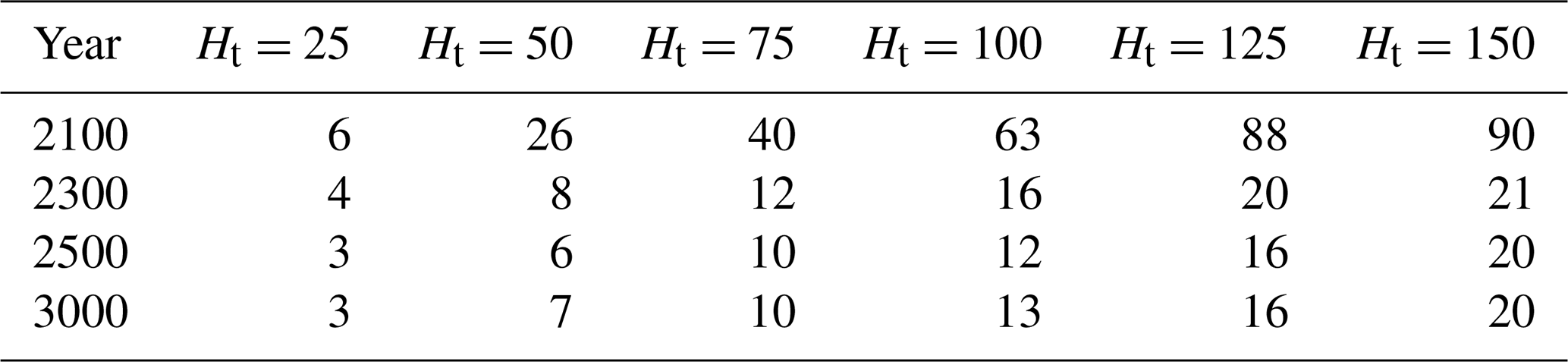
Table B5 Percentage of increase (%) in SLC at 2100, 2300, 2500 and 3000 for the different values of H_t, relative to reference case H_t=0, for CCSM4.