Accelerated lowland thermokarst development revealed by UAS photogrammetric surveys in the Stordalen mire, Abisko, Sweden

Organic matter decomposition in permafrost soils depends on factors such as soil pH, temperature, and redox conditions. Over lowland permafrost soils, these conditions are shaped by microtopography, which evolves with physical degradation, i.e., lowland thermokarst development. A dynamic quantification of lowland thermokarst development – still poorly constrained – is therefore a critical prerequisite for predictive models of permafrost carbon balance in these areas. Here we provide such a quantification, updated for the Stordalen mire in Abisko, Sweden (68°21^′20^′′ N, 19°02^′38^′′ E), which displays a gradient from well-drained stable palsas to inundated fens, which have undergone ground subsidence. We produced RGB orthomosaics and digital surface models from very high resolution (10 cm) unoccupied aircraft system (UAS) photogrammetry as well as a spatially continuous map of soil electrical conductivity (EC) based on electromagnetic induction (EMI) measurements. We classified the land cover following the degradation gradient using a support vector machine algorithm and derived palsa loss rates. Our findings confirm that topography is a key variable for monitoring palsa loss, nearly doubling the overall accuracy of the classification, while slope enabled the identification of early-stage degradation. We show a clear acceleration of degradation for the period 2019–2021, with a decrease in palsa area of 3.3–3.6 % a⁻¹ (% reduction per year relative to the initial palsa areal extent) compared to previous estimates of ∼ 0.3 % a⁻¹ (1970–2000) and ∼ 0.1 % a⁻¹ (2000–2014). EMI data show that this degradation leads to an increase in soil moisture, which in turn likely decreases organic carbon geochemical stability and potentially increases methane emissions. With a palsa loss of 3.3–3.6 % a⁻¹, we estimate accordingly that surface degradation at Stordalen might lead to a pool of 12 × 10³ kg of organic carbon exposed annually within the topsoil (23 cm depth), of which ∼ 25 % is mineral-interacting organic carbon. These results demonstrate that UAS monitoring can robustly quantify rapid thermokarst development that coarser methods miss, and provide a transferable framework for tracking permafrost degradation rates at other lowland sites.

1 Introduction

Arctic air temperature is increasing three to four times faster than the rest of the globe (AMAP, 2021; Rantanen et al., 2022) and we consequently anticipate that the area of near-surface permafrost will decrease by 2 %–66 % for Representative Concentration Pathways (RCP) 2.6 and 30 %–99 % for RCP8.5, by 2100 (Fox-Kemper et al., 2021; Meredith et al., 2019). Arctic and boreal permafrost region soils and sediments store 1460–1600 Gt of organic carbon (OC; Hugelius et al., 2014; Strauss et al., 2021), which could release 3–41 Pg of carbon as CO₂ per 1 °C of global warming by 2100, with high confidence that this will produce a positive feedback and accelerate climate change (Canadell et al., 2021). In particular, northern peatlands (covering 3.7 ± 0.5 × 10⁶ km²; Hugelius et al., 2020), which have historically acted as carbon sinks, are expected to turn into carbon sources, with a projected thaw of permafrost peatlands leading to greenhouse gas (GHG) emissions equivalent to ∼ 1 % of anthropogenic radiative forcing in this century (Hugelius et al., 2020).

As the permafrost thaws, ground ice melts, along with its associated cementing properties, resulting in surface subsidence. This phenomenon is widespread across the Arctic permafrost region, with thaw subsidence rates of up to 2 cm a⁻¹ in areas with low ice content and more than 3 cm a⁻¹ in regions with ice-rich permafrost (Streletskiy et al., 2025). In the particular areas with large amounts of excess ground ice, we often refer to the development of thermokarst landforms (e.g., Heginbottom et al., 2012; Kokelj and Jorgenson, 2013; Webb et al., 2025), which refer to physical degradations of the landscape that occur when the ground subsides or collapses with significant consequences for hydrologic and biogeochemical cycles (e.g., Turetsky et al., 2020; Varner et al., 2022; Vonk et al., 2015). The development of thermokarst landforms is not included in GHG emissions models used by the IPCC, yet they constitute nonlinear processes which are expected to intensify and compromise the feasibility of remaining below air temperatures of 1.5 or 2 °C targeted by the Paris Agreement (Natali et al., 2021). Turetsky et al. (2020) provided a high-level estimate suggesting that GHG emissions across 2.5 million km² of thermokarst landforms could provide an additional and comparable feedback to that of gradual thaw emissions for the entire permafrost region under the SSP5-8.5 scenario (the Shared Socio-economic Pathway (SSP) corresponding to a very high greenhouse gas emissions scenario; Fox-Kemper et al., 2021).

The estimation of GHG emissions from thermokarst landscapes is challenging, as the decomposition of organic matter depends on factors such as the soil pH, temperature and redox conditions (e.g., Arndt et al., 2013; Canfield, 1994; Hemingway et al., 2019; Keil and Mayer, 2014; Lehmann and Kleber, 2015; von Lützow et al., 2008; Li et al., 2023). Redox conditions may change drastically following thermokarst development, such as from oxidizing to reducing conditions after excess ice melts and wetlands form (e.g., Patzner et al., 2020; Turetsky et al., 2020; Varner et al., 2022; Vonk et al., 2015 and references therein). This can be monitored spatially by measuring soil electrical conductivity (EC), which increases with clay content, water content, salinity, organic matter content, temperature and soil density (Doolittle and Brevik, 2014; McNeill, 1980), and is therefore expected to increase as permafrost degrades and wetlands form (e.g., Mollaret et al., 2019 and references therein). Estimation of GHG emissions from thermokarst landscapes can be achieved by calculating cumulative net ecosystem carbon balance (NECB) trajectories from different models of thermokarst landscape succession, directly influenced by the rate of permafrost degradation (Bosiö et al., 2012; Turetsky et al., 2020). Methods for monitoring thermokarst landscape development vary with degradation type and spatial scale (e.g., Barry and Hall-McKim, 2018; Burn and Lewkowicz, 1990; Farquharson et al., 2019; Godin and Fortier, 2012; Heginbottom et al., 2012; Kokelj et al., 2021; Kokelj and Jorgenson, 2013; Lamoureux and Lafrenière, 2009; Lewkowicz, 2007; Lewkowicz and Way, 2019; Olefeldt et al., 2016; Patzner et al., 2020; Vonk et al., 2015). Large-scale disturbances, affecting several (tens of) meters per year, such as thaw slumping (e.g., Kokelj et al., 2017; Lantz and Kokelj, 2008; Nitze et al., 2018; Yang et al., 2023) or lake area losses (e.g., Nitze et al., 2018) can be monitored through satellite remote sensing. For lowland organic-rich landscapes – including peatlands – where thermokarst development leads to the formation of ponds and wetlands, satellite remote sensing is impractical, since landscape deformations can occur on very subtle spatial scales, i.e. only a few tens of centimeters per year, both horizontally and vertically or a few meters of lateral erosion per decade (de la Barreda-Bautista et al., 2022). These constraints make the use of unoccupied aircraft system (UAS) technology appropriate for studying such evolution, as it allows for the collection of imagery with both high temporal and spatial resolutions (e.g., de la Barreda-Bautista et al., 2022).

Permafrost peatlands are characterized by palsas (peat mounds with a frozen core of mineral and organic material, which have relatively small areal extent and a dome-shaped profile) or peat plateaus (usually extensive flat-topped fields of frozen peat elevated above the surrounding peatland). These are both characterized by a thick layer of surface peat that insulates the permafrost. Following permafrost thaw and associated subsidence, these areas can collapse and eventually form open water ponds. Palsa or peat plateau formation and degradation follow a natural cycle, so that developing, mature, degrading and degraded areas – each associated with particular vegetation (e.g., Railton and Sparling, 1973; Zuidhoff and Kolstrup, 2005) and redox conditions (e.g., Varner et al., 2022) – may coexist simultaneously within the same peatland (Payette et al., 2004; Seppälä, 1986; Verdonen et al., 2023; Wang et al., 2023; Zuidhoff and Kolstrup, 2000). With current climate change, however, several field studies have shown a trend towards degradation without the formation of new palsas or peat plateaus (e.g., Borge et al., 2017; Mamet et al., 2017; Olvmo et al., 2020; Payette et al., 2004; Thie, 1974; Verdonen et al., 2023; Wang et al., 2023; Zuidhoff and Kolstrup, 2000). Reported rates of degradation, quantified by comparison with initial palsa areal extent, are extremely variable, i.e., range from 0.1 to 9 % a⁻¹ (% reduction per year) (Borge et al., 2017; Chasmer and Hopkinson, 2017; Christensen et al., 2004; Mamet et al., 2017; Olvmo et al., 2020; Payette et al., 2004; Thie, 1974; Varner et al., 2022; Verdonen et al., 2023; Wang et al., 2023; Zuidhoff and Kolstrup, 2000). This degradation and associated subsidence are most pronounced in the lateral zones of stable permafrost patches (Borge et al., 2017; Mamet et al., 2017; Martin et al., 2021; Olvmo et al., 2020; Renette et al., 2024). Studies further showed that degradation is observed over larger regions, with 55 % of Sweden's largest palsa peatlands currently subsiding (Valman et al., 2024). A few studies suggest an accelerated rate of degradation in more recent years (i.e., from the 1950s to the last decade; de la Barreda-Bautista et al., 2022; Borge et al., 2017; Olvmo et al., 2020), but still require at least 10 years of survey data to enable quantification of palsa loss rates.

In this study, we provide a quantification of the rate of palsa degradation over a shorter timescale, namely between the summers of 2019 and 2021 in the Stordalen mire (Abisko, Sweden) using UAS-based photogrammetric surveys. We combine surface properties (obtained from RGB orthomosaics) with information on micro-topography (relative elevation and slope obtained from digital surface models) to classify the land cover and thereby track palsa degradation over a 2 year period. This enables a short-term quantification of palsa loss rates. We then widen our analysis to cover the years 2014 to 2022 by linking palsa degradation with variation in the areas of open water ponds. Additionally, we use electromagnetic induction (EMI) on a smaller extent to map soil EC and infer contrasts in redox conditions, allowing for comparison with topography, orthophoto-derived vegetation patterns, and classification model results. Ultimately, we use the generated thematic maps to scale up organic carbon stocks, stability and release in the palsa mire. This multi-scale approach aims to improve our understanding of the dynamics of lowland thermokarst development and support future modeling of permafrost-related carbon feedbacks.

2 Methods

2.1 Study area and site description

The Stordalen mire (68°21^′20^′′ N, 19°02^′38^′′ E) is a peatland located approximately 10 km southeast of the town of Abisko in northern Sweden. Permafrost is sporadic in the region and confined to peatlands in valley bottoms and to mountain tops. The mean annual air temperature measured at the Abisko Scientific Research Station (∼ 10 km from Stordalen) has risen by 2.5 °C from 1913 to 2006 and reached 0.6 °C in 2006 (Callaghan et al., 2010). More recently, half-hourly data from the Integrated Carbon Observation System (ICOS) shows that the mean annual air temperature for the period 2014–2022 at the Stordalen mire is 0.8 ± 9.2 °C (mean ± standard deviation), while the mean soil temperature is 2 ± 7 °C at 2 cm and 0 ± 2 °C at 50 cm over the same period (Fig. A1a; ICOS Sweden, 2023). Annual moving averages derived from this same dataset (Fig. A1b) reveal a statistically significant warming trend in soil temperature at 18 of the 20 probes, with rates of up to 0.18 °C a⁻¹ (p-values < 10⁻³; Fig. A1c). Conversely, two probes exhibit slightly cooling trends of approximately 0.01 °C a⁻¹ (p-values < 10⁻³; Fig. A1c). In contrast to the widespread soil warming, air temperature has decreased by 0.17 °C a⁻¹ for the period 2014–2022 (p-value < 10⁻³; ICOS Sweden, 2023). The mean annual accumulated precipitation for 1981–2010 is 332 mm, which is 10 % more than the 1961–1990 normal (ICOS Sweden, 2025).

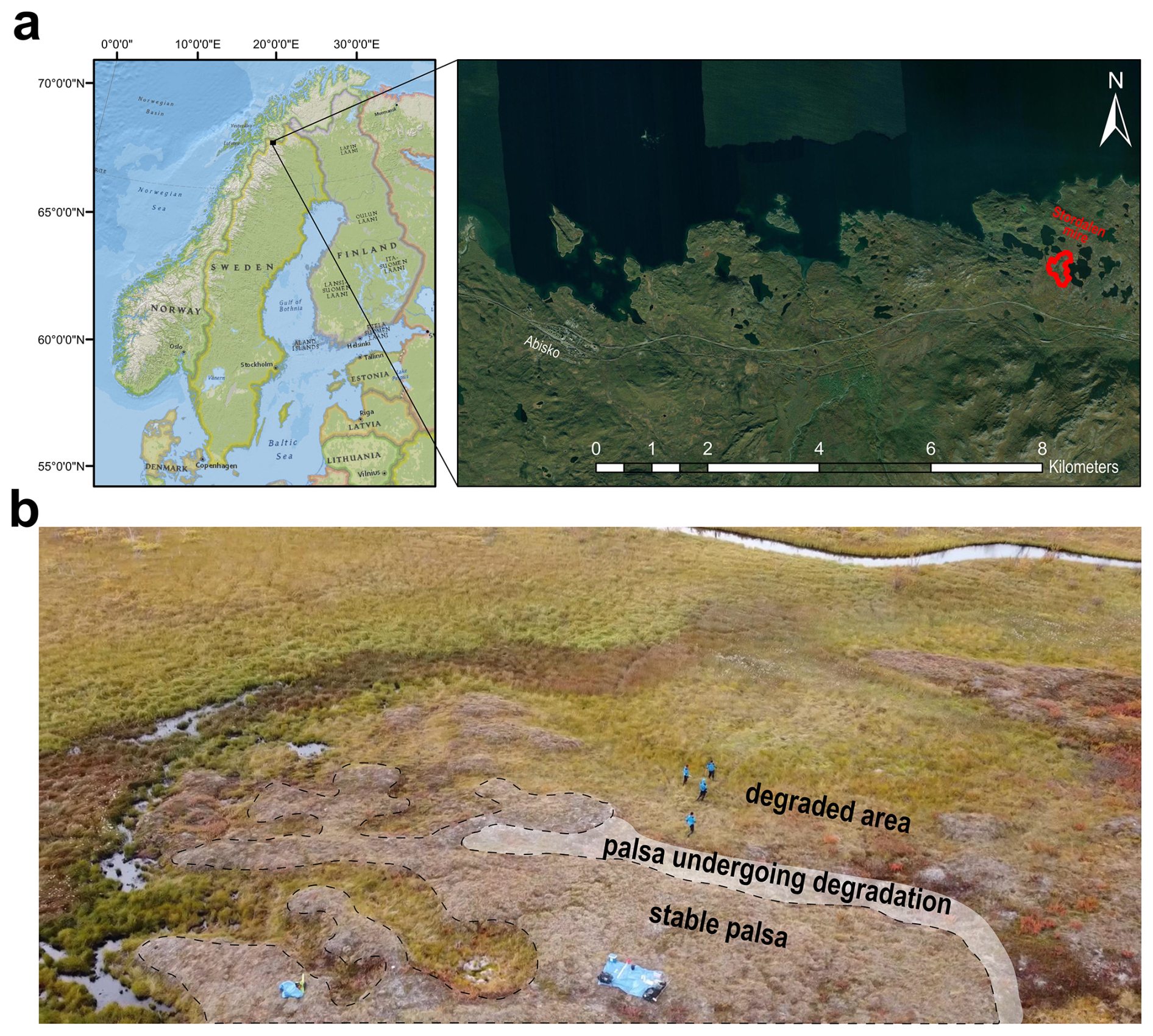
Figure 1 Location and photograph of the degradation gradient studied. (a) Map of the study site at the Stordalen mire, Abisko Sweden. Map created with ArcMap^® 10.8. Basemap sources: National Geographic (© National Geographic et al., 2011) and World Imagery (Esri and Maxar | Powered by Esri, 2022). The projected coordinate system is EPSG: 3006. Delineation adapted from Christensen et al. (2004) in red; (b) Illustration of the degradation gradient showing ground subsidence in the field (photo credit: Maxime Thomas).

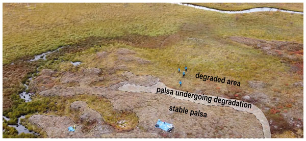
The Stordalen mire consists of three distinct sub-habitats which represent a gradient of permafrost degradation (Figs. 1a, b and A2a). Those three sub-habitats are common to northern wetlands: (i) a well-drained raised palsa with a permafrost core (active layer depth of ∼ 50 cm in 2021), dominated by low-growing ericaceous and woody plants, which is referred to as stable palsa, (ii) palsa undergoing active degradation with fluctuating water table depth and some active thawing, dominated by Eriophorum spp. and Sphagnum spp., which is referred to as a palsa undergoing degradation, and (iii) a fully thawed and inundated fen which has undergone full ground subsidence, indicated by the presence of sedges such as Eriophorum spp. and which is referred to as highly degraded (de la Barreda-Bautista et al., 2022; Siewert, 2018; Sjögersten et al., 2023). The area also includes open water ponds formed by the thawing of permafrost (Burke et al., 2019; Chang et al., 2019b, a; Hodgkins et al., 2014; Johansson et al., 2006; Mondav et al., 2014; Patzner et al., 2020). As an illustration, measurements within an extent of less than 10 m² (Fig. A2a) reveal that the active layer depth varies from 50 cm to more than 200 cm from stable palsa to degraded areas (likely reflecting a complete thaw of permafrost at depth; Fig. A2b) and soil volumetric water content varies accordingly from 20 % to 60 % (Fig. A2c, based on measurements from METER TEROS 12 soil moisture sensors taken on 30 September 2021).

2.2 Photogrammetric survey

To obtain data on surface properties, i.e., vegetation, elevation and ground subsidence, we generated an RGB orthomosaic and a digital surface model of the study site by UAS photogrammetry (UAS: DJI MAVIC 2 PRO L1/L2 PPK). The UAS flight took place on 17 September 2021 at an altitude of 115 m above ground level with a 70 % forward overlap, 63 % side overlap and a camera angle of 90°. The perspective centers of the camera were georeferenced with centimeter-level precision by post-processing RINEX data from a GNSS base station located at Abisko Scientific Research Station (https://swepos.lantmateriet.se, last access: 21 September 2021; reference station 0ABI) using RTKlib v.2.3.4 software (see Zhang et al., 2019 for post-processing kinematic georeferencing). An orthomosaic and a digital surface model (DSM) were derived using Agisoft Metashape professional v1.7.5 from 367 images and led to an initial resolution of 2.66 cm per pixel for the orthomosaic and 5.33 cm per pixel for the DSM.

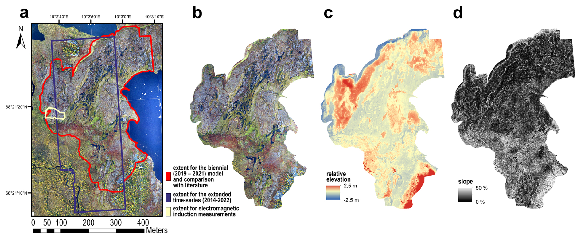
Figure 2 Data processing extents and 2021 input data for classification. (a) Extent of the biennial (2019–2021) model (delineation representing the best compromise between the area covered by our UAS data and the polygon drawn by Christensen et al., 2004) in red, extent for the extended time series (2014–2022) in dark blue and extent used for electrical conductivity measurements in yellow; (b) Orthomosaic composed of red, green and blue bands; (c) Relative elevation after removal of bowl-shape effect (see Fig. A3); (d) slope extracted from the original digital surface model; the projected coordinate system is EPSG: 3006.

2.3 Additional historical data

To assess the temporal evolution of palsa degradation in the Stordalen mire, this study incorporates UAS-acquired data from years other than 2021.

• i.

  We primarily used the 2019 orthomosaic and DSM provided by Siewert and Abisko Scientific Research Station (2020) on the 14 ha extent of the palsa mire (Fig. 2a; delineation representing the best compromise between the area covered by our UAS data and the polygon initially drawn by Christensen et al., 2004). These datasets were collected on 16 August 2019 and have a spatial resolution of ∼ 4 cm for the orthomosaic and ∼ 8 cm for the DSM. For further details on data collection, see de la Barreda-Bautista et al. (2022) and Sjögersten et al. (2023). Together, the 2019 and 2021 datasets provide complementary topographic information and adequate coverage. These were used to develop a classification model for detecting and quantifying palsa degradation between 2019 and 2021.

• ii.

  To capture longer-term trends, we used RGB orthomosaics spanning from 2014 to 2022, although topographic information is unavailable for this dataset. For this analysis, we selected an extent with consistent data availability (Fig. 2a), except for 2020, when data collection was disrupted due to the COVID-19 pandemic. This dataset provides a preliminary estimate of degradation trends from 2014 through 2022. Portions of this data have been previously used in (i) Palace et al. (2018) and Varner et al. (2022) for 2014, (ii) Burke et al. (2019) for 2014 and 2016, and (iii) DelGreco (2018) for the years 2014–2017. Details of these UAS RGB surveys are presented in Table A1.

2.4 Data processing and classification

We carried out the following pre-processing operations on the data: (i) We extracted slopes from DSMs for 2019 and 2021; (ii) We projected all data in the EPSG: 3006 projected coordinate system (SWEREF99 TM); (iii) We performed a co-registration of all raster imagery to ensure the best overlap from one year to the next using the ArcMap^® georeferencing tool using affine transformation with 6 reference points. We chose the 2021 dataset to be the reference for this study; (iv) We then extracted the area of interest (Fig. 2a) by using the ArcMap^® “clip” tool; (v) We resampled all data to a spatial resolution of 10 cm × 10 cm and (vi) removed the bowl-shape effect from elevation data (DSM), to eliminate systematic distortions or artifacts caused by sensor or data processing errors, ensuring accurate inter-annual comparison (Fig. A3).

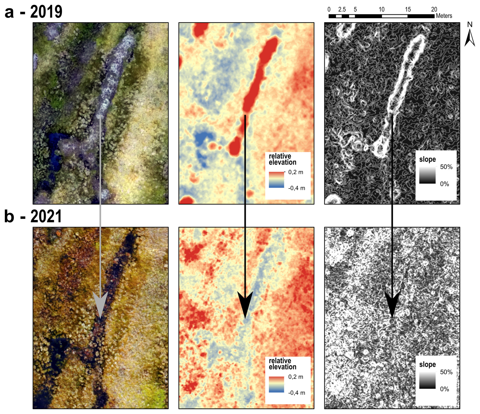
Figure 3 Example of palsa degradation between 2019 and 2021 in the Stordalen mire (Abisko, Sweden). (a) 2019 data from Siewert and Abisko Scientific Research Station (2020); (b) Data from this study. From left to right: orthomosaic, relative elevation and slope. Relative elevation data are corrected after removal of the bowl-shape effect; the projected coordinate system is EPSG: 3006.

For the biennial (2019–2021) model (see Fig. 2a for the spatial extent), we implemented a supervised classification in Python to map four static classes that remain unchanged from 2019 to 2021, and three dynamic classes that represent the evolution of palsa degradation between 2019 and 2021. The static classes include (i) stable palsa surfaces, (ii) areas undergoing or under recent degradation, and (iii) degraded areas, which also include the areas of open water that may not have had permafrost conditions for several decades (e.g., Varner et al., 2022). It should be noted that, for this biennial model (2019–2021), an “open water” class is not considered separately due to the fluctuating height of the water table at the time of the photogrammetric survey. An additional (iv) class called “other” includes outcrops, field equipment, planks, buildings, rocks and trees. The dynamic classes that capture the evolution between 2019 and 2021 include (i) the transition from stable palsa in 2019 to palsa undergoing degradation in 2021, (ii) the transition from stable palsa in 2019 to degraded areas in 2021, and (iii) the transition from palsa undergoing degradation in 2019 to degraded areas in 2021 (Fig. 3).

Table 1 Input data for the classification model. GLCM = Gray Level Co-Occurrence Matrix.

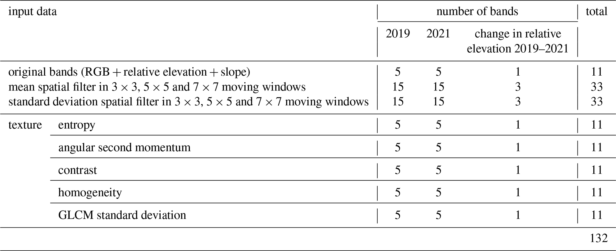
We processed the input data and generated additional data as follows: We first excluded the relative elevation and slope values from the datasets for each of the 2 years (2019 and 2021) that deviate from the mean by more than three times the standard deviation. We then calculated the difference between 2019 and 2021 relative elevation data to obtain the change in relative elevation between the 2 years. We then generated spatial filters from the original bands using pixel windows of varying sizes (Table 1): (i) We calculated the mean pixel values in 3 × 3, 5 × 5 and 7 × 7 moving windows (larger moving windows did not improve the accuracy of the classifications) to reduce the sensitivity of the model to artifacts; (ii) We calculated the standard deviation of pixel values in 3 × 3, 5 × 5 and 7 × 7 moving windows (larger moving windows did not improve the accuracy of the classifications) to distinguish between more homogeneous patches and more heterogeneous patches; (iii) We applied digital image processing techniques to produce texture attributes based on the gray-level co-occurrence matrix (GLCM; e.g., Hall-Beyer, 2017; Haralick, 1979; Haralick et al., 1973) to provide additional morphological information and spatial patterns. The calculated texture attributes include entropy, angular second momentum, contrast, homogeneity and the standard deviation of the GLCM, all applied within a 21 × 21 moving window. These texture indices were calculated on all bands, after standardization. We performed the land cover classifications using a support vector machine (SVM) algorithm. The normalized data served as input for the SVM, with a radial basis function (RBF) as the kernel and the gamma parameter set to automatic. The training points were sampled from polygons drawn as representative of each class (by photointerpretation) and spatially distributed across the mire. The distribution of training points for each class is shown in Table A2 and the data distributions for the training areas are shown in Fig. A4. We performed several runs of the classification with successive additional data inputs to assess the performance of the model (Fig. A5).

As a first post-processing step, we refined the initial predictions with two rules involving the predicted class and the relative elevation difference between 2019 and 2021. Firstly, if a pixel was predicted as belonging to one of the dynamic classes (i.e., representing degradation between 2019 and 2021) and the corresponding relative elevation difference was positive or zero (which therefore does not indicate subsidence), the model re-evaluated the prediction. In this case, the possible identification was limited to one of the static classes that remain unchanged between 2019 and 2021. Conversely, if a pixel was initially assigned to the stable palsa class, and the value of the relative elevation difference was lower than −30 cm (indicating significant subsidence), the model reclassified the pixel by selecting the likeliest identification from the dynamic classes. The reclassification process involved examining the decision scores produced by the model for each sample and selecting the class with the highest decision score from the set of allowed classes. As a second post-processing step, we filtered the classification output with a majority filter of increasing window sizes, from 3 pixel × 3 pixel to 11 pixel × 11 pixel, to reduce noise and enhance classification accuracy. Larger filters did not improve the accuracy of the classifications. Finally, as validation, 1300 points were randomly sampled across the study area and assigned a ground truth class by manual photointerpretation.

To identify representative examples for the evolution of the land cover between 2019 and 2021, we therefore scanned the different data for the two years of measurement and observed the changes in morphology. An example of the transition from stable palsa in 2019 to degraded permafrost in 2021 is presented in Fig. 3.

For the model based on the 2014–2022 UAS time series (see Fig. 2a for the spatial extent), we used data at a spatial resolution of 5 cm × 5 cm and produced one separate classification for each available year, with the following 4 classes: (i) stable palsa surfaces, (ii) degraded areas, (iii) open water and (iv) the class “other”, which includes outcrops, field equipment, planks, buildings, rocks and trees. From the original spectral bands, we used spatial filters on pixel windows of different sizes: (i) the mean of pixel values in 3 × 3, 5 × 5 and 7 × 7 moving windows, (ii) the standard deviation of pixel values in 3 × 3, 5 × 5 and 7 × 7 moving windows, (iii) the GLCM additional texture features entropy, angular second momentum, contrast, homogeneity and the standard deviation of the GLCM in a 21 × 21 moving window. The classifications were performed using an SVM algorithm as for the biennial model.

A validation dataset of 300 points was randomly sampled over the study area and assigned a ground truth class by manual photointerpretation, for each year of data. The predicted surface areas of each class were estimated by pixel counts. We used confusion matrices to correct for misclassification bias in the output maps (Czaplewski and Catts, 1992; Hay, 1988). In the following, all predicted areas presented were corrected using the confusion matrices.

2.5 Performance evaluation of classification models

We used overall accuracy (Eq. 1) as a key metric for assessing the quality of the multiclass model. Additionally, calculations of precision (Eq. 2), recall/detection rate (Eq. 3) and F-score (Eq. 4) were performed to assess the predictive quality of the different classes.

$$\begin{array}{}\text{(1)}& {\displaystyle }& {\displaystyle }\text{overall\hspace{0.17em}\hspace{0.17em}accuracy}\left(\text{OA}\right)={\displaystyle \frac{{\sum }_i{C}_i}{\text{total\hspace{0.17em}\hspace{0.17em}number\hspace{0.17em}\hspace{0.17em}of\hspace{0.17em}\hspace{0.17em}samples}}}\text{(2)}& {\displaystyle }& {\displaystyle }{\text{Precision}}_i={\displaystyle \frac{{\text{TP}}_i}{{\text{TP}}_i+{\text{FP}}_i}}\text{(3)}& {\displaystyle }& {\displaystyle }{\text{Recall}}_i={\displaystyle \frac{{\text{TP}}_i}{{\text{TP}}_i+{\text{FN}}_i}}\text{(4)}& {\displaystyle }& {\displaystyle }{\text{F-score}}_i={\displaystyle \frac{\mathrm{2}\times {\text{Precision}}_i\times {\text{Recall}}_i}{{\text{Precision}}_i+{\text{Recall}}_i}}\end{array}$$

Where i is the class, C_i is the number of correctly classified samples for class i, TP stands for true positive, FP stands for false positive, FN stands for false negative.

2.6 Quantitative analysis of palsa loss rates

To quantify changes in palsa extent, we calculated the average annual rate of reduction of the areas of intact palsa from one year to the next (e.g., Olvmo et al., 2020; Verdonen et al., 2023; Eq. 5). This method assumes that the palsa area decreases annually by a constant percentage applied to the remaining area, analogous to an exponential decay model.

$$\begin{array}{}\text{(5)}& \begin{array}{rl}& \text{average\hspace{0.17em}\hspace{0.17em}annual\hspace{0.17em}\hspace{0.17em}rate\hspace{0.17em}\hspace{0.17em}of\hspace{0.17em}\hspace{0.17em}reduction }\left(\mathrm{\%}{\mathrm{a}}^{-\mathrm{1}}\right)\\ =& \left({\left({\displaystyle \frac{A_{\text{start}}}{A_{\text{end}}}}\right)}^{\frac{\mathrm{1}}{Y_{\text{start}}-Y_{\text{end}}}}-\mathrm{1}\right)\end{array}\end{array}$$

where A_start and A_end are the total areas of palsa at the start year Y_start of the respective period and at the end of it (Y_end). This formulation allows comparison across sites and time intervals of varying length, since the value is normalized to an annual percentage rate.

2.7 Electro-magnetic induction measurements

To measure the soil electrical conductivity along the degradation gradient, we focused on a 0.2 ha sub-area (Fig. 2a) and employed electromagnetic induction (EMI) due to its non-invasive nature, efficiency in covering relatively large areas (several thousand square meters to multiple hectares), and ability to provide continuous conductivity measurements. This approach allows for the identification of spatial heterogeneities in soil properties along the degradation gradient. The instrument used was the EM38, manufactured by Geonics Limited (Ontario, Canada). The EM38 measures soil EC to a depth of 2 m below the sensor, with maximum sensitivity at approximately 30–40 cm (Heil and Schmidhalter, 2017). The EC is estimated using the McNeill model (McNeill, 1980), which is widely applied in EMI surveys. EMI sensors such as the EM38 generate a primary electromagnetic field that induces electrical currents in the ground. These currents generate a secondary electromagnetic field that is measured by the sensor's receiver. Under conditions known as “operating under low induction numbers (LIN)”, the secondary field is proportional to the ground current and is used to calculate soil EC (Doolittle and Brevik, 2014), meaning that the instrument response is linearly related to soil EC. Data collection was conducted on 22 September 2021, by pulling the EM38 on a plastic sledge at a height of a few centimeters above the ground surface. This configuration minimizes soil disturbance while maintaining consistent sensor-to-soil spacing. EMI data and corresponding GNSS positions (acquired by a GNSS BU-353S4 manufactured by GlobalSat) for 1083 points were recorded using a rugged laptop and a custom-made acquisition program. Continuous EC data were interpolated by kriging of the point values after logarithmic transformation, using a combined nugget and exponential model as defined by the fitted covariance function, with a maximum prediction distance of 8 m.

2.8 Use of the classified landscape for scaling up organic carbon stocks

The thematic maps created in this study were used to establish the potential variation in organic carbon stock subsequent to palsa degradation between 2019 and 2021. For each degradation stage (i.e., stable palsa, palsa undergoing degradation and degraded areas), we used the measurements presented in Patzner et al. (2020), which give – for each stage – a characterization of total organic carbon (TOC) content and dithionite/citrate extractable carbon, which is here referred to as mineral-associated organic carbon (MAOC). The study also provides access to the bulk densities and thicknesses associated with the different soil horizons. Using this data, OC stocks ($\frac{{\mathrm{kg}}_{\mathrm{OC}}}{{\mathrm{m}}^{\mathrm{2}}}$) were calculated for each degradation stage (Eq. 6). This assessment was made for a constant mass of mineral matter for each stage, in order to take subsidence and compaction into account (Table B1; Eq. B1). The stock difference between the 2 years (kg_OC) corresponds to the difference between the stocks in 2019 and 2021, weighted by their respective surface areas for each year (Eq. 7). These calculations were carried out for TOC and MAOC. We suggest that this corresponds to a stock of TOC or MAOC that is made vulnerable annually as a result of palsa degradation. The actual timing of OC loss remains unknown.

$$\begin{array}{}\text{(6)}& {\displaystyle }\begin{array}{rl}& \text{OC\hspace{0.17em}\hspace{0.17em}stock}{\left({\displaystyle \frac{{\mathrm{kg}}_{\mathrm{OC}}}{{\mathrm{m}}^{\mathrm{2}}}}\right)}_{j\text{degradation\hspace{0.17em}\hspace{0.17em}stages}}\\ =& \sum _{i\text{horizons}}{\text{bulk\hspace{0.17em}\hspace{0.17em}density}}_i\left({\displaystyle \frac{{\mathrm{kg}}_{\mathrm{soil}}}{{\mathrm{m}}^{\mathrm{3}}}}\right)\\ & \times {\text{thickness}}_i\left(\mathrm{m}\right)\times {\text{OC\hspace{0.17em}\hspace{0.17em}content}}_i\left({\displaystyle \frac{{\mathrm{kg}}_{\mathrm{OC}}}{{\mathrm{kg}}_{\mathrm{soil}}}}\right)\end{array}\text{(7)}& {\displaystyle }\begin{array}{rl}& \mathrm{\Delta }\text{OC\hspace{0.17em}\hspace{0.17em}stock}\left({\mathrm{kg}}_{\mathrm{OC}}\right)\\ =& \sum _{j\text{degradation\hspace{0.17em}\hspace{0.17em}stages}}{\text{OC\hspace{0.17em}\hspace{0.17em}stock}}_j\left({\displaystyle \frac{{\mathrm{kg}}_{\mathrm{OC}}}{{\mathrm{m}}^{\mathrm{2}}}}\right)\\ & \times {\text{surface\hspace{0.17em}\hspace{0.17em}area}}_{j\mathrm{2021}}\left({\mathrm{m}}^{\mathrm{2}}\right)-\sum _{j\text{degradation\hspace{0.17em}\hspace{0.17em}stages}}\\ & \times {\text{OC\hspace{0.17em}\hspace{0.17em}stock}}_j\left({\displaystyle \frac{{\mathrm{kg}}_{\mathrm{OC}}}{{\mathrm{m}}^{\mathrm{2}}}}\right)\times {\text{surface\hspace{0.17em}\hspace{0.17em}area}}_{j\mathrm{2019}}\left({\mathrm{m}}^{\mathrm{2}}\right)\end{array}\end{array}$$

3 Results and discussion

3.1 Information on topography is critical for detecting permafrost degradation

Several runs with successive additional data inputs have been conducted to determine which parameters provide the best classification results for palsa degradation between 2019 and 2021 (see Fig. A5 for model runs). The results reveal that topography is a critical factor for achieving optimal model performance. Classification using only RGB imagery data (i.e. 6 spectral bands but no topography information; run 1) gives an overall accuracy of 41 %. When relative elevation data are added for both years (to reach 8 bands in total; run 2), the overall accuracy increases to 67 %. Other studies have shown that relative elevation is an essential parameter for differentiating otherwise very heterogeneous tundra landscapes, e.g., in permafrost-affected soils of the Lena River Delta (Siewert et al., 2016) or in thermokarst-affected terrain types in the periglacial Lena–Anabar coastal lowland (Grosse et al., 2006). Remarkably, the addition of slope data further improves classification, raising the overall accuracy to 76 % (run 3). The slope additionally doubles the F-scores of both the areas undergoing degradation and the dynamic classes, which makes it particularly valuable for short-term detection of palsa degradation. When the difference in relative elevation between 2019 and 2021 is included (to reach a total of 11 bands; run 4), the overall accuracy reaches 77 %. The relative importance of the different bands is shown on Fig. C1a. For comparison, the use of relative elevation and slope to perform a land cover classification over the Stordalen catchment was also done by Siewert (2018) and resulted in an overall accuracy of 74 %.

By adding data from the mean spatial filters (3 × 3, 5 × 5 and 7 × 7 window sizes; for a total of 44 bands; run 5), the overall accuracy increases to 79 %. Incorporating mean spatial filters over larger windows does not increase classification quality. The addition of standard deviation or texture attributes only improves the classification slightly. Adding standard deviation spatial filters improves the overall accuracy to 80 %, as does the standard deviation of the GLCM, while the addition of angular second momentum, entropy, contrast or homogeneity increases overall accuracy by only 1 %, i.e., to 80.8 %. In the following, we will retain only the “homogeneity” texture parameter (run 6), as it achieves the highest overall accuracy, while the combination of the texture parameters brings it down to 78 %. We believe that GLCM texture attributes contribute little to our model, as topography information already provides a level of morphological information and spatial patterns.

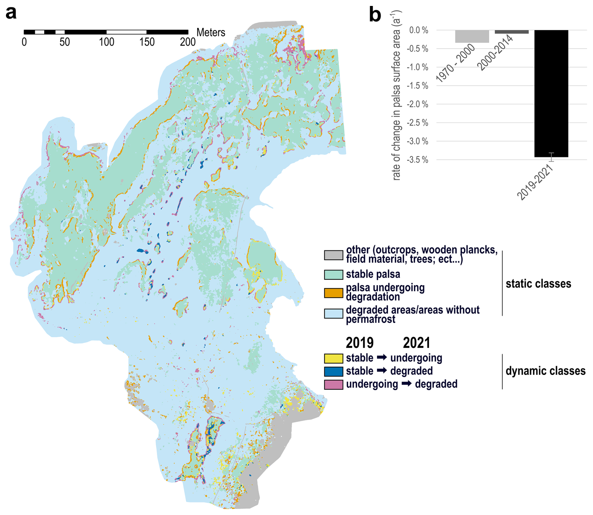
Figure 4 Classification model for the evolution of palsa degradation between 2019 and 2021. This model uses 55 bands as input data, namely (i) 11 bands with original data (3 spectral bands, relative elevation and slope for the years 2019 and 2021 as well as the difference in relative elevation between 2019 and 2021) along with (ii) 3 × 11 bands of the mean spatial filter over windows of increasing size, i.e. 3 × 3, 5 × 5 and 7 × 7, and finally (iii) the 11 bands from the texture attribute “homogeneity”. The classification output was then filtered with a moving window of 11 pixel × 11 pixel. (a) Output landcover map; (b) Rate of change of the stable palsa area for 1970–2000 (Christensen et al., 2004), 2000–2014 (Varner et al., 2022) and 2019–2021 (this study). Rates are expressed as a proportion of the initial palsa areal extent (% reduction per year; Sect. 2.6, Eq. 5). The surface area for 2019–2021 are corrected using the confusion matrix.

Table 2 Confusion matrix for the classification model and precision, recall and F-score for each cover class. This model uses 55 bands as input data, namely (i) 11 bands with original data (3 spectral bands, relative elevation and slope for the years 2019 and 2021 as well as the difference in relative elevation between 2019 and 2021) along with (ii) 3 × 11 bands with spatial filters (mean and standard deviation) over windows of increasing size, i.e. 3 × 3, 5 × 5 and 7 × 7, and finally (iii) the 11 bands from the texture attribute “homogeneity”. The classification output was then filtered with a moving window of 11 pixel × 11 pixel. Bold values represent the diagonal of correct predictions.

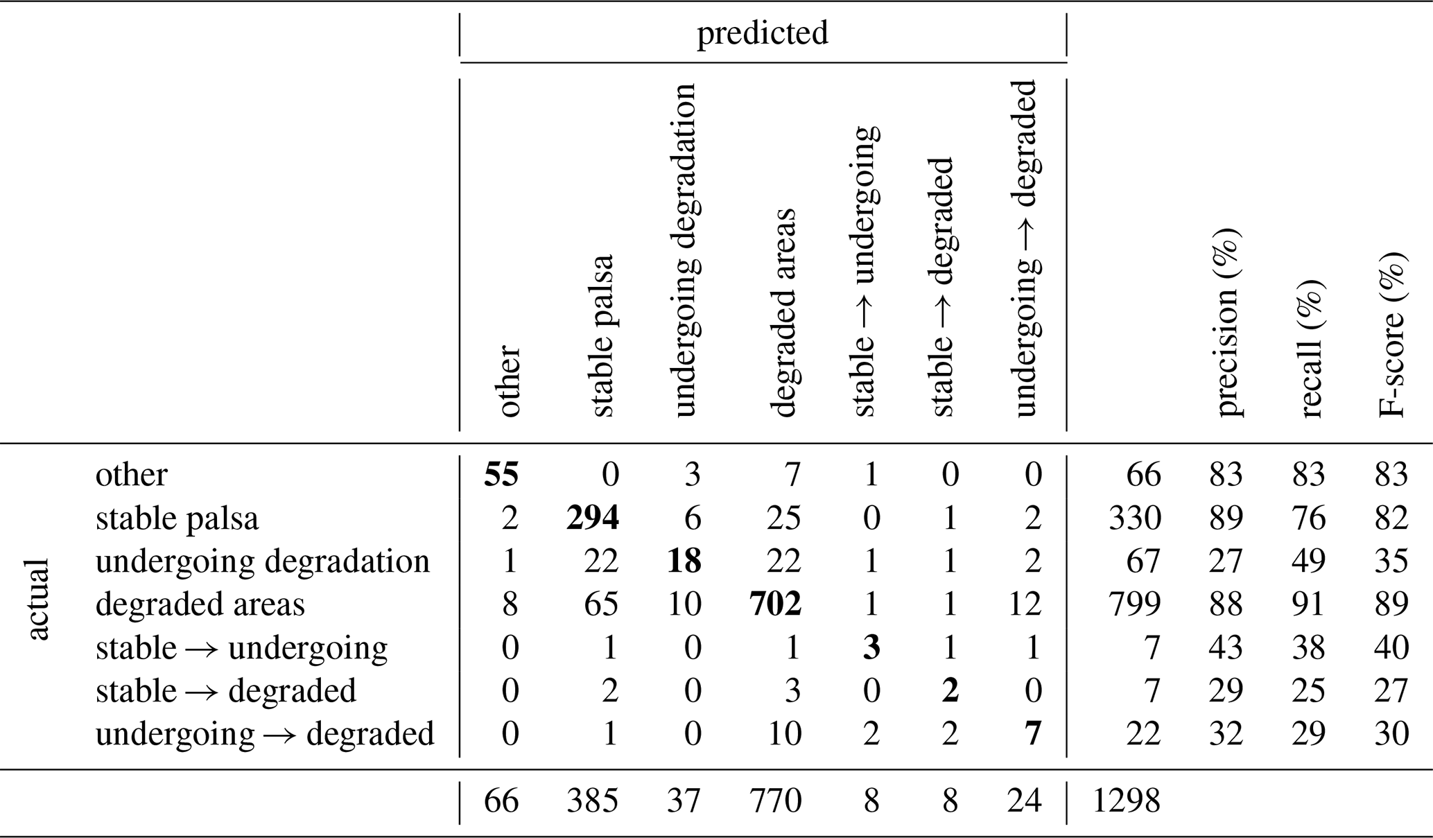
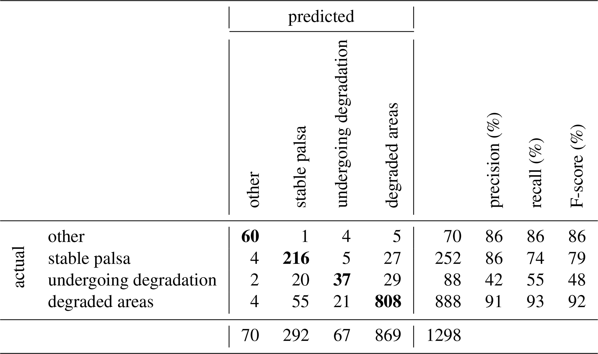
Then, initial predictions were refined using elevation differences and model scores to ensure alignment with domain knowledge (see Sect. 2.4). This procedure affected 0.14 % of the pixels and the overall accuracy improved to 81.3 % (run 7). As a final post-processing step, the classification result was filtered using windows of increasing size up to 11 pixel × 11 pixel, to reduce noise and enhance classification consistency. The improvement of the model's performance for each class is shown in Fig. C1b. These combined operations result in a map with an overall accuracy of 83 % (run 8; Fig. 4a). The best predicted classes are stable palsa, degraded areas and the class “other” with F-scores of 82 %, 89 % and 83 %, respectively. These are followed by palsa undergoing degradation (35 %), the evolution from stable palsa to palsa undergoing degradation (40 %), and the evolution from palsa undergoing degradation to degraded areas (30 %). The class with the poorest performance is the direct transition from stable palsa to degraded areas, with an F-score of 27 % (see confusion matrix in Table 2). The low F-scores for dynamic classes can be attributed primarily to the fact that these classes have intermediate properties between those of the “stable”, “undergoing” and “degraded” classes, making them difficult to differentiate. On the other hand, if we aggregate – for 2019 – the classes “stable → undergoing” and “stable → degraded” together with the “stable” class as well as the “undergoing → degraded” class with the “undergoing” class and vice versa for 2021, we obtain overall accuracies of 84 % and 86 % for 2019 and 2021, respectively. We also obtain significantly improved F-scores, i.e., 49 % and 48 % for the “undergoing degradation” class in 2019 and 2021, respectively (see confusion matrices in Tables C1 and C2).

3.2 Palsa degradation accelerates in the Stordalen mire and can be tracked over 2 years of data

When we compare the rate of palsa degradation for the period 2019–2021 in Stordalen with past studies, we observe a clear acceleration. More specifically, the study by Christensen et al. (2004) reported a rate of disappearance of stable palsa zones averaging 0.3 % a⁻¹ (relative to initial palsa areal extent) between 1970 and 2000, based on vegetation distribution from infrared aerial photographs. Varner et al. (2022) estimated an average palsa loss of 0.1 % a⁻¹between 2000 and 2014, suggesting a deceleration in palsa loss after 2014 relative to the earlier assessment at Stordalen (i.e., 1970–2000; Christensen et al., 2004). In this study, we update these estimates for the period 2019–2021 and we obtain a decrease in palsa surface area of 3.3 to 3.6 % a⁻¹ (Fig. 4b). This suggests that the rate of permafrost degradation in the Stordalen mire is approximately 10 times faster in recent years compared to the 1970–2000 period. Besides, for Stordalen and two other mires in the same valley, de la Barreda-Bautista et al. (2022) mapped lateral erosion of 3.1–9.3 m between 1960 and 2018 with slower rates of 0.03–0.12 m a⁻¹ between 1960 and 2002, and thereafter an acceleration, with the highest rates between 2002 and 2018 with 0.18–0.32 m a⁻¹. This confirms the increasing rate of palsa loss in the mire.

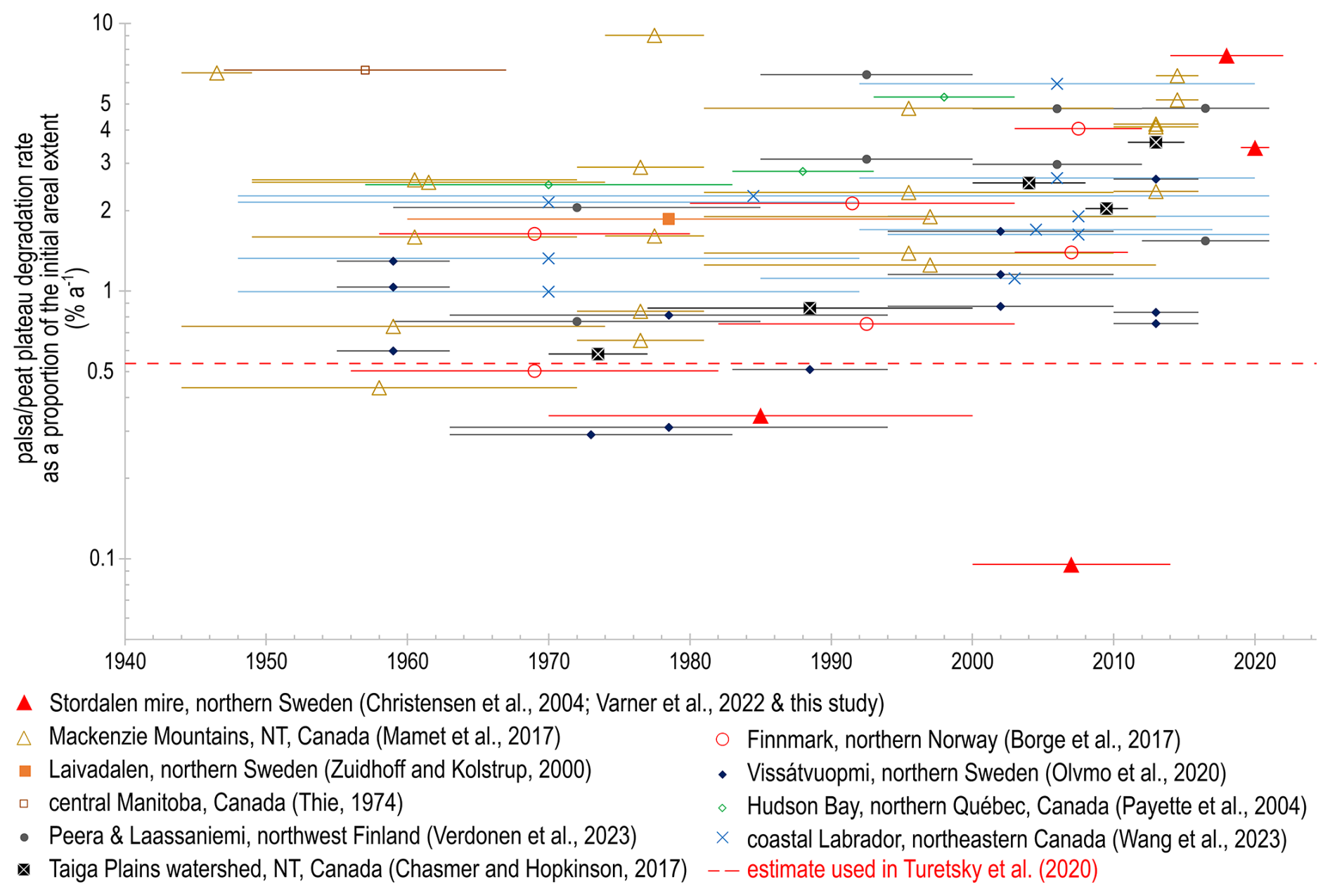
Figure 5 Meta-analysis showing the rates of degradation of palsas/peat plateaus relative to the initial palsa areal extent. Where required, rates reported here were recalculated using Eq. (5) for inter-study comparability.

In Turetsky et al. (2020), the rate of degradation from permafrost peatlands into either active thaw lakes or wetlands was set to be ∼ 0.5 % a⁻¹. Yet this is the only study that attempts – on an Arctic scale – to estimate the changes in greenhouse gas emissions (via cumulative net ecosystem carbon balance estimates) caused by the development of these thermokarst landscapes. According to the published literature and from this study, however, a permafrost peatland's degradation rate of 0.5 % a⁻¹ appears to be a fairly conservative estimate in comparison with other studies across the Arctic, which show extremely variable estimates (0.1–9 % a⁻¹), although most are above 0.5 % a⁻¹ (Fig. 5; Borge et al., 2017; Mamet et al., 2017; Olvmo et al., 2020; Payette et al., 2004; Thie, 1974; Verdonen et al., 2023; Wang et al., 2023; Zuidhoff and Kolstrup, 2000). This meta-analysis (Fig. 5) suggests that palsa degradation is likely to continue, following a non-linear course, probably at a higher rate than today (Borge et al., 2017; Mamet et al., 2017; Olvmo et al., 2020; Renette et al., 2024). Besides, recent modeling studies state that environmental or climate spaces for palsas and peat plateaus are threatened by imminent loss at a circumpolar scale (Fewster et al., 2022; Leppiniemi et al., 2023).

Such assessments of palsa loss rates and development of lowland thermokarst are critical prerequisites for predictive models of permafrost carbon balance from such landscapes. In this study and from available literature, we show that there is still much uncertainty surrounding these estimates beyond local scales, leading to a potential mis-evaluation of the impact of lowland thermokarst on the permafrost carbon balance. From this study, we have shown that biennial data from photogrammetric surveys make it possible to monitor the progression of palsa degradation, although historical data (Christensen et al., 2004; Varner et al., 2022) are essential for assessing the increase in the rate of degradation. In order to monitor this state of degradation, the method proposed here could be extended to cover a large number of study sites of comparable sizes without requiring extensive computing capacity.

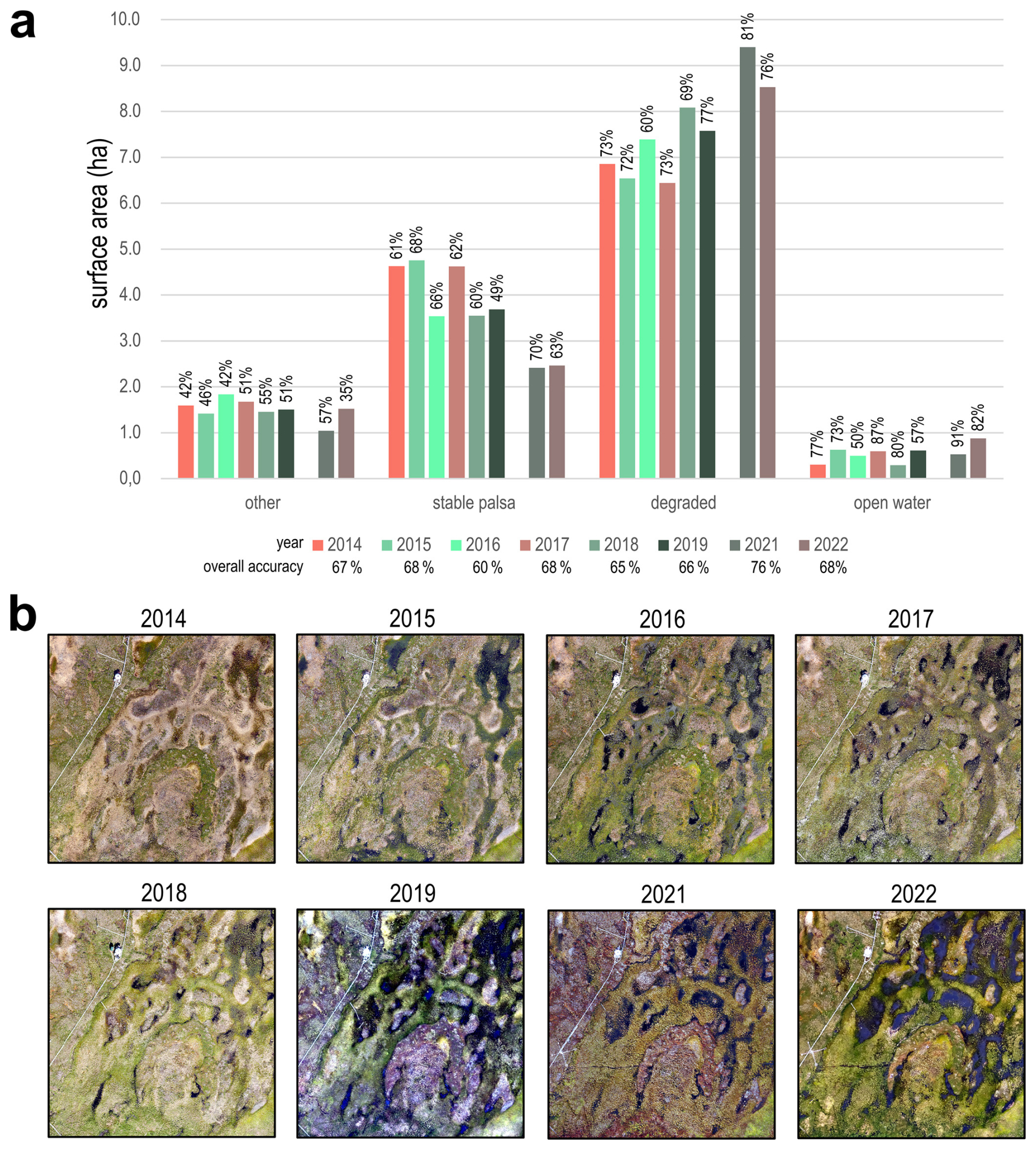
Figure 6 Classification model results based on imagery data spanning from 2014 to 2022. (a) Evolution of the surface areas (corrected using the confusion matrix) of the 4 classes, i.e. (i) stable palsa, (ii) degraded areas (fully thawed fen), (iii) open water and (iv) the class “other”, which includes field equipment, planks, buildings, rocks and trees. Bar colors represent years. Percentages above the bars represent the F-score. The overall accuracy of each of the annual classifications is also shown. (b) Extract (clip) of original data for each available year.

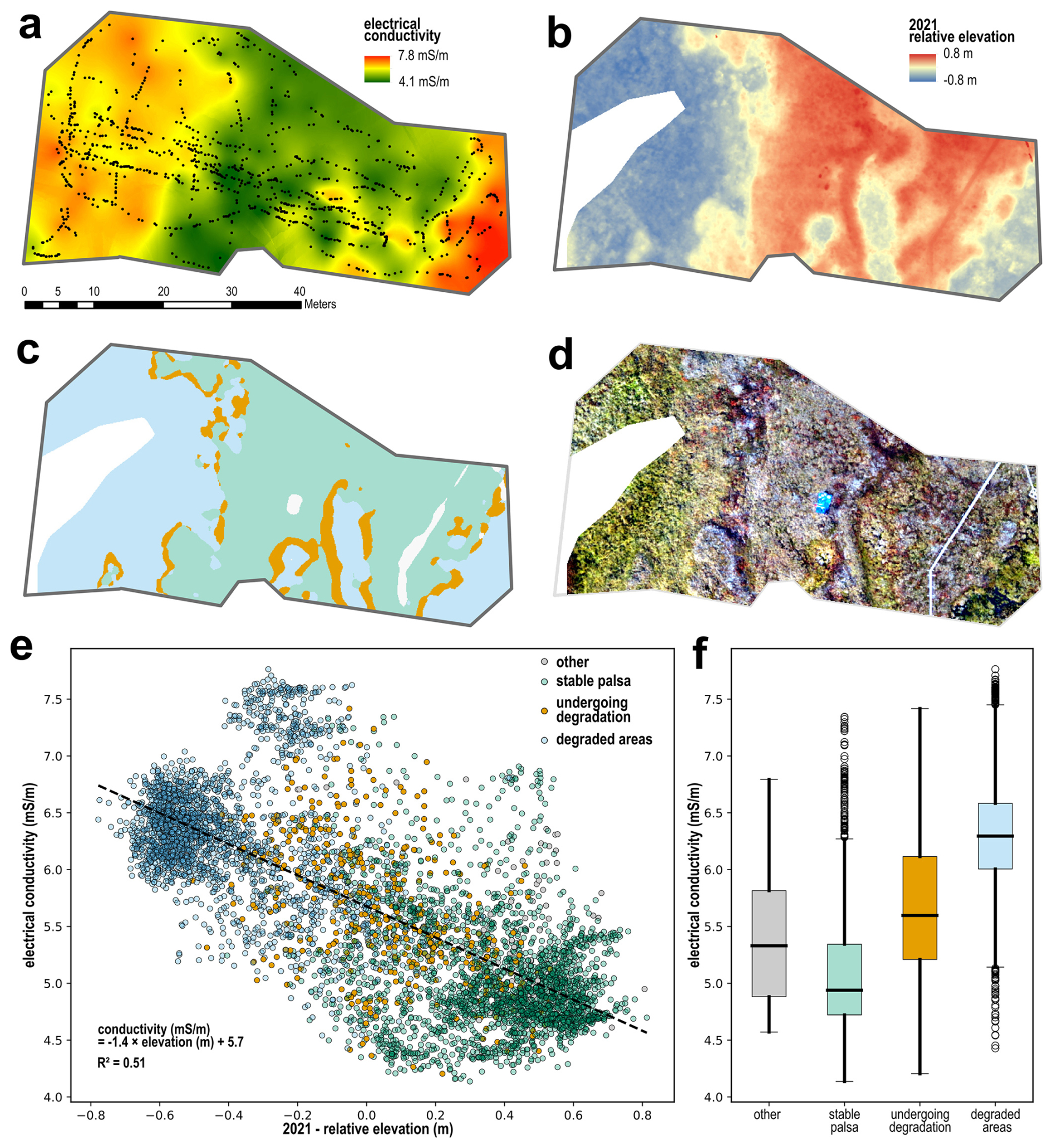
Figure 7 Evolution of electrical conductivity data and comparison with the results of the biennial classification model (between 2019 and 2021). (a) Continuous map of electrical conductivity obtained by simple kriging of point data; (b) Relative elevation data corrected by removal of the bowl-shape effect; (c) Classification model results for 2021 (see Fig. 4b for the entire model); (d) RGB imagery data for 2021; (e) Linear regression between electrical conductivity and relative elevation for the different classes; (f) Boxplots of the electrical conductivity per land cover class. Data processing extent as in Fig. 2a. Color code as in Fig. 4.

3.3 Palsa degradation leads to increases in areas with high soil moisture and open water

Lowland thermokarst development is typically associated with drastic modifications in landscape hydrology, redox conditions, vegetation species composition, organic carbon stability and GHG emissions (e.g., Palace et al., 2018; Patzner et al., 2020; Varner et al., 2022). Such is the case in Stordalen, where, using classification models from the 2014–2022 time series (Fig. 6), we observe a decrease in the stable palsa areal extent of ∼ 8 % a⁻¹ between 2014 and 2022 (Fig. 6a). We further note that the fraction of the open water class has more than doubled in size between 2014 and 2022. This is consistent with the general trend towards wetter conditions documented at Stordalen (e.g., Varner et al., 2022), but inter- and intra-annual variability in hydrological conditions may also contribute to differences between surveys (e.g., 2018 appears to have been drier), as fluctuations in water-table depth and precipitation are expected in the mire (e.g., Bäckstrand et al., 2008; ICOS Sweden, 2023; Petrescu et al., 2008). These rates of surface area change appear to be higher, but remain within the same order of magnitude as the biennial model (2019–2021). It should be noted that the spatial extent is not identical to that presented in Sect. 3.2 (see Fig. 2a). Furthermore, the model from the 2014–2022 UAS time series does not use terrain morphology data (relative elevation and slope) for classification. As a result, the overall accuracies and F-scores (Fig. 6a) are weaker than for the biennial model (Table 2), for which topography data were used. We believe, however, that it can provide an indication of trends, and has the advantage of enabling tracking of the “open water” class surface area, which is not possible with the biennial model.

Electrical conductivity (EC) data obtained from electromagnetic induction (EMI) range from 4.1 to 7.8 mS m⁻¹ over the survey area (Fig. 7a) and are well aligned with relative elevation and the predicted degradation classes (Fig. 7b–e). This range of values allows for the use of the Low Induction Number (LIN) hypothesis, enabling the estimation of soil EC from the quad-phase component of the measured field, as the LIN assumption is met (McNeill, 1980). The EC values are relatively low, reflecting the absence or minimal presence of clay and low salinity. This observation aligns with the hydrological regime of the area, where surface water is primarily rain-fed, with limited inputs from mineralized groundwater or subsurface flow (e.g., Henrion et al., 2024). The central part of the area exhibits the lowest EC values, which correspond to the highest elevation and stable palsa area. This pattern is consistent with the hydrological gradient, as higher elevations typically exhibit better drainage, reducing water content and, consequently, EC. Electrical conductivity patterns also align with the distribution of vegetation types, as shown in the RGB orthophoto, with stable palsa associated with low-growing ericaceous and woody plants and degraded areas covered by green sedges (Fig. 7d). Notably, areas with more developed vegetation correspond to areas with higher EC values, likely due to increased water and nutrient availability in these zones, which supports greater plant growth. A relationship is observed between EC and relative elevation (R² = 51 %; Fig. 7e), further emphasizing the influence of micro-topography on soil hydrology and conductivity. Significant differences in EC are also observed between the different degradation classes (p-value from Kruskal-Wallis test < 10⁻³ and p-values from Wilcoxon rank-sum tests < 10⁻³; Fig. 7f). Degraded areas consistently exhibit higher EC values compared to stable palsa, further supporting the role of water content as a key factor driving changes in EC. Since high EC is indicative of increased water content (assuming other factors such as clay content, salinity, and soil mineralogy remain constant), this suggests that palsa degradation induces a net increase in soil moisture. This process is likely to shift the soil environment toward more anaerobic conditions, reducing organic matter geochemical stability (e.g., Monhonval et al., 2023; Patzner et al., 2020), but also favoring processes such as methanogenesis (e.g., Varner et al., 2022), which could have significant implications for greenhouse gas emissions.

3.4 Implications of palsa degradation for both organic carbon stability and greenhouse gas emissions

The land cover is generally a very important predictor for both the distribution of organic carbon and GHG emissions (e.g., Siewert, 2018; Varner et al., 2022). For first order estimates of the evolution of OC stocks or GHG emissions in Stordalen, we used a space-for-time approach using the thematic maps developed in this study (Sect. 3.2). To this end, Patzner et al. (2020) showed a drop in the concentration of TOC and MAOC along the degradation gradient in the Stordalen mire. Using estimates of the surface area degraded between 2019 and 2021, we calculated that – for the 14 ha of this study site and for a palsa depth of 23 cm – palsa degradation results in 12 × 10³ kg a⁻¹ of TOC becoming vulnerable to decomposition, including 3 × 10³ kg a⁻¹ of MAOC (calculation details are available in Tables B1 and B2). This corresponds to a balance of −1.6 % a⁻¹ relative to the TOC stock in 2019 and −3.3 % a⁻¹ relative to the MAOC stock in 2019. These are estimates of TOC or MAOC stocks that are made vulnerable annually as a result of palsa degradation and represent first order estimates. The actual proportion and timing of OC export or GHG emissions remain unknown. With regard to GHG emissions, Sjögersten et al. (2023) showed a substantial increase in methane emissions from stable palsa plant communities to degrading and inundated plant communities, highlighting the importance of not only the degree of degradation, but also the vegetation community composition dictating differences in the magnitude of CH₄ emissions. Varner et al. (2022) showed that the net radiative forcing of the Stordalen mire shifted from a slightly negative value before 2000 to a strongly positive value after that date, and increased again in 2014. As a result of accelerated degradation (Sect. 3.2), we can expect the radiative forcing to become even more positive through increased CH₄ emissions, as the mire becomes wetter (Sect. 3.3). Likewise, Łakomiec et al. (2021) measured field-scale CH₄ emissions at Stordalen of 2.7 ± 0.5 and 8.2 ± 1.5 $\mathrm{g}-\mathrm{C}{\mathrm{m}}^{-\mathrm{2}}{\mathrm{a}}^{-\mathrm{1}}$ (mean annual emissions) for the palsa and thawing surfaces, respectively. With the palsa degradation rates calculated in this study, this would mean that the average annual emissions would increase from ∼ 6.3 $\mathrm{g}-\mathrm{C}{\mathrm{m}}^{-\mathrm{2}}{\mathrm{a}}^{-\mathrm{1}}$ in 2019 to ∼ 6.4 $\mathrm{g}-\mathrm{C}{\mathrm{m}}^{-\mathrm{2}}{\mathrm{a}}^{-\mathrm{1}}$ in 2021 for the entire mire, i.e., an increase of ∼ 1.1 % a⁻¹.

3.5 From local to Arctic scale

Predicting the response of permafrost terrains to climate change and disturbances beyond local scales is extremely difficult (Nicolsky et al., 2017). Discrepancies very often exist between circumpolar-scale and local-scale models. This is, for instance, the case for total organic carbon maps, where local estimates (e.g., Fuchs et al., 2015; Palmtag et al., 2015; Siewert, 2018) deviate from circumpolar estimates (Hugelius et al., 2013, 2014). The large-scale estimates used in global or regional models fail to reflect the heterogeneity observed in this typical Arctic environment, where soil properties are highly variable on scales of a few tens of centimeters and often defined by landforms and their degradation trajectory (Siewert et al., 2021), as is the case in Abisko and in many other Arctic environments. Yet, the importance of wetlands for organic carbon stocks at the Arctic scale has long been pointed out (e.g., Siewert, 2018). When the temporal evolution component is added, these global estimates are even more difficult to achieve. In the present study, we saw that the parameters of relative elevation and slope (and their change) were key components in detecting the formation of thermokarst in lowland peat-rich landscapes. However, digital elevation models across the Arctic are generated from multi-annual data, e.g. 15 years for ArcticDEM (Porter et al., 2023). Although efforts are being made to generate annual elevation models, e.g., for the Greenland Ice Sheet (Winstrup et al., 2024), such circumpolar-scale data are not yet available. Still, similar studies could be conducted on multiple thermokarst landscapes across the Arctic and at different latitudes. This approach would provide valuable insight into the variability of degradation rates, which could then be included in models such as those used in Turetsky et al. (2020) or Hugelius et al. (2020). A promising approach is the use of InSAR to detect thermokarst and quantify permafrost degradation as well as resulting GHG emissions (van Huissteden et al., 2021; Sjögersten et al., 2023; Valman et al., 2024), but de la Barreda-Bautista et al. (2022) highlight the relevance of using UAS data to ground-truth such efforts. A further avenue for monitoring the development of thermokarst landscapes on a circumpolar scale would be to measure the evolution of soil moisture over time. In that respect, drone-borne ground-penetrating radar (GPR) has demonstrated significant potential for high-resolution mapping of soil electrical conductivity and soil moisture (Wu et al., 2019; Wu and Lambot, 2022). Unlike other proximal or remote sensing sensors, which are limited to surface property characterization, GPR provides depth-resolved information, enabling the detection of subsurface changes linked to permafrost degradation, such as increases in soil moisture and ground subsidence.

4 Conclusions

We examined a gradient of lowland thermokarst development at Stordalen mire, Abisko, Sweden, extending from well-drained stable palsas to inundated fens affected by ground subsidence. Palsa degradation was quantified using RGB imagery and topographic data from UAS surveys between 2019 and 2021, together with a coarser assessment based solely on RGB imagery spanning 2014–2022. Our results lead to the following conclusions:

• 1.

  Topography is a critical parameter for determining the evolution of palsa degradation. Including relative elevation and slope data increases the overall classification accuracy from 41 % to 77 %, highlighting the value of topographic information for identifying palsa degradation. Slope further enables better detection of the early stages of degradation.

• 2.

  We observe a clear acceleration of degradation in Stordalen between 2019 and 2021, with a decrease in stable palsa area of 3.3–3.6 % a⁻¹ compared to previous studies for 1970–2000 (∼ 0.3 % a⁻¹; Christensen et al., 2004) and 2000–2014 (∼ 0.1 % a⁻¹; Varner et al., 2022).

• 3.

  Our coarser evaluation based solely on RGB imagery leads to higher rates for the period 2014–2022 and likewise demonstrates a twofold increase in the surfaces of open water. Electromagnetic induction data also supports the increase in soil moisture as palsas degrade, which is likely to alter the soil environment towards more anaerobic conditions.

• 4.

  By combining the rates of palsa degradation from this study with existing data on carbon concentration, stability and release from the study site, we estimated that palsa degradation at Stordalen may expose approximately 12 × 10³ kg of organic carbon annually within the top 23 cm of soil, of which roughly 25 % is mineral-interacting organic carbon. Likewise, average annual emissions would increase from ∼ 6.3 $\mathrm{g}-\mathrm{C}{\mathrm{m}}^{-\mathrm{2}}{\mathrm{a}}^{-\mathrm{1}}$ in 2019 to ∼ 6.4 $\mathrm{g}-\mathrm{C}{\mathrm{m}}^{-\mathrm{2}}{\mathrm{a}}^{-\mathrm{1}}$ in 2021 for the entire mire, i.e., an increase of ∼ 1.1 % a⁻¹.

Scaling this approach to the circumpolar Arctic poses a major challenge. Small topographic changes associated with thermokarst development are not captured by satellite images, making the detection of this process challenging. Applying the methodology developed in this study to cover a large number of study sites would make it possible to assess the spatial variability of degradation rates and thus serve as an input for net ecosystem carbon balance models.

Appendix A: Additional methodological information

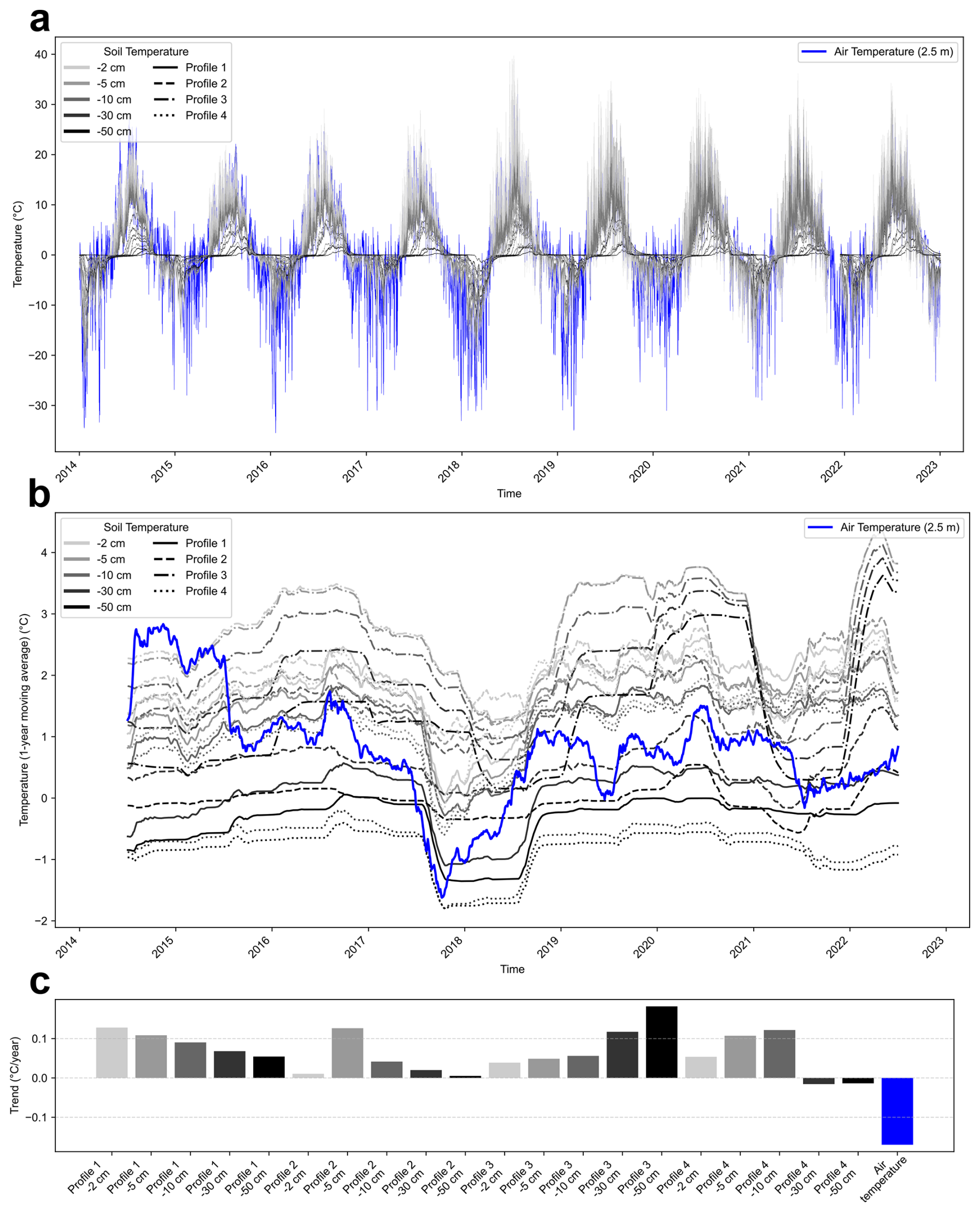
Figure A1 Air and ground temperatures at Stordalen between 2014 and 2022. (a) half-hourly air temperature at 2.5 m and soil temperatures from 4 profiles at 2, 5, 10, 30, and 50 cm depth (ICOS Sweden, 2023); (b) annual moving averages calculated on these same data; (c) significant trends in temperature changes calculated from moving averages (p-values < 10⁻³).

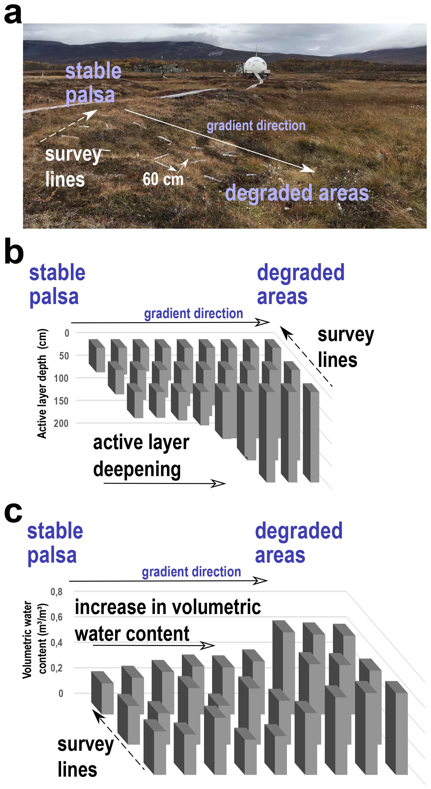
Figure A2 Conceptual model and illustration of the permafrost degradation gradient at the Stordalen Mire. (a) measuring grid along the gradient (photo: Sophie Opfergelt; 30 September 2021) where point-to-point distance is indicated for scale; (b) evolution of active layer depth along the gradient; (c) evolution of the volumetric water content along the gradient.

Table A1 Summary of the different unoccupied aircraft system (UAS) data used in this study. $\mathrm{a}.\mathrm{g}.\mathrm{l}.$ = above ground level.

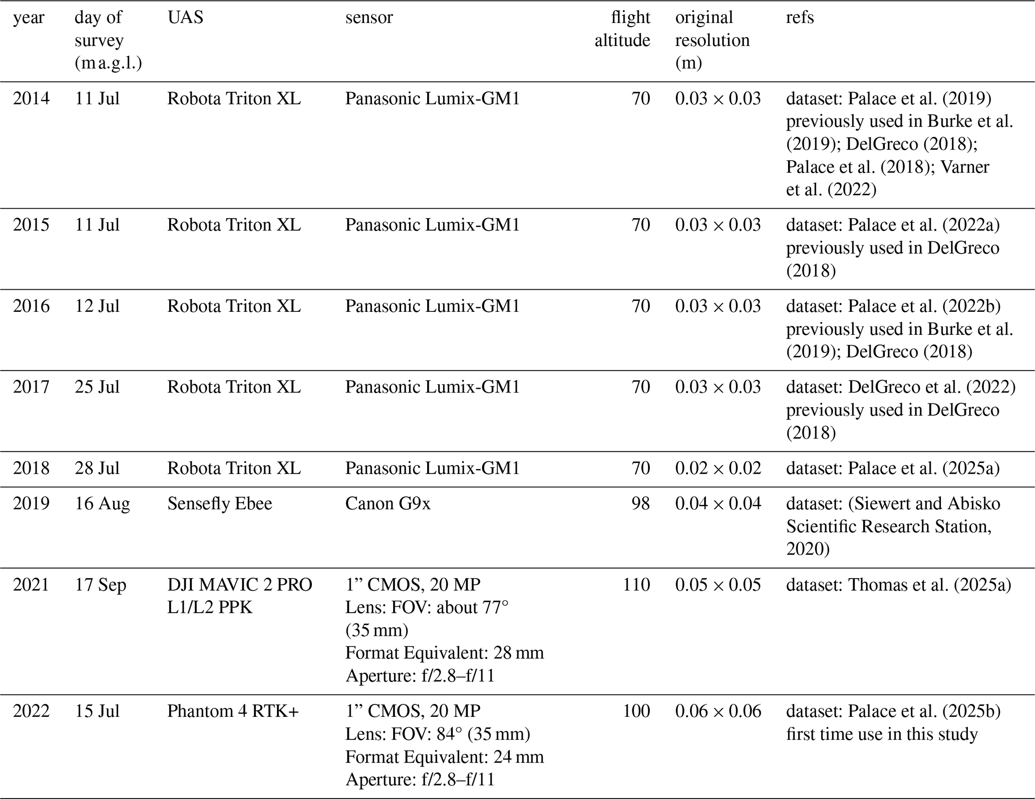
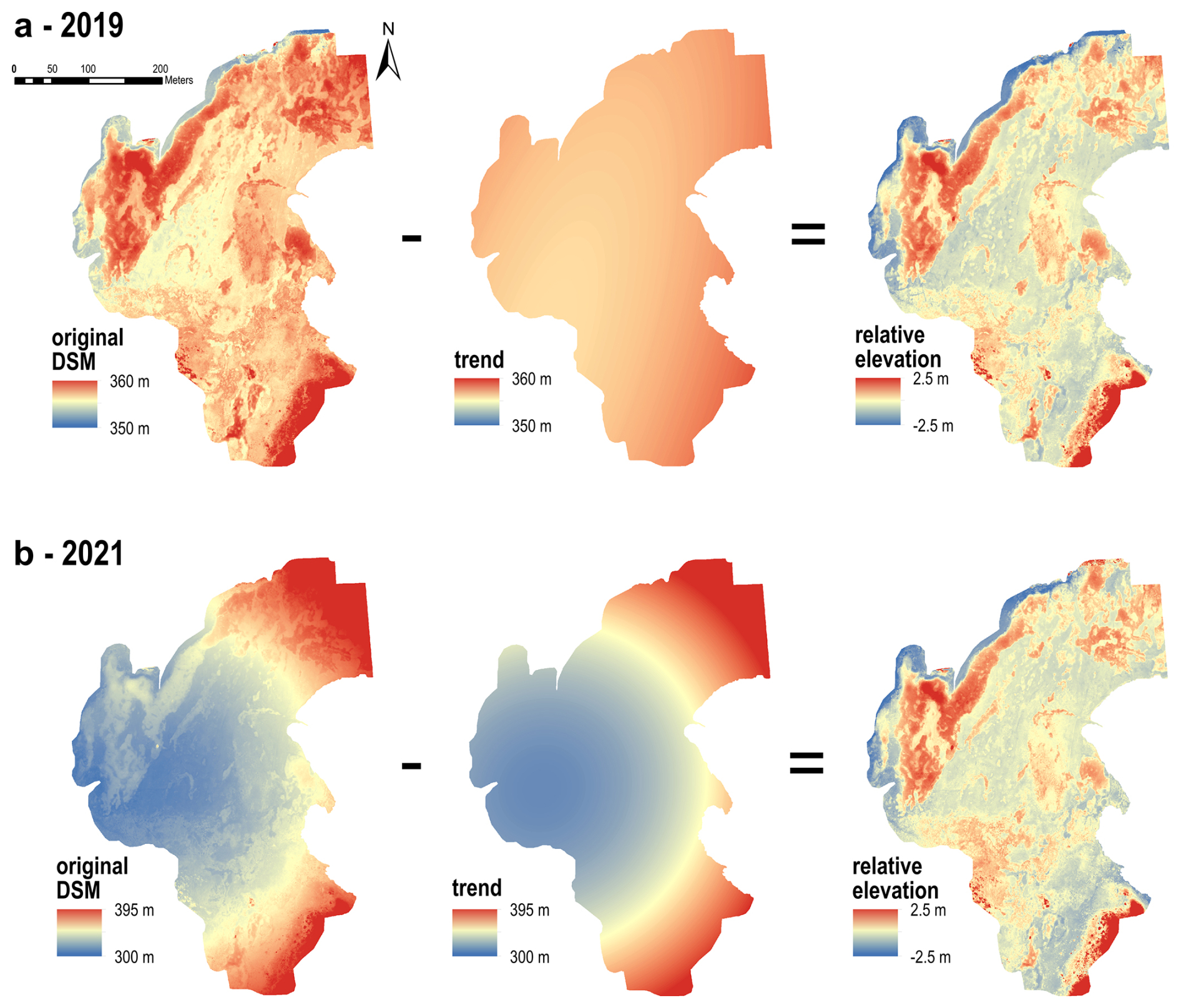
Figure A3 Removing of the bowl-shape effect from elevation data (DSM) for (a) 2019 and (b) 2021. The processing involves (i) extraction of the original elevation band on a regular 5 m × 5 m grid; (ii) on this grid, exclusion of the data that diverge by more than 3 times the standard deviation, and calculation of the second-order trend from those data that from the original elevation data; (iii) calculation of residuals by subtraction of the 2nd-order trend from the original data. The result represents the relative elevation data (corrected DSM).

Table A2 Distribution of training points for each class.

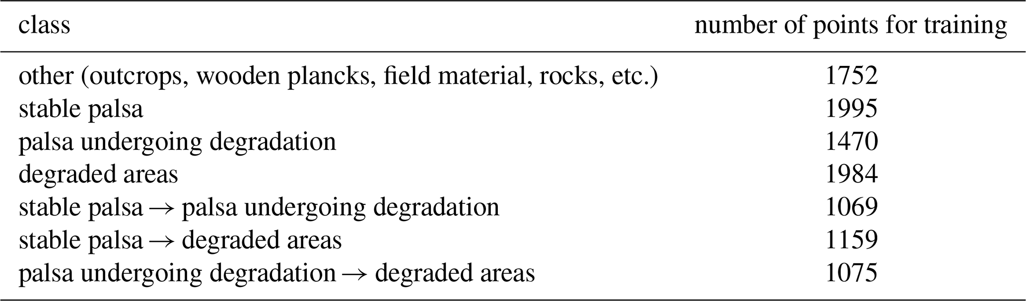
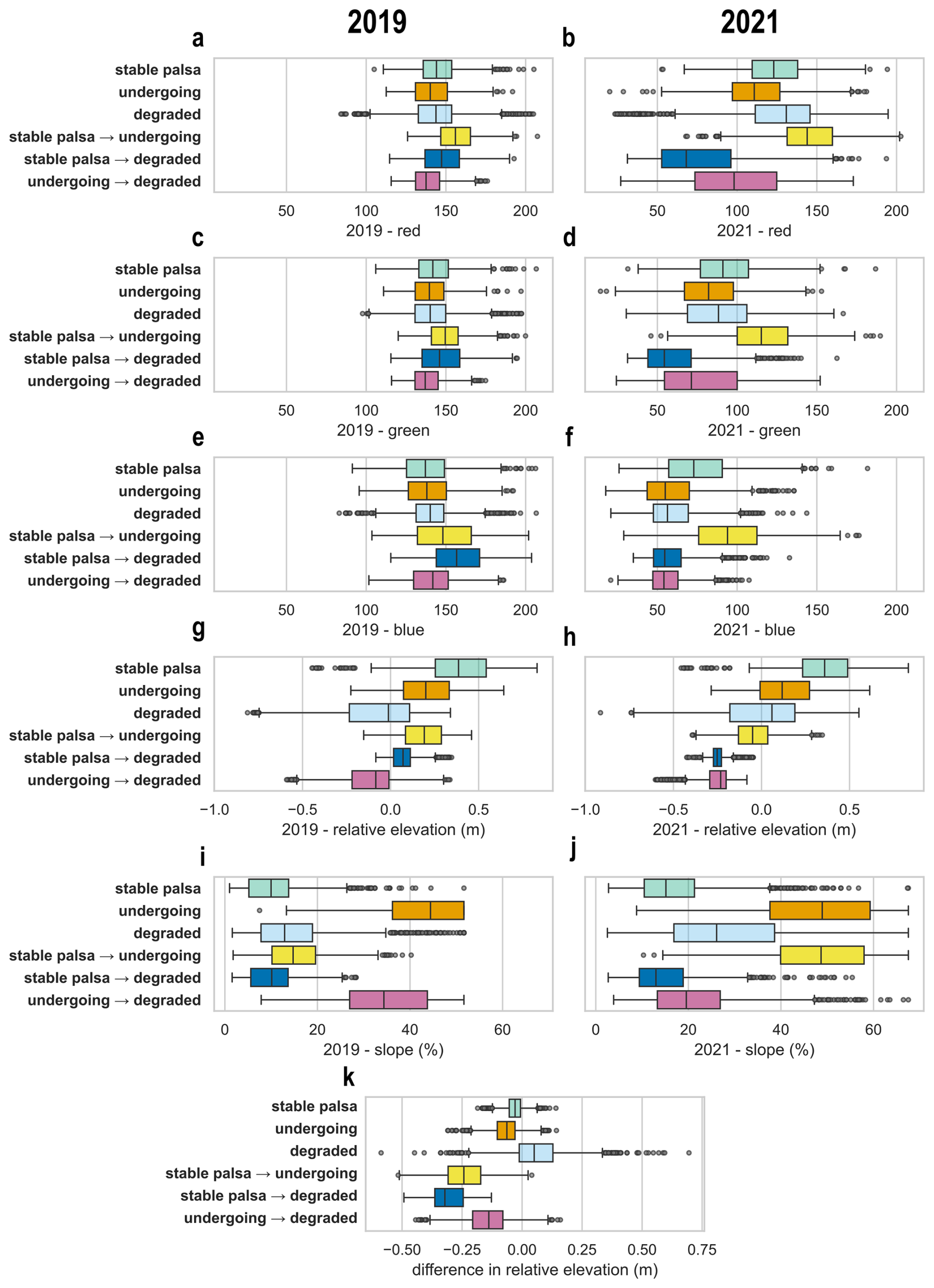
Figure A4 Distribution of the selected input data values across the training areas of the classification model, namely (a, b) red color, (c, d) green color, (e, f) blue color, (g, h) relative elevation data corrected by removal of the bowl-shape effect, (i, j) slope values derived from the original DSM and (k) the difference in relative between 2019 and 2021. DSM = digital surface model. Color code as in Fig. 4.

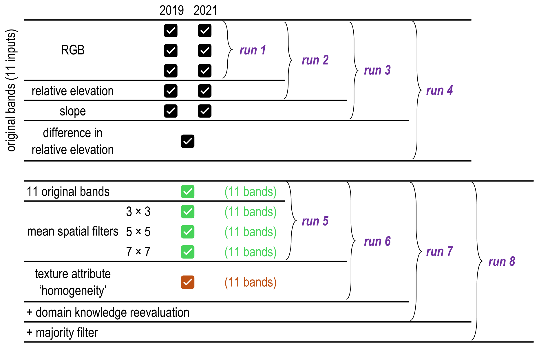
Figure A5 Workflow of the different runs of the model with successive additional data inputs and post-processing steps.

Appendix B: Tables for scaling up organic carbon stocks

Table B1 Method for scaling up organic carbon stocks from the use of the classified landscape. TOC = total organic carbon; MAOC = mineral-associated organic carbon. Thickness, bulk density, TOC and MAOC data from Patzner et al. (2020). OH = organic horizon; TZ = transition zone; MH = mineral horizon.

$$\begin{array}{}\text{(B1)}& \begin{array}{rl}& \text{mineral\hspace{0.17em}\hspace{0.17em}matter\hspace{0.17em}\hspace{0.17em}stock}{\left({\displaystyle \frac{{\mathrm{kg}}_{\mathrm{mineral}\mathrm{matter}}}{{\mathrm{m}}^{\mathrm{2}}}}\right)}_i\\ =& \left({\text{bulk\hspace{0.17em}\hspace{0.17em}density}}_i\left({\displaystyle \frac{{\mathrm{kg}}_{\mathrm{soil}}}{{\mathrm{m}}^{\mathrm{3}}}}\right)\times {\text{thickness}}_i\left(\mathrm{m}\right)\right)\\ & -\left(\left({\text{bulk\hspace{0.17em}\hspace{0.17em}density}}_i\left({\displaystyle \frac{{\mathrm{kg}}_{\mathrm{soil}}}{{\mathrm{m}}^{\mathrm{3}}}}\right)\times {\text{thickness}}_i\left(\mathrm{m}\right)\right.\right.\\ & \left.\times {\text{ OC\hspace{0.17em}\hspace{0.17em}content}}_i\left({\displaystyle \frac{{\mathrm{kg}}_{\mathrm{OC}}}{{\mathrm{kg}}_{\mathrm{soil}}}}\right)\right)\\ & \left.\times \mathrm{1.724}\left({\displaystyle \frac{{\mathrm{kg}}_{\mathrm{organic}\mathrm{matter}}}{{\mathrm{kg}}_{\mathrm{OC}}}}\right)\right)\end{array}\end{array}$$

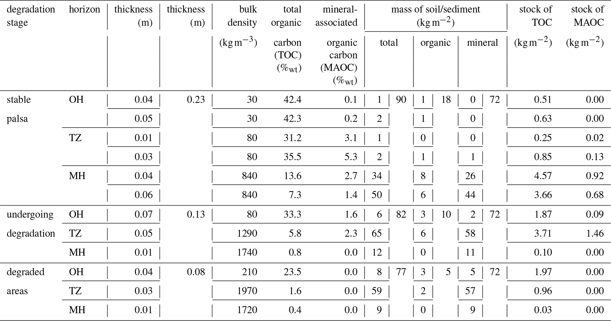
Table B2 Results of scaling up organic carbon stocks from the use of the classified landscape. TOC = total organic carbon; MAOC = mineral-associated organic carbon. Surfaces in 2019 and 2021 from Fig. 4.

Appendix C: Additional results

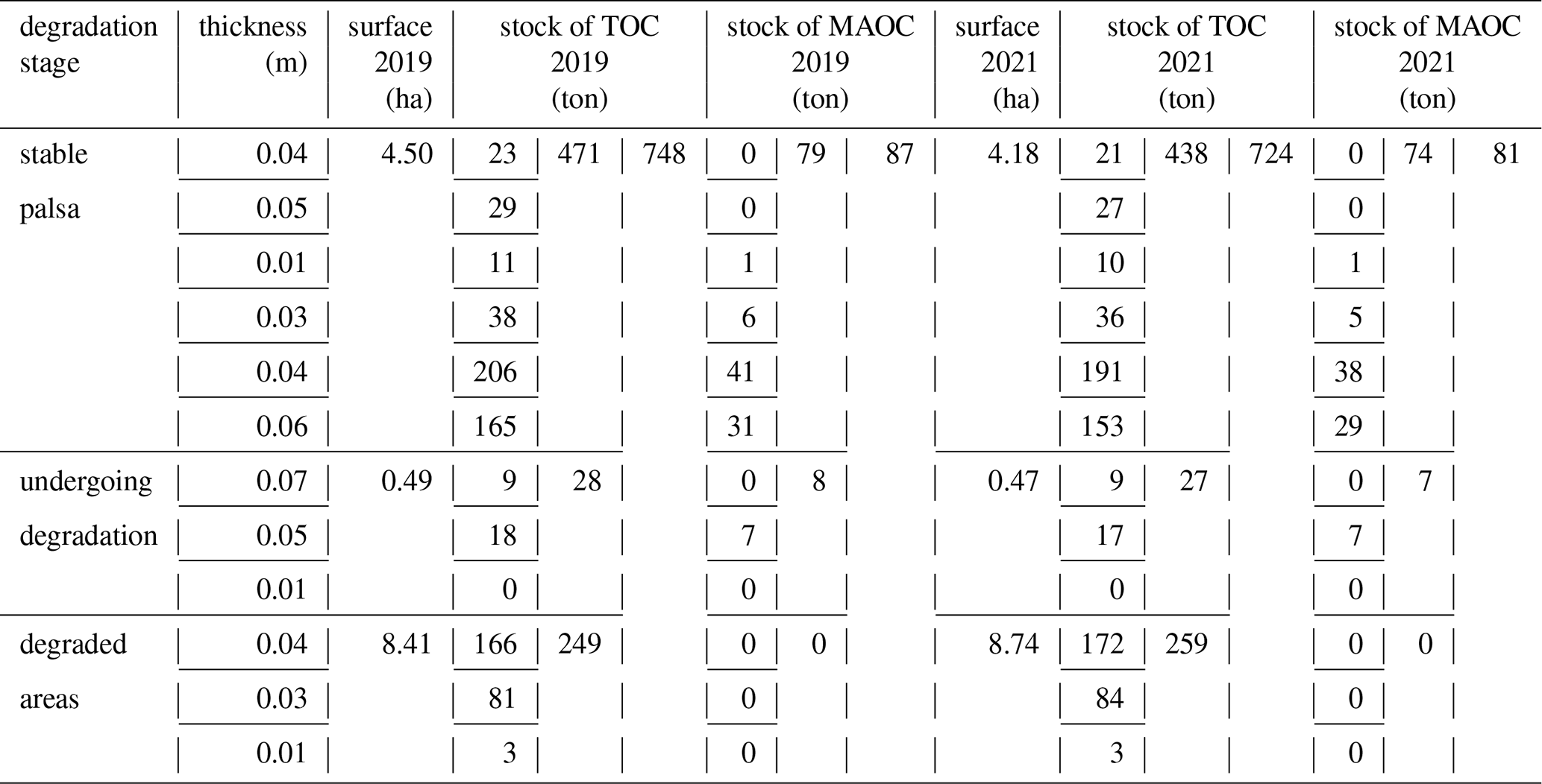
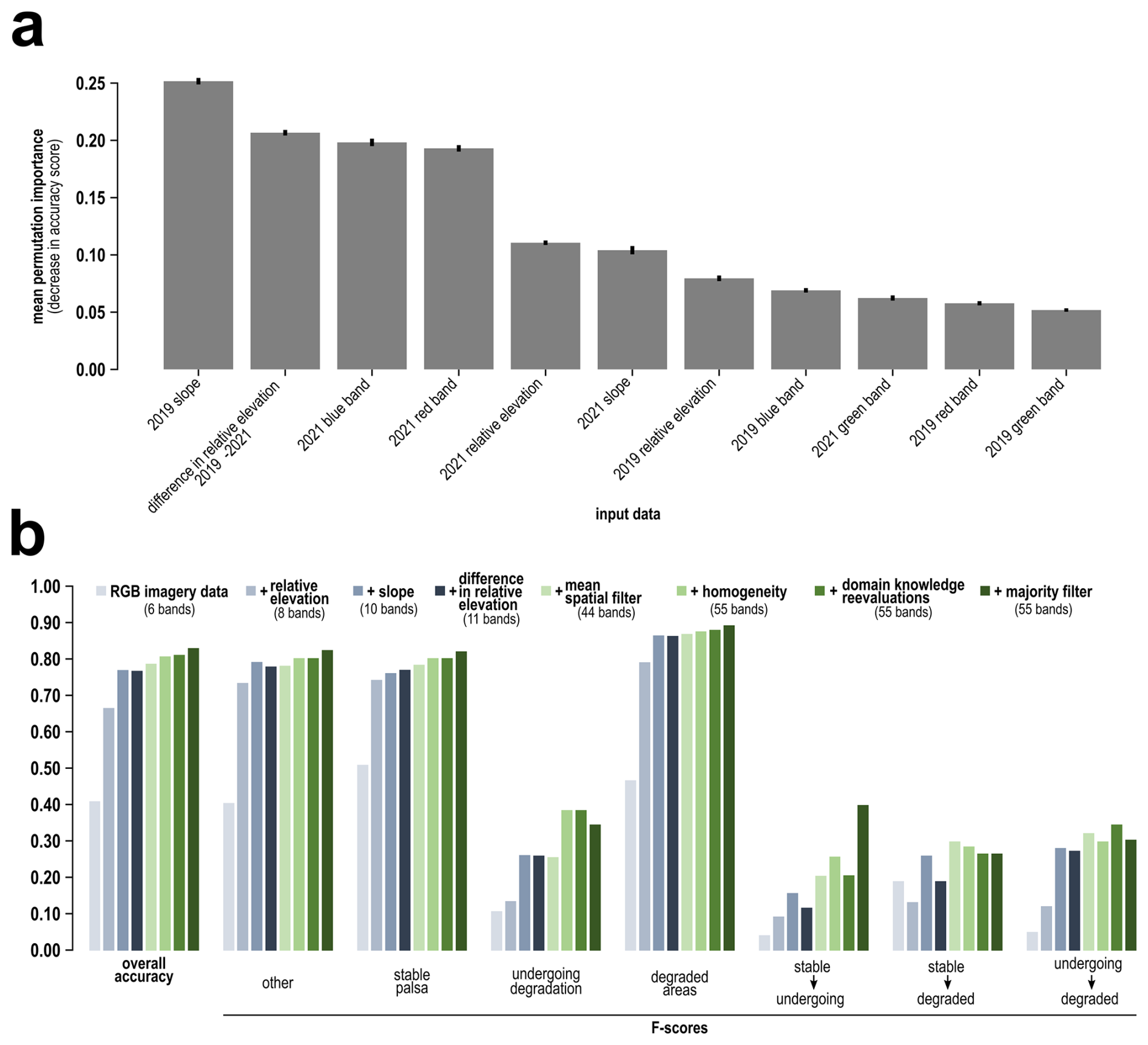
Figure C1 Performance evaluation of the biennial (2019–2021) model. (a) Mean permutation importance (scikit-learn built-in function) of each input data in the model, measured as the decrease in accuracy when the input data values are randomly shuffled. The error bars indicate the standard deviation of importance across 10 permutations. (b) Evolution of the overall accuracy and F-scores of the classes based on the input data for the classification. Mean spatial filter = mean of pixel values in 3 × 3, 5 × 5 and 7 × 7 moving windows. Homogeneity = texture attribute “homogeneity” based on the gray-level co-occurrence matrix applied within a 21 × 21 moving window. Domain knowledge reevaluation = refinement using elevation differences and model scores to ensure alignment with domain knowledge (see Sect. 2.4). majority filter = filter using windows of increasing size up to 11 pixel × 11 pixel, to reduce noise and enhance classification consistency.

Table C1 Confusion matrix for the classification model and precision, recall and F-score for each cover class after classes aggregation for 2019. This model uses 55 bands as input data, namely (i) 11 bands with original data (3 spectral bands, relative elevation and slope for the years 2019 and 2021 as well as the difference in relative elevation between 2019 and 2021) along with (ii) 3 × 11 bands with spatial filters (mean and standard deviation) over windows of increasing size, i.e. 3 × 3, 5 × 5 and 7 × 7, and finally (iii) the 11 bands from the texture attribute “homogeneity”. The classification output was then filtered with a moving window of 11 pixel × 11 pixel. Bold values represent the diagonal of correct predictions.

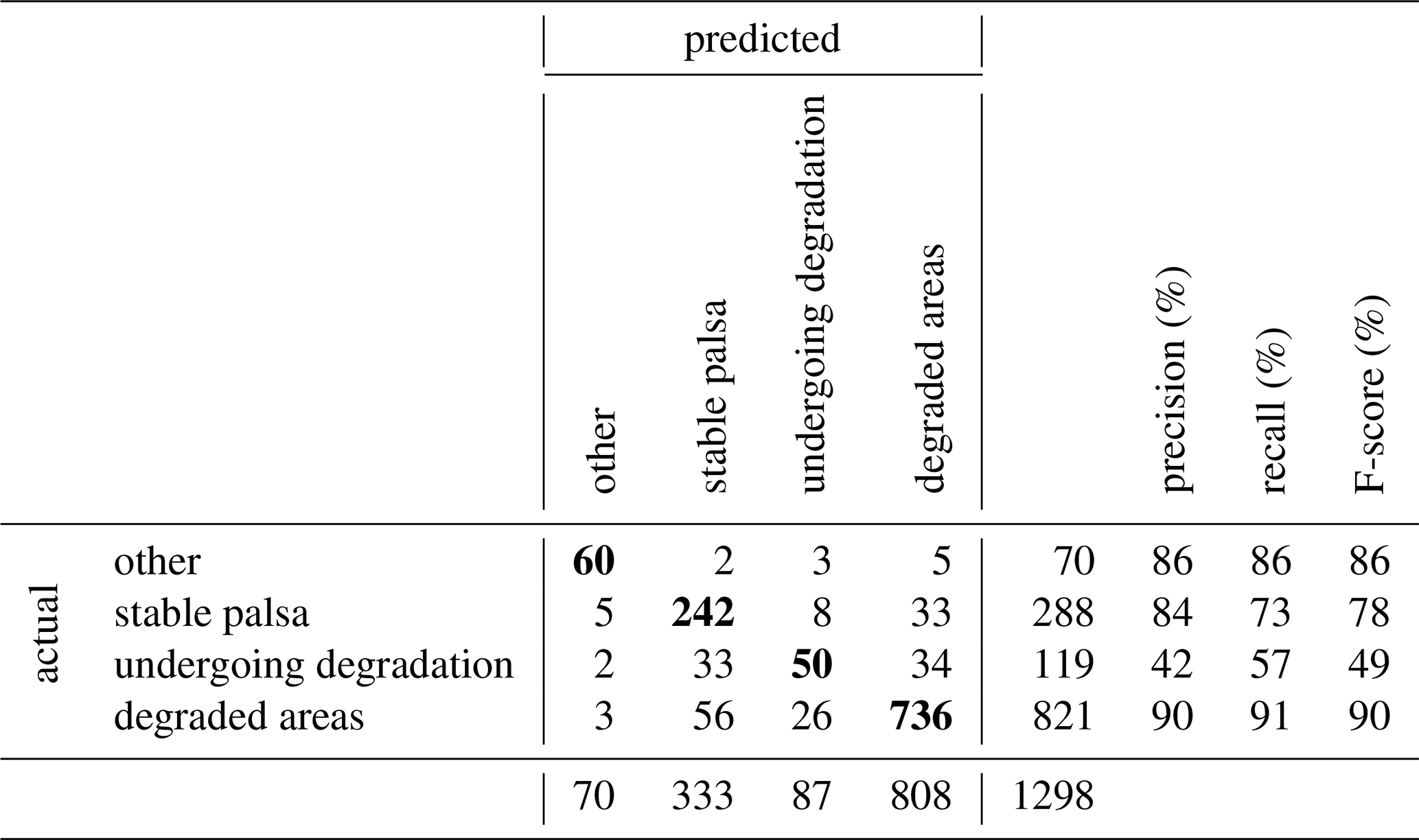
Table C2 Confusion matrix for the classification model and precision, recall and F-score for each cover class after classes aggregation for 2021. This model uses 55 bands as input data, namely (i) 11 bands with original data (3 spectral bands, relative elevation and slope for the years 2019 and 2021 as well as the difference in relative elevation between 2019 and 2021) along with (ii) 3 × 11 bands with spatial filters (mean and standard deviation) over windows of increasing size, i.e. 3 × 3, 5 × 5 and 7 × 7, and finally (iii) the 11 bands from the texture attribute “homogeneity”. The classification output was then filtered with a moving window of 11 pixel × 11 pixel. Bold values represent the diagonal of correct predictions.