Temporal evolution of the Petermann Ice Shelf estuary constrained by satellite remote sensing observations

Supraglacial rivers may reduce ice-shelf instability by draining meltwater from the ice-shelf surface, limiting loading-induced stresses from ponded meltwater. However, if a supraglacial river incises to below sea level at the ice-shelf front, forming an estuary, this effect may be negated. Water flow reversal in the estuary loads the ice shelf, which induces flexural stress, limits meltwater export, and enhances melting. This phenomenon was first identified at Petermann Ice Shelf, Northern Greenland. A key factor in determining when and where ice-shelf estuaries form is river incision rate – the decrease in channel bed elevation over time. Here we present a novel method for calculating incision rate in supraglacial rivers from paired multispectral WorldView imagery and corresponding ArcticDEM strips, applied over Petermann Ice Shelf during the 2014 and 2016 melt seasons. Incision rates differ substantially between the two years, peaking near the river/estuary mouth in 2014, and reaching a minimum there in 2016. Based on visual interpretation of WorldView imagery and modelled runoff from 2013–2018, we conclude these contrasting incision patterns are caused by the formation of the estuary and resultant flow reversal which shifts the dominant melt pattern from vertical incision to lateral erosion. Further, our analysis reveals a cyclical pattern of estuary formation starting in 2014, with the estuary disappearing and reforming annually; this pattern is interrupted in 2018, when a transverse rift bisects the channel. This indicates that estuary presence, even when spatially and temporally limited, may contribute to ice-shelf instability.

1 Introduction

Ice shelves can play a key role in mitigating the contributions of ice sheets to global sea level rise by buttressing outlet glaciers, thereby slowing upstream glacier flow (e.g., Gudmundsson et al., 2019). In Greenland, ice-shelf retreat has been ongoing since at least 1990, with three ice shelves collapsing completely over this period (Millan et al., 2023; Moon and Joughin, 2008). Today, there are only five major ice shelves remaining in Greenland: Petermann, Steensby, Bistrup Brae/Storstrømen, Ryder, and Nioghalvfjerdsbrae (79N; Millan et al., 2023; Wang et al., 2024). Of these, four have experienced grounding zone retreat since 1992, and total ice shelf area in Greenland has decreased from 4413 km² in 2000 to 3513 km² in 2022 (Millan et al., 2023). In Antarctica, more than 75 % of the coastline is buttressed by ice shelves (Fürst et al., 2016), and ice-shelf retreat, mostly confined to West Antarctica, has been balanced by gradual advance in East Antarctica (Andreasen et al., 2023). Surface melt on ice shelves is driven by atmospheric forcing, which is projected to increase in intensity over both ice sheets throughout the 21st century (Smith et al., 2020). Ice-shelf dynamics and stability are impacted by how surface meltwater is stored, transported, and exported (Bell et al., 2018). Many ice shelves in both Greenland and Antarctica form extensive surface hydrologic networks each summer, some of which include large supraglacial rivers that flow into the ocean (e.g., Petermann in Greenland, Nansen in Antarctica). Often, rivers on ice shelves form in the surface depressions over basal channels, and the presence of these basal channels has been shown to have a destabilizing effect on ice shelves by driving fracture formation perpendicular to ice flow (Dow et al., 2018). In some cases, these surface rivers can export large volumes of meltwater from the ice shelf into the ocean, limiting loading-induced stresses from ponded meltwater (Banwell et al., 2013) and thus mitigating ice-shelf breakup (Banwell, 2017; Bell et al., 2017). However, if a supraglacial river incises the ice surface below sea level, forming an ice-shelf estuary (Fig. 1), this mitigating effect may be negated, and further, additional instability may be introduced by the resultant tidal loading (Boghosian et al., 2021).

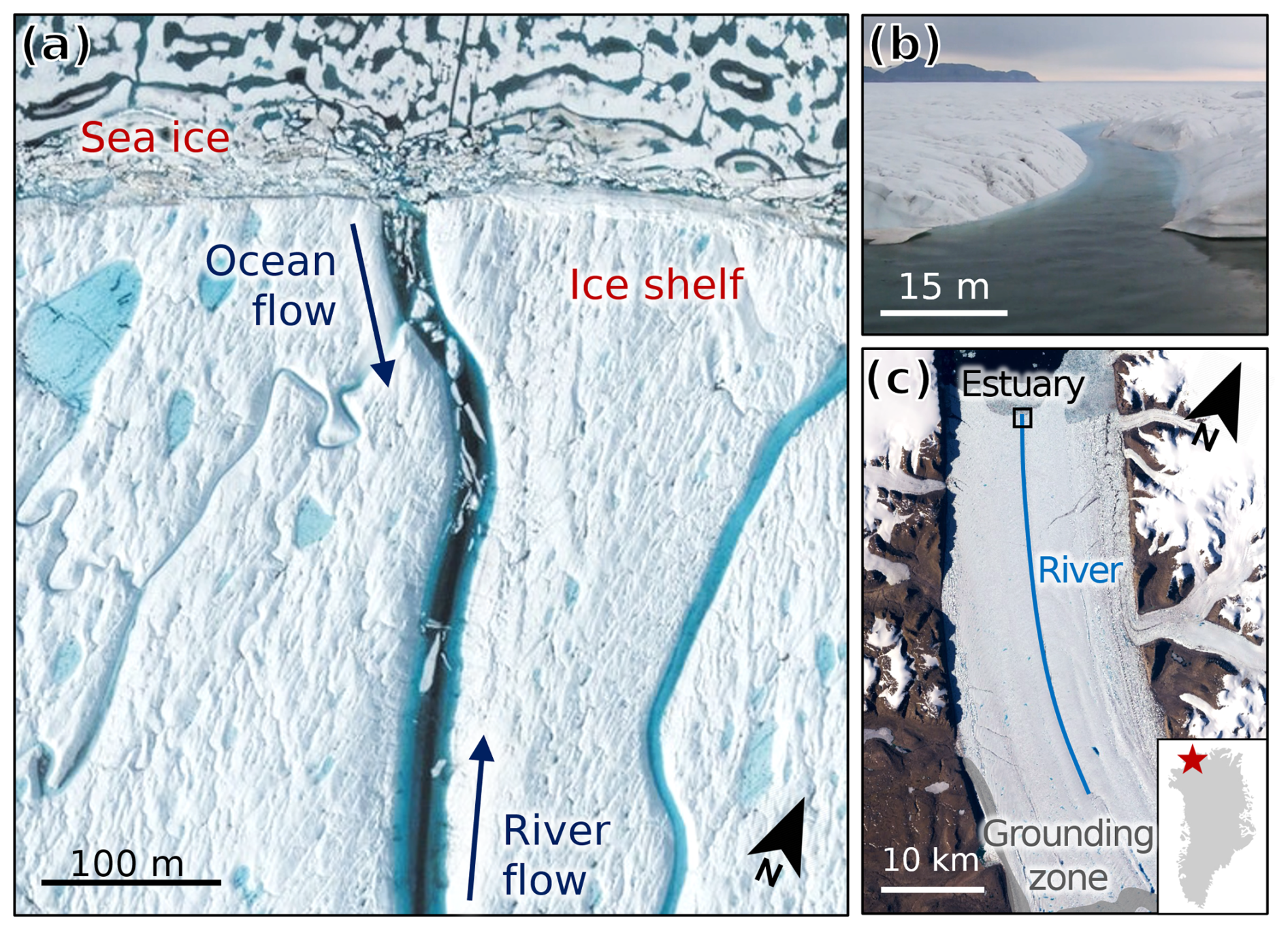
Figure 1 Petermann Ice Shelf estuary: (a) WorldView-2 image from 24 July 2018 of the ice-shelf estuary (black box in panel c) with sea ice flowing upstream towards the grounding zone during ocean-induced flow reversal (© Vantor 2018), (b) view of the ice-shelf estuary from the ocean in summer 2015 (credit 77th Parallel), and (c) Sentinel-2 image from 25 July 2018 showing the locations of the ice-shelf estuary (square black box), the central ice-shelf river (blue line), and the grounding zone (grey shading; Ciracì et al., 2023).

An ice-shelf estuary was first discovered at Petermann Ice Shelf in Northern Greenland, where it was initially identified from WorldView-2 imagery showing sea ice floating upstream towards the grounding zone in its large supraglacial river (Fig. 1a; Boghosian et al., 2021). Terrestrial estuaries form where rivers and oceans meet; on an ice shelf, estuaries form when the bed of a supraglacial river incises below sea level allowing seawater intrusion. At the mouth of the estuary cold, fresh meltwater mixes with warmer, saline seawater (Boghosian et al., 2021). Driven by tides, river flow can also reverse, drawing warm seawater inward onto the ice shelf (Boghosian et al., 2021; Geyer and MacCready, 2014). This water flow reversal may act to load the ice shelf, which changes its stress field. This is due to both the inflow of seawater into the channel, as well as the decreased meltwater export from the ice shelf into the ocean. Mixing of freshwater and seawater in the channel, the extent to which remains unknown, is likely driven by wind and tidal fluctuations. Together, the enhanced loading and limited meltwater export may contribute to destabilizing the ice shelf.

In addition to the Petermann Ice Shelf estuary, Boghosian et al. (2021) hypothesize that a second estuary has formed on Ryder Ice Shelf in Greenland, but to date, no additional estuaries have been identified. As atmospheric temperatures rise and melt seasons continue to lengthen on the Greenland and Antarctic ice sheets, driving increased surface melt (Hanna et al., 2024; Jourdain et al., 2025), ice-shelf estuaries are expected to persist in Greenland for as long as ice shelves remain and begin forming around Antarctica within 30 years (Boghosian et al., 2021). To improve projections of when and where estuaries are likely to form, we need to first better constrain the conditions necessary to form and maintain an ice-shelf estuary – primarily melt season duration, surface and basal melt rates, ice-shelf thickness, basal channel depth, and supraglacial river initial depth and incision rate. Melt season duration and surface melt rate can be determined from regional climate models (e.g., Zhang et al., 2025) and satellite-based microwave observations (e.g., Banwell et al., 2023), while ice-shelf thickness and basal channel depth can be estimated from laser and radar altimetry (e.g., Chartrand and Howat, 2023; Griggs and Bamber, 2011), as well as ice penetrating radar (e.g., Washam et al., 2018; Whiteford et al., 2022). However, estimates of incision rate, the measure of change in surface channel bottom elevation over time, remain challenging to constrain.

One method of estimating supraglacial river incision is through physically-based modeling (e.g., Fountain and Walder, 1998; Gleason et al., 2021; Karlstrom and Yang, 2016), but such models are sensitive to parameters such as water flux, velocity, and channel geometry, which are highly variable and, without in-situ measurements, poorly constrained (Pitcher and Smith, 2019). Other empirical methods, such as the stream power incision model (Lague, 2014), are developed to quantify bedrock incision, and likely do not generalize well to supraglacial fluvial systems. To estimate river incision rate from remote sensing observations, channel bathymetry must be calculated at the same river cross-section on two or more dates. ICESat-2, a near-polar orbiting satellite laser altimeter, is commonly used to estimate supraglacial lake depth and basin bathymetry (e.g., Fricker et al., 2020; Melling et al., 2024), as photon returns come from both the air-water and water-ice interfaces. However, ICESat-2's 91 d repeat cycle and narrow beam width, along with ice advection, make it unlikely that data will be acquired over the same river cross-section on multiple dates. Although optical satellite image pixel reflectance is frequently used to calculate meltwater depth in supraglacial lakes as well as rivers and streams in both Greenland and Antarctica (e.g., Glen et al., 2025; Legleiter et al., 2014; Moussavi et al., 2016; Smith et al., 2015), without coincident ice-elevation data, optical image data cannot be used to determine bathymetry with accuracy sufficient to calculate river incision.

Here, we present a novel method for calculating supraglacial river incision rate using paired multispectral high spatial resolution (2 m) WorldView-2/3 imagery and corresponding digital elevation model (DEM) data from the ArcticDEM strip product (Porter et al., 2022), validated against the ICESat-2 ATL03 geolocated photon cloud (Neumann et al., 2023). Applying this method, we calculate channel bathymetry and incision rates in Petermann Ice Shelf's main supraglacial channel during the 2014 and 2016 melt seasons to investigate the role of river incision rate in ice-shelf estuary formation. Comparing these new calculated channel bathymetries and incision rates with modelled surface runoff from MARv3.11 (Fettweis, 2022; Fettweis and Grailet, 2024) and WorldView-2/3 imagery, we determine when the ice-shelf estuary first formed, constrain the timing of estuary formation within each subsequent melt season, and provide new insights into the dynamics of estuary formation.

2 Data and methods

2.1 Study area

Our study area is the Petermann Ice Shelf in Northern Greenland, which has an area of ∼ 1000 km² and is located at approximately 81° N, 60° W (Figs. 1, 2). Since at least 1978, an extensive surface hydrologic network has formed here each summer (Korsgaard et al., 2016; Macdonald et al., 2018). One of the more prominent features is the ice shelf's large central supraglacial river, which is ∼ 30 m wide, ∼ 40 km long, and runs from near the grounding zone, across the ice-shelf surface, and into the ocean (Fig. 2). This, long, linear meltwater feature terminates at the ice-shelf front, and has been observed to form an ice-shelf estuary at least once, but perhaps multiple times, since 1978 (Boghosian et al., 2021), making the Petermann Ice Shelf a unique hydrological setting for study. The estuary's formation is thought to have begun during the 2013 or 2014 melt seasons, with the first evidence of estuary-induced flow reversal in 2015 (Boghosian, 2021). However, the exact timing of this estuary's formation and the conditions that lead to its formation are thus far unknown. As there is limited optical satellite imagery during the 2013 and 2015 melt seasons, we focus our quantitative analysis on the 2014 and 2016 melt seasons (Boghosian et al., 2021). Both these melt seasons have at least five cloud-free WorldView-2/3 images with corresponding DEMs over the 5 km of the river nearest the ice-shelf front (Fig. 2, purple box) during the June to September summer period. As Boghosian et al. (2021) estimate that by 2018, the estuary extended 0.5–2 km upstream from the ice-shelf front, we select the 5 km channel segment closest to the ice-shelf front to resolve the full upstream influence of estuary formation (Fig. 2, purple box).

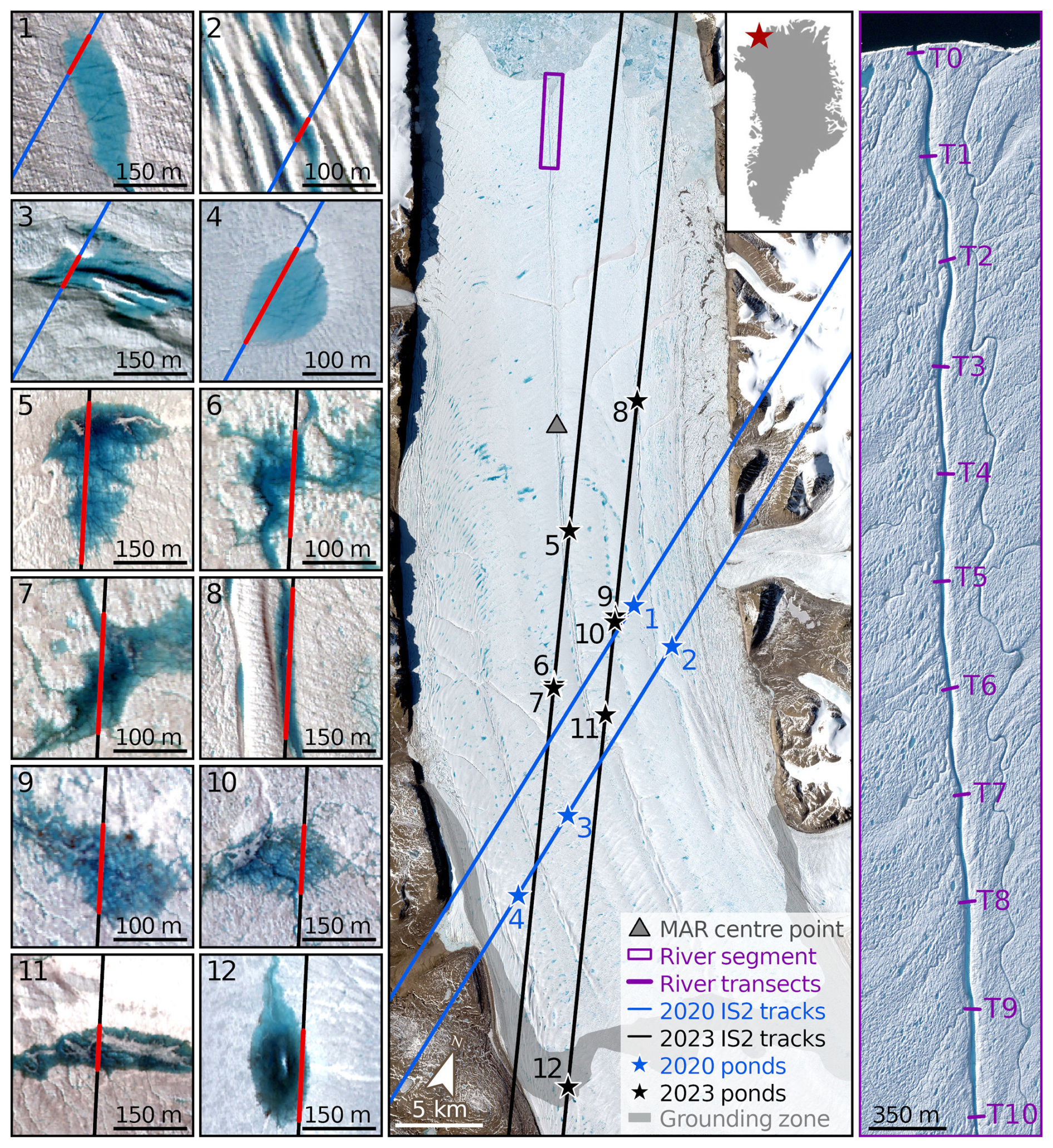
Figure 2 Sentinel-2 image of Petermann Ice Shelf from 27 June 2023, with locations of ponds, ICESat-2 beams, river segments, and grounding zone (Ciracì et al., 2023) labelled. Inset map shows the location of Petermann Ice Shelf in northwest Greenland. WorldView-2 images of ponds 1–4 (© Vantor 2020), all acquired 17 August 2020, are shown with corresponding ICESat-2 beams in blue. WorldView-2 images of ponds 5–12 (© Vantor 2023), all acquired 27 June 2023, are shown with corresponding ICESat-2 beams in black. Pond-beam intersections are shown in red. A WorldView-2 image from 12 August 2014 of the final 5 km segment of the supraglacial river (© Vantor 2014) shows the locations of the transects used in Fig. 7 in purple.

We first develop, apply, and validate our method for calculating bathymetry using a selection of ponds on the ice shelf. Focusing on ponds minimizes the need to account for large diurnal cycles in supraglacial river water levels (e.g., Smith et al., 2021; Yang et al., 2022) between WorldView-2 and ICESat-2 acquisition times and increases the number of overlaps between the two satellites over waterbodies. While some of the ponds appear to be fed and/or drained by streams, which could also cause pond water levels to fluctuate diurnally, the streams are significantly smaller than the main channel on Petermann, and thus introduce less potential error between image acquisitions. Although the river channel itself can incise depths of 8–10 m, melt season water depths observed by ICESat-2 and calculated using established optical depth algorithms (e.g., Williamson et al., 2018) are typically much shallower, ranging from 1–3 m. The water depths within the channel are therefore of a similar order of magnitude to those of the ponds used to calibrate our depth algorithm, thus we conclude that the transfer of the method from ponds to the river channel is appropriate here.

As we use ICESat-2, launched in late 2018, to validate our optical depth methods over these ponds, we consider WorldView-2/3 images collected in summers from 2019–2024. For this time period, only two pairs of WorldView-2/3 multispectral images (with corresponding DEMs) and ICESat-2 tracks have spatial overlap and were acquired within 48 h of one another over the Petermann Ice Shelf (Table S1 in the Supplement) – 17 August 2020 and 27–29 June 2023. Ponds were included in our analysis only if intersected by an ICESat-2 strong-beam track over a distance exceeding 50 m. Using these criteria, we identify 12 ponds – four in 2020 (Fig. 2, blue stars) and eight in 2023 (Fig. 2, black stars) – with a variety of depths, areas, and shapes. Two of these ponds, ponds 2 and 8 (Fig. 2), have very similar depth and geometry to the supraglacial river, which is important for calibrating the depth model for applications beyond just supraglacial ponds. Leveraging this calibration, we then apply the approach to the supraglacial river (Fig. 2) for the 2014 and 2016 melt seasons (Sect. 2.5). We pair this quantitative incision analysis with qualitative imagery analysis and modelled surface runoff data for 2013–2018 to obtain a more complete picture of the estuary formation process (Sect. 2.6). We end our analysis with the 2018 melt season as a large rift bisected the central river channel 13 km upstream of the ice front prior to the start of the 2019 melt season. As a result, the upstream portion of the river no longer reaches the open ocean, instead draining into the rift, while only the downstream portion maintains a connection to the ocean through the original estuary.

2.2 WorldView-2/3 and ArcticDEM pre-processing

WorldView-2/3 multispectral imagery is provided by the Polar Geospatial Center (PGC) in 16-bit top-of-atmosphere percent reflectance format at 1–2 m spatial resolution. The ArcticDEM strip product is also accessed through PGC and is available in 32-bit format at 1–2 m spatial resolution. Several pre-processing steps are required for both the WorldView-2/3 imagery and ArcticDEM strips prior to calculating depth and bathymetry. First, the DEMs are co-registered using the pDEMtools package in python (Chudley and Howat, 2024), with the fjord walls to the southwest of Petermann Ice Shelf as a stable reference region; the vertical error for co-registered DEMs is < 50 cm (Porter et al., 2022). To remove the influence of ice motion between acquisitions, the DEMs are manually shifted in the x and y dimensions, as required, aligning the ice-shelf front in each of the DEMs. These same x and y shifts are applied to the corresponding WorldView-2/3 images, which are then resampled to the raster grid of the DEMs using a bilinear interpolation. For the pond images, a horizontal shift in the ice flow direction is applied based on the mean ice velocity (Li et al., 2023) and the time between WorldView and ICESat-2 acquisitions (Table S1). This is done to account for any ice motion between the two data acquisitions so that the same area of ice is being compared. All selected WorldView-2/3 images (Table S1) are then radiometrically corrected using dark object subtraction (Chavez, 1996). The corrected and scaled images and DEMs are then clipped to the areas surrounding each of the 12 ponds and the 5 km of the river nearest to the ice front (Fig. 2) to increase the efficiency of our subsequent analysis.

2.3 Meltwater depth

To calculate meltwater depths of the ponds and the supraglacial river, we implement an empirical dual channel method with WorldView-2 imagery (Legleiter et al., 2014). The best fit equation is determined using optimal band ratio analysis (OBRA) with ICESat-2 derived water depths over 12 ponds (Fig. 2) as the calibration data, which we describe in detail in Sect. 2.3.3 below. This calibrated equation is then used to calculate meltwater depth, as follows:

2.3.1 WorldView-2/3 water depth calculation

First, a meltwater classification is performed using the Normalized Difference Water Index adapted for ice (NDWI_ice; Yang and Smith, 2013):

$$\begin{array}{}\text{(1)}& {\mathrm{NDWI}}_{\mathrm{ice}}={\displaystyle \frac{R_{\mathrm{B}}-R_{\mathrm{R}}}{R_{\mathrm{B}}+R_{\mathrm{R}}}},\end{array}$$

where R_B and R_R refer to the pixel reflectance in the blue and red bands of WorldView-2/3 imagery. Following Moussavi et al. (2016), a threshold of 0.23 is used for the initial meltwater classification (NDWI_ice > 0.23). Where necessary, the masks are then manually adjusted in ArcGIS Pro to omit water pixels outside of the 12 selected ponds. Subsequently, a two-pixel buffer is created at the edge of the water mask for each pond – one pixel beyond the pond edge and one pixel within the pond – to identify the water-marginal pixels. A buffer with a two-pixel width is required to account for potential errors in shoreline mapping; as the channel banks are relatively steep, a one-pixel error in shoreline location could lead to a significant error in the water surface elevation estimate, which in turn would propagate into the bathymetry calculation (Dai et al., 2018). Meltwater depth (D) is then calculated for all pixels classified as water with a dual-channel method using the logarithm of the ratio of reflectance in two bands (Legleiter et al., 2009, 2014):

$$\begin{array}{}\text{(2)}& {\displaystyle }D=a{X}^{\mathrm{2}}+bX+c,\text{(3)}& {\displaystyle }X=\ln \left({\displaystyle \frac{R_{\mathrm{1}}}{R_{\mathrm{2}}}}\right),\end{array}$$

where R₁ and R₂ are the pixel reflectances in the two selected WorldView-2/3 bands and a, b, and c are constants that are calibrated against ICESat-2 data for each WorldView-2/3 image band pair using OBRA (Sect. 2.3.3; Legleiter et al., 2009, 2014).

2.3.2 ICESat-2 calibration

To calibrate the empirical dual channel optical depth method applied to multispectral WorldView-2/3 imagery (Sect. 2.3.1), we calculate meltwater depth and basin bathymetry for our 12 selected ponds on Petermann Ice Shelf from the ICESat-2 ATL03 geolocated photon cloud product. The ICESat-2 air-water and water-ice photon returns, areas of highest photon density, must first be isolated (Fricker et al., 2020). First, all photons for which the signal confidence is “noise” or “buffer” are filtered out of the initial dataset. Then, using the scikit-learn package in Python, a Density-Based Spatial Clustering of Applications with Noise (DBSCAN; Ester et al., 1996) algorithm is used to filter out low density photons (Fig. 3a; van Leeuwen, 2023; Lv et al., 2024).

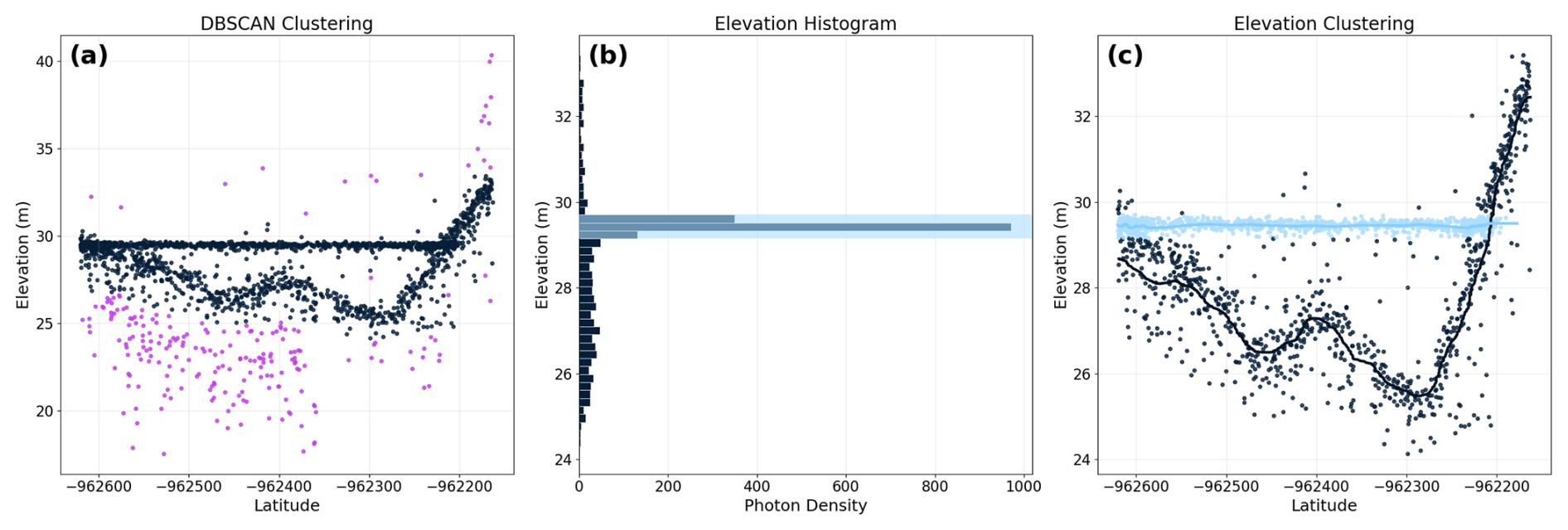
Figure 3 Example of semi-automated ICESat-2 clustering for Pond 5. Subplots show (a) DBSCAN clustering to identify low density photons (purple), which are then removed, (b) histogram of remaining, high density (navy) photon elevations with the histogram peak, indicating the water surface, highlighted in light blue, and (c) histogram-based clustering to identify the water surface (light blue) as the photons with elevations within the histogram peak in shown in (b). Moving averages are calculated through each cluster, and final clustering for all ponds can be found in Fig. S1.

With only the dense photon clusters remaining, a histogram of photon elevation can be used to isolate the water surface – the region of highest photon density by elevation and thus the histogram peak (Fig. 3b). Once the photons have been clustered by elevation, a moving average is calculated through each of the clusters to create the initial ICESat-2 water surface and ice surface profiles (Fig. 3c). A refraction correction is then applied to the ice surface profile (Datta and Wouters, 2021):

$$\begin{array}{}\text{(4)}& z_{\mathrm{bathy}}=z_{\mathrm{ice}}+\mathrm{0.25}\left(z_{\mathrm{water}}-z_{\mathrm{ice}}\right),\end{array}$$

where z_bathy is the corrected bathymetry profile, z_ice is the initial ice surface profile, and z_water is the water surface profile. Water depth is then calculated as the difference between the water surface and corrected bathymetry profiles at a given point. These calculated water depths can then be used to calibrate the empirical depth formula (Eq. 2; Sect. 2.3.3).

2.3.3 Optimal band ratio analysis (OBRA)

To calibrate the parameters in Eq. (2), we perform OBRA, following Legleiter et al. (2009), for six WorldView-2/3 multispectral bands: coastal blue (400–450 nm), blue (450–510 nm), green (510–580 nm), yellow (585–625 nm), red (630–690 nm), and red edge (705–745 nm). OBRA is a method for identifying the optimal band pair and corresponding coefficients (a, b, and c) for Eq. (2) based on the strength of the relationship between X, the log ratio of reflectances, and depth. Here, we use ICESat-2 derived water depths at corresponding points as the independent depth measurement; we then compute a regression for each of the 15 unique band combinations (Fig. 4a) to determine the quadratic best fit equation (Eqs. 2 and 3; Fig. 4). The final optimized depth-reflectance formula is the quadratic best-fit equation with the highest R² and lowest RMSE. Out of the 15 possible band combinations, our analysis shows that the optimal combination over Petermann Ice Shelf is blue (450–510 nm) and yellow (585–625 nm; R² = 0.75, RMSE = 0.29 m; Fig. 4a). Therefore, the optimised WorldView-2/3 depth-reflectance dual channel equation over Petermann Ice Shelf is:

$$\begin{array}{}\text{(5)}& D=\mathrm{1.951}\ln {\left({\displaystyle \frac{R_{\mathrm{B}}}{R_{\mathrm{y}}}}\right)}^{\mathrm{2}}+\mathrm{0.315}\ln \left({\displaystyle \frac{R_{\mathrm{B}}}{R_{\mathrm{y}}}}\right)+\mathrm{0.191},\end{array}$$

where D is depth in metres and R_B and R_Y are the WorldView-2/3 reflectances in the blue and yellow bands (Fig. 4b).

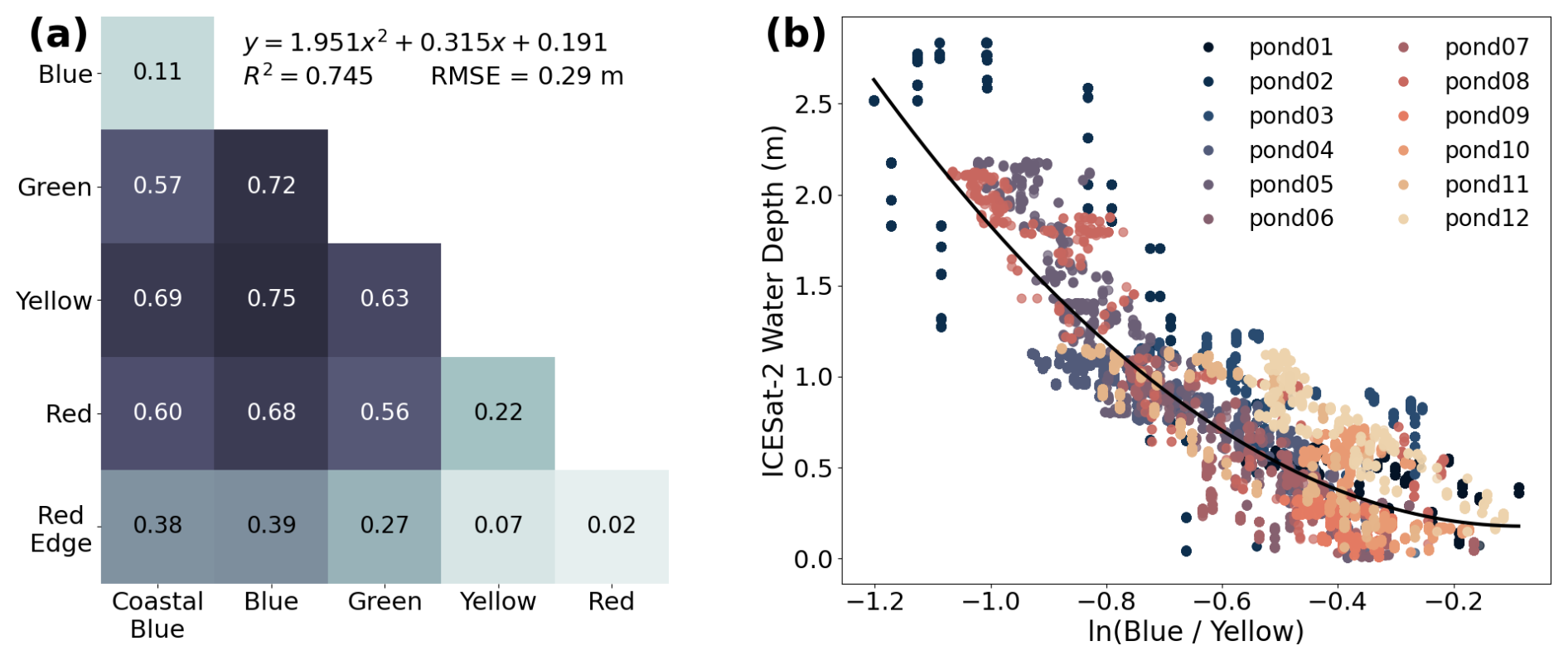
Figure 4 Dual channel depth equation calibration using OBRA: (a) heatmap showing R² for all 15 WorldView-2/3 band combinations with best fit equation and (b) scatterplot of ICESat-2 derived depths plotted against reflectance in the optimal band combination, blue and yellow, with the best fit line.

2.4 Bathymetry

Having calculated water depth from WorldView-2/3 imagery using our optimized equation (Eq. 5; Fig. S2), we calculate bathymetry. This is done by first identifying the elevation of the water surface (e.g., Dai et al., 2018) in the ArcticDEM strip product (Porter et al., 2022) corresponding to each WorldView-2/3 image, smoothing this water surface around a horizontal plane, and from this, subtracting the previously calculated water depth (Sect. 2.3).

Water surface returns in the ArcticDEM strip product are variable, sometimes appearing smooth and other times mirroring the basin or channel bathymetry (e.g. Fig. 5e). Thus, to standardize the water surface identification process for each pond, the elevation of all pixels identified as water are smoothed to equal the mean elevation of all the water-marginal pixels, yielding a flat horizontal water surface (Fig. 5a, b). The use of the mean elevation of all water-marginal pixels around the entire lake shoreline, rather than just the elevations at the endpoints of the ICESat-2 transect, is intended to mitigate any potential error introduced by elevation differences around the lake perimeter. The calculated water depths (Sect. 2.3; Fig. 5c) are subtracted from this smoothed DEM surface (Fig. 5b) to determine pond bathymetry (Fig. 5d, e). For the river, a surface elevation gradient is calculated using a linear fit to the water-marginal pixel elevation along both sides of the channel; the water surface elevation is then smoothed using this gradient (Figs. S4, S5). To calculate river channel bathymetry, the water depth is subtracted from this smoothed DEM surface. In the portion of the channel closest to the ice front, where the estuary is sometimes present, we acknowledge that the mixture of fresh and saline water may influence optical depth retrievals. However, given the relatively shallow water depths in the channel (1–3 m) and the knowledge that the influence of salinity-driven scattering in the visible wavelength bands used here is limited, we expect this effect to be small (Zhang and Hu, 2021).

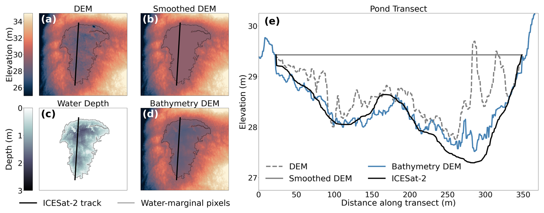
Figure 5 Example of bathymetry calculation for Pond 5. Subplots show (a) original WorldView DEM (Porter et al., 2022) with water-marginal pixels in grey and ICESat-2 transect location in black, (b) Smoothed DEM with water surface set equal to mean water-marginal pixel elevation, and (c) meltwater depth calculated from WorldView-2 imagery, (d) Bathymetry DEM, equal to smoothed DEM surface minus water depth, and (e) elevation profiles along the ICESat-2 transect. Examples of bathymetry calculation for all ponds can be found in Fig. S3.

2.5 Supraglacial river incision rate

2.5.1 Tidal correction

To calculate the incision rate of the Petermann Ice Shelf supraglacial river, the DEMs must be tidally corrected (Figs. S6, S7). At Petermann, the tidal range is approximately 2 m, and the ice shelf oscillates relatively freely with the ambient tide from at least 26 km downstream of the grounding zone (Münchow et al., 2016). We run the Greenland 1 km Tide Model (Gr1kmTM; Howard and Padman, 2021) to calculate an elevation correction for each of the DEMs based on the acquisition dates and times (Figs. S6, S7; Table S1). The open ocean surface elevation, often obscured by either sea ice or clouds, yields highly variable, unreliable surface elevations (e.g., Fig. S8). Thus, to estimate sea level elevation for each corrected ArcticDEM strip, we use the mean elevation of the seawater surface along the margins of two rifts near the ice-shelf front (similar to mean marginal pixel elevation in Sect. 2.4); this is done for all of the images with open water. We then calculate a mean sea surface elevation for each melt season, which we set to 0 m in each of the tidally-corrected DEM strips (Figs. S6, S7).

2.5.2 Incision rate calculation

Focussing our incision rate calculations on the 5 km of the supraglacial river closest to the ice front, we prescribe 11, 70 m-wide transects, perpendicular to the river centreline and evenly spaced every 500 m (Fig. 2). If necessary, these transects are manually shifted 1–2 pixels along the river centreline to minimize overlap with shaded pixels and floating sea ice. By extracting bathymetry along these transects for five dates in each of the 2014 and 2016 melt seasons, we calculate incision rate (I) as the change in channel bottom elevation over time:

$$\begin{array}{}\text{(6)}& I={\displaystyle \frac{\mathrm{\Delta }{z}_{\mathrm{bathy}}}{\mathrm{\Delta }t}},\end{array}$$

Where Δz_bathy is the change in channel bottom elevation in metres and Δt is change in time in days.

We also calculate the incision rate as a continuous profile along a manually-delineated river centreline. As with the transects, this profile deviates 1–2 pixels from the centre of the river in some locations to minimize overlap with shaded pixels and floating sea ice. For comparison with this along-channel incision rate, surface ablation rate is also calculated as the difference in ice-shelf surface elevation over time along a longitudinal surface transect to the west of the river. These along-river and surface elevation profiles are then smoothed with a 1-pixel buffer, which considers all the surrounding pixels, before being used to calculate incision and surface ablation rates.

2.6 Estuary formation timeline analysis

To constrain the timeline of estuary formation, we analyse our calculated incision rates (Sect. 2.5.2) in the context of meltwater runoff data from the Modèle Atmosphérique Régional (MAR) and visually analysed WorldView-2/3 multispectral imagery, as follows:

2.6.1 Runoff data

We use output from the regional climate model MAR, version 3.11 (Fettweis and Grailet, 2024), to analyse trends in surface meltwater runoff over the Petermann Ice Shelf for 2013–2018; the time period when WorldView-2/3 multispectral imagery is available and before a transverse ice-shelf fracture intersected the supraglacial river (2018), disrupting the hydrologic connectivity of the surface drainage network. We use MAR's meltwater runoff variable from the daily gridded 10 km product, extracted at a central point on Petermann Ice Shelf (Fig. 2).

2.6.2 Qualitative imagery analysis

We also visually analyse 22 WorldView-2/3 multispectral images acquired over the Petermann Ice Shelf estuary from 2013–2018. Ten of these images are those from 2014 and 2016 that are also used in the river incision analysis (Sect. 2.5.2), and the remaining 12 include all cloud-free multispectral images available over the estuary in summer 2013, 2015, 2017, and 2018 (Table S1). The four criteria considered to indicate the true presence of an estuary are: (1) visible connection of the water surface between the supraglacial river and ocean, (2) convergent sea ice at the mouth of the river, (3) presence of sea ice within the river channel, and/or (4) presence of seawater in the channel after the melt season ends (Boghosian et al., 2021). Images that clearly do not meet any of these criteria are classified as “no estuary”, and ambiguous images where at least one of the criteria may be met are classified as “potential estuary”. Images that definitively meet at least one of the criteria are classified as “estuary”, and those that meet more than one criterion are classified as “confirmed estuary”.

3 Results

3.1 Supraglacial river incision

3.1.1 Along-channel incision

Mean incision rates along the centreline of the 5 km segment of the Petermann channel for the 2014 and 2016 melt seasons are 3.0 ± 0.44 and 2.9 ± 0.34 cm d⁻¹, respectively. In total, 1.8 ± 0.27 m incision occurs over 61 d (20 June–18 August) in 2014, while 1.7 ± 0.20 m incision occurs over 59 d (15 June–15 August) in 2016. For both years, the last available images showing water along the full channel were acquired mid to late August, 1–2 weeks before the end of the melt season, meaning incision for each melt season is likely a slight underestimate. Despite similar mean incision rates over these two melt seasons, the spatial patterns of incision along the river channel vary significantly between the two melt seasons. During the 2014 melt season, the greatest incision rate is localized in the kilometre of the channel closest to the ice front (0–1 km in Fig. 6a, c), reaching a maximum of 4.0 cm d⁻¹. Moving upstream of the ice-shelf front, the 2014 incision rate decreases until ∼ 2 km (1–2 km in Fig. 6a, c), from which point it remains at ∼ 2.7 cm d⁻¹ until 5 km upstream (2–5 km in Fig. 6a, c). In contrast, during the 2016 melt season, the incision rate is lowest closest to the ice front (2.2 cm d⁻¹ from 0–1 km in Fig. 6b, c) and then increases over the next kilometre (1–2 km in Fig. 6b, c), before levelling out at ∼ 2.9 cm d⁻¹ for the final 3 km (2–5 km in Fig. 6b, c). During both melt seasons, the early season ice front channel-bottom elevation is above sea level, at 2.6 m on 20 June 2014 and 1.5 m on 15 June 2016 (dark blue lines, Fig. 6), dropping below sea level by mid-August in 2014 and mid-July in 2016 (light green lines, Fig. 6).

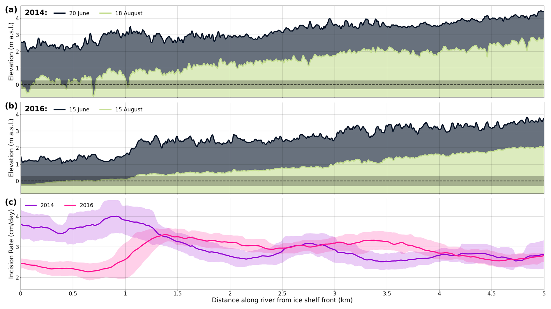
Figure 6 Supraglacial river/estuary tidally corrected channel-bottom elevation profiles from June (dark blue) and August (light green) during the (a) 2014 and (b) 2016 melt seasons; mean sea level is shown as a dashed black line with 1σ shaded. Panel (c) shows corresponding along-channel mean incision rates for 2014 and 2016 with 1σ shaded.

3.1.2 Cross-section incision

We also consider cross-sectional incision profiles (Fig. 7) at 11 transects along the supraglacial channel (Fig. 2). For 2014, incision across all transects is primarily vertically downward (Fig. 7a). In contrast, in 2016, many of the transects exhibit both vertical and lateral incision, widening and flattening the channel floor (Fig. 7b). Between the 2014 and 2016 melt seasons, the channel widens at all transects, especially near the ice-shelf front (transects 0–3). The channel widens from a mean of 20 m in 2014 to 25 m in 2016. In 2014, peak incision occurs between 6 July and 12 August, as shown by the channel deepening significantly along the entire length of the river (Fig. 7a). In contrast, in 2016, the peak incision occurs earlier in the melt season, between 20 June and 13 July, with minimal change between 13 July and 15 August (Fig. 7b).

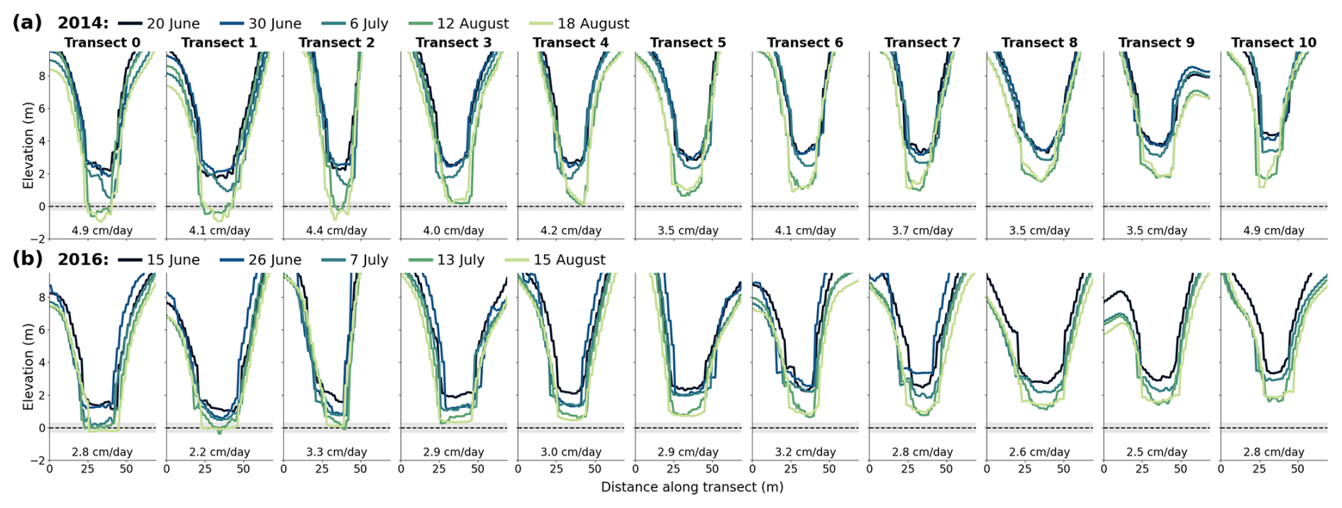
Figure 7 Channel bathymetry cross-sections and vertical incision rates at 11 transects along the supraglacial river (Transect 0 is at the ice-shelf front and Transect 10 is 5 km upstream of the ice front; see Fig. 2 for exact transect locations) throughout the (a) 2014 and (b) 2016 melt seasons. At each transect and in each melt season, cross section bathymetry (m above sea level) is shown for five dates, in five discrete colours; mean sea level is shown as a dashed black line with 1σ shaded. The mean (mid-June to mid-August) incision rate at each transect is stated in black text at the bottom of each sub plot.

3.2 Petermann estuary formation timeline

To complement our incision rate results in Sect. 3.1, in order to better constrain the timeline of estuary formation, we consider surface runoff data extracted from MAR alongside qualitative interpretation of multispectral WorldView-2/3 imagery of the river/estuary from 2013 to 2018. During the 2013 melt season, no conclusive visual evidence (Sect. 2.6.2) of an estuary is observed (Fig. 8a, b), and the MAR data indicates 2013 has the lowest annual runoff for the period 2013–2018 (Fig. 8). The early 2014 melt season images prior to peak runoff – 20 June (Fig. 8c), 30 June and 6 July – also show no indication of estuary presence. After peak runoff, the 12 August (Fig. 8d) and 18 August images appear to have a continuous water surface from the ocean into the channel, as well as darker coloured, deeper water within the mouth of the channel, indicating that an estuary may have formed. An image from 1 September 2014 (Fig. 8e) with seawater in the channel after the melt season confirms the presence of the estuary by this date. Only one image was collected during the 2015 melt season, on 10 July (Fig. 8f), just after peak runoff. This image may show convergent sea ice near the mouth of the channel, an indication of estuary presence, or a residual winter sea ice blockage. The first image from the 2016 melt season, on 15 June, has no estuary indicators due to the partial sea ice blockage (Fig. 8g), but by 26 June, there is some evidence of estuary formation. After 7 July 2016, all available images in the remainder of this melt season indicate that an estuary has formed (e.g., Fig. 8h). In 2017, an image from 6 June shows a partially filled river channel with a sea ice blockage at the front; the blockage dissipates sometime between 30 June and 26 July, after which an estuary is once again present. Both images from the 2018 melt season indicate estuary persistence (Fig. 8k, l), but there are no early melt season images to determine whether the channel was temporarily disconnected from the ocean. In summary, the Petermann estuary appears to be ephemeral, in most years forming in late July and persisting through the end of the melt season, before becoming disconnected from the ocean between melt seasons.

For 2014 and 2016 – the two melt seasons for which we calculate incision rates (Sect. 3.1) – the total modelled surface runoff from MAR is very similar between the years, 936 mm water equivalent (w.e.) and 975 mm w.e. respectively, with peak runoff occurring on 22 July in 2014 and 20 July in 2016 (Fig. 8). When we estimate ice-shelf surface ablation by differencing our tidally-corrected DEMs along a surface transect to the west of the river, we also find close similarity between the two years; 1.4 ± 0.4 m in 2014 (0.25 ± 0.07 mm d⁻¹) and 1.4 ± 0.3 m in 2016 (0.24 ± 0.05 mm d⁻¹). It should be noted that these are likely overestimates as they do not account for hydrostatic adjustment due to basal melt; nevertheless, the 2016 estimate agrees well with in-situ observations of surface melt on Petermann Ice Shelf (1.4 ± 0.2 m) from Washam et al. (2019) over a similar time period. While the MAR and DEM-differencing estimates are not directly comparable due to their differing spatial and temporal domains, both methods indicate that there is close similarity in the magnitude of surface melt and runoff between the two years.

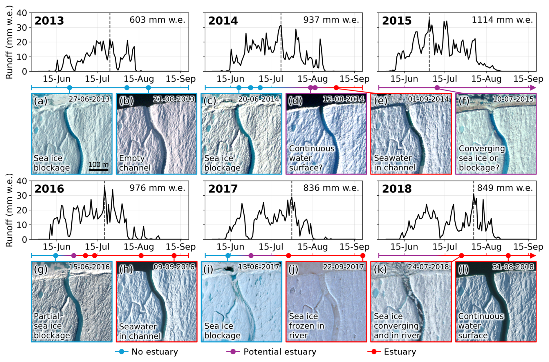
Figure 8 Timeline of Petermann Ice Shelf estuary formation showing surface runoff and WorldView imagery from 2013 to 2018 (© Vantor 2025). Summer (1 June to 15 September) runoff over Petermann Ice Shelf from MAR is shown in black with a dashed line indicating peak runoff. A corresponding timeline coloured by likelihood of estuary presence (blue for no estuary, purple for ambiguous, and red for estuary) is shown below each of the runoff plots with coloured circles on the timeline representing availability of cloud-free WorldView-2/3 images; 12 example images (a–l; all at the same spatial scale) are shown below their respective coloured circles on the timeline and are labelled with relevant estuary formation criteria information. Gradients between two solid colours on the timeline indicate that a change in estuary likelihood occurred between two dates, but that the exact timing cannot be determined. At the end of each melt season, it is assumed that the conditions from the last cloud free image persist until refreezing. Additional images used to develop the timeline but not shown here can be found in Fig. S9.

We note that there may not always be perfect agreement between the channel bottom elevation relative to mean sea level (Figs. 6, 7) and the visual indicators of estuary presence in the WorldView imagery (Fig. 8). This is because diurnal tidal fluctuations, wind, and waves can cause seawater to enter the channel once the channel bottom elevation is close to, but not necessarily below, mean sea level, and because our mean sea level estimate carries some uncertainty (Figs. 6, 7). Therefore, the elevation threshold above mean sea-level at which seawater can first enter the channel is not precisely known, and visual indicators of estuary presence in WorldView imagery may precede the date when the channel bottom drops definitively below mean sea-level in our elevation profiles (Figs. 6, 7).

4 Discussion

4.1 Evolution of the Petermann Ice Shelf estuary

To better understand the process of estuary formation on the Petermann Ice Shelf, we discuss the results of our various analyses together, namely satellite remotely-sensed incision rates, visual interpretations from optical satellite imagery, and modelled ice-shelf runoff data.

Calculated incision rates vary in magnitude over space and through time but fall within the reasonable range of supraglacial incision rates (2–6 cm d⁻¹) identified by Pitcher and Smith (2019) for the Greenland Ice Sheet. However, there are key differences in the melt patterns between the 2014 and 2016 melt seasons. In 2014, the along-channel vertical incision rate is highest near the front of the ice shelf, reaching a maximum of 4.0 cm d⁻¹, and decreases moving upstream from the ice front (Fig. 6a). In 2016, this pattern is reversed, with the lowest along-channel vertical incision rates occurring near the ice-shelf front; 2.2 cm d⁻¹ within the first kilometre and increasing with distance away from the ice-shelf front (Fig. 6b). Crucially, we note that these differences in incision rates are observed despite strong similarity in total melt volume for 2014 and 2016, with peak runoff also occurring only two days apart, 22 July vs. 20 July, respectively (Fig. 8). Variation in meltwater production is therefore unlikely to explain the observed differences in incision rates between the two years. The slightly steeper slope of the channel bottom at the end of the 2014 melt season (Fig. 6a) compared to the 2016 melt season (Fig. 6b) could contribute to faster river flow and thus increased vertical incision (Holland and Jenkins, 1999). However, the mean slope over the 5 km river segment for both melt seasons is 0.03° (Fig. 6a–b), therefore it is unlikely that this is a major driver of the overall slightly higher mean incision rates observed in 2014 compared to 2016. Furthermore, surface slope varies gradually and consistently over the full 5 km study reach on all observed dates in both years (Fig. 6a–b) and therefore cannot explain why the most pronounced differences in incision rate between 2014 and 2016 are confined to the 1.5 km nearest the ice-shelf front (Fig. 6c).

From our analysis of incision rates across transects every 500 m up the river channel, we also observe that, in 2014, the bathymetry of the river channel appears to remain relatively narrow throughout the melt season (Fig. 7a), indicative of vertical incision dominating (Fig. 9a). Whereas in 2016, the channel is generally wider and flatter, particularly in the kilometre of the channel closest to the ice front (Fig. 7b), indicative of lateral erosion dominating (Fig. 9b). This pattern of widening has also been noted for the entire 2013–2018 period and is most pronounced closest to the ice-shelf front (Boghosian et al., 2021). These observations, along with those described in the paragraph above, are consistent with the estuary being absent for most of the 2014 melt season, and present for the majority of the 2016 melt season.

Once an ice-shelf estuary has formed, we would expect the vertical incision rate near the ice front to decline and the channel morphometry to become wider and flatter (Fig. 9b). The reasons for these changes in incision rates and channel morphology are two-fold. First, channel melting is controlled by turbulent heat exchange at the ice-water boundary, driven by both the heat content of the water and the flow speed (Holland and Jenkins, 1999). During the river phase, fast unidirectional flow concentrates melt at the bottom of the channel, favoring vertical incision (Pitcher and Smith, 2019). Once the estuary forms and tidal flow reversal begins, the net seaward flow speed is reduced, lowering the turbulent exchange velocity and thus the rate of vertical incision. Second, the intrusion of warm, saline seawater increases thermally driven melt, and the shear between the two converging water masses drives melting more broadly across the channel walls rather than concentrating it at the channel bed (Boghosian et al., 2021; Holland and Jenkins, 1999). Additionally, as in terrestrial estuaries, the two water masses may not mix instantaneously but instead form a stratified system, with less dense freshwater flowing seaward above denser inflowing seawater, further distributing melt across the channel profile rather than concentrating it along the centre of the bed (Geyer and MacCready, 2014). Although the relative melt contributions of seawater and supraglacial meltwater depend on their respective temperatures and flow speeds, which are not known here, we hypothesize that the net effect of estuary formation is to shift the dominant melt pattern from vertical incision to lateral erosion, causing the channel to become broader and flatter rather than narrower and deeper. This is consistent with our cross-sectional observations of the channel, which show widening and flattening of the channel that is most pronounced in the 1.5 km nearest the ice-shelf front (Fig. 7b).

However, we suggest that the story is more complicated than described above, as the estuary did not persist continuously throughout our analysis timeline. Even as early as 2014, we see evidence of estuary formation toward the end of the melt season, shortly after incision rates peak (July–August), when the channel bottom elevation drops below sea level (Figs. 6, 7). Additional evidence for this comes from an August 2014 WorldView image (Fig. 8d), which appears to show a continuous water surface between the river and ocean, and a September 2014 image (Fig. 8e) which shows water in only the mouth of the river channel after the MAR runoff data indicates that melting has ceased. Following Boghosian et al. (2021), we interpret this residual water as seawater, indicating the presence of a persistent estuary at the start of September 2014, after the melt season has ended.

At the start of the 2016 melt season, however, no estuary is documented as the channel bottom is no longer below sea level (Figs. 6b, 7b). Hydrostatic uplift of the ice shelf in response to meltwater unloading in the latter parts of the previous melt season, may have elevated the channel bottom above sea level (e.g., Banwell et al., 2019). The timescale of this flexural rebound is not well constrained, and it is likely that seawater continues to flow into the channel with the tide for some period after surface melting ceases before eventually freezing in-situ, with this refreezing potentially contributing an additional, though unquantified, rise of the channel bottom elevation above sea level. Additionally, ice flow perpendicular to the central basal channel, known as secondary flow, likely also contributes to this elevation of the surface channel above sea level by thickening the ice between the surface and basal channels (Wearing et al., 2021). We also observe a partial sea ice blockage at the mouth of the estuary in mid-June 2016 (Fig. 8g), which may have reduced river-water/ocean-water interactions at the ice-shelf front. By early July 2016, the observed incision rates peak (June–July), the blockage is no longer present, and the channel bottom is once again below sea level (Fig. 7b). Images from 7 and 13 July show sea ice floating in the river channel and converging at the mouth of the channel, a clear indicator of water flow reversal and estuary presence (Boghosian et al., 2021). From July until late September 2016, we observe widening of the channel, particularly near the ice-shelf front (Fig. 7b), which as described above, is also indicative of estuary presence. As with 2014, meltwater persists in the river channel after the melt season has ended (Fig. 8h).

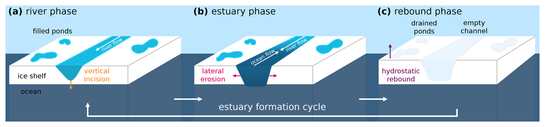
Figure 9 Schematic of the proposed estuary formation cycle. During the early melt season, the channel is in its river phase (a), where meltwater is exported from the ice shelf into the ocean through river flow, causing the river to incise vertically into the ice-shelf surface. Once the river incises to the point where the channel bottom reaches sea level, the estuary phase (b) begins. During this phase, meltwater export from the ice shelf is limited by mixing with seawater, leading to flow reversal in the lower part of the river channel, with seawater flowing up the channel. In this phase, lateral erosion rather than vertical incision dominates, causing the channel to widen. The rebound phase (c) occurs towards the end of the melt season as surface melting ceases and meltwater is offloaded from the ice-shelf surface, causing the most downstream part of the ice shelf to hydrostatically flex upwards, thereby raising the channel bottom above sea level; refreezing of seawater in the river channel likely also contributes to elevating the channel bottom above sea level. After surface melting has initiated in the subsequent summer, the river may start to flow again, and the estuary formation process recommences.

Given that our observations show that the estuary is present at the end of the 2014 melt season but not at the start of the 2016 melt season, we suggest that the estuary forms repeatedly with the channel becoming seasonally disconnected from the ocean (Fig. 9) by ice-shelf uplift, refreezing of seawater in the channel, and/or sea ice blockage. The estuary could have formed prior to the 2014 melt season, as well as during the 2015 season but was not resolved; due to the limited availability of WorldView imagery in 2013 and 2015, this is inconclusive. In 2017, images from the beginning of the melt season indicate that the river has once again become disconnected from the ocean (Fig. 8i), and by the end of July, the estuary has formed once again persisting through the end of the melt season (Fig. 8j). Both available images from the 2018 melt season (24 July and 31 August; Fig. 8k, l) show evidence of estuary presence, but there is insufficient early melt season imagery to determine whether the estuary is again disconnected during this time. We do not extend our imagery analysis beyond 2018 due to the appearance of a rift upstream of the ice front that intersects with the river channel; the upstream portion of the river now drains into this rift rather than the ocean.

For 2014 to 2018, the Petermann estuary likely occupies only the final few kilometres of the ice shelf, a region that has been shown to contribute little to buttressing of upstream glacier flow (Rückamp et al., 2019). However, as Boghosian et al. (2021) demonstrate, estuary formation on Petermann Ice Shelf has already been associated with the development of longitudinal fractures that propagate upstream from the calving front, promoting transverse fractures which sometimes lead to rectilinear calving events. For example, the formation of the 2018 rift was likely driven by the combined influence of estuarine weakening and concentrated ice-shelf thinning along the central basal channel (Dow et al., 2018). Further, these processes likely contributed to a large rectilinear calving event (∼ 75 km²) along this rift on 4 August 2026, as observed in Sentinel-1 radar imagery, suggesting that even the spatially and temporally limited seawater intrusion documented here prior to 2018 may have been sufficient to weaken the ice shelf and contribute to fracturing. If continued channel melting driven by warm seawater intrusion thins the ice shelf and lowers the freeboard in the channel, seawater may penetrate further upstream towards the grounding zone, allowing estuarine-induced flexural weakening to influence ice that plays a more significant buttressing role. It is worth noting, however, that the conditions required for estuary formation – low freeboard and high surface melt – also promote ice-shelf instability through surface meltwater ponding and hydrofracture (e.g., Banwell, 2017), meaning that by the time an estuary forms, the ice shelf may already be significantly weakened. Estuary formation may therefore represent one of several concurrent destabilizing processes on an already-vulnerable ice shelf, rather than a singular potential trigger for collapse.

The discussion above suggests that spatial and temporal variations in river channel incision rate can be strong indicators of estuary formation. Estimating incision rates along a channel may help to inform us about when and where estuaries could form in the future. However, as alluded to in the paragraph above, incision rate is likely not the only driver of estuary formation. Estuary formation depends also on other factors, particularly ice-shelf freeboard – the height of ice above floatation – and basal channel depth (Glazer et al., 2024). For the Petermann Ice Shelf, freeboard is generally less than 10 m – similar to the freeboard of the Ryder and 79N ice shelves in Greenland, both of which are also known to have large basal channels (e.g., Song et al., 2022). The large central river on Ryder reaches the ice-shelf front, and there is some evidence of estuary formation within the past decade (Boghosian et al., 2021). The river on 79N does not yet reach the ocean, however, due to the low freeboard and presence of basal channels, there is potential for an estuary to form if a calving event connects the surface river with the ocean. On Petermann, the upstream portion of the river could itself form a new estuary at the 2018 rift location in the coming years, particularly as the ice shelf downstream of the rift calved rectilinearly on 4 August 2026, as seen in Sentinel-1 radar imagery, connecting the river to the ocean. For many Antarctic ice shelves, freeboard can be upwards of 20 m (e.g., Chartrand and Howat, 2023; Griggs and Bamber, 2011). Therefore, future work could focus on further refining first-order estimates of how long it would take for estuaries to form on ice shelves with known thickness and initial surface channel depth, often controlled by the basal channel depth, based on calculated incision rates using the methods described here and estimates of melt season duration.

4.2 Bathymetry methodology applications and limitations

The novel method presented here for using paired WorldView imagery and corresponding DEMs to calculate meltwater depth and bathymetry performs best using the blue and yellow band combination when compared to ICESat-2 derived depth and bathymetry data (R² = 0.75, RMSE = 0.29 m, Bias = +0.01 m; Fig. 4). While we find that the dual channel model with the blue and yellow band combination performs best over Petermann Ice Shelf, Legleiter et al. (2014) find that the coastal blue and green band combination performs best over a region in southwestern Greenland (R² = 0.92, RMSE = 0.49 m), and Moussavi et al. (2016) find that the blue and green band combination performs best over a region in western Greenland (R² = 0.99, RMSE = 0.41 m). The inclusion of the yellow band in our best fit equation may be due to the predominantly shallow to intermediate depth (1–3 m) waterbodies on the Petermann Ice Shelf, as the yellow band's penetration depth through water falls between the red – best for shallow water – and green – best for deep water – bands (Lutz et al., 2024; Melling et al., 2024; Williamson et al., 2018). These varying results between studies and locations emphasize the importance of study site-specific model calibration to yield the most accurate water depth results.

Although we utilize a dual channel optical model (Legleiter et al., 2009) for calculating supraglacial water depth, there are many other reflectance-based depth models that could instead be implemented in conjunction with the ArcticDEM strip product to calculate bathymetry. Of these models, many have been developed or adapted for use with WorldView imagery (e.g., Legleiter et al., 2014; Moussavi et al., 2016) and could thus be implemented directly. Additional methods developed for other sensors such as Landsat and Sentinel-2 (e.g., Lutz et al., 2024; Williamson et al., 2018) may require additional calibration for use with WorldView imagery prior to being implemented with this methodology. When used to calculate incision rate, as in this study, this methodology could provide additional insights into supraglacial river processes such as the ability of enhanced river incision to promote transverse fracture (Dow et al., 2018). Further, it could be used to constrain channel geometry for estimates of meltwater export through a surface rivers in order to assess their ability to mitigate instability (Bell et al., 2017).

The main limitation of the approach presented here is data availability, as it requires corresponding WorldView imagery and ArcticDEM strips, which are not consistently available over many locations in the Arctic and Antarctic. Furthermore, even when such data are available, it provides only a snapshot in time, so we are unable to resolve sub-daily scale processes such as diurnal water level fluctuations. A further limitation is that WorldView imagery is not openly available, with access requiring either a commercial license or provision via a federally funded grant and organizations such as the Polar Geospatial Center. This represents a practical constraint on the wider adoption of the methods presented here; future work could explore whether similar approaches could be developed using freely available satellite data, such as Sentinel-2 or Landsat 8/9 imagery, albeit at coarser spatial resolution.

For the meltwater depth component, shadows present a challenge for accurate retrieval, as shaded pixels often result in artificially deep depths due to their spectral characteristics. This is particularly notable at high latitudes, where the high solar zenith angle at the beginning and end of the melt season can cast long shadows through most of the day. To mitigate the influence of shadows on our analysis, transects and river profiles are drawn to avoid shaded pixels whenever possible. For ice-shelf estuaries, higher salinity closer to the ice front may reduce depth retrieval accuracy. However, the shallow water depths (1–3 m) and the limited sensitivity of visible-band reflectance to salinity-driven scattering (Zhang and Hu, 2021), means that this effect is likely to be a minor source of uncertainty. The implications of this scattering could be better assessed and characterized with field measurements, data which could also be used to validate the incision calculations presented here. Furthermore, as the volume of seawater intruding into the channel, its reach within the river/estuary, and the magnitude to which it limits meltwater export remain poorly constrained, direct measurements of water temperature, salinity, and flow velocity would help to fully assess the impact of the estuary on ice-shelf stability.

5 Conclusions

Supraglacial rivers on ice shelves may mitigate ice-shelf instability by draining meltwater to the ocean that would otherwise pond on the surface (Bell et al., 2017). However, the evolution of a river into an ice-shelf estuary may counteract this effect by limiting efficient meltwater export and allowing up-ice intrusion of warmer, saline seawater (Boghosian et al., 2021), thereby shifting the dominant melt pattern in the channel from vertical incision to lateral erosion, and loading the ice shelf with both meltwater and seawater. We investigate the timeline and dynamics of estuary formation on Petermann Ice Shelf between 2013 and 2018 through quantitative analysis of satellite remotely-sensed channel bathymetry and incision rate alongside modelled surface runoff and qualitative visual analysis of imagery. We calculate incision using a dual channel optical depth method applied to WorldView imagery and referenced to corresponding DEMs. This novel method provides a valuable tool for calculating bathymetry and incision rate where ICESat-2 coverage is limited. When applied to Petermann's supraglacial river, our method reveals significant spatial and temporal variability in incision rates between 2014 and 2016, which we interpret as being indicative of the cyclical formation process of the Petermann Ice Shelf estuary. Qualitative imagery analysis provides further insight into the dynamics of estuary formation, revealing that the river channel becomes seasonally disconnected from the ocean and the estuary re-forms during each subsequent melt season until 2018, when a large rift bisects the river channel 14 km upstream of the ice front. We attribute the formation of this rift to the combined influence of estuarine weakening and concentrated ice-shelf thinning along the basal channel. This indicates that estuary presence, even when spatially and temporally limited, can weaken the ice shelf substantially enough to drive fracture, and calving, and will thus likely become increasingly important as the Earth warms. When combined with forward models – initialized with observations of other drivers of estuary formation, including ice-shelf thickness, basal channel depth, and basal and surface melt – this approach would improve our understanding of how estuary formation affects long-term ice-shelf stability, as well as where and when future ice-shelf estuaries may develop in Greenland and Antarctica.