Evaluation of meltwater-over-accumulation ratio as a predictor of surface ponding on Antarctic ice shelves

Ponding of surface meltwater on Antarctic Peninsula ice shelves has led to hydrofracture-driven calving and grounding line retreat, and other regions could become vulnerable to increased ponding as the climate continues to warm. Theory and qualitative observations suggest that ponding initiates when the meltwater-over-accumulation ratio (MOA) reaches 0.7. Here, we use present-day satellite-derived Antarctic meltwater products and RACMO climate model outputs to calibrate predictive thresholds of surface ponding based on air temperature, MOA, and a weighted combination of MOA and a grounding line proximity index (GLPI).

We tested three RACMO resolutions (27, 11, and 2 km) and three surface meltwater products. The meltwater product that is best aligned with MOA identifies ponding locations using aggregate meltwater depths at 27 km resolution. For this product, the calibrated MOA and GLPI threshold predicts present-day ponding with an F1 score over twice as high as the theoretical threshold of MOA ≥ 0.7 (F1 = 0.587 vs. 0.261). Under emissions pathway SSP1-2.6, the empirical threshold predicts 2.3 times more lake coverage by 2100 than the theoretical threshold, underscoring the importance of calibrating climatic ponding thresholds. If MOA-based thresholds are to be used in future ponding projections, we recommend they be applied at relatively coarse spatial scales, calibrated against present-day, depth-based meltwater products, and combined with grounding line proximal processes.

1 Introduction

Ice shelves play an important role in mitigating sea-level rise from the Antarctic ice sheet by exerting buttressing forces against the seaward flow of inland grounded ice (Dupont and Alley, 2005; Rignot et al., 2011). This buttressing effect is complex and often nonlocal. Removing some ice shelf regions would have little to no effect on upstream ice, while removing others could accelerate upstream glaciers by up to eight times their current speed (Fürst et al., 2016). In Antarctica, ice shelves lose approximately half of their mass through iceberg calving and half through basal melting (Adusumilli et al., 2020; Depoorter et al., 2013; Smith et al., 2020), while direct surface melt runoff is negligible in terms of overall mass loss. However, surface meltwater can strongly influence the stability of ice shelves, and therefore makes an indirect, yet significant, contribution to the ice sheet's mass budget.

Surface meltwater is widespread across Antarctica, occurring mainly at the lower latitudes and altitudes of ice shelves (Stokes et al., 2019; Tuckett et al., 2025) and near areas of blue ice and exposed rocky outcrops, where albedo is lower relative to surrounding snow and ice surfaces (Kingslake et al., 2017). Ponded meltwater on ice shelves can induce hydrofracture, in which water-filled crevasses deepen and propagate through the ice under pressure. Such fracturing can weaken the ice and initiate a chain reaction of large-scale calving and rapid ice-shelf retreat (Banwell et al., 2013; Munneke et al., 2014; Scambos et al., 2000, 2003). Surface ponding is therefore implicated in observed instances of thinning and collapse. This has been observed primarily on the Antarctic Peninsula, which is rapidly warming (Turner et al., 2005) and has the most intense surface melting observed in Antarctica (Bell et al., 2018; Turner et al., 2016). For example, the Larsen A Ice Shelf  disintegrated over a few weeks in early 1995, losing ∼ 2000 km² following extensive meltwater infiltration and a series of large calving events (Rott et al., 1996). Similarly, the Larsen B Ice Shelf collapsed within days in February 2002, in an event associated with synchronized drainage of over 2750 supraglacial lakes (Banwell et al., 2013; Cook and Vaughan, 2010; MacAyeal et al., 2003; Scambos et al., 2003). While it remains unclear whether the lake drainage was a cause or a consequence of collapse (Leeson et al., 2020), extensive surface meltwater ponding is widely thought to have preconditioned the shelf for disintegration through hydrofracture.

Given the demonstrated role of surface meltwater in the collapse of Antarctic Peninsula ice shelves, and the increasing air temperatures over the Antarctic continent in recent decades (Oppenheimer et al., 2019), it is important to identify the conditions that promote surface melt accumulation continent-wide, and assess the potential for meltwater-induced instability beyond just the Peninsula. It has been proposed that a mean annual isotherm of −9 °C represents a critical threshold above which ice shelves are susceptible to a destabilizing amount of surface meltwater (Morris and Vaughan, 2003). This threshold was empirically confirmed on the Peninsula, where Cook and Vaughan (2010) noted that seven of the twelve ice shelves have retreated significantly or entirely disintegrated since the mid-twentieth century, following a southerly migrating thermal boundary. However, when expanding to other regions of the continent, temperature alone cannot reliably predict ponding locations (van Wessem et al., 2023). Meltwater only accumulates where the surface and near-surface ice are impermeable due to firn compaction or refreezing of meltwater within the ice column. Otherwise, surface melt can percolate englacially into the firn air space instead of ponding (Kingslake et al., 2017; Lenaerts et al., 2017; Munneke et al., 2014). It is estimated that 94 % to 96 % of surface melt in Antarctica is retained or refrozen within the underlying firn (van Wessem et al., 2018; Veldhuijsen et al., 2024).

Depletion of firn air space occurs most efficiently in regions with high melt production and low snowfall (Bevan et al., 2017; Munneke et al., 2014). Therefore, the average melt-over-accumulation ratio (MOA) is theorized to be a stronger predictor of surface ponding than temperature alone (Pfeffer et al., 1991; van Wessem et al., 2023). MOA is calculated as the ratio of annual average liquid water production to snow accumulation as follows:

$$\begin{array}{}\text{(1)}& \mathrm{MOA}={\displaystyle \frac{\mathrm{melt}}{\mathrm{accumulation}}}={\displaystyle \frac{\mathrm{snowmelt}+\mathrm{rain}}{\mathrm{snowfall}-\mathrm{sublimation}}}.\end{array}$$

Theory suggests a critical MOA threshold above which surface ponding can initiate on ice shelves (Donat-Magnin et al., 2021; Pfeffer et al., 1991), derived from the condition that the firn layer becomes saturated once (a) enough water has refrozen in the firn pack to bring the snow temperature to the melting point via release of latent heat, and then (b) enough additional water has been added such that the firn air space is depleted. This should occur once the MOA satisfies:

$$\begin{array}{}\text{(2)}& \mathrm{MOA}\ge \left({\displaystyle \frac{c}{L}}\left|\mathrm{\Delta }T\right|+{\displaystyle \frac{{\mathit{\rho }}_{\mathrm{co}}-{\mathit{\rho }}_{\mathrm{f}}}{{\mathit{\rho }}_{\mathrm{f}}}}\right){\left(\mathrm{1}+{\displaystyle \frac{{\mathit{\rho }}_{\mathrm{co}}-{\mathit{\rho }}_{\mathrm{f}}}{{\mathit{\rho }}_{\mathrm{f}}}}\right)}^{-\mathrm{1}}.\end{array}$$

where c and L are the specific heat capacity and latent heat of fusion of ice, ΔT is the temperature increase needed for the firn to reach the melting point, ρ_co is the pore close-off density, and ρ_f is the density of firn at the beginning of the melt season. This threshold value is ∼ 0.7 when using ρ_f = 300 kg m⁻³, ρ_co = 830 kg m⁻³, and ΔT = 15 °C (Pfeffer et al., 1991).

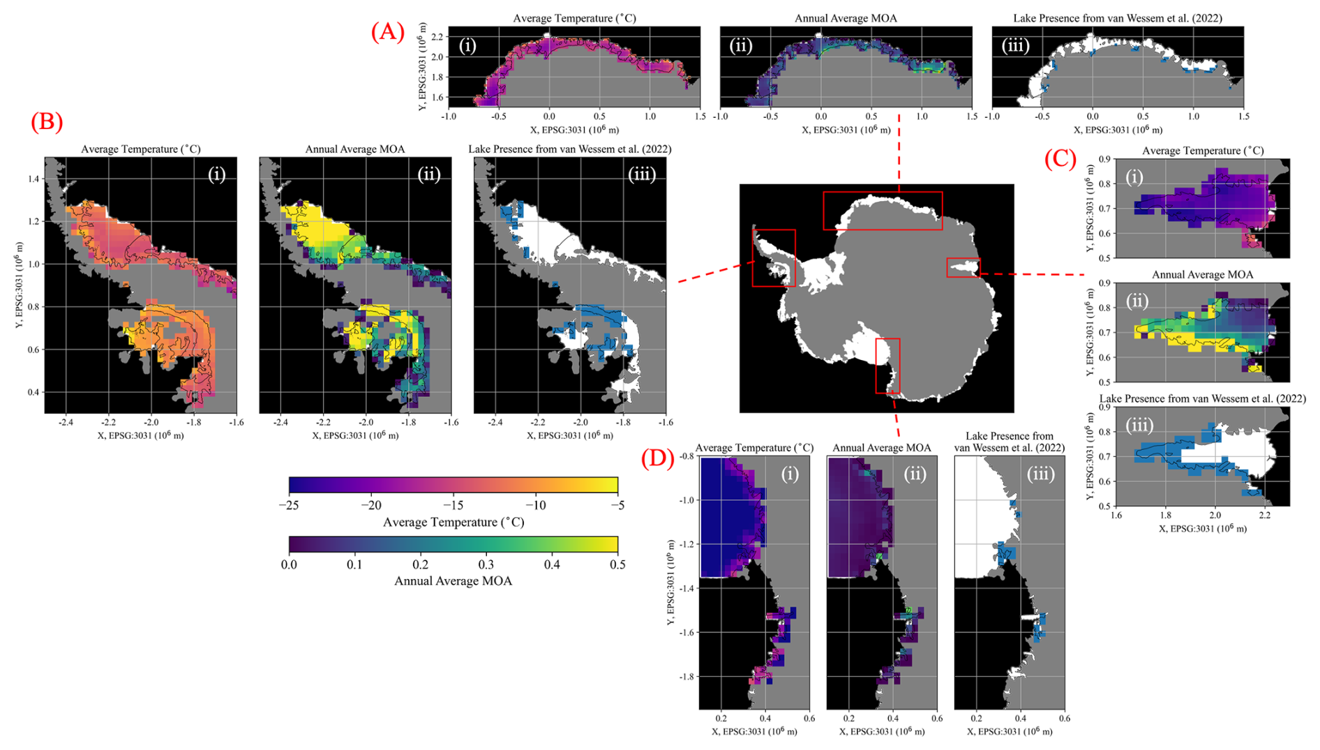
Figure 1 Regional climate data and binarized surface meltwater distribution across selected Antarctic ice-shelf areas at 27 km resolution. The central map shows all ice shelves with the four focus areas outlined: (a) Dronning Maud Land, (b) Antarctic Peninsula, (c) Amery Ice Shelf, and (d) western Ross Ice Shelf. For each region, panels (i)–(iii) show (i) average 2 m air temperature, (ii) annual average meltwater-over-accumulation (MOA), and (iii) observed surface meltwater distribution from van Wessem et al. (2022). Temperature and MOA are outputs from RACMO2.3p2 averaged over the period 1979–2022. Surface meltwater distribution is derived from Sentinel-2 imagery spanning austral summers 2015–2022 (van Wessem et al., 2022).

MOA thresholds have been used to predict future locations of surface ponding (e.g., van Wessem et al., 2023; Veldhuijsen et al., 2024), and are being implemented in the modeling protocol for the upcoming Ice Sheet Model Intercomparison Project for CMIP7 (Trusel et al., 2024). However, the performance of MOA as a predictive metric for ponding Antarctic-wide has never been directly quantified against present-day surface meltwater distributions. Van Wessem et al. (2023) noted that Antarctic-wide observations of surface meltwater broadly align with the MOA = 0.7 ponding threshold at a 27 km resolution, but this used only a qualitative comparison. In this work, we evaluate the performance of MOA as a predictive metric for surface ponding on all Antarctic ice shelves at a variety of resolutions, using melt and accumulation data from a regional climate model and present-day surface meltwater presence derived from threshold- and machine learning-based models. We also examine ways to incorporate and assess additional features to help predict ponding by considering proximity to ice-shelf grounding lines (e.g. Kingslake et al., 2017).

2 Methods

2.1 Datasets

This study integrates various data sources to examine the factors controlling continent-wide ice-shelf surface hydrology. These include outputs from the Regional Atmospheric Climate Model (RACMO) at 27, 11, and 2 km resolutions, and three multi-year surface hydrology datasets. Average air temperature and annual average MOA were calculated over the full RACMO time span, from 1979 to 2022 or 2023, depending on the model iteration (see Table 1, Fig. 1i and ii, Fig. 2a–c, Appendix Fig. A1). Of the three surface hydrology datasets, two were derived from a pixel thresholding-based method developed by Moussavi et al. (2020) (Tuckett, 2025; van Wessem et al., 2022). The other dataset, from Dell et al. (2024a), was derived from a machine learning-based method. Each of these meltwater datasets was aggregated to match the 27 km RACMO2.3p2 grid, and the Tuckett (2025) dataset was also aggregated to the 11 km RACMO2.4p2 grid and 2 km statistically downscaled RACMO2.3p2 grid. See Appendix B for more information on RACMO versions (B1) and meltwater datasets (B2).

We evaluated different predictive metrics of ponding for our five aggregated lakes datasets – Tuckett (2025) at 2, 11, and 27 km resolutions, van Wessem et al. (2022) at 27 km resolution, and Dell et al. (2024a) at 27 km resolution. We henceforth refer to these comparison scenarios, i.e., combinations of each lakes dataset with a RACMO iteration, as Tuckett-2k, Tuckett-11k, Tuckett-27k, VW-27k, and Dell-27k (Table 1). We use the full temporal extents of both the RACMO climate variables and the lakes datasets to capture processes relevant to both seasonal surface ponding and prior firn preconditioning. Figure 3 summarizes products and comparison scenarios used in this study.

Table 1 Summary of different comparison scenarios.

Figure 2 MOA data and surface meltwater distribution across the Antarctic Peninsula at three resolutions. The top row shows annual average MOA from (a) downscaled RACMO2.3p2 (1979–2023; Noël et al., 2023a), (b) RACMO2.4p1 (1979–2023; van Dalum et al., 2025), and (c) RACMO2.3p2 (1979–2022; van Wessem et al., 2022). The bottom row shows surface meltwater distribution derived from Landsat 7 and 8 imagery (Tuckett, 2025), aggregated to match the grids of the three RACMO outputs at (d) 2, (e) 11, and (f) 27 km resolutions.

2.2 Binarization of surface meltwater products

We converted our aggregated lakes datasets into binary products by defining lake coverage thresholds at which we would consider each grid cell a “lake” location. For the three Tuckett data products and the Dell-27k product, we used normalized lake presence thresholds, based on the number of times each ice-shelf pixel within a grid cell was identified as a lake (Fig. 2d–f, see Appendix B2 for details). For VW-27k, we used a threshold of 20 mm of aggregate meltwater depth, following the process of van Wessem et al. (2023) (Fig. 1iii). Lakes datasets and RACMO outputs were clipped to ice-shelf extents using shapefiles from MEaSUREs v.2 (Mouginot et al., 2017) and Dell et al. (2024a). Note that these shapefiles postdate the collapses of Larsen A and B ice shelves, and so these are not included in our analysis.

With our chosen thresholds, 4.6 % of ice-shelf grid cells in Tuckett-27k, 8.5 % in VW-27k, and 9.6 % in Dell-27k are classified as lake locations (Fig. 4). While our thresholds are necessarily subjective, they effectively highlight systematic differences in spatial distributions of meltwater between the three products. Tuckett-27k and VW-27k show broadly similar patterns, likely because both are derived from the same detection algorithm, though VW-27k identifies a greater number of meltwater grid cells overall. Dell-27k contains fewer grid cells above its meltwater threshold than Tuckett-27k or VW-27k on the Antarctic Peninsula, particularly along the coast of the Larsen C Ice Shelf, but more on the western Ross Ice Shelf.

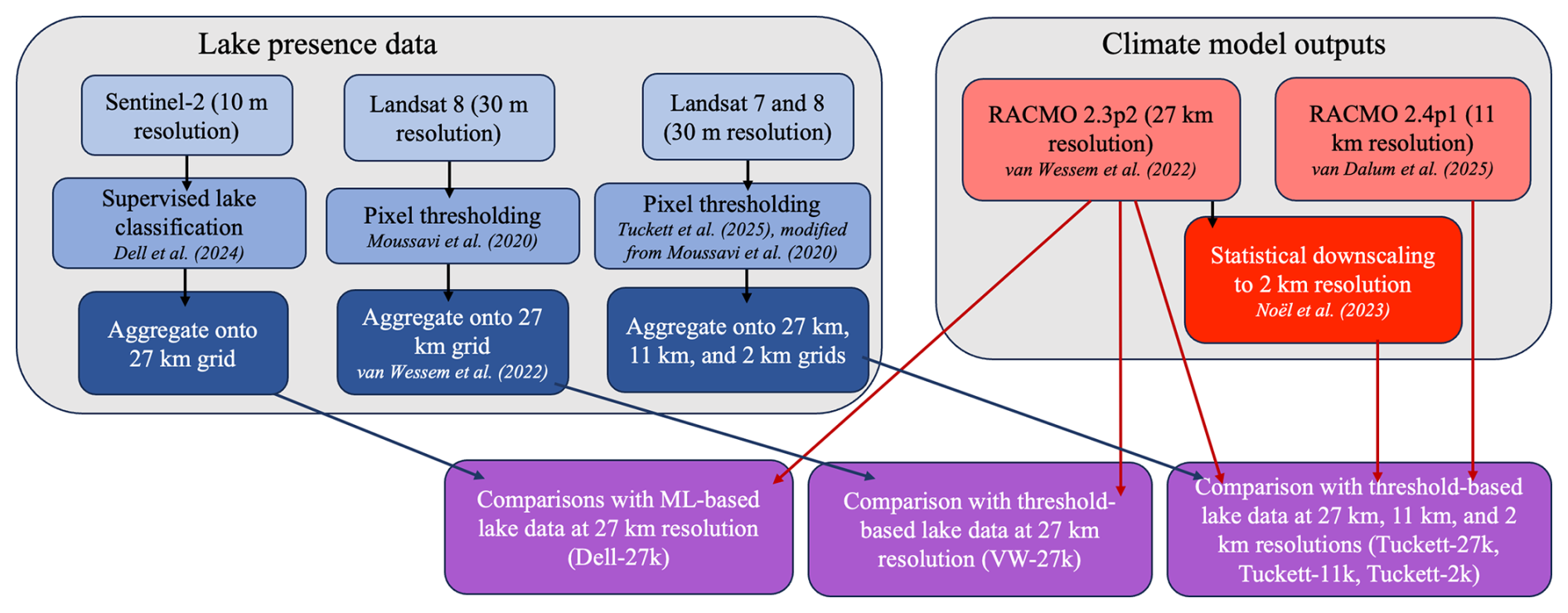
Figure 3 Overview of datasets and workflows used to compare lake presence data with regional climate model outputs. The blue boxes (left) represent three lake presence datasets derived from Sentinel-2 and Landsat imagery using supervised classification (Dell et al., 2024a) and pixel thresholding (Moussavi et al., 2020; Tuckett et al., 2025), aggregated to coarser spatial grids for comparison with climate model outputs. The red boxes (right) represent RACMO regional climate model outputs at 27 km (RACMO2.3p2; van Wessem et al., 2022) and 11 km (RACMO2.4p1; van Dalum et al., 2025) resolutions, as well as RACMO2.3p2 statistically downscaled to 2 km resolution (Noël et al., 2023a). The purple boxes (bottom) represent our five comparison scenarios resulting from different combinations of lake and climate data.

2.3 Calculation of Grounding Line Proximity Index (GLPI)

We defined a Grounding Line Proximity Index (GLPI) to investigate the predictive power of a spatially based proxy in addition to the climate model outputs. GLPI was calculated as the fraction of area within an 81 km radius of a grid-cell center that is composed of grounded ice. More explanation of the GLPI variable, including the choice of an 81 km radius, is provided in Results Sect. 3.3. We calculated a GLPI for every RACMO grid cell at 27, 11, and 2 km resolution, using grounding line positions from the MEaSUREs v.2 Antarctic Boundaries dataset (Mouginot et al., 2017).

2.4 Evaluating predictive performance

For each comparison scenario, we quantified the robustness of predictive metrics of ponding, including average near-surface temperature and annual average MOA. We systematically varied temperature threshold values between −30 and 0 °C with increments of 0.1 °C, and MOA threshold values between 0 and 1.5 with increments of 0.01. A MOA greater than 1 implies that annual snow- and firn- pack melt exceeds fresh snow accumulation, meaning that previous years' firn layers are being melted as well. We also evaluated the performance of a weighted sum threshold of MOA and GLPI, as follows:

$$\begin{array}{}\text{(3)}& {\mathrm{sum}}_{\mathrm{th}}=\mathrm{MOA}+c\left(\mathrm{GLPI}\right).\end{array}$$

We systematically varied both c, the weight coefficient on GLPI, and sum_th, the weighted sum. A grid search was performed over all combinations of c and sum_th, with values ranging from 0 and 10 with increments of 0.01 for both variables.

For each of the three types of criterion, we calculated the recall and precision of lake detection for each threshold, as follows:

$$\begin{array}{}\text{(4)}& \mathrm{recall}={\displaystyle \frac{\mathrm{TP}}{\mathrm{TP}+\mathrm{FN}}},\mathrm{precision}={\displaystyle \frac{\mathrm{TP}}{\mathrm{TP}+\mathrm{FP}}}.\end{array}$$

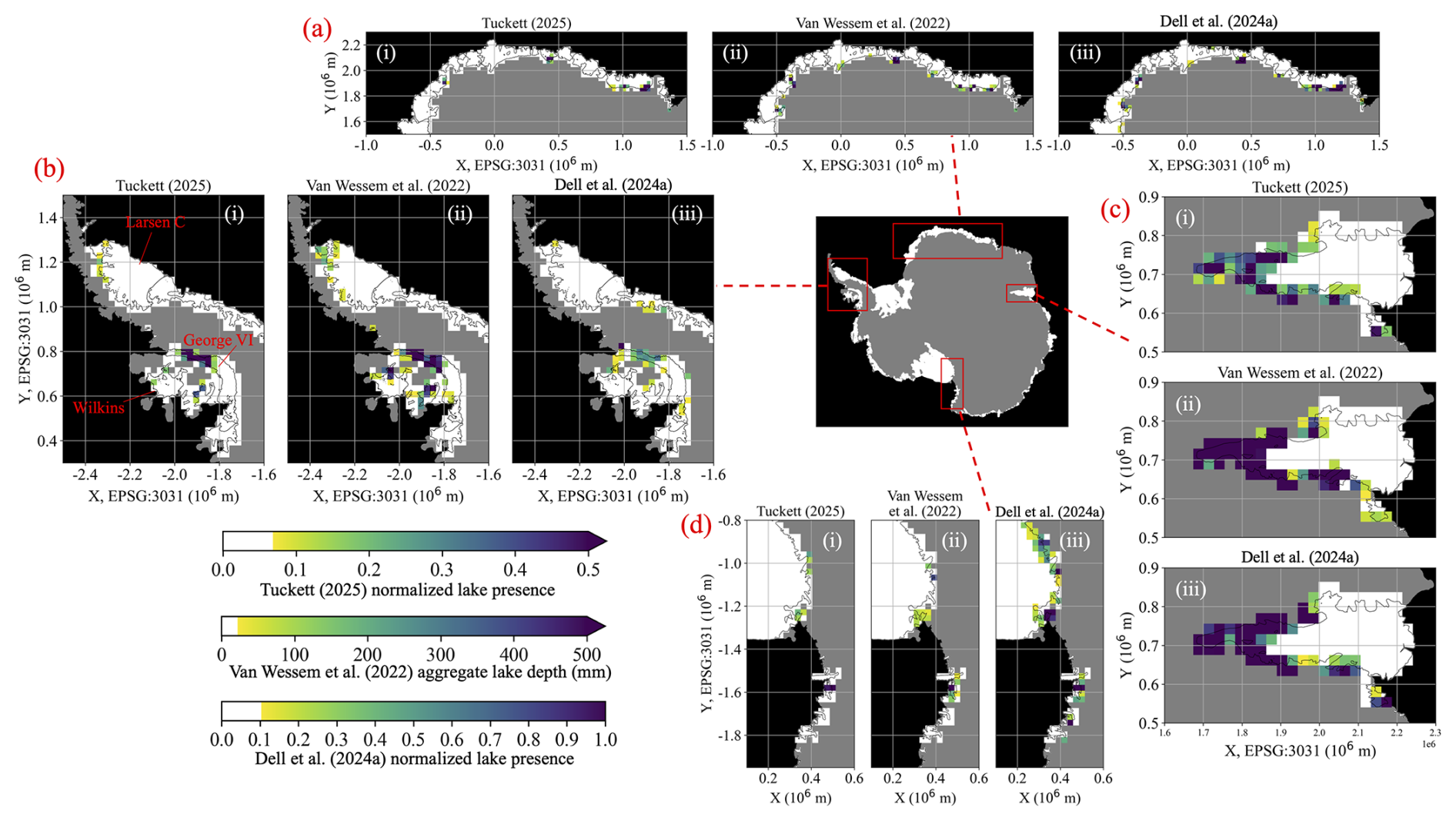
Figure 4 Surface meltwater distribution across selected Antarctic ice-shelf areas at 27 km resolution. The central map shows all ice shelves with the four focus areas outlined: (a) Dronning Maud Land, (b) Antarctic Peninsula, (c) Amery Ice Shelf, and (d) western Ross Ice Shelf. For each region, panels (i)–(iii) show observed surface meltwater aggregated on to the 27 km RACMO2.3p2 grid as follows: (i) normalized lake presence from 2006–2021 (Tuckett, 2025) (ii) aggregate meltwater depth from austral summers 2015–2022 (van Wessem et al., 2022), and (iii) normalized lake presence from austral summers 2013–2021 (Dell et al., 2024a). White areas indicate insufficient meltwater to reach the binarizing threshold for each data set (see text for more details). Locations of Antarctic Peninsula ice shelves mentioned in the text are indicated in panel (bi).

Recall represents the percentage of grid cells correctly identified by a given criterion as having surface meltwater (true positives, TP), out of all grid cells where the optical data actually detected surface meltwater (TP and false negatives, FN). Precision represents the percentage of grid cells correctly identified as having surface meltwater (TP) out of all grid cells that the threshold predicted as having surface meltwater (TP and false positives, FP). The F1 score was calculated for each threshold as the harmonic mean of precision and recall:

$$\begin{array}{}\text{(5)}& \mathrm{F}\mathrm{1}={\displaystyle \frac{\mathrm{2}}{{\mathrm{recall}}^{-\mathrm{1}}+{\mathrm{precision}}^{-\mathrm{1}}}}.\end{array}$$

We identified the optimal threshold for each criterion type for each comparison scenario as the one that maximized the F1 score. Appendix Fig. A2 shows how recall and precision vary with temperature and MOA thresholds for all five comparison scenarios.

After identifying the ponding threshold that corresponds with the highest F1 score, we applied this optimal threshold to RACMO2.3p2 modeled climate projections out to 2100 at 27 km resolution. We compared the resulting predicted lake coverage with that predicted using the literature standard of MOA ≥ 0.7.

3 Results

In this section, we quantify the performance of temperature, MOA, and MOA combined with GLPI as metrics for predicting the present day distribution of surface meltwater on Antarctic ice shelves, as delineated in each of our five comparison scenarios (Fig. 3). Appendix Fig. A3 summarizes the performance of all three metric types across these five scenarios continent-wide. We then discuss what these predictors imply for future meltwater ponding projections out to 2100.

3.1 Average air temperature

Figure 5a shows how F1 scores vary with temperature thresholds for all five comparison scenarios, for the entire ice sheet, the Antarctic Peninsula, and the ice sheet excluding the Peninsula. The peaks in F1 score indicate the optimal temperature thresholds for each region and scenario; lower temperature thresholds produce many false positives, while higher thresholds produce many false negatives. The F1 peak therefore represents the optimal balance. Where the curves flatten, at the low end of the temperature range for the Peninsula and the high end for the rest of the ice sheet, we can assume there are no grid cells within those temperature ranges, so changing the threshold does not influence predictive performance.

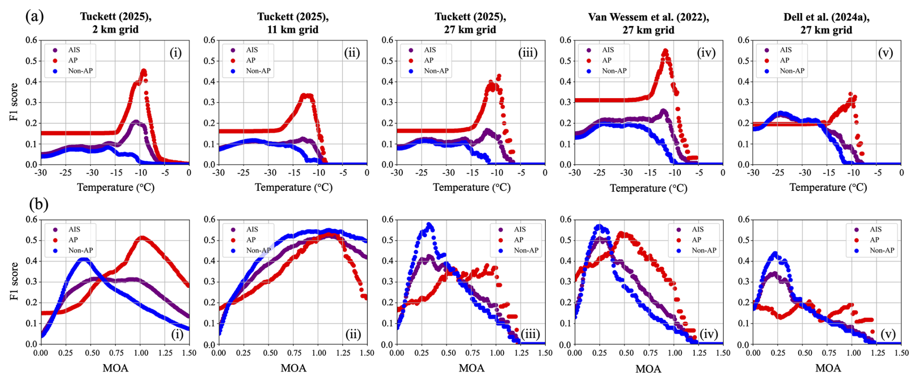
Figure 5 Performance of temperature and MOA thresholds as predictors of surface meltwater distribution across all five comparison scenarios. Each panel shows F1 scores as a function of (a) average temperature or (b) annual average MOA for the entire Antarctic Ice Sheet (AIS; purple), the Antarctic Peninsula (AP; red), and the remainder of the ice sheet excluding the Peninsula (Non-AP; blue). Results are shown for lakes datasets from Tuckett et al. (2025) at 2, 11, and 27 km resolutions (i, ii, iii), van Wessem et al. (2022) at 27 km resolution (iv), and Dell et al. (2024a) at 27 km resolution (v). Temperatures and annual MOA's are averaged over the period 1979–2022 or 2023, as indicated in Table 1.

Table 2 summarizes the performance of average air temperature as a predictor of present-day surface meltwater distribution. It includes the optimal temperature threshold, corresponding F1 score, and F1 score at the threshold found in literature (−9 °C; Cook and Vaughan, 2010; Morris and Vaughan, 2003) for each scenario and region.

Table 2 F1 scores for melt pond distribution prediction based on average air temperature thresholds. The bolded values indicate the two highest temperature threshold F1 scores for each region.

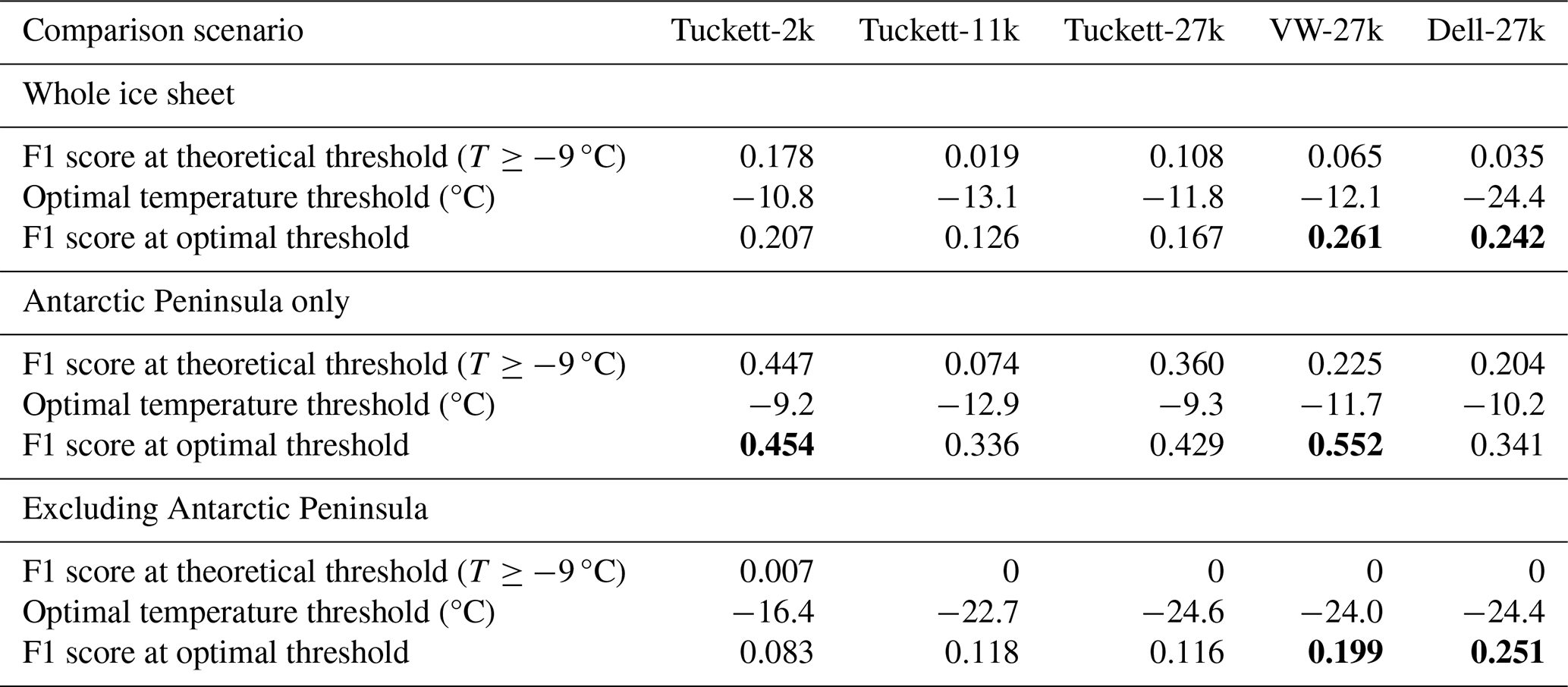
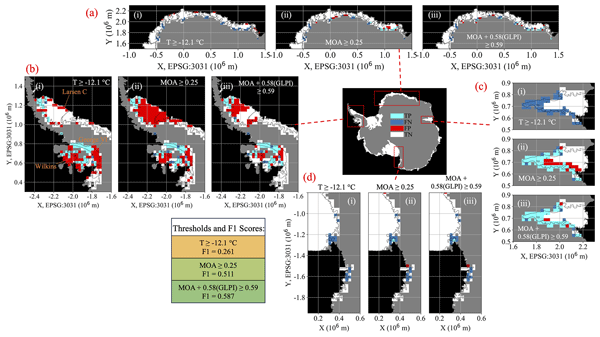
A mean annual isotherm of −9 °C has been proposed as a critical limit for ice-shelf stability, based on observations of surface-meltwater-induced ice-shelf collapse on the Antarctic Peninsula (Cook and Vaughan, 2010; Morris and Vaughan, 2003). However, using $T\ge -\mathrm{9}$ °C as a ponding threshold vastly underpredicts present-day lakes, resulting in F1 scores less than 0.2 for all five comparison scenarios where the whole ice sheet was being considered. The optimal predictive temperature was found to be lower: around −11 to −13 °C for VW-27k and the three Tuckett cases, and −24.4 °C for Dell-27k. Even at these optimal temperature thresholds, however, the highest F1 score for the entire continent, from VW-27k, is just 0.261. These results indicate that no single temperature threshold is an effective predictor of melt pond distribution continent-wide. A uniform temperature threshold overpredicts lakes on the Antarctic Peninsula (i.e., false positives), particularly on George VI and Wilkins Ice Shelves, and underpredicts elsewhere (i.e., false negatives), particularly on the Amery Ice Shelf and western Ross Ice Shelf (see i panels of Fig. 6). This broadly corroborates the findings of van Wessem et al. (2023), who noted that variable temperature thresholds for ponding are correlated with the amount of snowfall in a given region.

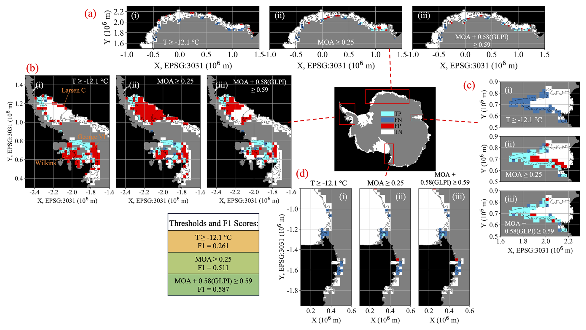
Figure 6 True positive, false negative, false positive (TP/FN/FP) masks for the VW-27k comparison scenario across selected Antarctic ice-shelf areas. Results are shown for the optimal continent wide thresholds based on (i) temperature, (ii) MOA, or (iii) combined MOA and GLPI. The central map shows all ice shelves with the four focus areas outlined: (a) Dronning Maud Land, (b) Antarctic Peninsula, (c) Amery Ice Shelf, and (d) western Ross Ice Shelf. For each region and threshold type, 27 km ice-shelf grid cells are colored to indicate true positives (light blue; correctly identified lake grid cells), false negatives (dark blue; observed lake grid cells not captured by the threshold), false positives (red; dry grid cells incorrectly classified as lakes), or true negatives (white; correctly identified dry grid cells). Locations of Antarctic Peninsula ice shelves mentioned in the text are indicated in panel (bi). The red-green color scale of the threshold text boxes represents the value of the F1 scores, and is consistent amongst Figs. 6, 7, and A3.

Temperature proved to be a more effective predictor when confining the study to the Antarctic Peninsula alone. In particular, in the VW-27k case, a threshold of $T\ge -\mathrm{11.7}$ °C on the  Peninsula corresponds with an F1 score of 0.552 (Fig. 7aiv). Tuckett-2k and Tuckett-27k perform almost as well (F1 scores of 0.454 and 0.429, respectively) at their optimal temperatures on the Peninsula, while Tuckett-11k and Dell-27k yield F1 scores of around 0.34. All five cases have higher optimal temperature thresholds on the Peninsula than on the rest of the continent (Fig. 5a). This corroborates the findings of van Wessem et al. (2023), who noted that ice shelves with more snowfall, such as those on the Peninsula, can withstand higher temperatures before forming surface ponds compared with the colder ice shelves in East and West Antarctica that receive less snowfall.

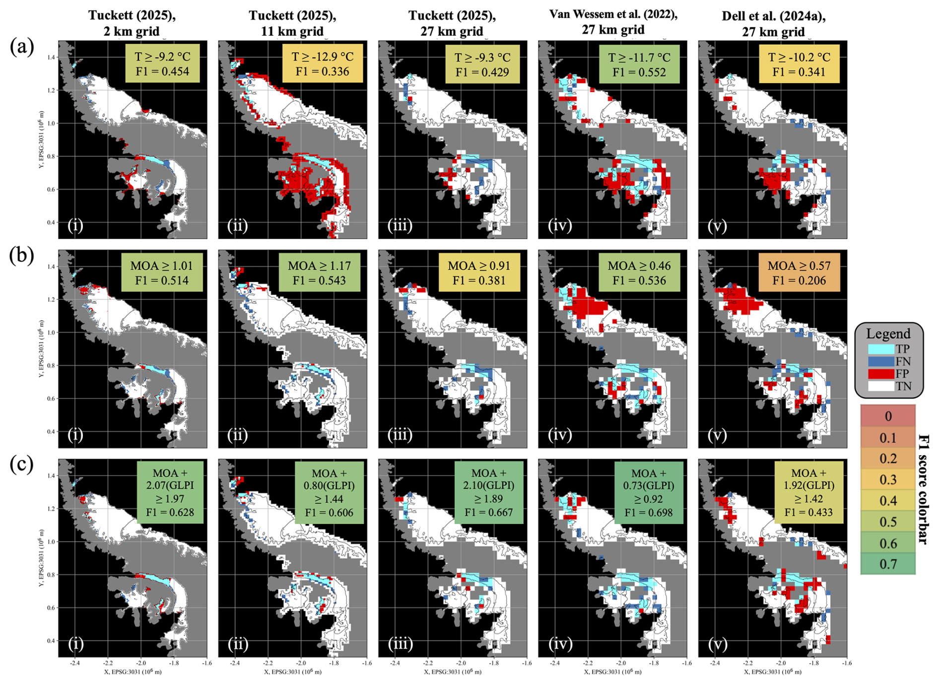
Figure 7 True positive, false negative, false positive (TP/FN/FP) masks for all comparison scenarios across Antarctic Peninsula ice shelves. Results are shown for the optimal Peninsula-only thresholds based on (a) temperature, (b) MOA, or (c) combined MOA and GLPI for comparison scenarios (i) Tuckett-2k, (ii) Tuckett-11k, (iii) Tuckett-27k, (iv) VW-27k, and (v) Dell-27k. For each scenario and threshold type, ice-shelf grid cells are colored to indicate true positives (light blue; correctly identified lake grid cells), false negatives (dark blue; observed lake grid cells not captured by the threshold), false positives (red; dry grid cells incorrectly classified as lakes), or true negatives (white; correctly identified dry grid cells). The red-green color scale of the overlying text boxes represents the value of the F1 scores, and is consistent amongst Figs. 6, 7, and A3.

3.2 Annual average MOA

Figure 5b presents how F1 scores vary with mean annual MOA thresholds for each comparison scenario and region. Similar to the temperature relationships, the peak of each curve marks the optimal MOA threshold that best predicts observed lake presence, balancing false positives and false negatives. With the exception of some of the Peninsula-only tests, we see that MOA is a more accurate predictor of surface ponding than temperature alone, yielding higher F1 scores at the optimal thresholds. Table 3 summarizes the performance of annual average MOA as a predictor of present-day surface meltwater distribution.

Table 3 F1 scores for melt pond distribution prediction based on annual average MOA thresholds. The bolded values indicate the two highest MOA threshold F1 scores for each region.

The theoretical MOA threshold of 0.7 is considerably too high for all three continent-wide 27 km comparison scenarios; the optimal MOA thresholds for these are all ∼ 0.2–0.3, whereas a threshold of 0.7 yields F1 scores below 0.3, much lower than the F1 peaks (Fig. 5biii–v). The optimal threshold is closest to 0.7 in Tuckett-2k (MOA ≥ 0.59), but only corresponds with an F1 score of 0.317 (Fig. 5bi). The optimal threshold is higher than 0.7 only in Tuckett-11k (MOA ≥ 1.11), but this scenario does not exhibit a distinct F1 score peak, i.e., there is no single MOA value that clearly maximizes predictive performance (Fig. 5bii).

Aside from Tuckett-11k, the VW-27k scenario yielded the best predictions from both temperature and MOA. In this scenario, a MOA of 0.25 corresponds with an F1 score of 0.511, nearly double that of the optimal temperature threshold (0.261). However, even this optimized threshold misses nearly all the lakes near the grounding line in the western Ross Ice Shelf (Fig. 6dii) and many in Dronning Maud Land (Fig. 6aii), while overpredicting lakes on the Amery Ice Shelf (Fig. 6cii) and the Antarctic Peninsula (Fig. 6bii), particularly at sites far from grounding lines.

Furthermore, and similar to temperature, the optimal MOA threshold varies regionally. In all five scenarios, when excluding the Antarctic Peninsula, the optimal threshold either barely changes or stays the same, but with improved F1 score performance. Looking at just the Peninsula, however, the optimal threshold increases to values of ∼ 1 in the Tuckett cases, and ∼ 0.5–0.6 for VW-27k and Dell-27k (Fig. 7b), values that would miss most of the lakes elsewhere in Antarctica. This regional variability in the MOA threshold could be attributed to limitations in the coarse resolution climate models, discussed in the following section.

3.3 Weighted sum of MOA and GLPI

While regional climate models such as RACMO effectively capture large-scale climate patterns (Kittel et al., 2021; Mottram et al., 2021; van Dalum et al., 2025; van Wessem et al., 2018; Wang et al., 2025), their coarse grids cannot resolve local processes that can strongly influence ice-shelf surface mass balance, including orographic precipitation, small-scale albedo variations, and foehn winds (Datta et al., 2018; de Roda Husman et al., 2024; Kingslake et al., 2017; Noël et al., 2023a). The 2 km resolution RACMO dataset addresses these limitations through statistical downscaling based on local albedo and surface topography (Noël et al., 2023a).

Here, we adopt a crude proxy to approximate these effects at each resolution: using proximity to the grounding line as an indicator of processes that enhance melt. Ice near the grounding line is more likely to contain exposed rocky outcrops or blue ice, both of which lower the local albedo (Kingslake et al., 2017). Furthermore, steeper surface slopes near the grounding zone increase the warming effects of atmospheric dynamics such as foehn winds (Datta et al., 2018, 2019; Laffin et al., 2022). These effects are not incorporated into RACMO, so may explain why a uniform MOA threshold misses lakes in regions close to the grounding line (i.e., in Dronning Maud Land and western Ross Ice Shelf, see Fig. 6a, dii). Similarly, this threshold overpredicts lakes in regions with higher MOA far from the grounding line (e.g., on Larsen C and Amery ice shelves, see Fig. 6b–cii).

To represent these influences, as mentioned in Methods Sect. 2.3, we assigned each RACMO grid cell a Grounding Line Proximity Index (GLPI), defined as the percentage of grounded pixels within an 81 km radius of the grid cell center. The 81 km radius was chosen to balance the local influence of albedo with the broader reach of foehn winds, which have been shown to enhance surface melt as far as 100 km from the foot of the mountains on the Antarctic Peninsula (Turton et al., 2020). This radius therefore captures the dominant length scales of both processes, while also aligning neatly with the width of three RACMO2.3p2 grid cells.

We tested the predictive power of GLPI combined with MOA by taking a weighted sum of the two metrics at each grid cell, as defined in Eq. (3). Table 4 shows the optimal GLPI weights (c) and weighted sum thresholds (sum_th) for each of the five comparison scenarios, along with the corresponding F1 scores.

Incorporating GLPI improves the predictive performance of MOA alone in all five comparison scenarios. As with both temperature and MOA, the weighted sum metric performs best in the VW-27k scenario, with a continent-wide F1 score of 0.587 using the threshold MOA + 0.58(GLPI) ≥ 0.59. This combined metric substantially decreases false positives far from the grounding lines on Larsen C, George VI, and Wilkins ice shelves on the Antarctic Peninsula, as well as on Amery Ice Shelf (Fig. 6b–ciii), yet still misses most lakes on the western Ross Ice Shelf and shows only slight improvement in Dronning Maud Land (Fig. 6a, diii).

Table 4 F1 scores for melt pond distribution prediction based on weighted sums of annual average MOA and GLPI thresholds. The bolded values indicate the two highest MOA and GLPI threshold F1 scores for each region.

Even with GLPI, there is still an apparent regional difference in thresholds. Across all five scenarios, the optimal thresholds for both the weighted sum and the weight on GLPI (c) are higher for the Antarctic Peninsula (Fig. 7c) and lower for the rest of the ice sheet, relative to the whole continent. Isolating the Peninsula substantially improves the F1 score in all scenarios, particularly Tuckett-2k, Tuckett-27k, and VW-27k, while excluding the Peninsula slightly improves the F1 score, especially for Tuckett-27k and Dell-27k. The weighted sum threshold MOA + 0.73(GLPI) ≥ 0.92 for the Peninsula alone in the VW-27k scenario yields the highest F1 score in this study (0.698, see Fig. 7civ).

3.4 Future projections

The value of defining ponding thresholds from present-day surface melt distributions lies in their potential to predict future surface melt distributions. We used RACMO2.3p2 projections of average MOA from 2015 to 2100 to predict future lake locations under three emissions pathways: SSP1-2.6 (low emissions, ∼ 1.8 °C warming by 2100), SSP2-4.5 (intermediate emissions, ∼ 2.0 °C warming), and SSP5-8.5 (very high emissions, ∼ 2.4 °C warming) (IPCC, 2021). While snowfall is expected to increase quasi-linearly with temperature, melt production increases more than linearly (Donat-Magnin et al., 2021; Palerme et al., 2017; Trusel et al., 2015; van Wessem et al., 2023), leading to increases in MOA continent-wide across all pathways.

We compared two ponding thresholds: the “theoretical threshold”, i.e., the current literature standard, MOA ≥ 0.7 (Donat-Magnin et al., 2021; Pfeffer et al., 1991; van Wessem et al., 2023; Veldhuijsen et al., 2024), and the “empirical threshold”, i.e., the optimal continent-wide threshold from the VW-27k analysis, MOA + 0.58(GLPI) ≥ 0.59. In present-day conditions, these thresholds correspond with F1 scores of 0.261 (theoretical) and 0.587 (empirical) in the VW-27k scenario.

Using projected MOA values, we calculated the number of 27 km ice-shelf lake grid cells predicted under the theoretical and empirical thresholds under all three emissions pathways. Table 5 summarizes these results for the year 2100 based on the annual average MOA from 2090–2099, and Fig. 8 shows the temporal evolution of predicted lakes based on a ten-year rolling MOA average.

Table 5 Ten-year average MOA and predicted numbers of lake grid cells over Antarctic ice shelves in present day and in 2100 for three emissions pathways and two thresholds.

The theoretical threshold predicts only 56 lake grid cells under present-day conditions, whereas the empirical threshold predicts 255 grid cells, which is much closer to the observed value of 336 lake grid cells from the VW-27k dataset. The present-day data therefore suggest that the theoretical MOA threshold for ponding is too high. Because the empirical threshold better reproduces present-day lake extent, we expect it to provide more reliable projections of future conditions.

By 2100, the average MOA over Antarctic ice shelves is projected to increase from 0.106 to 0.294 under SSP1-2.6 (i panel of Fig. 9). Under these conditions, the empirical threshold predicts 732 lake grid cells, a 2.2 times increase in total ponding extent relative to today (iii panel of Fig. 9). Under SSP5-8.5, the average MOA is projected to increase almost tenfold, to 0.984. In this scenario, the empirical threshold predicts 2,399 lake grid cells in 2100, more than seven times the present-day extent (see Appendix Fig. A4). However, even these projected increases in lake coverage may be conservative. We cannot necessarily expect the relationship between MOA and ponding to remain static over time, as processes that precondition the firn for ponding, such as ice lens formation, are expected to increase as the climate warms (Veldhuijsen et al., 2024) (see Discussion Sect. 4.4 for more details).

The uncertainty arising from threshold choice is comparable in magnitude to uncertainty due to emissions pathways (Fig. 8). Using the theoretical threshold, the projected difference in lake presence in 2100 between the highest and lowest emissions scenarios (SSP5-8.5 and SSP1-2.6) is 1397 grid cells. By comparison, under SSP5-8.5 alone, the difference between predictions using empirical and theoretical thresholds is 685 grid cells. Between the two lower emissions pathways (SSP1-2.6 and SSP2-4.5), projected lake presence remains similar until around 2070, but there is a consistent difference of ∼ 300 lake grid cells between the theoretical and empirical threshold predictions.

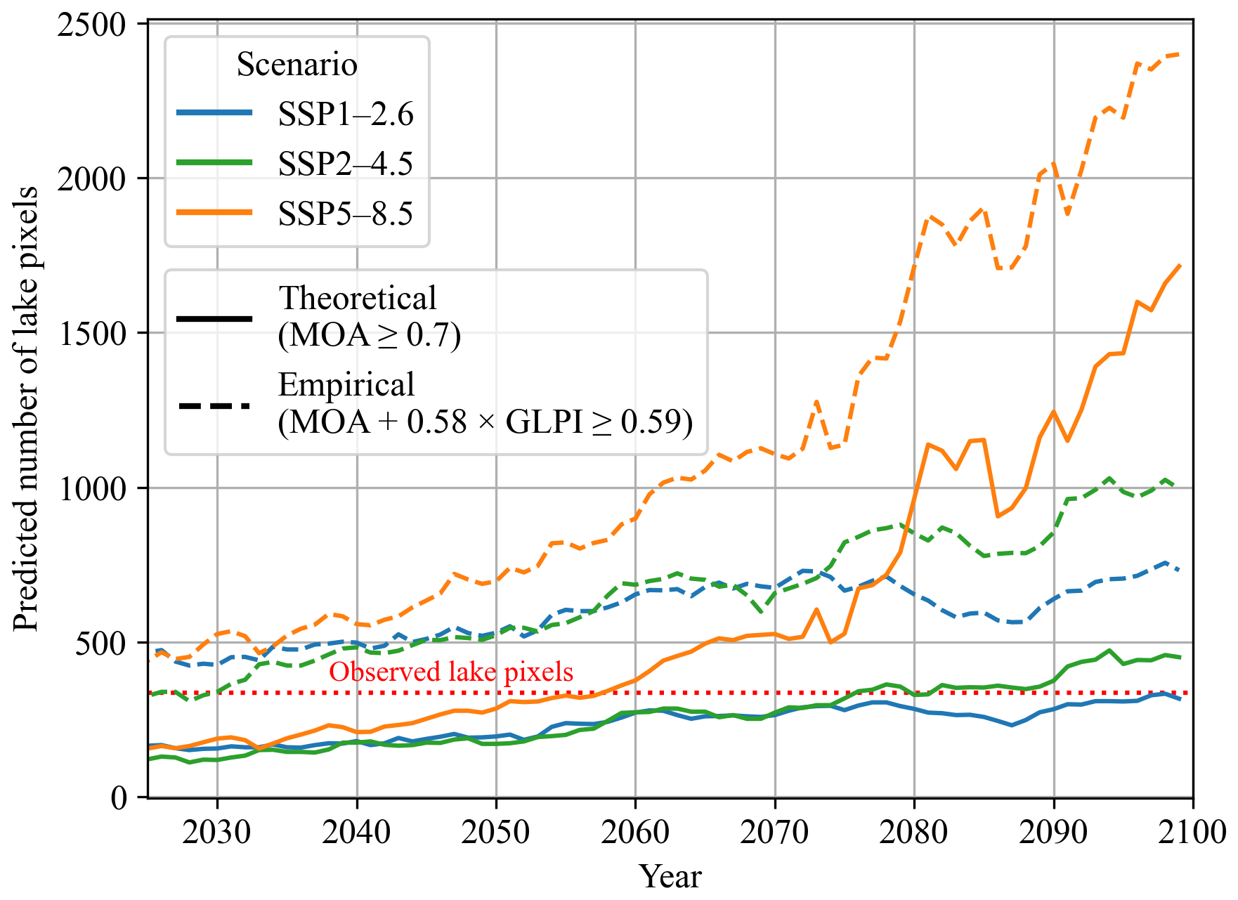
Figure 8 Projected number of 27 km lake grid cells across all Antarctic ice shelves from 2025–2100 under three emissions pathways. The solid lines represent projected lake presence based on the theoretical threshold of MOA ≥ 0.7, and the dashed lines represent projected lake presence based on the empirical continent-wide threshold of MOA + 0.58(GLPI) ≥ 0.59. The red dashed line represents the observed number of present-day lake grid cells (336) in the VW-27k lakes data product. MOA projections are ten-year rolling averages derived from RACMO2.3p2 climate model outputs (van Wessem et al., 2022).

All four areas of interest (Dronning Maud Land, Antarctic Peninsula, Amery Ice Shelf, and western Ross Ice Shelf) are projected to experience increased meltwater by 2100 under SSP1-2.6 with either threshold, but the empirical threshold predicts larger magnitudes of meltwater extent across all four areas (see Fig. 9). The fact that threshold choice introduces uncertainty comparable to that arising from emissions scenario selection underscores the importance of using empirically derived, observation-constrained thresholds when projecting future surface ponding.

Climate projections indicate that some ice-shelf regions, particularly the southwest corner of the Amery Ice Shelf, are expected to have negative MOA values in the future (Fig. 9ci). This occurs because projected annual sublimation eventually exceeds snowfall in magnitude, making the denominator of MOA in Eq. (1) negative. Our thresholds therefore do not predict lakes in this region (Fig. 9cii–iii). However, in reality, net removal of snow and firn would precondition the area for meltwater ponding. Appendix Fig. A4 shows that this underprediction of lakes on Amery persists amongst emissions pathways. Negative MOA values arise in 32, 45, and 18 grid cells in 2100 under SSP1-2.6, 2-4.5, and 5-8.5, respectively, causing a slight underestimation of total lake extent. To address this, Appendix C and Appendix Fig. C1 present a simple method to adjust MOA in high-sublimation and low-accumulation regions, which may become increasingly important under future climate scenarios.

Figure 9 Projections of MOA and lake distribution in 2100 under emissions pathway SSP1-2.6 across selected Antarctic ice-shelf areas at 27 km resolution. The central map shows all ice shelves with the four focus areas outlined: (a) Dronning Maud Land, (b) Antarctic Peninsula, (c) Amery Ice Shelf, and (d) western Ross Ice Shelf. For each region, panels (i)–(iii) show (i) projected annual average MOA from 2090–2099, (ii) projected surface meltwater distribution based on theoretical threshold of MOA ≥ 0.7, and (iii) projected surface meltwater distribution based on the empirical continent-wide threshold of MOA + 0.58(GLPI) ≥ 0.59. MOA projections are derived from RACMO2.3p2 climate model outputs (van Wessem et al., 2022). Location of the negative projected MOA values, in the southwest corner of Amery Ice Shelf, is indicated with orange arrows in panels (ci–iii).

4 Discussion

4.1 Comparison of lakes data products

In this work, we evaluated the effectiveness of temperature, MOA, and a weighted sum of MOA and GLPI as predictive metrics of ice-shelf surface ponding. At 27 km resolution, these metrics were assessed using three separate surface melt products: two generated from a pixel-identification algorithm (VW-27k and Tuckett-27k) and one from a machine learning-based method (Dell-27k). All three predictor types yielded the highest F1 scores when evaluated against VW-27k.

Tuckett-27k and VW-27k were derived from the same base lake identification algorithm, from Moussavi et al. (2020). This suggests that differences in how wet and dry grid cells are binarized, rather than the underlying detection approach, drive the observed performance differences. In particular, VW-27k identifies lake grid cells using aggregate water depth (van Wessem et al., 2023), whereas Tuckett-27k and Dell-27k rely on a normalized lake presence threshold based on binary heat maps. Weighting observations by total lake volume gives more confidence to deeper lakes, thus reducing the relative influence of potential false positives caused by spurious detections or blue ice. Weighting lake depth also helps account for water that may have drained from adjacent grid cells, suggesting a larger effective meltwater area. These results suggest that assessments of ice-shelf surface ponding conditions are most robust when based on lake-presence observations that explicitly incorporate lake depth.

The Dell et al. (2024) dataset was the only one to include slush in its assessment of wet areas. We also performed the Dell-27k analysis with the slush excluded, and found that this did not alter the conclusions.

4.2 Comparison of grid resolutions

We also examined how grid resolution influences the ability of MOA to predict surface ponding, using the Tuckett et al. (2025) product at 27, 11, and 2 km resolutions. MOA is best able to predict ponding at 11 km resolution (F1 = 0.523), followed by 27 km (F1 = 0.425) and 2 km (F1 = 0.317). Incorporating GLPI improves the F1 scores at all resolutions, but the ordering remains the same. The improved performance at 11 km likely reflects improvements in the underlying climate model; Tuckett-27k and Tuckett-2k were both compared with versions of RACMO2.3p2 (Noël et al., 2023a; van Wessem et al., 2018), whereas Tuckett-11k was compared with the newer RACMO2.4p1 (van Dalum et al., 2024a).

There are two notable differences in the performance of MOA between Tuckett-11k and the other resolutions. Firstly, as noted in Results Sect. 3.2, Tuckett-2k and Tuckett-27k exhibit distinct, narrow MOA peaks corresponding to optimal ponding prediction values (Fig. 5bi, iii). In contrast, Tuckett-11k shows a wider range of MOA values with comparably high predictive skill (Fig. 5bii). The generally higher MOA values generated from RACMO2.4p1 (van Dalum et al., 2025) reduce the occurrence of false negatives at higher thresholds, thus resulting in the broader range of effective MOA values. Secondly, the optimal MOA threshold over the Antarctic Peninsula in Tuckett-11k (1.17) is similar to that of the rest of the continent (1.11). For the other two resolutions, the threshold is much higher on the Peninsula (0.91 vs. 0.32 for Tuckett-27k, and 1.01 vs. 0.59 for Tuckett-2k). The updated atmospheric dynamics and blowing snow scheme in RACMO2.4p1 result in more precipitation and less sublimation over the Antarctic Peninsula (van Dalum et al., 2025), both of which lower the average MOA in that region (Fig. 2a–c). This brings the MOA values on the Peninsula closer to those in the rest of the continent, thus reducing the regional discrepancy in optimal thresholds.

However, the performance of MOA as a predictor depends not only on the underlying RACMO version, but also on the spatial resolution of analysis. Between the two resolutions of RACMO2.3p2, MOA performs substantially worse as a ponding predictor in the statistically downscaled case (Tuckett-2k). This result is noteworthy given that the downscaling to 2 km was shown to help the model better capture topographic controls on precipitation and to reduce the underestimation of melt near grounding lines that was present in the 27 km product (Noël et al., 2023a). These results suggest that MOA is inherently a more effective predictor of ponding at coarser spatial scales. While the downscaled model may better resolve local melt variability, MOA does not account for local processes such as meltwater transport and ice lenses. MOA is therefore a spatially integrated climate metric that is more closely aligned with regional melt regimes than meter-scale ponding processes. Consistent with this interpretation, MOA has predominantly been applied to predict ponding at regional to shelf- or glacier-wide scales (Pfeffer et al., 1991; van Wessem et al., 2023; Vries et al., 2025).

4.3 Influence of downslope winds

The statistical downscaling process of Noël et al. (2023a) incorporates albedo and surface topography into 2 km RACMO SMB estimates. However, while both of these factors enhance melt near grounding lines, incorporating grounding line proximity via GLPI still improves the predictive power of MOA in the downscaled comparison scenario. GLPI increases the F1 score in Tuckett-2k from 0.317 (MOA alone) to 0.425 (MOA with GLPI). This improvement indicates that GLPI captures additional grounding-line-adjacent melt processes. Notably, downslope winds, including katabatic and foehn flows, are a primary driver of surface melt near grounding lines (Laffin et al., 2023; Mahagaonkar et al., 2025), but are not represented in coarse-resolution climate models or in the RACMO downscaling process (Lenaerts et al., 2012; Noël et al., 2023a; Wiener et al., 2025).

Katabatic winds are density-driven winds that warm adiabatically as they flow downslope (Laffin et al., 2023; Lenaerts et al., 2017), and foehn winds arise when cool, moist air is forced over a mountain barrier (Datta et al., 2018, 2019). Both processes create warm near-surface air and scour the ice-shelf surface of loosely-packed, high-albedo snow and firn (Lenaerts et al., 2017; Trusel et al., 2013; Tuckett et al., 2021), thus optimizing the local environment for surface melting. These downslope winds have been estimated to contribute ∼ 20 % of surface melt on the Antarctic ice sheet over the last four decades (Laffin et al., 2023). This results in increased melt pond formation near the grounding zone of ice shelves, where downslope winds converge (Arthur et al., 2020; Kingslake et al., 2017; Tuckett et al., 2021). Foehn winds are especially prominent on the Antarctic Peninsula and in regions of East Antarctica. Foehn events have been shown to increase melt frequency on the northeastern Peninsula (Datta et al., 2018, 2019), to extend the length of the melt season on Larsen C (Turton et al., 2020), and to have contributed to melt pond formation preceding the collapses of the Larsen A and Larsen B ice shelves (Laffin et al., 2022). In Dronning Maud Land, both katabatic and foehn winds have been shown to increase the presence of lakes near grounding zones through snow erosion, scouring, and surface warming (Mahagaonkar et al., 2025). Similar influence of downslope winds on melt has been observed elsewhere in East Antarctica, including the Shackleton Ice Shelf (Saunderson et al., 2022) and the McMurdo Dry Valleys (Hofsteenge et al., 2022). The spatial influence of these winds on melt pond formation is implicitly captured by the GLPI. The prevalence of foehn winds on the Peninsula likely explains why in all five comparison scenarios, incorporating GLPI raises the F1 score much more for the Peninsula alone than for the rest of the continent. We also see that in Dronning Maud Land, the incorporation of GLPI removes some false negatives at the grounding line and some false positives further from the grounding line (Fig. 6aii, iii). However, the threshold still misses some lakes near the grounding line in the west side of the region. We emphasize that GLPI is not a physical mechanism, but rather a proxy for multiple processes that enhance surface melt, including downslope winds. GLPI does not account for the direction of these winds, and may overestimate melt on the upwind side of local topographic barriers. Future work could incorporate a directional component that would refine the index's physical accuracy. While statistical downscaling is a more rigorous method to incorporate these processes, GLPI is much less computationally complex, and its improvement to predictions highlights the need for incorporation of downslope winds.

4.4 Limitations of a MOA threshold

MOA thresholds account straightforwardly for firn air content, providing a more robust metric for predicting ice-shelf ponding distributions than temperature or SMB. However, the theoretical threshold of MOA ≥ 0.7 was determined based on assumptions about the initial firnpack, including a uniform temperature and density (Eq. 2) and the overly restrictive assumption that meltwater must completely saturate the firn air space before ponding initiation (Pfeffer et al., 1991). Furthermore, estimated values of melt and accumulation vary widely between climate models (Mottram et al., 2021; van den Broeke et al., 2023; Wirths et al., 2024). RACMO generally predicts higher Antarctic SMB values than other CMIP models (Mottram et al., 2021; Wang et al., 2025, 2016), such that a MOA threshold of 0.7 identifies just 16 % of lakes in the VW-27k comparison scenario (Appendix Fig. A2biv).

If MOA is to be used as a predictor of ponding, we recommend calibrating the threshold for the climate data being used, as done in this study. After calibration and incorporation of GLPI, MOA predicts continent-wide lake distribution with an F1 score of 0.587 in the VW-27k scenario. This represents a substantial improvement over the uncalibrated threshold (F1 = 0.261). However, a more accurate predictor would need to incorporate other climatic variables. We used multi-decadal average MOA values to represent the potential timescale of firn air depletion, but this long-term averaging deemphasizes warm temperature extremes and positive degree days, both of which have been tied to increased melting on the Antarctic Peninsula (Barrand et al., 2013; Trusel et al., 2015; Vaughan, 2006; Zheng et al., 2023). A simple temperature threshold performs comparably well to MOA as a ponding predictor on the Peninsula; for VW-27k, F1 = 0.552 for temperature and 0.536 for MOA, likely because temperatures in this region are warm enough to drive ponding regardless of firnpack preconditioning.

No single climate-based threshold has been identified as a universal predictor of ponding, due to inherent limitations in regional climate models. In addition to the downslope winds discussed in the previous section, melt-albedo feedbacks (Jakobs et al., 2021; Kingslake et al., 2017), drifting snow (Amory, 2020), and changing albedo due to grain growth (Arioli et al., 2023; Behn et al., 2021) are all examples of factors which can influence melt yet are not accounted for in most climate models (Tuckett et al., 2021; van den Broeke et al., 2023).

Another important process missing from climate models is the formation of ice lenses or slabs, caused by refreezing meltwater in the firnpack, which create impermeable layers that block meltwater percolation (Veldhuijsen et al., 2024). This process reduces the accessible firn air content and has been demonstrated to facilitate ponding initiation earlier than a simple MOA threshold would predict (Buzzard et al., 2018; Dunmire et al., 2024). A recent (2006–2021) increase in meltwater across the East Antarctic Ice Sheet, despite relatively consistent snowmelt rates, has been linked to ice lenses lowering permeability (Tuckett et al., 2025).

As the climate continues to warm, the differences between total and accessible firn air content due to ice lens formation are projected to increase (Veldhuijsen et al., 2024), underscoring the need to exercise caution when predicting meltwater based on MOA. Ice lens formation is difficult to predict; they tend to proliferate in “intermediate warm” and relatively low-precipitation regions, where melt is sufficient to form lenses but not to fully saturate the firn layer, and in areas with high interannual variability in melt (Veldhuijsen et al., 2024). This implies that the MOA threshold for ponding may decrease over time with complex spatial heterogeneity. Coupling a climate model to a firn model or emulator (e.g., Dunmire et al., 2024; Thompson-Munson et al., 2023), could increase the accuracy of ponding predictions. However, this process would be computationally expensive at a continent-wide scale.

Due to the multitude of processes contributing to surface pond formation, region-specific climate thresholds are likely necessary for accurate ponding predictions. The role of downslope winds in driving surface melt varies across regions, depending on local topography and prevailing atmospheric conditions. East Antarctica experiences a high proportion of wind-driven surface melt (Laffin et al., 2023), so likely corresponds with a higher dependence on GLPI or a similar index than West Antarctica. East Antarctic ice shelves contain more widespread ice lenses within the firn than other regions (Tuckett et al., 2025), and both East Antarctic and Antarctic Peninsula shelves are predicted to experience increased ice lens formation between now and 2100 (Veldhuijsen et al., 2024). This suggests lower future MOA thresholds in these regions. As ice lens formation intensifies under future warming, these regional differences in ponding susceptibility may become increasingly pronounced.

5 Conclusions

Accurately predicting the distribution of surface meltwater on Antarctic ice shelves is critical for assessing areas that could be vulnerable to hydrofracture, particularly in regions of high extensional stress (Lai et al., 2020). In this paper, we quantified the performance of average air temperature, annual average MOA, and a weighted sum of MOA and GLPI as predictors of surface ponding for three different lakes datasets and three climate model grid resolutions. We find that the predictive power of MOA depends strongly on both climate forcing and region, and that it can be improved by incorporating GLPI to account for grounding line-adjacent processes that exert an important control on pond formation.

Empirically calibrated thresholds consistently outperform the theoretical threshold of MOA ≥ 0.7. For the VW-27k comparison scenario under emissions pathway SSP1-2.6, applying the optimized continent-wide threshold (F1 = 0.587) predicts 2.3 times more lake coverage in 2100 than the theoretical threshold (F1 = 0.261). Across data products, future projections using empirically calibrated thresholds yield substantially greater surface ponding than projections based on the theoretical threshold, suggesting that reliance on MOA ≥ 0.7 may systematically underestimate future meltwater extent on Antarctic ice shelves. Optimal threshold values differ between the Antarctic Peninsula and the remainder of the ice sheet, reflecting regional differences in melt processes, firn conditions, and the influence of downslope winds. For the VW-27k scenario, we identify optimal thresholds of MOA + 0.73(GLPI) ≥ 0.92 for the Antarctic Peninsula (F1 = 0.698) and MOA + 0.34(GLPI) ≥ 0.42 for the rest of the continent (F1 = 0.626).

Although MOA relies on simplifying assumptions about firn properties and does not explicitly resolve processes such as ice lens formation, it remains a simple, physically interpretable, and computationally efficient framework for predicting meltwater presence. If MOA is to be used as a diagnostic tool, we recommend it be applied at relatively coarse spatial scales (tens of kilometers), and that the threshold value be calibrated to the specific climate forcing using depth-weighted present-day lake observations. We also suggest that MOA be augmented to account for grounding line-adjacent melt processes, including downslope winds. Used in this way, MOA provides a practical tool for identifying ice-shelf regions susceptible to surface ponding and potential collapse.

Appendix A: Additional figures

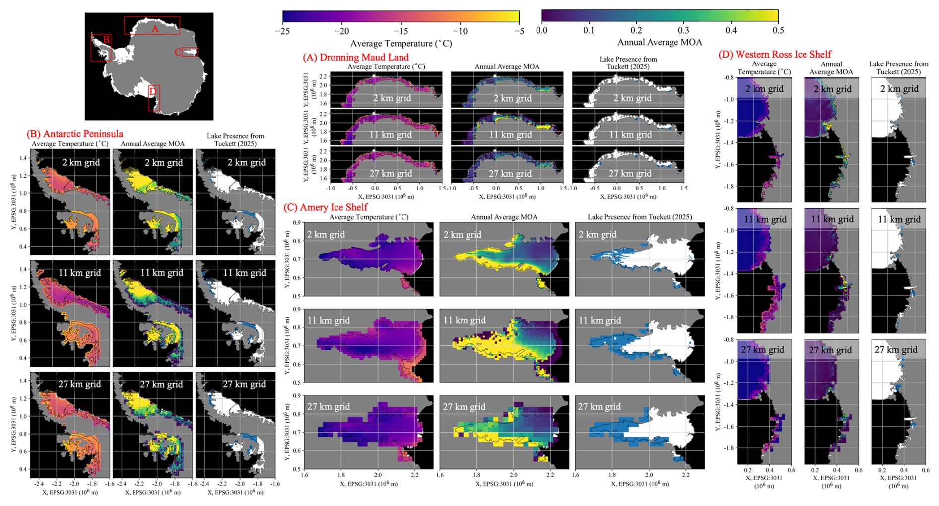
Figure A1 Regional climate data and binarized surface meltwater distribution across selected Antarctic ice-shelf areas at 2, 11, and 27 km resolutions. The map in the upper left shows all ice shelves with the four focus areas outlined: (a) Dronning Maud Land, (b) Antarctic Peninsula, (c) Amery Ice Shelf, and (d) western Ross Ice Shelf. For each region, panels show average 2 m air temperature (left columns), annual average meltwater-over-accumulation (MOA) (center columns), and observed surface meltwater distribution from Tuckett (2025) (right columns). Data is shown at 2 km resolution (top rows), 11 km resolution (center rows), and 27 km resolution (bottom rows). Surface meltwater distribution is derived from Landsat 7 and 8 imagery spanning 2006–2021 (Tuckett, 2025). RACMO climate model iterations and time spans for temperature and MOA outputs can be seen in Table 1.

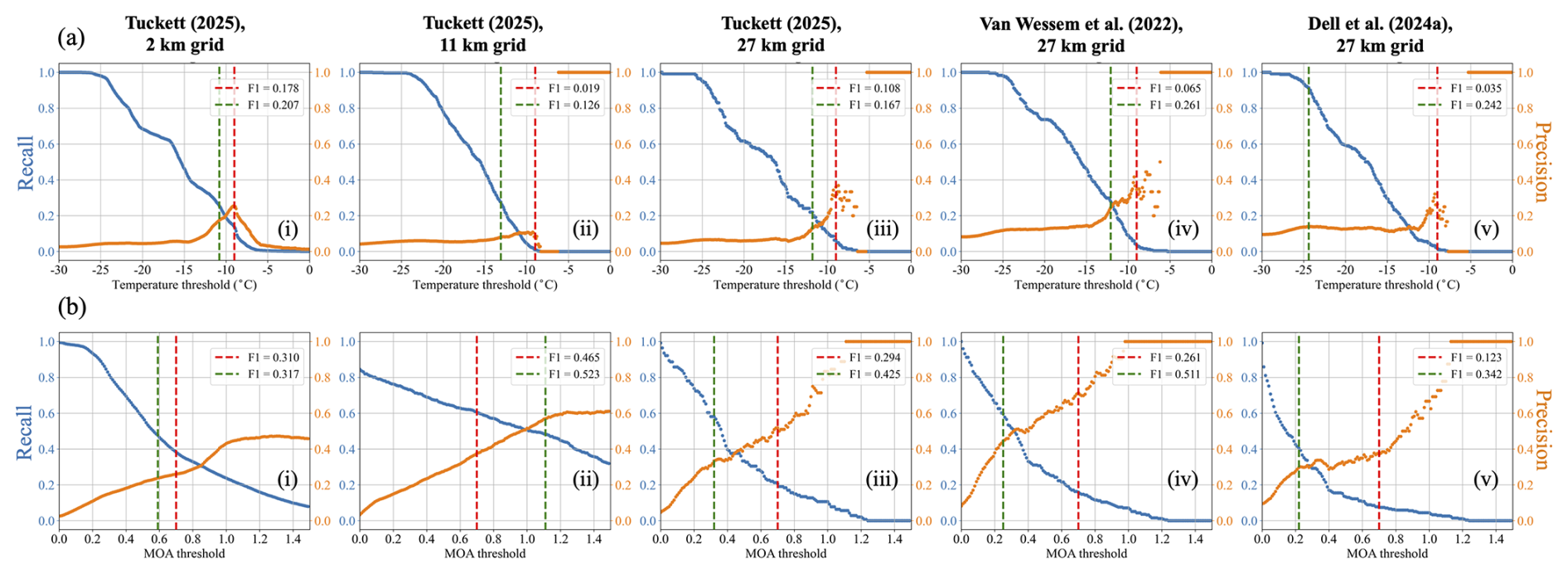
Figure A2 Recall and precision performance of temperature and MOA thresholds as predictors of surface meltwater distribution across all five comparison scenarios. Each panel shows recall (blue; the fraction of lake grid cells correctly identified as such, i.e., TP $/$ (TP + FN)) and precision (orange; the fraction of presumed lake grid cells that were correctly identified, i.e., TP $/$ (TP + FP)) as a function of (a) temperature or (b) MOA for the entire Antarctic Ice Sheet. Results are shown for lakes datasets from Tuckett et al. (2025) at 2, 11, and 27 km resolutions (i, ii, iii), van Wessem et al. (2022) at 27 km resolution (iv), and Dell et al. (2024a) at 27 km resolution (v). The red dashed lines denote the location of the literature-based thresholds, −9 °C (temperature) or 0.7 (MOA), and the green dashed lines denote the location of the optimal thresholds for each comparison scenario, along with the corresponding F1 scores.

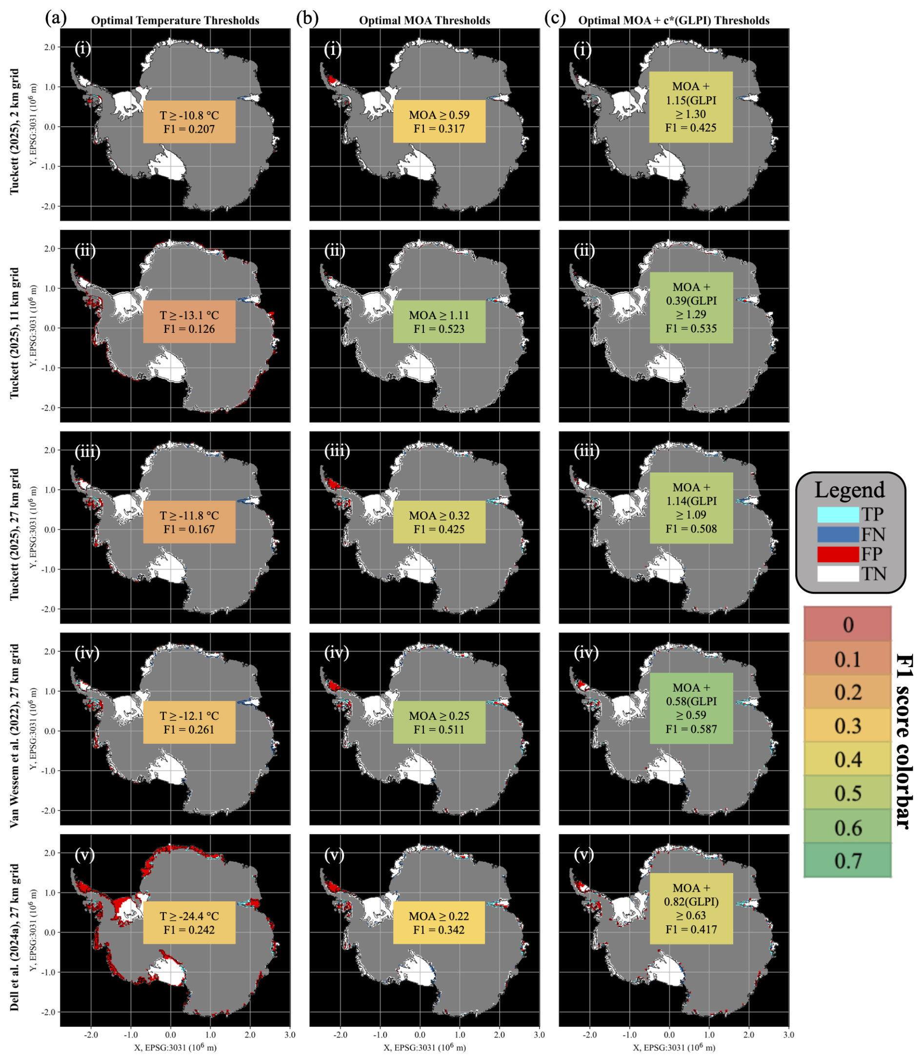
Figure A3 True positive, false negative, false positive (TP/FN/FP) masks for all five comparison scenarios across all Antarctic ice-shelves. Results are shown for the optimal continent-wide thresholds based on (a) temperature, (b) MOA, or (c) combined MOA and GLPI, for scenarios (i) Tuckett-2k, (ii) Tuckett-11k, (iii) Tuckett-27k, (iv) VW-27k, and (v) Dell-27k. For each region and threshold type, ice-shelf grid cells are colored to indicate true positives (light blue; correctly identified lake grid cells), false negatives (dark blue; observed lake grid cells not captured by the threshold), false positives (red; dry grid cells incorrectly classified as lakes), or true negatives (white; correctly identified dry grid cells). The red-green color scale of the overlying text boxes represents the value of the F1 scores, and is consistent amongst Figs. 6, 7, and A3.

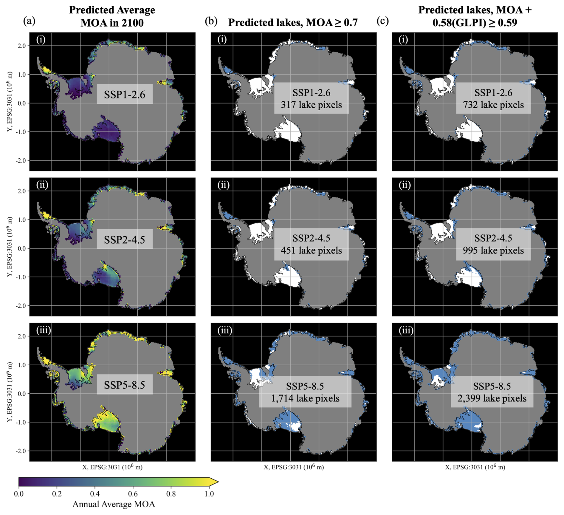
Figure A4 Projections of MOA and lake distribution in 2100 under three emissions pathways across all Antarctic ice-shelves at 27 km resolution. Columns (a)–(c) show (a) projected annual average MOA from 2090-2099, (b) projected surface meltwater distribution based on the theoretical threshold of MOA ≥ 0.7, and (c) projected surface meltwater distribution based on the empirical continent-wide threshold of MOA + 0.58(GLPI) ≥ 0.59, under emissions pathways (i) SSP1-2.6, (ii) SSP2-4.5, and (iii) SSP5-8.5. MOA projections are derived from RACMO2.3p2 climate model outputs (van Wessem et al., 2022).

Appendix B: Observational and model data

B1 Regional climate model: RACMO

In order to determine temperature and calculate MOA, we used outputs of 2 m air temperature, meltwater production, total precipitation, snowfall, rain, and sublimation from the hydrostatic regional climate model RACMO at 27, 11, and 2 km resolutions. We also examined skin temperature in comparison with 2m air temperature, and found that the values did not result in meaningfully different optimal thresholds or F1 scores. We chose to focus on air temperature for this study to maintain consistency with the work of Morris and Vaughan (2003) and Cook and Vaughan (2010). RACMO combines atmospheric dynamics from the High Resolution Limited Area Model (HIRLAM, Und'en et al., 2002) and the European Centre for Medium-Range Weather Forecast (ECMWF-IFS, 2025), coupled with a multilayer snow model, snow albedo scheme, and drifting snow scheme (van Wessem et al., 2018).

For our coarsest resolution analysis, we used outputs from an iteration of RACMO2.3p2 (van Wessem et al., 2018) run at 27 km horizontal resolution over the entire Antarctic Ice Sheet, forced at the lateral and ocean boundaries by ERA5 reanalysis data every 6 hours (van Wessem et al., 2022). This same RACMO iteration was used in van Wessem et al. (2023) in their qualitative analysis of the MOA threshold. We used annual outputs spanning 1979 to 2022, to capture the potentially multi-decadal process of firn-air depletion. Also mirroring van Wessem et al. (2023), we used modeled projections out to 2100 forced by the Community Earth System Model Version 2 (Danabasoglu et al., 2020) from three different future emissions pathways: SSP1-2.6, SSP2-4.5, and SSP5-8.5.

We also used outputs from an iteration of RACMO2.4p1 run at 11 km horizontal resolution over the ice sheet. This version included updates to the atmospheric dynamics and an updated blowing snow scheme (van Dalum et al., 2024a), and was found to outperform RACMO2.3p2 at estimating sublimation and surface meltwater production (van Dalum et al., 2025). We obtained monthly outputs spanning 1979 to 2023.

For our highest resolution analysis, we used a statistically downscaled version of RACMO2.3p2. Coarse climate model grids often underestimate surface mass balance (SMB) because they cannot resolve complex topography, which influences foehn wind patterns (Datta et al., 2018, 2019), or local albedo, which influences surface melt (Antwerpen et al., 2022; Lenaerts et al., 2017). To address this, Noël et al. (2023a) downscaled RACMO2.3p2 outputs from a 27 km grid to a 2 km grid by incorporating high-resolution surface topography from the Reference Elevation Model of Antarctica (REMA, Howat et al., 2019) and an albedo map derived from the Moderate Resolution Imaging Spectroradiometer (MODIS). This higher resolution data product revealed higher surface melt rates, especially near the grounding line (Noël et al., 2023a). The downscaled model's SMB better matches in-situ observations of accumulation and satellite records of melt production (Noël et al., 2023a; Trusel et al., 2013; Wang et al., 2021). We obtained this downscaled RACMO product at 2 km resolution, with annual outputs spanning 1979 to 2023.

With all three resolutions of RACMO, we used Eq. (1) to calculate the annual average MOA at every grid cell. If rain was not provided as an output, it was calculated as precipitation – snowfall. Panels (i) and (ii) of Fig. 1 show RACMO2.3p2 27 km outputs of average air temperature and annual average MOA over selected regions, and Appendix Fig. A1 shows the same outputs from all three RACMO iterations.

B2 Surface meltwater distribution

To compare climate variables with the present-day distribution of surface meltwater, we used three lakes datasets representing two different mapping approaches. Two datasets, from van Wessem et al. (2022) and Tuckett et al. (2025), use threshold-based pixel identification applied to Sentinel-2 and Landsat imagery, respectively. The third dataset, from Dell et al. (2024a), applies a machine learning-based approach to classify meltwater from Landsat 8 data.

Moussavi et al. (2020) developed a threshold-based algorithm to identify pixels that represent surface water, ice, rock or seawater, or clouds in Landsat 8 and Sentinel-2 imagery. The algorithm is based on individual band reflectance values, multi-band ratios including the normalized difference water index and normalized difference snow index, and band reflectance value differences. Van Wessem et al. (2023) used this algorithm to identify lake pixels in 19 213 images from the 20 m-resolution Sentinel-2 satellite record over austral summers from 2015–2022. All images examined had less than 30 % cloud cover and solar elevation angles of at least 25°. With each lake pixel, they determined the approximate water depth using a physically-based single-band algorithm from Philpot (1989). The resulting dataset (van Wessem et al., 2022) provides the observed aggregate depth of meltwater in each 27 km RACMO2.3p2 grid cell observed by Sentinel-2 over the seven-year span. Grid cells with less than 20 mm of total observed meltwater depth were recorded as having no meltwater. For the purpose of directly evaluating the lake distribution predictions that are discussed in van Wessem et al. (2023), we use their lakes dataset as is.

While the Moussavi et al. (2020) method is shown to have high accuracy (> 95 %) in identifying lakes Antarctic-wide, it can yield false positives in areas of shadows, crevassing, or blue ice (Corr et al., 2022; Tuckett et al., 2025). To address this, Tuckett et al. (2025) slightly modified the method, increasing the threshold for the difference between green and red band reflectance from > 0.07 to > 0.10. This adjustment eliminated misclassifications of rock or cloud shadow while retaining correctly identified surface meltwater. After showing that the Moussavi et al. (2020) approach also performed well on Landsat 7 imagery (Tuckett et al., 2021), Tuckett et al. (2025) applied their modified pixel identification algorithm to all available Landsat 7 and 8 images with solar elevation angles of at least 20° from 2006 to 2021 (133 497 images in total). In order to account for limited visibility due to cloud cover and variable optical image coverage between regions, they applied an image visibility assessment to extrapolate the observed lake extent each month to an estimated maximum lake extent (Tuckett et al., 2021, 2025). They ultimately provide a 30 m-resolution map of the annual recurrence frequency of surface meltwater continent-wide, i.e., the number of years between 2006 and 2021 when each pixel was identified as a lake (Tuckett, 2025). We aggregated this frequency map onto 2, 11, and 27 km grids to match the grids of our three RACMO products. This aggregation was done by assigning each high-resolution pixel to a RACMO grid cell based on its coordinates. For each RACMO cell, frequency values from all contributing 30 m pixels were summed, and the number of contributing pixels was recorded. We divided the summed frequency values by the total number of ice-shelf pixels contained within each grid cell to produce a normalized lake presence value for comparison.

Another known problem with the Moussavi et al. (2020) algorithm is its tendency to miss shallower meltwater (≲ 0.1–0.5 m) and slush (saturated snow or firn) in its meltwater classification, as the spectral signatures of these features are similar to those of snow and blue ice (Corr et al., 2022; Dell et al., 2022, 2024b; Moussavi et al., 2020). We therefore also tested a data product from Dell et al. (2024a), who used a supervised classification algorithm to derive meltwater extents from Landsat 8 imagery (Dell et al., 2022). This algorithm used k-means clustering to create training classes for a random forest classifier, which was used to identify lakes and slush across the ice sheet. While no prior study has directly compared these three lakes products, Dell et al. (2024b) found that their machine learning-derived meltwater extents were approximately double those from earlier threshold-based methods. Dell et al. (2024b) provided continent-wide lakes data in the form of 30 m resolution “heat maps”, which indicate the number of months during the study period (austral summers, November to March, from 2013–2021) during which each pixel was identified as a lake by the algorithm. We aggregated these heat maps onto the 27 km RACMO 2.3p2 grid using the same binning method as described above for the Tuckett et al. (2025) data, and again divided the heat values by the total number of ice-shelf pixels contained within each grid cell to produce a normalized lake presence value for each grid cell.

With each of our five aggregated lakes datasets – Tuckett (2025) at 2, 11, and 27 km resolutions, van Wessem et al. (2022) at 27 km resolution, and Dell et al. (2024a) at 27 km resolution, we retained only the grid cells overlapping the total ice-shelf extent, represented as the combined maximum extent of ice-shelf shapefiles from MEaSUREs v.2 (Mouginot et al., 2017) and Dell et al. (2024a). In clipping the data, we added a buffer around the ice-shelf extents of size $r/\sqrt{\mathrm{2}}$, where r is each respective grid resolution, allowing us to capture all grid cells that at least partially overlap with the floating ice area. The areal extent of the Dell et al. (2024a) data is slightly smaller than that of the other datasets, because their data is provided separately for each individual ice shelf using slightly more constricted shapefiles, whereas van Wessem et al. (2022) and Tuckett et al. (2025) provide broader coverage.

We converted our aggregated lakes datasets into binary products by defining lake coverage thresholds at which we would consider each grid cell a “lake” location. For the Tuckett data products, we used a normalized lake presence threshold of $\frac{\mathrm{1}}{\mathrm{15}}$ (∼ 0.067). This value could represent, for example, ∼ 6.67 % lake coverage sustained across all observed years, or total lake coverage for only one of the fifteen years. For VW-27k, we used a threshold of 20 mm of aggregate meltwater depth over austral summers from 2015 to 2022, following the process of van Wessem et al. (2023) in their Extended Data Fig. 3. For Dell-27k, we used a normalized lake presence threshold of 0.1. This value could represent 10 % lake coverage sustained across all observed months or, since the Dell dataset includes five melt-season months per year for eight years (forty months total), a normalized lake presence of 0.1 could also correspond to half of a grid cell being covered with lakes for one of the five observed months each summer, i.e., $\mathrm{1}/\mathrm{2}\cdot \mathrm{1}/\mathrm{5}$ = 0.1. With these thresholds, 4.6 % of ice-shelf grid cells in Tuckett-27k, 8.5 % in VW-27k, and 9.6 % in Dell-27k are classified as lake locations. The binarized VW-27k meltwater product over selected areas is shown in the (iii) panels of Fig. 1, and the Tuckett products at all three resolutions are shown in Appendix Fig. A1. Figure 4 compares the Tuckett-27k, VW-27k, and Dell-27k meltwater products over selected areas.

Appendix C: Adjusted meltwater-over-accumulation (MOA) calculation for negative values

As the climate continues to warm, MOA values are generally expected to increase across Antarctica as the rate of increase in meltwater production outpaces that of snowfall (Donat-Magnin et al., 2021; Palerme et al., 2017; Trusel et al., 2015; van Wessem et al., 2023). However, in certain regions, an increase in sublimation with temperature may result in a net removal of snow and firn, and therefore negative MOA values (see Eq. 1). While this process could effectively precondition a region for meltwater ponding, the corresponding negative MOA values are unphysical under the current formulation and do not predict ponding under theoretical or empirical MOA thresholds.

We therefore propose a simple correction to the MOA calculation only for regions of net negative accumulation: instead of the ratio of total liquid water to net snow accumulation, as in Eq. (1), MOA could be calculated as the ratio of rain and total snow removal (due to both melting and sublimation) to snowfall. The proposed adjusted MOA is calculated as follows:

$$\begin{array}{}\text{(C1)}& {\mathrm{MOA}}_{\mathrm{adj}}=\left\{\begin{array}{l}\frac{\mathrm{snowmelt}+\mathrm{rain}}{\mathrm{snowfall}-\mathrm{sublimation}},\mathrm{snowfall}-\mathrm{sublimation}>\mathrm{0}\\ {\displaystyle \frac{\mathrm{snowmelt}+\mathrm{rain}+\mathrm{sublimation}}{\mathrm{snowfall}}},\mathrm{snowfall}-\mathrm{sublimation}\le \mathrm{0}\end{array}\right.\end{array}$$

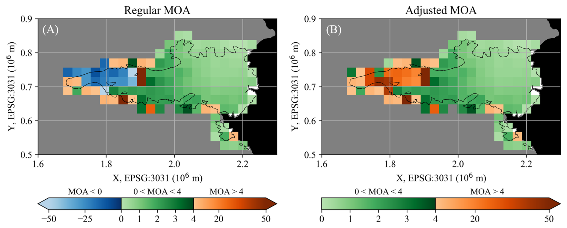
Figure C1 Projected regular and adjusted MOA over the Amery Ice Shelf in 2100 under SSP5-8.5 at 27 km resolution. (a) “Regular” MOA, calculated following Eq. (1) as the ratio of total liquid water production to net snow accumulation. (b) “Adjusted” MOA, in which negative MOA values are recalculated following Eq. (C1), as the ratio of total snow and firn removal to snowfall. Blue, green, and orange color regimes denote negative MOA values, moderate MOA values (0 ≤ MOA ≤ 4), and high MOA values (MOA ≥ 4), respectively. Future MOA values are based on modeled projections from van Wessem et al. (2022).

Figure C1 shows projected MOA values over the Amery Ice Shelf in 2100 under emissions pathway SSP5-8.5 (van Wessem et al., 2022). In Fig. C1a, we see MOA calculated according to Eq. (1), resulting in negative values in the northwest corner of the ice shelf where sublimation is expected to exceed snowfall in magnitude. In Fig. C1b, we see MOA calculated according to Eq. (C1). This results in regions of net negative accumulation having very high MOA values, which would result in predicted ponding under any reasonable threshold. At 27 km resolution, this adjustment to MOA applies to just 18 grid cells, mostly concentrated on Amery, for projections from SSP5-8.5 for the year 2100. However, it may become increasingly important for ponding predictions beyond 2100, if rising temperatures continue to increase sublimation beyond predicted snowfall.