Evaluating surface mass balance variability from climate models using GPS Bedrock Vertical Time Series data

Accurate estimates of Antarctic Surface Mass Balance (SMB) are essential for quantifying ice-sheet mass changes and their contributions to global sea level rise. Regional Climate Models (RCMs) and atmospheric reanalyses provide SMB products that are widely used in glaciology and climatology studies, yet substantial discrepancies between models persist. This study evaluates interannual to decadal variability in seven SMB models by comparing computed SMB elastic vertical bedrock displacements with GPS vertical timeseries from across Antarctica. The models vary in spatial and temporal resolution: RACMO2.3p2 (27 km), RACMO2.4p1 (11 km), statistically downscaled RACMO2.3p2 (2 km), MAR (35 km), GEMB (10 km), HIRHAM5 (12.5 km) and MERRA2 (12.5 km). Model performance is assessed through the quantification of low-frequency variance reduction in GPS residuals after SMB loading correction and by computing scale factors between the observed and model time series. Results indicate that all considered SMB models reduce long-period (>1.5 years) GPS variance on average, but performance varies across Antarctic regions and GPS sites. All RACMO variants, specifically the higher-resolution variants (2 and 11 km) show better performance overall, achieving typically the largest variance reductions and yielding scale factors closest to unity, particularly in the Antarctic Peninsula and coastal margin of Antarctica; MERRA2 and HIRHAM5 have the weakest overall performance. Our findings suggest that GPS observations, with some limitations, provide a useful new constraint on SMB model evaluation that yields insights into spatial and temporal variabilities that traditional SMB model evaluations are unable to fully resolve.

1 Introduction

Antarctic Surface Mass Balance (SMB) products derived from regional climate models (RCMs) and atmospheric reanalyses are used in a wide range of climate and sea level studies. These include quantification of ice-sheet contribution to sea level using the input-minus-output approach (e.g., Rignot et al., 2019), climate variability analysis (e.g., Dalaiden et al., 2020; Macha et al., 2025), input into modelling firn densification (e.g., Ligtenberg et al., 2011), Glacial Isostatic Adjustment (GIA) modelling (e.g., Willen et al., 2020) and technical studies of satellite geodetic observations (e.g., Koulali et al., 2022; Martín-Español et al., 2016). Thus, it is important to gain confidence in the accuracy of such models, particularly in their ability to capture SMB temporal variability.

However, comparisons between different SMB models show significant discrepancies over different spatial and temporal scales (Mottram et al., 2021). These differences largely arise from uncertainty in the appropriate way to represent the various Antarctic climatological processes, including SMB processes, limitations in their implementation in the model, and errors in large-scale forcings (Lenaerts et al., 2019; Mottram et al., 2021; Seroussi et al., 2020). Observations to inform such Antarctic surface processes, including the modelled SMB, are spatially and temporally sparse (Mottram et al., 2021; Vandecrux et al., 2025; Wang et al., 2025). Such uncertainties in SMB propagate into contemporary long-term ice-sheet mass change estimates obtained from satellite-based input-output methods and, in some cases, satellite altimetry, where firn densification models are used to convert elevation changes into mass changes (Ligtenberg et al., 2011; Otosaka et al., 2023; Rignot et al., 2019).

To assess the performances of SMB models, three approaches are primarily employed: (i) direct validation against ice core data (Cavitte et al., 2020; Mottram et al., 2021; Wang and Xiao, 2023), (ii) inter-model performance comparisons (Mottram et al., 2021; Wang et al., 2025) and, less commonly, (iii) comparisons with satellite altimetry measurements (Verjans et al., 2021). Although each method provides unique insights into model behaviour, they are collectively constrained by limitations in spatial representativeness, temporal resolution and their own systematic or random measurement errors.

Bedrock fixed Global Positioning System (GPS) observations, with daily sampling and an expanding spatial coverage across Antarctica (Buchta et al., 2024), offers a promising complementary approach for validating SMB products. To date, GPS vertical velocity estimates of bedrock motion have mainly been used to test models of Glacial Isostatic Adjustment (GIA) after first accounting for the effects of elastic loading displacements associated with recent ice-mass changes, including SMB (e.g., Hattori et al., 2021; King et al., 2012; Thomas et al., 2011). However, recent studies have shown different models of SMB-driven elastic Earth displacements have varying degrees of agreement with regional-scale GPS displacement time series, indicating an ability to separate SMB model performance through comparison to such GPS time series (King et al., 2022; Koulali et al., 2022, 2025).

In this study, we use non-linear vertical bedrock displacements derived from a set of Antarctic GPS position timeseries to assess the performance of a suite of SMB predictions generated within six RCMs and one atmospheric reanalysis dataset. We indirectly assess the performance of the modelled SMB by comparing SMB loading displacements computed at GPS sites, using well-understood elastic Earth deformation theory (Farrell, 1972), with GPS vertical coordinate time series at a range of sites across Antarctica. We note that our objective is to evaluate the ability of GPS observations to test SMB model variability, rather than to diagnose the specific physical causes of inter-model differences, which would require a dedicated model intercomparison study.

2 Data and Method

2.1 Surface Mass Balance Loading

We use SMB products from RACMO2.4p1 (11 km spatial resolution, monthly temporal resolution; van Dalum et al., 2025), RACMO2.3p2 (27 km, monthly; van Wessem et al., 2018), a downscaled version of RACMO2.3p2 (2 km, monthly; Noël et al., 2023), MAR v3.11 (35 km, monthly; Kittel et al., 2021), GEMB (10 km, monthly; Schlegel and Gardner, 2023); forced directly with low resolution (∼ 0.25°) ERA5 reanalysis fields interpolated to the model grid), HIRHAM5 (12.5 km, monthly; Hansen et al., 2024) and MERRA-2 (12.5 km, 5 d; Medley et al., 2025). In addition to different spatial resolutions, these models have different approaches to implementing large-scale climate forcing, have different parameterisations of SMB processes, and different underlying topographic models that are then sampled at the specific model's spatial resolution. The latter differences can lead to systematic divergence in orographically driven precipitation patterns, particularly over complex terrain. These all contribute to inter-model variability.

We generated the SMB mass variability time series spanning 1980–2022 by first computing, for each SMB model, the SMB anomalies from the long-term mean SMB computed over 1980–2022 reference period (see Table S1 in the Supplement). The loading variability is not particularly sensitive to the choice of reference period provided it is multi-decadal.

Since we wish to work with mass rather than rates of mass, the resulting SMB anomalies were cumulatively summed, detrended, and bilinearly interpolated onto a common regular grid of 2 km resolution. A uniform land mask (Mosaic of Antarctica version 2; Haran et al., 2021), defining the extent of the grounded ice sheet (including the offshore islands), was applied to the grid after resampling to the same 2 km resolution (Haran et al., 2021; Mottram et al., 2021). Interpolation of coarse SMB grids is important as SMB variability over the ocean or floating ice does not impose a crustal loading signal. Interpolation onto a common high-resolution grid avoids introducing loading computation errors due to low resolution coastline definitions, with our choice matching the native resolution of the highest-resolution product considered. While bilinear interpolation results in necessarily distributing signal smoothly, the elastic loading response at a GPS site integrates SMB contributions over spatial scales of several hundred kilometres (Fig. 1).

Figure 1 Example spatial SMB variability and elastic deformation contributions at Casey (CAS1) site in East Antarctica. (a) Vertical elastic response at any GPS site to a known unit load (1 m uniform water equivalent, 1 km radius) as a function of distance. (b) IQR of SMB (mm w.e.) on 2 km grid cells in the vicinity of CAS1. (c) Spatial contribution from the load signal (as per panel b) to the vertical deformation (mm) at CAS1 site. (d) Profile of vertical deformation contributions from SMB load variability around CAS1, binned over distances up to 300 km.

To compare the different SMB models with each other and quantify their level of spatial agreement, we computed the average low-frequency coherence of the models in the frequency domain. Since the GPS time series are known to contain some systematic errors such as due to orbital errors, residual atmospheric and non-tidal ocean loading and aliasing effects at long (seasonal) periods (Blewitt and Lavallée, 2002; Penna and Stewart, 2003), we focus the comparison with the SMB models on periods longer than 1.5 years. This is not problematic as the low frequency component of cumulative SMB is the largest (King and Watson, 2020), and hence has the largest impact on GPS time series. The 1.5-year cutoff therefore attenuates aliased periodic signals while retaining the most meaningful and dominant SMB-driven loading variability.

To compute the coherence, we first isolated the long period (>1.5 years) cumulative SMB by applying a 4th order Butterworth low-pass filter with a −3 dB cutoff at 0.67 cycles per year. Then, for each grid cell, we estimated the pair-wise spectral coherence between each pair of SMB time series (Welch, 1967). The computed pair-wise coherence values were then binned to logarithmically spaced intervals (Tröbs and Heinzel, 2006), at 0.67 cycles per year corresponding to 1.5 year periods. Further, we averaged coherence within each bin and formed a single low-frequency summary by taking the arithmetic mean across log-spaced bins.

To enable comparison with the GPS coordinate time series, we computed elastic displacements derived from each of the SMB models. To do this, we converted the detrended SMB mass anomalies at each location and time into arrays of cylinders defined with 1 km radius and a height representing the equivalent ice mass. These arrays were subsequently input into the Regional ElAstic Rebound calculator (REAR, v1.5, Melini et al., 2015), adopting the Preliminary Reference Earth Model (PREM) (Dziewonski and Anderson, 1981) to compute the elastic loading displacements in a centre-of-solid Earth (CE) reference frame at each GPS site location (Blewitt, 2003). The GPS time series at non-secular timescales are expressed in a centre-of-figure (CF) frame, and thus a small inconsistency exists between the modelled loading displacements and the GPS displacement series. However, previous studies have shown that the CE frame approximates the CF frame to within ∼ 2 % for non-secular signals (Dong et al., 1997), and this difference is expected to be negligible relative to the magnitude of the loading signals. Computed vertical SMB loading displacement time series (SMBL) were then interpolated to the epochs of the GPS daily time series (described below) using cubic spline interpolation.

To provide an overview of the magnitude of the deformation and the sensitivity of GPS sites as a function of distance from the load, in Fig. 1 we illustrate the spatial variability of SMB and its contribution to elastic vertical deformation at the Casey (CAS1) GPS station in coastal East Antarctica. Figure 1a demonstrates the elastic vertical response at a GPS site to a known unit surface load (1 m uniform water equivalent load of 1 km radius disk) applied at increasing distances (0–50 km). The response is maximum in the near field 0–2.5 km, with a rapid decrease in the response with distance. Figure 1b illustrates the SMB variability spatially, expressed as the Inter Quartile Range (IQR) on the 2 km grid. The largest SMB variability is observed on the eastern flanks of Law Dome, approximately 120 km east of CAS1, rather than within the 0–20 km near-field of the site. Despite the rapid decay of the elastic Green's function with distance (Fig. 1a), the spatial contribution of SMB-driven loading to vertical deformation (in mm) at CAS1 (Fig. 1c) is distributed across both near-field and far-field grid cells. When aggregated in distance bins (Fig. 1d), these contributions extend to ∼ 250–280 km from the site, with substantial input from the 120–180 km range. This example illustrates that GPS time series are expressing in part the effects of SMB variability over potentially a several-hundred kilometre radius around a GPS site. We extend this analysis to a selected set of GPS sites in Table S2, for RACMO_2DS, GEMB_10, MERRA2_12, illustrating how the balance of near-field and far-field contributions and resulting variance reduction varies across sites and models.

2.2 GPS and residual time series

To explore a wide set of regions across Antarctica, we used the GPS based vertical coordinate time series of the REGAIN reanalysis (Buchta et al., 2024) for Antarctica, which includes 286 Antarctic GPS stations, with data spanning from 1995 to 2021 inclusive. These published time series are already corrected for non-tidal atmospheric loading (NTAL) effects (Buchta et al., 2025). We focus here on the vertical component of the GPS time series as vertical surface loading displacements are typically 2–3 times larger than those in the horizontal components (Wahr et al., 2013).

GPS records in Antarctica begin at different epochs, and some end early or contain data gaps. We conducted an initial assessment of all GPS timeseries to select suitable sites based on the following criteria: data span over 3 years, a data completeness of greater than 50 %, and the absence of transient signals or other large anomalies (the distribution of GPS sites with respect to time series length is presented in the Supplement – see Table S3). A few site time series exhibit significant disturbances before ∼ 2017 due to ice accumulation inside the antenna radome and these data periods were removed prior to further analysis (Argus et al., 2014; Koulali and Clarke, 2020). The selected 98 sites, shown in Fig. 2, are mainly distributed in West Antarctica and the Antarctic Peninsula, but with a spread along the East Antarctic coastline (details of the selected sites are provided in Table S3).

Figure 2 (a) Mean annual SMB averaged across the seven SMB models for the common period 1980–2022, shown on a 2 km interpolated grid. GPS site locations are shown by brown circle and major Antarctic regions, as referred to in the text, are labelled. (b) Average pairwise SMB model coherence (unitless) at low-frequencies (periods greater than 1.5 years), computed on the same 2 km grid. GPS site locations are shown by brown circles and site names or regions discussed in the text are annotated.

With the goal of retaining REGAIN data with signal originating from solely SMBL, we also considered the effects of other surface loading displacement signals. The largest of these loading signals in Antarctica are Atmospheric Loading (ATML) and Non-Tidal Ocean Loading (NTOL). ATML (already removed from the REGAIN time series) is largely a white noise process in Antarctica, with 1–3 mm amplitude (King et al., 2022) and has limited low-frequency signal, whereas NTOL displacements have significant low-frequency signal (Santamaría-Gómez and Memin, 2015). We removed the NTOL displacements in the centre-of-figure (CF) frame to isolate the largest remaining signal, that due to SMBL (Santamaría-Gómez and Memin, 2015; Williams and Penna, 2011). We used NTOL displacements available at https://massloading.net/ (last access: 8 March 2025; Petrov, 2015) based on the MPIOM06 ocean model (Jungclaus et al., 2013) and PREM elastic Earth model (Dziewonski and Anderson, 1981). We evaluated the influence of far-field Hydrological Loading (HYDL) displacements using the GLDAS mass loading version 2.0, which accounts for global hydrological signals outside the Antarctic continent. The resulting HYDL displacements were found to be too small to produce any applicable impact on GPS vertical timeseries in the region. Finally, we generated seven residual timeseries by subtracting each of the seven computed vertical SMBL displacements from the NTOL-corrected REGAIN time series.

To investigate the non-linear vertical motions at GPS sites, we estimated vertical velocities for each GPS site using Hector v2.1 software (Bos et al., 2013). For each timeseries generated using various loading models, we first removed outliers using Hector, with a threshold of median ±2 × IQR around the modelled site motion. Since time-correlated noise and offsets can substantially affect both the inferred noise spectrum and the uncertainty of GPS velocity estimates, for each site, we evaluated multiple noise model combinations including power-law plus white noise and a Generalized Gauss-Markov plus white noise (Huang et al., 2025; Langbein, 2004). We selected the optimal noise model based on the Akaike and Bayesian Information criteria). We estimated the stochastic noise properties while estimating constant, linear, time-varying seasonal signals (Klos et al., 2017), and offsets at selected times with manual inspection based on the dates of equipment changes (i.e., antenna and receiver). Before further analysis, we removed the estimated offsets from the GPS timeseries (see Table S3).

To quantify the power spectral density and inspect the spectral component of each site's residual time series, we computed Lomb-Scargle periodograms for each site. Then, to evaluate the performance of the SMB models in reducing low-frequency noise (periods >1.5 years) in the vertical component of the considered GPS sites, we computed the integrated area of the Lomb-Scargle periodograms over periods greater than 1.5 years using trapezoidal numerical integration. Model-specific variance changes were then derived by subtracting the low-frequency variance of each SMBL-corrected spectrum from the low-frequency variance of a baseline spectrum, taken as the REGAIN-NTOL spectrum.

As an additional metric of model evaluation, we compute the time-domain scale factor of the SMB loading displacement series with the baseline series using a separate Hector analysis. This is done by including the temporally interpolated SMB loading time series as a deterministic signal (covariate) along with other parameters during the Hector analysis. Our scale factor analysis is motivated by the observation of Koulali et al. (2025) that SMB models seemed to under-predict GPS displacements in the Transantarctic Mountains over the interannual to decadal timescales in their study.

3 Results

3.1 Spatial agreement/disagreement of SMB models

Figure 2a shows the annual mean SMB, averaged across all seven SMB models. As expected, the annual mean SMB is highest along most coastal regions and across the narrow mountainous region of the northern Antarctic Peninsula. Figure 2b shows the spatial pattern of average long-period spectral coherence between the pairs of models. As indicated by high average coherence, the models have high long-period agreement around much of coastal East Antarctica and the interior of West Antarctica, with a coherence commonly above 0.8.

Mean coherence appears somewhat correlated with average SMB, with regions of high mean SMB often also having high mean coherence, presumably because regions of high mean SMB also have high SMB variability. For example, coherence is generally lower on the eastern side of the Antarctic Peninsula than the western side, where SMB is higher (Fig. 2a). A similar east-west pattern exists over Law Dome in East Antarctica. Lower coherence is seen in the inland regions of East Antarctica, including inland of the Amery Ice Shelf (Fig. 2a), the Transantarctic Mountain region and Weddel Sea sector (Fig. 2a). Smaller areas of low coherence are also evident, such as near the Denman Glacier, where the SMB variation is relatively small.

3.2 Impact of SMBL on GPS time series

We next consider the GPS vertical time series and their Lomb spectra to investigate the ability of the different models of SMB derived loading displacements to explain the observed displacements in the residual time series. Figure 3 shows results for two example sites, CAS1 and Gomez Nunatak (GMEZ; Fig. 2b). For each site, we show detrended REGAIN vertical time series corrected for NTOL (REGAIN-NTOL; grey dots), detrended time series corrected for both NTOL and SMBL (REGAIN-NTOL-SMBL; blue dots) and detrended SMBL time series for RACMO_2DS (brown dots). For visual clarity, the timeseries are displayed with small vertical offsets. At CAS1 (Fig. 3a), which has a GPS record length of more than 25 years, applying the SMBL correction using the RACMO_2DS model substantially reduces the quadratic/non-linear behaviour in the time series and provides a better model fit, as seen in the residual series over the full observation period. Figure 3b shows the corresponding Lomb-spectra obtained after subtracting different SMBL models from the baseline series. The spectra exhibit a power-law like behaviour, with an approximately linear increase in spectral power with period in log-log space. In this example, all SMB models reduce the baseline's spectral slope and power. Among the models, MERRA2_12 shows the largest power reduction at the longest periods, although this is not the case in the 10–20-year period range. Of the remaining models, RACMO_2DS shows the largest power reduction at periods longer than 5 years. We note that the larger variability in power reduction of MERRA2_12 indicates a possible mismatch in the temporal domain in the SMB model near this East Antarctic site. We also note that the different versions of the RACMO model show similar levels of performance near this site.

Figure 3c shows the time series of the GMEZ site (Fig. 2b), located in the interior of Palmer Land, an area characterised by both higher SMB and strong inter-model agreement with mean coherence $>\sim$ 0.9 (Fig. 2b). Though this site has a data span of 12 years with a percentage missing data of 37 %, all the models exhibit significant power reduction for periods exceeding 4.5 years (Fig. 3d). Koulali et al. (2022) also reported similar inter-model agreement at this GPS site based on residual WRMS reduction, although with a smaller set of models and a shorter data period. Considering the spectra (Fig. 3d), RACMO_2DS, RACMO_27 and GMEB_10 show broadly similar performance, with GEMB_10 exhibiting slightly improved performance (i.e., reduced power) across most periods. HIRHAM5_12 shows the greatest reduction of power at the longest periods, but its performance varies throughout the other periods. RACMO_11 performs much better around 3.5 years but degrades at the longest periods, whereas MERRA2_12 displays highly variable performance across different periods. From these initial example sites, it is evident that precise GPS vertical time series in Antarctica can provide some insight into the performance of various SMB models over interannual to decadal time periods.

Figure 3 (Left Panels) Detrended vertical GPS time series for the sites CAS1 (a) and GMEZ (c). Gray dots correspond to detrended REGAIN vertical time series corrected for NTOL (REGAIN-NTOL; baseline) and vertically offset from other series by +20 mm for visual clarity. Brown dots represent detrended SMBL time series from RACMO_2DS model and the blue dots correspond to the resulting time series after applying the SMBL correction (REGAIN-NTOL-SMBL), vertically offset by −20 mm. Solid blue and black lines show the linear models estimated before and after SMBL correction, respectively. Vertical red dashed lines mark the dates of identified offsets. The time series in panels (a) and (c) span different observation periods, covering 1995–2022 for CAS1 and 2010–2022 for GMEZ. (Right Panels) Lomb-Scargle spectra for sites CAS1 (b) and GMEZ (d).

We note that some GPS sites may be impacted by substantial non-SMBL signal beyond NTAL and NTOL. For instance, sites in the Amundsen Sea Embayment are likely impacted by ice dynamic changes associated with present-day ice mass loss (Barletta et al., 2018). Additionally, sites near to Erebus Volcano (e.g., CON2, CONG, MACG, etc.) may record deformation associated with volcanic activity (Grapenthin et al., 2022). Consequently, considering SMBL corrections at these sites, sometimes increases low frequency power (see Fig. S2). We also note evidence that the Northern Antarctic Peninsula may be deforming due to viscoelastic deformation driven by SMBL not just purely elastic deformation (Nield et al., 2025). We consider each of these in the analysis below and return to these points in the discussion.

3.3 Variance reduction at GPS sites

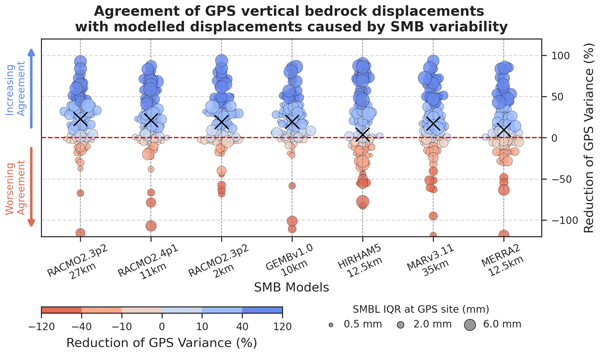
To understand the distribution of variance changes across all GPS sites for each SMBL correction, we show histograms of distributions of change in variance across all sites in Fig. 4a. All SMB models reduce the baseline GPS timeseries variance on average all sites. However, the exact response is model-dependent, and the distribution is often characterised by multiple clusters or peaks in the distribution. RACMO_27 has the largest median variance reduction of 23 %, while RACMO_11 and RACMO_2DS show median reduction of 21 % and 19 %, respectively. However, the distribution of the three RACMO variants are similar with an overall majority of sites centred between 20 %–40 %, indicating a meaningful reduction of SMBL signals at many sites when using one of the RACMO variants. Applying GEMB_10 produces a median variance reduction of 20 %. Among all the considered models, GEMB_10 and RACMO_27 show the smallest number of sites for which the application of SMB loading increases the variance (red circles, Fig. 4b). MAR_35 shows slightly lower performance than the RACMO variants, with a median reduction of around 17 %. MERRA2_12 show lower median reduction of around 10 %, with 43 % of sites clustered between −15 % to 15 %, while HIRHAM5_12 shows the weakest overall performance, with a median of only 4 %, with 44 % of sites distributed around 10 % to −20 %.

To investigate whether the magnitude of SMBL variability has any impact on the variance reduction, we repeat the distributions in Fig. 4b in the form of bubble plots, with bubble size reflecting the IQR of SMBL signal, computed over the period from 1980 to 2022, and their colours show percentage variance change (as per the y-axis). Figure 4b suggests that the change in variance is not a simple function of the amplitude of SMBL variability. Sites with larger SMBL IQR (>2 mm) exhibit a wide range of variance changes and both low and high IQR sites can show either reduced or increased variance. For example, for RACMO_2DS model there are many small blue circles indicating variance reduction of around 30 % and a few large red circles indicating variance increases exceeding 50 %. All the considered models show an increase in variance at few sites, indicated by red circles in Fig. 4b.

Figure 4 Change in variance at periods greater than 1.5 years derived by subtracting the SMB loading time series from REGAIN-NTOL vertical time series. (a) Histograms of distributions of change in variance across all sites for each SMB model. Horizontal axes span counts from 0 to a maximum of 18 sites. (b) as for panel (a), but in terms of bubble plots with marker size scaled by the site wise IQR of the SMBL. The colours used here encode the values of variance changes for better visual identification. The median of each distribution is indicated by “X”.

To aid interpretation of the impact of SMBL magnitude from different SMB models on variance changes and to assess regional variations in model performance, we analysed the percentage variance reduction by grouping the sites as a function of their respective SMBL variability and the respective change in variance for each model. We show the results for RACMO_2DS in Fig. 5, which is one of the models with overall best performance. The figures for the other models are presented in the Supplement (see from Figs. S3 to S9). Figure 5a shows the variance reduction as a function of SMBL IQR, grouped into five categories for visualisation purposes. The division of sites with stronger SMBL IQR (>2 mm) and positive variance reduction into three sub-groups: Category 1 (SMBL IQR >2 mm, VR ≥ 60 %, green), Category 2 (SMBL IQR >2 mm, 20 % ≤ VR ≤ 60 %, blue) and Category 3 (SMBL IQR >2 mm, 0 % ≤ VR ≤ 20 %, light blue). Sites with weaker modelled SMB variability (SMBL IQR <2 mm) but positive variance reductions are grouped into Category 4 (pink), while Category 5 (red) contains all sites where the model increases the low-frequency variance (VR < 0 %). Figure 5b maps the sites across Antarctica grouped into the same categories.

Figure 5 (a) Variance reduction (VR) at GPS sites as a function of SMBL IQR, using RACMO_2DS model. Colours reflect categorisation into five categories (Cat. 1–5) based on SMBL IQR (high SMBL IQR >2 mm and low SMBL IQR <2 mm) and variance reduction of the model. GPS site names discussed in the text are annotated. (b) GPS sites with colours reflecting the same categories as in (a) and symbol sizes reflecting SMBL IQR.

The spatial distribution of sites within each category exhibits regionally coherent patterns across Antarctica, with a few sites showing distinct, site-specific deviations. RACMO_2DS yields a variance reduction at almost all sites in the Southern Antarctic Peninsula with site-specific discrepancies at a few sites in the Northern Antarctic Peninsula. In Coastal West Antarctica, this model performs well, showing positive variance reduction >20 % at all but three sites (BACK, BERP and MRTP, where all other models fail to reduce variance). The model shows weak SMB signals (<2 mm) in the Transantarctic Mountains but still produces positive variance reduction at most sites, failing at only two. RACMO_2DS fails to reduce variance at most sites in the Weddell Sea sector; we note that all models struggle in this region (see Supplement for other models from Figs. S3 to S9) which we return to in the discussion. RACMO_2DS, together with the other models (except MERRA2_12), shows higher performance in variance reduction in East Antarctica, though with site-by-site model differences. In the Transantarctic Mountains, MAR_35 shows stronger SMB signals (i.e., larger SMBL IQR) than the other models and achieves good variance-reduction performance at most sites. Among the tested models, when we remove the sites where all models increase variance, RACMO_27 and GEMB_10 shows a stronger quasi-linear relationship between SMBL IQR and variance improvement (see Figs. S4 and S6).

We note that the sites grouped in Categories 2 (dark blue) and 3 (light blue), that capture comparatively stronger SMBL variability (>2 mm IQR), but showcase modest variance reduction, potentially indicate model specific limitations that would otherwise improve the variance. It is however important to note that there could be several reasons for the reduced performance at specific site locations in this category such as (i) SMB model related issues such as misrepresentation of SMB amplitude or incorrect timescales of SMB variability (i.e, misrepresented low-frequency components), (ii) systematic errors and artifacts in GPS biasing the low frequency component and (iii) mis-modelled or ignored geophysical signals (non-SMB loadings and other long-term solid Earth responses), which can mask or interfere with the SMB signals. To further understand these reasons, we show SMBL scale factors in Fig. 6, estimated for each site. Koulali et al. (2025) compared GPS and SMBL series in the Transantarctic Mountains and found that SMBL series exhibited a decadal signal broadly consistent with GPS but with reduced scale. We show the scale factors for other regions and their associated uncertainties for three example SMB models GEMB_10, RACMO_2DS and RACMO_27 for sites within Categories 1 (green), 2 (dark blue) and 3 (light blue). Scale factors greater than one indicate an under representation of SMBL amplitude, requiring upward scaling to best match the GPS residual series; less than one indicates an over-representation of SMBL amplitude.

The GEMB_10 scale factors (Fig. 6a) show high station-to-station variations with larger uncertainties, particularly across the Antarctic Peninsula and Weddell Sea sectors. Relatively large uncertainties here suggest that a SMBL has a worse temporal fit to the GPS. The weighted mean scale factor across all sites shown in Fig. 6 is 1.13 ± 0.08 for GEMB_10 (Fig. 6a), potentially suggesting an underprediction, whereas it is 1.05 ± 0.06 for RACMO_27 (Fig. 6b) and 0.95 ± 0.05 for RACMO_2DS (Fig. 6c), both insignificantly different from unity (note the uncertainties provided ±1-sigma). Within the APIS, GEMB_10 underpredicts the GPS inferred SMB variability (scale factor >1) at most sites with a weighted mean scale factor of 1.30 ± 0.10, and notable exceptions at FONP and WLCH. Comparing with the other models, the scale factors for RACMO_27 (Fig. 6b) and RACMO_2DS (Fig. 6c) are much closer to 1 with a weighted mean scale factor of 1.24 ± 0.04 and 1.10 ± 0.05 respectively in the Antarctic Peninsula. We also note that the site-by-site uncertainties of the GEMB_10 scale factors are larger in the Antarctic Peninsula, suggesting that the temporal pattern of GEMB_10 is in worse agreement with the GPS series than the other models and this cannot be resolved simply by temporally-uniform scaling (see Figs. S10 to S12). For example, at SPRZ all three of GEMB_10, RACMO_27 and MERRA2_12 show high scale factors (>2.5), whereas RACMO_2DS, RACMO_11, MAR_35 and HIRHAM5_12 show scale factors close to 1 and exhibit larger variance reduction (>60 %). All the models have high scale factors at SGP5 and SGP1; this may reflect the short duration of available GPS records at these two sites (∼ 3 years), rather than a systematic model bias.

While the differences are not as large in other regions, between-model differences are still evident. Across East Antarctic coastal sites, most of the models produce scale factors close to 1 (with notable exception of MERRA2_12). There are, however, several sites with scale factors below 1, implying a mismatch of model amplitude; or scale factors close to one and with small uncertainties, suggesting a reasonable temporal SMBL pattern. In the Weddell Sea sector, all models show large station-to-station variability, with both positive and negative scale factors, and the fit is particularly poor at WHTM site (Fig. 5), where the scale factor exceeds 2 although with a large uncertainty (indicating a poor temporal fit to the GPS data). In coastal West Antarctica the scale factors are less than 1, indicating that SMB models have reasonable temporal coherence with GPS.

Figure 6 Scale factors and associated uncertainty estimated for (a) GEMB_10, (b) RACMO_27 and (c) RACMO_2DS models grouped by geographical region. The size of the markers indicates the respective SMBL IQR and the colours indicates the categories of the sites, both as per Fig. 5. Error bars indicate a 1-sigma uncertainty. The horizontal dashed line marks a scale of 1.

4 Discussion

Koulali et al. (2022) studied time-varying elastic signals in GPS vertical displacement time series driven by SMB at GPS sites in the Southern Antarctic Peninsula. They showed that the higher resolution RACMO2.3 (5.5 km) performed better compared to RACMO_27 and MAR_35 and suggested this was due to greater sensitivity of accumulation patterns to local topography in higher resolution models. Similarly, King et al. (2022) and Koulali et al. (2025) showed that accounting for SMB related elastic loading is important when deriving long-term vertical velocities across different Antarctic regions. Building on these findings, we assessed the ability to use GPS observations for evaluating different SMB models.

Our GPS-based evaluation of SMB models provides an integrated observational constraint on SMB-driven elastic loading. Because the GPS loading signal reflects the combined effects of SMB variability over both space and time, our analysis evaluates the ability of each model to reproduce the integrated space-time variability recorded by the GPS network. While this complicates attempts to understand the origin of the mismodelled signal, careful analysis of the time series differences and the spatial pattern of SMB variability (e.g., Fig. 1b) provides further key insights. Given the GPS network used here is concentrated in coastal and peninsula regions, our evaluation is therefore more informative in these regions. The conclusions about the model performance in the interior of Antarctica remain comparatively under-constrained by the current network, given the small number of interior sites governed by limited bedrock outcrops.

Our results suggests that all SMB models considered are in sufficient agreement with the variability within the independent GPS bedrock vertical coordinate time series that, once subtracted from the GPS series, they reduce variance at periods longer than 1.5 years when averaged across all sites. However, the resulting level of improvement is model-, region-, site-, and time-dependent. The observed site-to-site variability is consistent with the finite spatial sensitivity of GPS, whereby each site responds to spatially-weighted integral (i.e., Fig. 1a) of temporally varying surface mass changes over near-field to far-field regions (e.g., Fig. 1c). Consequently, inaccuracies in far-field SMB can still exert a strong influence on estimated variance reduction and scaling. Thus, part of the model- and site-dependent performance depends on how well each SMB model captures accumulation patterns within the full sensitivity radius of any specific GPS station.

We find that all RACMO variants achieve substantial reductions in low-frequency GPS variance and yield scale factors closer to unity across much of Antarctica. Among these, RACMO_2DS and RACMO_11 show best overall performance (see Fig. S9). We suspect that the improved representation of orographically modulated precipitation and surface processes in RACMO variants appears to be translated into SMB loading signals with amplitudes and temporal patterns that better match GPS-derived deformation (Noël et al., 2023; van Dalum et al., 2025). We note that spatial weighting was not applied to the computation of median variance reductions. Consequently, the underlying site distribution particularly concentrated in Antarctic Peninsula and West Antarctica should be considered when comparing models' apparent overall performance (Fig. 6). Across the APIS, RACMO_11 has improved representation of SMB compared to RACMO_27 at many sites (see Fig. S9) (van Dalum et al., 2025). Nonetheless, the coarser-resolution RACMO_27 along with MAR_35 performs competitively in terms of continent-wide variance reduction and in the temporal representation of GPS signals indicated by the computed scale factors.

However, regional discrepancies highlight a limitation of GPS based SMB evaluation. In the leeside region of the Transantarctic Mountains, where SMB is near-zero or negative due to persistent blue ice conditions (Nowak et al., 2024), MAR exhibits comparatively better agreement with GPS-derived displacements despite being known to produce anomalously high SMB in this region (Mottram et al., 2021). From an SMB-process perspective, one would therefore expect limited temporal variability and, consequently, a weak elastic loading signal. The relatively strong performance of MAR in this region is thus somewhat counterintuitive and suggests that agreement with GPS does not necessarily imply a more realistic representation of SMB magnitude. Instead, it may reflect a compensation effect, whereby MAR's enhanced SMB variability, although likely overestimated in absolute terms, better matches the amplitude of low-frequency signals present in the GPS time series. This interpretation is consistent with our scale factor analysis and is consistent with the findings of Koulali et al. (2025), who reported similar behaviour in this region.

More broadly, this highlights an important limitation in interpreting GPS-based SMB evaluation: the method is primarily sensitive to variability rather than mean state and does not directly distinguish between physically realistic and compensating errors in SMB magnitude. In regions such as the Transantarctic Mountains where the SMB magnitude is small and spatially heterogeneous, processes such as wind-driven redistribution and sublimation dominate, even small absolute model biases can translate into relatively large differences in inferred loading signals. Consequently, improved agreement with GPS in these regions should be interpreted cautiously and in conjunction with independent observational constraints, of which there are presently few (Mottram et al., 2021). This underscores the need for combined evaluation frameworks that integrate GPS, field observations, and process understanding to better resolve SMB behaviour in low-accumulation environments.

Despite their relatively high spatial resolution, the performance of GEMB_10, MERRA2_12 and HIRHAM5_12 might be limited by differences in model formulation, including atmospheric forcing, cloud and precipitation parameterisations and treatment of snow redistribution processes (Gardner et al., 2023; Hansen et al., 2024; Mottram et al., 2021; Wang et al., 2025). For example, although the GEMB model used in this study is run and reported at a nominal spatial resolution of 10 km, its effective input resolution is forced by atmospheric fields interpolated from the ∼ 0.25° ERA5 reanalysis fields prior to the surface energy and mass balance calculations, without downscaling. Similarly, although the MERRA-2 SMB product is distributed at 12.5 km (MKR12K) resolution, it is driven by the underlying MERRA-2 reanalysis at a much coarser ∼ 0.5° × 0.625° grid making the representative resolution much larger than 12.5 km (Medley et al., 2022). Identification of the precise reason(s) for the various levels of model agreements demands a detailed study into the representation of interannual-to-decadal SMB variability (King et al., 2023; Macha et al., 2025). Accordingly, the physical origins of the differing degrees of variance reduction and the under- or over-representation of SMB variability are most appropriately examined by the developers/modelling groups of each SMB products within their context of their respective model formulations.

We note the best performing models achieve a median variance reduction of $<\sim$ 30 %, implying that a substantial fraction of low-frequency GPS variance remains unexplained across all models. A substantial portion of this residual unexplained variance at GPS sites is attributable to non-SMBL geophysical signals common to all the models evaluated, including residual mis-modelled SMB signals and unmodelled non-SMB loading signals such as varying ice dynamics, viscoelastic deformation, as well as low frequency GPS noise. These signals are not expected to be reduced by any SMB loading correction.

We also note that, as shown by Nield et al. (2025), vertical motion at several sites in the Antarctic Peninsula is better explained by a viscoelastic solid Earth response to SMB variability, rather than by a purely elastic model. Since our study assumes elastic loading only, any viscoelastic response to multi-decadal SMB anomalies will project into the low-frequency residuals, showcasing as amplitude/phase errors in these SMB products. We therefore expect that the presence of an unmodeled viscous signal would lead to scale factors greater than 1, even when the SMB estimates from the model are perfect. For example, for the RACMO_27 and MAR_35 outputs, also used by Nield et al (2025), we observe scale factors above 1, at stations that are well represented by viscoelastic models. The observed patterns of model disagreement – namely, a systematic scaling of SMB estimates and variance reduction are well explained in West Antarctica – especially in Amundsen Sea Embayment (Figs. 6 and S10). Barletta et al. (2018) indicated a low-viscosity upper mantle in this region, where an enhanced and more rapid viscoelastic response to loading is expected. Therefore, the apparent mis-scaling of SMB models and their relative variance reduction in this region could be partially attributable to this unmodelled viscoelastic component. However, Barletta et al. (2018) reported that several sites in this region show deformation consistent with present-day ice mass changes, suggesting that non-SMB related signal could also contribute to the observed scaling biases alongside unmodeled viscoelastic effects. Future work incorporating a viscoelastic Earth model would therefore be valuable for further understanding, although it introduces significant extra uncertainty in the use of GPS to test interannual variability in SMB models.

Traditional SMB observations (stakes, ice cores and radar) remain spatially sparse and temporally limited, with pronounced gaps across the Northern Antarctic Peninsula, coastal West Antarctica, Transantarctic Mountain region and coastal East Antarctica (Mottram et al., 2021; Vandecrux et al., 2025; Wang et al., 2025). Bedrock fixed, continuous GPS observations offer an additional approach with daily sampling and potentially continuous measurements that provide regionally integrated records of low-frequency SMB signals across these under-sampled regions. When combined with available in-situ and remote sensing data, these GPS constraints can strengthen SMB model evaluation and development. This underscores the value of sustained GPS station deployments to capture ideally continuous inter-annual to decadal SMB variability, in addition to its value for GIA and other geophysical studies.

A high fraction of Antarctic precipitation is associated with intense Atmospheric River (AR) events (Gorodetskaya et al., 2014; Wille et al., 2021). Antarctic daily GPS coordinate timeseries from sites located near to AR landfall locations offer the potential help quantify the rapid and intensive snowfall associated with AR events, and any subsequent redistribution or sublimation.

Several limiting factors affect the use of GPS vertical time series to evaluate SMB in RCMs. Antarctic GPS height series contain both white and coloured noise (Buchta et al., 2025; King et al., 2022) that can complicate the interpretation. In addition, GPS records in Antarctica commonly include signals unrelated to SMB, such as local mass redistribution induced by regional ice dynamics (Barletta et al., 2018). There may also be small residual errors from atmospheric and non-SMB loading corrections which can bias the low frequency signal components. In addition to this, systematic errors in GPS, such as draconitic errors (systematic artefacts occurring at ∼ 351 d period and its higher harmonics that arise from the repeating geometry of GPS satellite orbits), can introduce spurious signals at near annual periods and their harmonics (Ray et al., 2008; Tregoning and Watson, 2009). Further, operational and processing issues such as snow intrusions into the antenna radome (Koulali and Clarke, 2020), equipment degradation, uncorrected offsets and/or inaccurate offset selections further degrade the signal estimations by introducing additional offsets and spurious signals (Gazeaux et al., 2013; Huang et al., 2025). Though proper processing steps and selection criteria reduce the impact, these are not entirely eliminated. Since we assume that the dominant component of the residual variability in GPS time series is driven by SMBL, in the regions where this is invalid, we lose the ability for GPS to offer useful insights into SMB models. Across all seven models, seven sites consistently show an increase in variance and are grouped in Category 5 (red) (see Fig. S13). Generally, an increase in variance at a given site can arise from: (i) either the SMB loading signal at that site having poor temporal and/or spatial accuracy (see Fig. S2), (ii) the GPS record contains substantial low-frequency deformation that is not associated with SMBLs, such as those due to ice dynamic mass changes or volcanic activity, or (iii) the GPS time series is compromised at low frequencies due to snow intrusion into the radome or other equipment issues (Koulali and Clarke, 2020). In these cases, we note that the non-SMBL signal is dominant and hence interferes destructively with the application of SMBL time series (see Fig. S2).

5 Conclusions

We assess the performance of modelled SMB variability from seven different models across Antarctica by assessing how their inferred elastic loading signals compare to low-frequency variability in vertical GPS position timeseries. At most sites and for all models, removing SMB loading signals from GPS vertical time series reduces the low-frequency power and the spectral slope, indicating noise reduction in the residual time series. However, the response is model- and site-dependent. Overall, RACMO variants perform best, with RACMO_2DS and RACMO_11 showing the largest variance reduction and closest agreement between the modelled SMB loading displacements and GPS bedrock displacement observations. RACMO_27 and MAR_35 show comparable performances across most regions of Antarctica, except in the Transantarctic mountains, where MAR_35 outperforms all the considered models.

We find that although GEMB_10 shows a positive variance reduction across Antarctica, it fails to adequately represent SMB loadings consistent with those inferred from GPS in the Antarctic Peninsula, at least in part due to its annual sampling. MERRA2_12 and in particular, HIRHAM5_12 show notably weaker overall performance. Despite this, we present evidence to suggest that the degree of variability in even the best models does not closely match the GPS variability across few different regions of Antarctica and are often damped compared to GPS.

Overall, our results demonstrate that continuous Antarctic GPS observations provide a powerful additional dataset to evaluate SMB model performance. The approach can reveal regional strengths and deficiencies that are not necessarily captured by traditional SMB observations. Conversely, optimised SMB loading corrections such as those from RACMO variants reduce low-frequency variance by up to 60 %, yielding more reliable secular velocities for GIA and ice mass studies. With an expanded Antarctic GPS network, GPS-based evaluations could be used to improve confidence in estimates of ice-sheet mass variability and its varying contribution to sea-level change. The value of this technique can only be fully realised with long-term, continuous GPS observations at bedrock outcrops across Antarctica.