Brief communication: Shared parameterisation for estimating snow water equivalent through cosmic ray neutron sensors in the Italian Alps

We present a novel approach based on leveraging a shared parameterisation to derive snow water equivalent (SWE) with cosmic ray neutron sensing (CRNS) probes. The network comprises 26 sites (1422–2901 $\mathrm{m}\mathrm{a}.\mathrm{s}.\mathrm{l}.$) in the Italian Alps. The parameterisation was defined by fitting neutron counts to 35 SWE measurements taken at 6 sites in the first half of the 2023–2024 snow season and validated with 111 SWE data from 2023–2024 and 2024–2025 at 13 sites. Our analysis shows that this approach retains good representativeness of the snowpack. Further results show that correlations between SWE series from coupled monitored and unmonitored sites are strongly affected by elevation differences.

1 Introduction

Mountain snow is crucial for mountain ecosystems and plays a crucial role in sustaining human activities (Mankin et al., 2015). Its relevance is bound to increase as global projections estimate that in the next decades ∼1.5 billion people will be depending on mountain water runoff (Viviroli et al., 2020). The European Alps constitute the main water reservoir for millions of people (Immerzeel, et al., 2020). However, the Alpine snowpack is strongly affected by temperature increase linked to climate change (López-Moreno et al., 2020a). Snow persistence in the Alps has substantially declined in the last decades (Hammond et al., 2018) and the dates when complete snowpack waning happens in the water year are projected to be anticipated by as much as one month by the end of the century (Vorkauf et al., 2021). These circumstances exacerbate the need for accurate and widespread snow monitoring.

From a hydrological point of view, one of the most relevant variables associated with snowpack is its equivalent water mass (i.e. the snow water equivalent, SWE) (Beniston, 2012). The most common way to assess SWE involves in situ measurements campaigns where snow depth and bulk density values are taken through coring or snow pits. However, these measurements retain low time and spatial coverage since they are inherently linked to site accessibility, weather conditions, and personnel availability. An alternative method not requiring the repeated involvement of manpower during the season consists in the adoption of snow scales and snow pillows (Egli et al., 2009), although they are not well suited for deployment on the rough terrains typical of most Alpine valleys (Kinar and Pomeroy, 2015). Recently, new approaches for continuous in situ SWE measuring have emerged such as the use of lakes as natural snow scales (Pritchard et al., 2021), ground-penetrating radar (Schmid et al., 2014), and GPS signal variations (Capelli et al., 2022).

Another way to retrieve SWE data comes from cosmic ray neutron sensing (CRNS). CRNS exploits the interaction between neutrons and the hydrogen present in water molecules to give SWE estimates. The adoption of CRNS probes has gained traction with studies performed in North America (e.g. Sigouin and Si, 2016), the Himalaya (e.g. Pokhrel et al., 2024), and Europe (e.g. Gugerli et al., 2019). CRNS probes allow for great improvements in the time density of SWE datasets of already monitored sites, where manual SWE measurements can be used for their site-specific calibration (Bogena et al., 2020).

The Alps are the most extensive mountain range in Europe, spanning about 1200 km along their W–E axis while being part of eight countries. The Italian Alps make up about a quarter of the total area of the Alps and lie almost entirely south of the main Alpine watershed (Brugnara and Maugeri, 2019).

Here we present a network of 26 CRNS probes integrated into existing weather stations along the Italian Alps. We leverage the unprecedented coverage offered by such infrastructure to gain insights about its ability to depict the SWE independently on most of the site-specific features usually adopted. Indeed, the same parameterised relation between neutron counts and SWE is shared by each site of the network. We compared 146 direct SWE measurements, performed at 13 sites during the 2023–2024 and 2024–2025 snow seasons, with CRNS data to gain insights on the performances of this methodology and its potential reliability even in absence of reference manual data. Of the 146 available manual SWE measurements, we used 35 from 6 sites to calibrate and define the parameterisation.

So far, no studies have investigated the possibility of exploiting CRNS probes to retrieve continuous SWE data from sites not accessible and, therefore, lacking direct measurements needed for calibration. Moreover, to the best of our knowledge, this is the first work that explores the adoption of the same parameterisation for retrieving SWE from neutron counts among sensors placed in an elevation range of ∼1.5 km (1422–2901 $\mathrm{m}\mathrm{a}.\mathrm{s}.\mathrm{l}.$) and spanning more than 5° in longitude across the Alps. Our work paves the way for the application of CRNS technology in snow monitoring at regional scale, overcoming common criticalities such as site accessibility issues, lack of manpower to perform direct measurements, and safety hazards linked to the harsh mountain environment.

2 Data and methods

2.1 Network and station setup

Our network consists of 26 stations installed across the Italian Alps (Fig. 1), equipped with CRNS probes developed by Finapp SpA. The elevation range of the network covers almost 1500 m between the lowest and the highest stations, namely Lisser (1422 $\mathrm{m}\mathrm{a}.\mathrm{s}.\mathrm{l}.$) and Mosso (2901 $\mathrm{m}\mathrm{a}.\mathrm{s}.\mathrm{l}.$). Each sensor was integrated into already existing automated weather stations (AWSs) or, if the AWS framework could not host it, in the immediate proximity. A summary of the main features of each site (e.g. name, coordinates, elevation, number of manual SWE samples, and series length) is given in Table S1 in the Supplement. The AWSs employing the CRNS probes are managed by various institutions: the Regional Environmental Protection Agencies (ARPAs) of Veneto and Piemonte, the Office for Hydrology and Dams of the Autonomous Province of Bolzano, the University of Torino, and the Polytechnic University of Torino. The sensors are based on Lithium-doped ZnS(Ag) scintillators capable of detecting and discriminating neutrons and muons (Gianessi et al., 2024). The measurement of the local muon flux allows for an accurate site-specific correction of the neutron flux without the need of relying on a network of public observatories (Stevanato et al., 2022), which is the standard practice for CRNS technology (McJannets and Desilets, 2023).

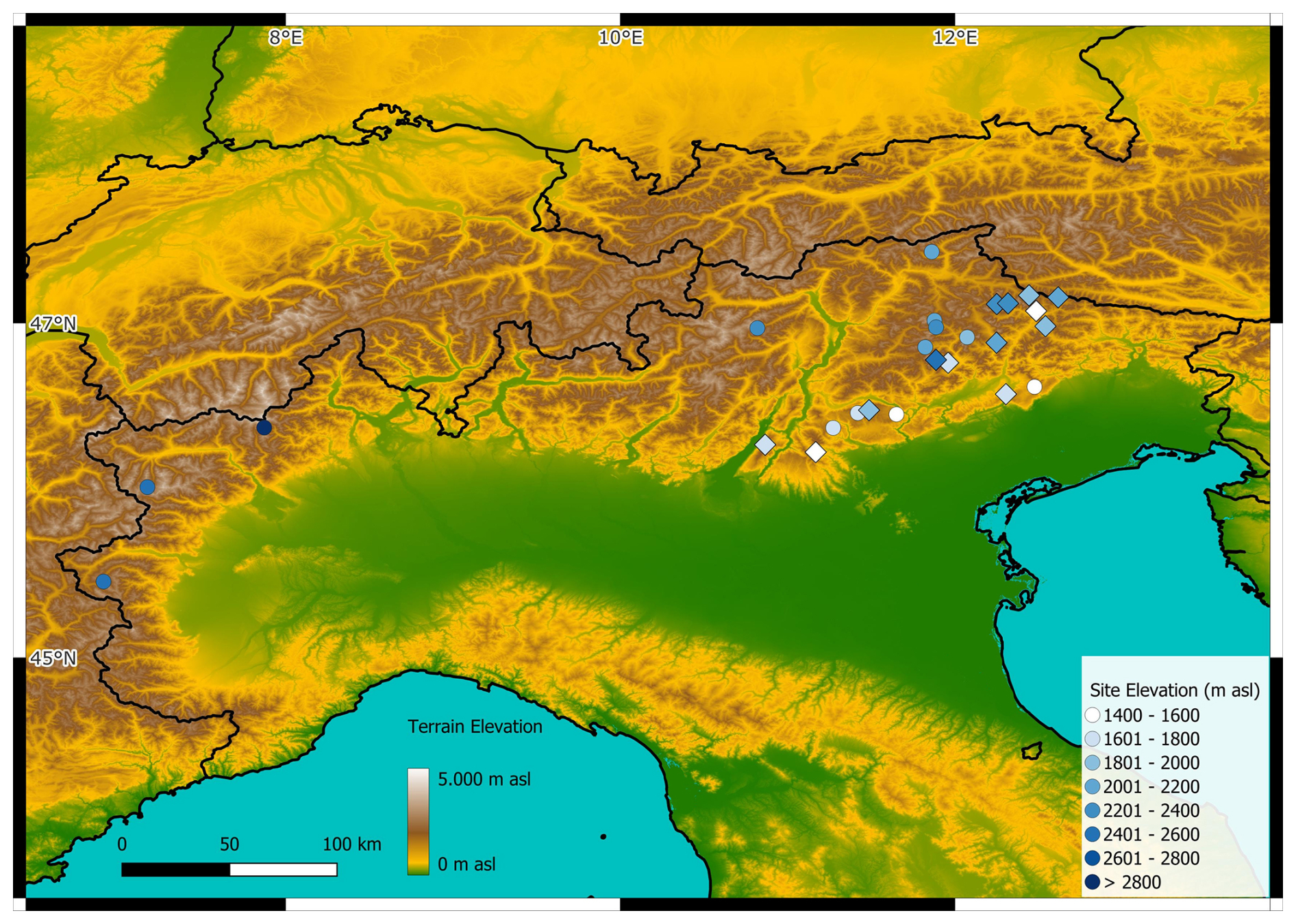
Figure 1 Elevation map of the Alps and northern Italy. Sites of the network are indicated by circles and diamonds; circles correspond to locations where manual SWE samples are available (i.e. monitored sites), while diamonds are used for location without available manual SWE samples (i.e. unmonitored sites); the symbols filling follows a scale of blue to represent the elevation of each site, where darker shades correspond to higher elevations. Produced using Copernicus WorldDEM-90 © DLR e.V. 2010–2014 and © Airbus Defence and Space GmbH 2014–2018 provided under COPERNICUS by the European Union and ESA; all rights reserved.

A CRNS setup for SWE measurement includes a detector buried flush to ground and another detector mounted on a mast, above the snow surface. The measurement footprint for this setup has a radius of approximately 20 m, a feature that allows its SWE estimates to be directly compared with point-scale manual samples.

2.2 Manual SWE sampling

At 13 sites of the network, SWE is also manually measured following two different procedures: (i) measuring the density of a single vertical core that spans the entire snowpack from the top to the ground (Berni and Giancanelli, 1966), or (ii) density measurements of multiple horizontal cores obtained from the homogenous layers present in the snowpack. In the first case, the single vertical core is weighted to derive snow bulk density and SWE. Each vertical core was taken with an Enel Valtecne EV2 corer which has an internal diameter of 6 cm and is composed by a modular setup of stainless-steel sections with a length of 50 cm each (López-Moreno et al., 2020b). The vertical coring process is repeated for at least three times for each sampling campaign, resulting in multiple SWE and bulk density values. Subsequently, those measures are averaged to obtain an estimate of the SWE. For our analysis we used these averaged values assuming they represent the (point-scale) amount of SWE at each site. In the case of horizontal coring, each core is taken with a cylinder with a volume of 0.5 dm³(i.e. length of 18 cm and diameter of 6 cm), then the core is weighted with an analogic or digital scale. If there are layers with thickness lower than the diameter of the corer, the layer density is estimated following the results of Valt et al. (2012). The measurements and, crucially, the layers identification are carried out by expert researchers and technicians who have been extensively trained by the Italian Association for Snow and Avalanches (AINEVA). The sum of the SWE computed from each core (e.g. each layer) is assumed to be the SWE of the whole snowpack. It was assessed that the differences between the two methods are within 5 % (Valt, 2018) as it has been reported in existing literature focused on snow resources of our area of study (e.g. Colombo et al., 2022; Guyennon et al., 2019). In most of the cases, the direct SWE monitoring practices pre-dates the installation of CRNS probes and the measurements were not initially meant to be used for performance assessment on this technology. This fact, in combination with the inherent spatial heterogeneity of the snowpack, could hinder the capability of such measurements of being fully representative of the actual SWE at the AWSs. This criticality descends from the absence of a defined standard for taking SWE measurements meant specifically for CRNS validation. To address this matter, we compared the snow depth (HS) measured at the AWSs with the values obtained from manual measurements. For our analysis, we discarded direct SWE measurements taken where the HS differed from the corresponding AWS value by more than 20 % for deep snowpack (i.e. HS≥1 m) or more than 20 cm for shallow snowpack (i.e. HS<1 m).

2.3 CRNS data processing and SWE computation

Each sensor retrieves raw particle counts that are integrated on a 1-h time window. The neutron count rate measured by the ground detector represents the main signal, while the muon count rate measured by the mast detector provides the incoming flux reference. To correct the raw neutron and muon counts (i.e. N_raw and μ_raw), we adopted an atmospheric pressure correction from onsite atmospheric pressure measurements (p), recorded by the barometer embedded in each probe, and applied it to obtain the atmospheric pressure corrected count rates (N_apc and μ_apc) following Eqs. (1a) and (1b):

$$\begin{array}{}\text{(1a)}& {\displaystyle }& {\displaystyle }{N}_{\text{apc}}=N_{\text{raw}}\cdot \exp \left[{\mathit{\beta }}_{\mathrm{N}}\left(p-p_{\text{ref}}\right)\right],\text{(1b)}& {\displaystyle }& {\displaystyle }{\mathit{\mu }}_{\text{apc}}={\mathit{\mu }}_{\text{raw}}\cdot \exp \left[{\mathit{\beta }}_{\mathit{\mu }}\left(p-p_{\text{ref}}\right)\right],\end{array}$$

Where β_N and β_μ are the barometric coefficients for the neutrons and muons respectively. While p_ref is the reference pressure at each site elevation (H, in meters) derived, according to the standard hydrostatic atmospheric equation (Wallace and Hobbs, 2006), as Eq. (2):

$$\begin{array}{}\text{(2)}& {\displaystyle }{\displaystyle }{p}_{\text{ref}}=\mathrm{1013.25}\mathrm{hPa}\cdot \exp \left[-\left({\displaystyle \frac{H}{\mathrm{8006}\mathrm{m}}}\right)\right]\end{array}$$

Both β_N and β_μ values used in this study were provided by the manufacturer: β_N is fixed at 0.0076 hPa⁻¹, while β_μ scales with the site elevation as described in the empirically derived Eq. (3):

$$\begin{array}{}\text{(3)}& {\displaystyle }{\displaystyle }{\mathit{\beta }}_{\mathit{\mu }}=\mathrm{0.019}\times \mathrm{0.007}{\displaystyle \frac{H}{\mathrm{10}\mathrm{000}\mathrm{m}}}\end{array}$$

The atmospheric pressure correction is a crucial step in CRNS application as the number of cosmic ray particles reaching the ground is strongly influenced by the number of particles present in the air column they cross (i.e. the atmospheric thickness), which scales with the atmospheric pressure. The choice of p_ref is arbitrary and the literature presents various instances of values fixed a priori (e.g. the standard sea level pressure of 1013.25 hPa in Bogena et al., 2022; or 1000 hPa in Jitnikovitch et al., 2021) or obtained as the median or average pressure value over a selected period of time (e.g. Gianessi et al., 2024; Gugerli et al., 2019, 2022; Stevanato et al., 2022). The rationale behind the adoption of Eq. (2) lies in the fact that the network is intended to allow for near real-time snowpack monitoring starting from the probe's installation. Therefore, the choice fell on an a priori value that could still maintain the representativeness of each site's expected average atmospheric pressure.

While performing these processing steps, we discarded data that fell under at least one of the following criteria: (i) integration time lower than 500 s; (ii) null value of either air pressure, neutron counts, or muon counts.

For each site, we took the baseline (pressure corrected) neutron and muon count rates (N_ref and μ_ref) during a period characterised by the following features: (i) minimum length of 24 h, (ii) stable signal (i.e. without probe's reboots, outliers, or evident trends that overcome the random fluctuations), and (iii) absence of snow cover. N_ref varies greatly from each site due to its dependence from elevation, soil composition, and morphology. At every station of the network, N_ref and μ_ref are assessed at the beginning of each season and their values are updated if needed.

Subsequently, to obtain the corrected neutron count (N) we applied to the pressure corrected neutron count rate (N_apc) a site-specific incoming correction factor given by the ratio between μ₀ and the atmospheric pressure corrected muon count (μ_apc) as proposed by Stevanato et al. (2022) and illustrated in Eq. (4):

$$\begin{array}{}\text{(4)}& {\displaystyle }{\displaystyle }N=N_{\text{apc}}{\displaystyle \frac{{\mathit{\mu }}_{\text{ref}}}{{\mathit{\mu }}_{\text{apc}}}}\end{array}$$

It is therefore possible to compute the normalised neutron count rate (N_r) according to Eq. (5):

$$\begin{array}{}\text{(5)}& {\displaystyle }{\displaystyle }{N}_{\mathrm{r}}={\displaystyle \frac{N}{N_{\text{ref}}}}\end{array}$$

Then, we computed SWE adopting the widely used formula (e.g. Pokhrel et al., 2024; Jitnikovitch et al., 2021; Gugerli et al., 2019; Howat et al., 2018) reported in Eq. (6):

$$\begin{array}{}\text{(6)}& {\displaystyle }{\displaystyle }\text{SWE}=-{\displaystyle \frac{\mathrm{10}}{\mathrm{\Lambda }}}\log N_{\mathrm{r}}\end{array}$$

Where the attenuation length (expressed in cm⁻¹) Λ is Eq. (7):

$$\begin{array}{ll}{\displaystyle }\mathrm{\Lambda }=& {\displaystyle }{\displaystyle \frac{\mathrm{1}}{{\mathrm{\Lambda }}_{\text{max}}}}+\left({\displaystyle \frac{\mathrm{1}}{{\mathrm{\Lambda }}_{\text{min}}}}-{\displaystyle \frac{\mathrm{1}}{{\mathrm{\Lambda }}_{\text{max}}}}\right)\\ \text{(7)}& {\displaystyle }& {\displaystyle }\times {\left[\mathrm{1}-\exp \left({\displaystyle \frac{a_{\mathrm{1}}-N_{\mathrm{r}}}{a_{\mathrm{2}}}}\right)\right]}^{-a_{\mathrm{3}}}\end{array}$$

2.4 Calibration and validation against manual samples

We assessed the parameters of Eq. (7) through a calibration process that leveraged 35 direct SWE measurements taken from six sites in the Veneto region (Eastern Alps) between December 2023 and March 2024 (Fig. S2 in the Supplement). To avoid over-parameterisation, we kept fixed the values of parameters Λ_max, a₂, and a₃. These values were taken from Gugerli et al. (2019) due to the spatial proximity of our respective study areas (the Italian and Swiss Alps). The calibration was performed on the two free parameters Λ_min and a₂. This first instance of an interpolation common to multiple sites suggested the possibility of adopting a shared parameterisation across the Italian CRNS network and prompted the study presented in this work.

We obtained (including the 35 used for the calibration) a total of 154 SWE values between the 2023–2024 and the 2024–2025 snow seasons. These measurements are assumed to be representative of the on-site SWE daily average. Therefore, to compare the coring data with the CRNS neutron count rates, we averaged the hourly values of N_r over a 24 h time span. The calibration dataset was used to define the parameters of Eq. (7) that constitute the core of the network-wide parameterisation. Then, we compared the remaining daily N_r values (i.e. the validation dataset) with the direct SWE measurements at each site. In addition, we computed the mean absolute percentage error (MAPE) to identify site-specific sensible deviations from the theoretical parameterisation. Two stations (namely Mosso and Sestriere) presented MAPEs higher than 50 % limited to the data of the 2023–24 snow season. Their sensors were installed when the snow cover was already formed. This fact prevented the standard assessment of N_ref, which had to be approximated. The efforts to define a posteriori normalisation value are ongoing, but outside the scope of this work. However, this occurrence remarks that the installation of CRNS probes needs to be performed in absence of snow cover, at least when adopting a network-wide parameterisation. To avoid biases, we decided to not consider for the next steps of the analysis the 2023–2024 data of the two stations.

After these evaluations, we converted the N_r data to average daily SWE (SWE_CRNS) according to the presented formula. For each day and site where a reference manual SWE value was available, we identified and coupled with it the correspondent SWE_CRNS. In total, we leveraged for our analysis 146 d of coupled manual and SWE_CRNS (e.g. 35 for calibration and 111 for validation). The validation dataset (Fig. S2) is divided as: (i) manual samples from the same sites chosen for the calibration, and (ii) manual samples from the 7 additional monitored sites of the network. Following the methodology adopted by Egli et al. (2009), we computed a least squares fit of the data according to the Eq. (8):

$$\begin{array}{}\text{(8)}& {\displaystyle }{\displaystyle }{\text{SWE}}_{\text{CRNS}}=\mathit{\alpha }\cdot {\text{SWE}}_{\text{manual}},\end{array}$$

We also determined the standard error (SE) of α along with the root mean square error (RMSE) of the SWE_CRNS against the manual measurements. This procedure allows us to identify the systematic bias of SWE evaluation by observing how much the value of α approaches 1 (e.g. with α=1 the evaluation is theoretically unbiased). On the other hand, SE gives a measure of how much the data are scattered along the predictive line, with the RMSE constituting an average error that can be associated to the estimated SWE values.

2.5 Correlation between time series of monitored and unmonitored sites

Finally, to address the possibility to extend our considerations to unmonitored sites (i.e. the remaining 13 sites of the network where manual SWE samplings were not available), we evaluated the correlation (r) between their SWE_CRNS series. For each of the 78 possible pairings of unmonitored and monitored stations, we computed the correlation coefficient between their N_r and SWE_CRNS time series, considering only periods where the reference AWS data showed presence of snow on the ground (i.e. HS>0 cm). We assigned the obtained correlations to different classes based on the vertical and horizontal distances between each pair of stations and computed the average correlation for each class. The chosen divisions for the vertical distances are 250, 500, 750, 1000, and 1500 m; while for the horizontal distances we chose 25, 50, 100, 200, and 500 km. We defined these divisions based on the spatial distribution of the network's sites and pursuing two goals: (i) minimize the number of void classes, and (ii) avoid classes containing only one couple of stations to make its average correlation informative. The identification of variables that influence the similarity of SWE patterns is crucial in the effort of overcoming site-specific validation. Monitored sites could act as accuracy proxy for unmonitored locations with which they exhibit high correlation. For this reason, we averaged the resulting r values among subsets depending on the horizontal and vertical distances between each couple of monitored-unmonitored sites to assess the impact of these two variables on the SWE pattern.

3 Results and discussion

3.1 Calibration and validation against manual samples

The direct SWE measurements used for the analysis range from the minimum value of 20 mm recorded at Larici site on 11 December 2024 to the maximum of 897 mm recorded at Ornella site on 4 April 2024. The median of the manually measured values is 199 mm, while for their SWE_CRNS counterparts it is 160 mm. The two series retain extremely similar distributions with interquartile ranges (IQRs) 87–335 mm for the manual and 76–334 mm for the SWE_CRNS (Fig. S3).

The values of the parameters Λ_max, Λ_min, a₁, a₂, and a₃ are 114, 21 cm, 0.41, 0.082, and 1.117, respectively. Figure 2 represents the daily averaged N_r values plotted against the direct SWE measurements for the calibration (Fig. 2a) and validation (Fig. 2b and c) dataset. The adopted parameterisation of the theoretical SWE curve appears to depict well the data distribution. R² values obtained for the calibration, validation at sites of calibration, and validation at additional sites are 0.95, 0.87, and 0.65 respectively.

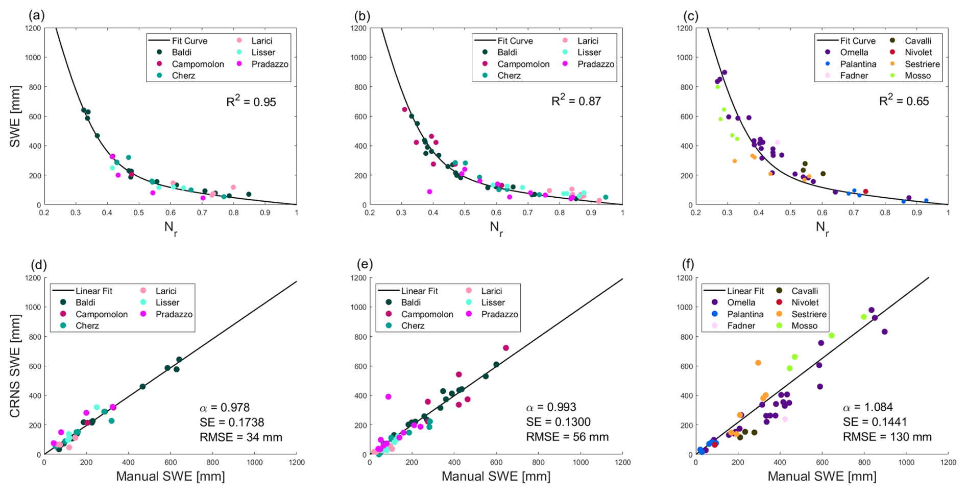
Figure 2 Normalised daily neutron count rate (x-axis) against SWE direct measurements (y-axis) for each site (coloured dots), and regression curve (black line) for the calibration dataset (a) and validation dataset divided between the six sites chosen for calibration (b) and the remaining seven sites (c). Manual SWE measurements plotted against SWE_CRNS; coloured dots represent the calibration (d), validation in the same sites as calibration (e), and validation at different sites (f) dataset respectively; the black lines illustrate the linear regression fit performed for each dataset.

Figure 2d–f presents the results of the linear regressions. The values of α suggests that the parameterization adopted does not introduce any sensible bias, as in each of the three instances of linear regression the slope is close to the ideal value 1. The SEs, which have values similar to the highest presented by Egli et al. (2009), reflect that the data are scattered along the prediction fit. We attribute this feature to two main causes: (i) the data come from different sites inherently different from one another, and (ii) the possible representativity errors introduced by the manual measurements that, we stress again, were not originally intended for this kind of performance assessment. Even considering these potentially hindering factors, the RMSE computed over the whole series is 84 mm. This result can be considered as a benchmark value when taking into account the error associated with this novel network-wide approach to CRNS parameterisation. Remarkably, both the slope and the SE obtained for the validation subset at the sites used for calibration (Fig. 2e) appear to perform better than the calibration subset (Fig. 2d). Nevertheless, RMSEs sensibly increase across the three subsets from 34 mm of the calibration subset to the 130 mm of the validation subset in the 7 additional sites. The latter subset shows also an α further from 1 (1.084) and a higher SE (0.1441).

Among the 146 analysed data, in 82 cases (22 in the calibration dataset, 60 in the validation) CRNS estimates were lower compared to the manual SWE measurements. The medians of the underestimated and overestimated manual SWE values are 168 and 209 mm, respectively. In fact, it appears that higher SWE values are more likely to be overestimated by CRNS probes. However, this result could be biased by the relative scarcity of high SWE measurements available. Indeed, more than 70 % of the manual SWE data used for our analysis have values lower than 300 mm.

To better address the site sensitivity of our network approach, we looked at the distribution of selected statistical parameters computed separately for each site. The mean absolute errors (MAEs) emerging from the comparison between SWE_CRNS data and the manual measurements have an average value of 70 mm, while the average of the site specific RMSEs is 82 mm. However, the MAE and, in a lesser way, the RMSE distributions are skewed towards lower values. In fact, the median MAE and RMSE are 47 and 67 mm. These values are comparable with the errors associated with manual SWE measurements, that increase with SWE (e.g. Gugerli et al., 2019) and can be assumed to be in the range 20–50 mm for most of the values in our dataset. Focusing on the distribution of MAPEs for each site, its average and median values are 32 % and 29 %, respectively. These values are more than double compared to the maximum percentage error of ±13 % found by Gugerli et al. (2019). However, that study involved only measurements performed by CRNS probes installed on a glacier, which cancels out possible error contributions from the underlying soil water content (Wallbank et al., 2021).

The relatively high percentage error constitutes the trade-off linked to the choice of applying the same parameterisation to every site of the network. The same choice is intended to expand the spatial coverage of continuous SWE dataset including sites that cannot be subjected to direct measurements campaigns every season due to their inaccessibility. Indeed, the only comparable European CRNS network adopts as standard procedure the seasonal recalibration through manual SWE sampling of each sensor installed (Gottardi et al., 2013). This approach, although it may yield better overall estimations in already monitored sites, limits the number of locations available for installation of CRNS probes. In any case, if needed for site specific studies, any of the SWE_CRNS dataset used for our analysis could be improved with the implementation of an ad hoc parameterisation defined using the available manual SWE data.

3.2 Correlation between time series of monitored and unmonitored sites

The correlation coefficients computed between the SWE_CRNS from unmonitored and monitored sites (Fig. 3a) appear to be influenced by the vertical distances (i.e. the elevation difference) with the average r (Fig. 3c) monotonically decreasing from a maximum of 0.87 when the distance delta is in the range 0–250 m to a minimum of 0.41 in the range 1–1.5 km. On the other hand, horizontal distances (Fig. 3d) do not seem to affect the correlation between sites. In fact, although the maximum r of 0.76 is related to the horizontal distance range 0–50 km, the minimum value of 0.67 is observed in the range 50–100 km. Unmonitored stations data are highly correlated (average r=0.98) with monitored sites with a vertical and horizontal distance lesser than 250 m and 50 km respectively. Thus, statistical behaviour of unmonitored sites, including an estimate of accuracy and representativeness of SWE measurements, can be inferred from neighbouring monitored sites in that range. An analogous analysis conducted on the Nr time series instead of the SWE_CRNS ones showed similar results (Fig. 3b). As it was the case for SWE_CRNS, the average correlation decreases monotonically with vertical distances (Fig. 3e), ranging from a maximum value of 0.83 to a minimum of 0.19. As the horizontal distance varies, the average r for the N_r time series (Fig. 3f) yields the highest value (0.78) for the 0–25 km class and the lowest (0.49) for the 200–500 km class. In absence of monitored sites meeting those characteristics, a comparison with stations at similar elevations should still yield reasonable estimates. Overall, this approach can be adopted to extend the application of CRNS to inaccessible locations further extending the spatial coverage of continuous SWE data while avoiding the necessity of an unfeasible site-specific validation.

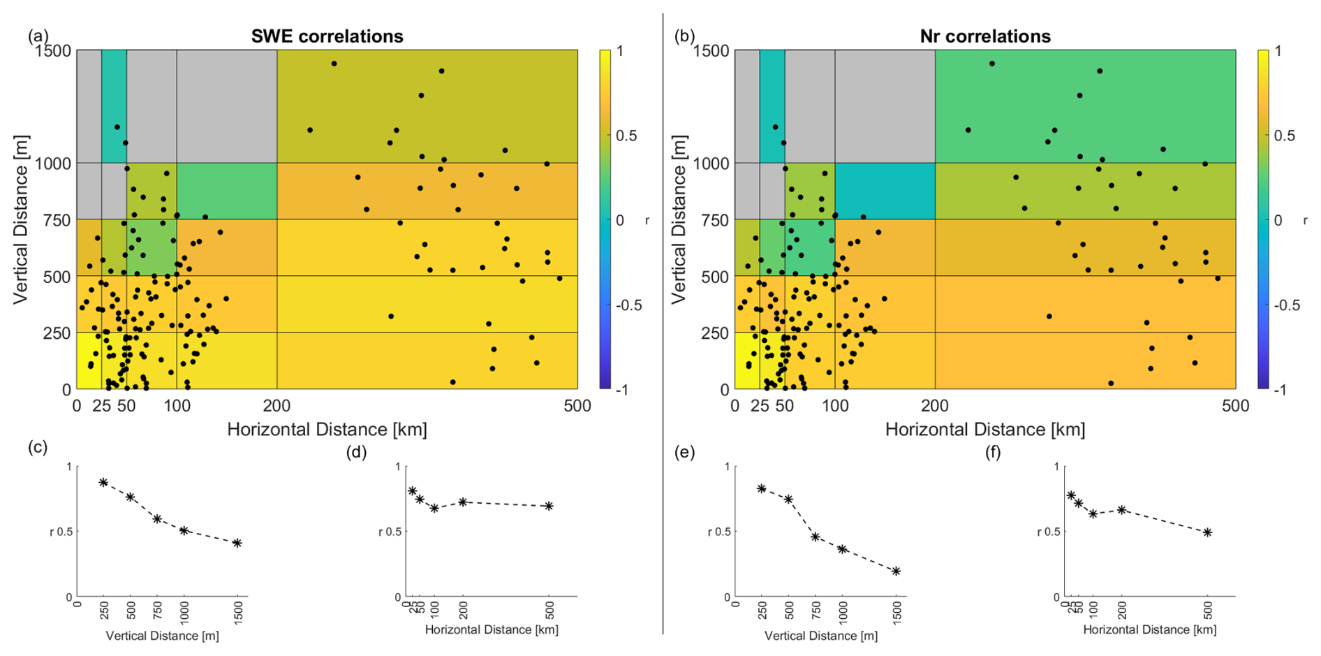
Figure 3 Heatmap of the average correlations of the SWE_CRNS (a) and N_r (b) time series classified by the horizontal (x-axis) and vertical (y-axis) distances between unmonitored and monitored stations. The black dots represent each pair of monitored-unmonitored stations for which r was computed for a total of 78 pairings. Average r values computed for each vertical (panel c for SWE_CRNS and panel e for N_r) and horizontal (panel d for SWE_CRNS and panel f for N_r) distances classes. The x coordinates of each point of panels (c) to (f) represent the upper limit of its distance class.

3.3 Limits of this study and future perspectives

The conversion of raw particles counts into SWE values depends heavily on the choice of the adopted parameters, which are the object of Sect. 2.3, and is subject to the biases that any parameterisation process introduces. In this work, we built upon what was presented in existing literature while trying to preserve the near real-time monitoring capability of the network, which demands solutions that are ready to use and representative of each site's features.

Nevertheless, we acknowledge the limitations introduced by three main factors: (i) the adoption of a single β_N for a wide elevation range, (ii) the choice of correcting the incoming neutron fluxes with muons, and (iii) the inherent variability of snowpack characteristics even at such small scales combined with the uncertainty on the footprint of CRNS probes, which may have introduced some biases in the performance evaluation of the network against manual SWE samples.

One of the main features of the network is its unprecedented elevation range. However, recent work by Davies et al. (2026), who focused on CRNS applications for soil moisture, showed that the barometric coefficient may depend sensibly on elevation. In this work, for β_N we adopted the widely accepted (e.g. Bogena et al., 2022) value of 0.0076 hPa⁻¹. Therefore, further studies shall focus on assessing the effect of an elevation dependent barometric coefficient leveraging the ∼1.5 km range offered by this network.

The most common way to perform an incoming flux correction relies on leveraging data from the nearest cosmic neutron observatory (e.g. Gugerli et al., 2019; Jitnikovitch et al., 2021). However, the CRNS probes of the network are installed with the native feature of a site-specific incoming flux correction based on muon fluxes (Eq. 4) as presented by Stevanato et al. (2022). This characteristic allows to perform a correction based solely on site-specific fluxes, although depending on a different kind of particles (i.e. the muons) which are correlated with neutrons. Nevertheless, future studies may focus on a comparison between the widely adopted correction based on neutron observatory data and the site-specific one which relies on muon fluxes.

The CRNS probes of the network retain a relatively small footprint whose radius has an upper limit of ∼20 m and is inversely proportional to the SWE. Yet, even at such scales snowpack variability plays an important role. In fact, López-Moreno et al. (2013) showed that in Alpine environments snow depth and, to a lesser extent, its density can sensibly vary for point scale measurements taken at distances of few meters thus affecting the error associated with SWE estimates. For this reason, we decided to perform comparison of manual SWE data taken where HS was comparable with the one measured by the corresponding AWS as it has been discussed in Sect. 2.2. Still, future works shall focus on the investigation how the snowpack variability affects the footprint of this CRNS setup as it has been done by Schattan et al. (2017), who focused on the above-ground CRNS assessing a footprint radius of ∼200 m although with a saturation SWE value of 500–600 mm which renders that setup unapplicable for our study purposes.

4 Conclusions

We presented a network of 26 CRNS probes integrated into AWSs covering an elevation range of ∼1.5 km in the Italian Alps that has been monitoring SWE since the 2023–2024 snow season. All probes retrieve SWE data from neutron counts leveraging the same shared parameterisation. This choice is meant to allow for reliable data collection even at inaccessible sites. As far as we know, this is the first instance of a similar feature for SWE measurements involving a CRNS network.

The comparison between the 111 validation direct SWE measurements from 13 sites showed good accordance with the conversion curve obtained through the calibration data on the same sites chosen for the calibration (R²=0.87, RMSE=56 mm) as well as in seven additional monitored sites (R²=0.87, RMSE=130 mm). The linear fit features show that this method is not prone to biases. Compared to similar studies involving a single site, the data are more scattered. We trace this back to two factors: underlying differences among the sites, and uncertainties in the manual data. Even so, the RMSE (84 mm) indicates that, even when adopting a shared parameterisation, the uncertainty of SWE_CRNS is close to the ones typical of the other methodologies presented by Egli et al. (2009). Moreover, the correlation between 13 unmonitored sites and the monitored ones shows that, across the network, SWE_CRNS patterns are strongly influenced by elevation while not being sensibly affected by horizontal distances. These results imply that uncertainties on SWE_CRNS of inaccessible sites can be inferred from stations at similar elevations, prioritising location in the 0–250 m elevation and 0–50 km horizontal ranges (average r=0.98).

Applying a network-wide parameterisation vastly expands the roster of available sites for continuous SWE monitoring. In fact, many alpine AWSs could host similar equipment resulting in accurate data regardless of the accessibility of the site and the availability of manpower. Moreover, automating data collection in the harsh mountain environment drastically lowers the exposure of workers and researchers to safety risk linked to on-site activities.

Nevertheless, we aim to expand the network as we are confident that an increase in the available data and the elevation range covered will benefit the parameterisation and its overall performances both at monitored and unmonitored sites. In this regard, future research developments should focus on three main points: (i) definition of a standardised methodology for retrieving manual SWE data specifically intended for SWE_CRNS validation; (ii) further investigation on the dependency from vertical and horizontal distances in sites comparison; (iii) assessing the impact of other local features (e.g. aspect, soil type) on the correlation between sites.