Predictability of summertime diurnal winds over ungauged mountain glaciers

Glacier and valley winds are characteristic features of the microclimate of glacierised valleys. The speed of such winds influences the turbulent heat flux, which contributes to ice melt significantly. Sparse in-situ meteorological measurements and the inability of large-scale climate data products to capture such local winds introduce uncertainty into glacier- to global-scale mass-balance calculations. Here, we propose an empirical model having three parameters, namely, the mean wind speed, the sensitivity of the diurnal winds to temperature, and a time-scale parameter, to predict the mean summertime diurnal wind speed on valley glaciers, based only on reanalysis temperature. Utilising data from 28 weather stations on 18 valley glaciers across the globe, we show that the model, driven solely by reanalysis temperature, reproduces the observed mean summertime diurnal wind speed with a mean RMSE of 0.24 m s⁻¹ across stations, which is 8.8 % of the mean observed wind speed. Interestingly, the three model parameters can be estimated even on an ungauged glacier based on the mean temperature and regional slope. A leave-one-out analysis of the stations suggests a root-mean-squared error of 0.85 m s⁻¹ on average, which is a ∼200 % improvement over a standard reanalysis product. The performance of the model is largely independent of the number of stations available for calibration, as long as it is 21 or more. The presented empirical parametrisation can improve wind speed estimates on ungauged glaciers, leading to better glacier mass-balance calculations.

1 Introduction

The microclimate of a glacierised valley has a characteristic system of local winds consisting of a glacier wind and a valley wind (e.g., Oerlemans, 2010; Broeke, 1997a, b). Glacier wind is a shallow, persistent, katabatic wind flowing down-valley. It's caused by the cooling of air by the ice surface and the associated down-slope buoyancy force (Oerlemans, 2010). Away from the glacier, as the valley floor and the hillsides are heated up during the day by solar insolation, the buoyant forces acts up-slope, leading to a daytime anabatic valley wind, which flows up-valley. It is a relatively deeper wind with a depth of ∼10² m (Nickus and Vergeiner, 1984; Vergeiner and Dreiseitl, 1987). Near the glacier termini, glacier and valley winds compete with each other at the surface level during the day (e.g., Cai et al., 2007). The buoyancy forcing in the valley, and consequently the valley wind, changes sign at night (e.g., Mannouji, 1982). This leads to a diurnal cycle of valley winds with up-valley (down-valley) flow during the day (night).

Glacier winds and valley winds fall under the general category of thermally driven slope winds (Farina and Zardi, 2023), which can be described approximately using the steady-state Prandtl model (Prandtl, 1952). This model describes the vertical profile of slope winds via a dynamic equilibrium between buoyant force and friction, and reproduces the characteristic wind speed maxima or jet at a height of a few meters above the surface (e.g., Oerlemans, 2010). During the ablation season, a linear relation between instantaneous glacier wind speed and the ambient air temperature has been empirically observed (e.g., Björnsson et al., 2005). Similar trends have also been reported for valley winds (e.g., Mannouji, 1982). This may imply that the buoyancy forces scale with the horizontal temperature gradient between the valley and the surrounding terrain (Miller et al., 2003). A simple energy exchange model was successfully used to describe the effect of katabatic cooling due to glacier wind on the variation of 2 m-air temperature along the flow-line of glaciers (Greuell and Böhm, 1998; Ayala et al., 2015).

Accurate knowledge of instantaneous wind speed on glaciers is important for energy- and mass-balance studies, as surface winds mediate energy and mass exchanges between the atmosphere and glacier surface (Cuffey and Paterson, 2010; Stigter et al., 2018). The latent heat fluxes resulting from these winds influence glacier ice sublimation rates, which can account for ∼10 %–20 % melt contribution for typical glaciers and up to 90 % contribution for glaciers in cold, arid climates (e.g., Yáñez San Francisco et al., 2025; Stigter et al., 2018). Latent heat fluxes are the dominant source of ablation for high-altitude glaciers in arid regions (Mandal et al., 2022). The net turbulent heat fluxes, which is the sum of latent and sensible heat fluxes due to these winds, can cause up to ∼10 %–35 % of the total melt on glaciers in the Himalaya (e.g., Azam et al., 2014), the Alps (e.g., Oerlemans et al., 1999), and Alaska (e.g., Klok et al., 2005). The turbulent fluxes are also important in the context of the climate response of glaciers. This is because the response of glaciers to the temperature change is largely determined by the corresponding changes in the long-wave radiation balance and those in the turbulent heat fluxes (Oerlemans, 2001). Glacier winds can affect the spatial gradients of near-surface meteorological variables such as temperature and humidity on glaciers (e.g. Shea and Moore, 2010). Simple temperature-index based methods (Hock, 1999) for estimating glacier melt involve extrapolating the near-surface air temperature for the entire glacier surface using lapse rates estimated from nearby weather stations. However, this approach can lead to overestimations of glacier melt because the air near glaciers is cooler than its immediate surroundings. The gradients of temperature, humidity, and wind speed drive heat, moisture, and momentum exchanges between valley winds and glacier winds. The presence of extensive supra-glacial debris cover favours valley winds over the ablation zone (Collier et al., 2015), which influences the glacier energy balance and the moisture transport along the valley (Lin et al., 2021).

The above discussion highlights the need of accurate wind speed estimates for glacier energy- and mass-balance studies. However, the number of glaciers where in-situ meteorological measurements are publicly available is probably of the order of ∼10² or less. This means an overwhelming majority of $\sim \mathrm{2.75}\times {\mathrm{10}}^{\mathrm{5}}$ glaciers on earth are ungauged. On these glaciers, coarse-scale reanalysis wind speed products need to be used to estimate the turbulent heat fluxes (e.g., Rupper and Roe, 2008; Rye et al., 2010). Even on the small minority of the glaciers, where weather stations are present, the data are often available for a relatively short period, or have gaps. On such glaciers, coarse-scale reanalysis data (e.g., Arndt et al., 2021; Kronenberg et al., 2022) have to be used in conjunction with the weather station data. The coarse ≳10 km resolution reanalysis products do not capture local-scale winds, and heavily underestimate their speed, and therefore, the associated turbulent fluxes (Draeger et al., 2024). The reanalysis temperature estimates on the other hand, owing to a longer spatial correlation length, are relatively more accurate (Draeger et al., 2024). Various down-scaling methods are typically applied to these coarse-scale wind speed products to estimate the local-scale winds. Statistical down-scaling models (Dujardin and Lehning, 2022; Hu et al., 2023), which essentially fit coarse-resolution climate products to point-scale weather-station data, do not work well on data-scarce mountain glaciers. Physically based methods (e.g., Burlando et al., 2007) that rely on simple scaling relations between local and large-scale climate variables cannot be applied on glacierised valleys as they do not incorporate the microclimatic effects of glaciers. Dynamical down-scaling (Goger et al., 2022; Tiwari and Bush, 2025) requires high-resolution regional climate model simulations, which are computationally intensive and are impractical for regional- to global-scale studies. Thus, there is a clear need for a simple, parsimonious, and preferably physically motivated model of wind speed on glaciers that can be applied to ungauged mountain glaciers globally.

This study proposes a parsimonious model to estimate the mean diurnal cycle of wind speed during summer on any glacier, solely based on easy-to-access reanalysis temperature and topographic data. In-situ data from a set of 28 on- or near-glacier weather stations worldwide are used to calibrate the model. We evaluate the predictive power of this model on an ungauged glacier using a leave-one-out analysis, and also assess its performance as a function of the number of stations used for calibration. We discuss the limits of applicability of the model and its potential utility for ungauged glaciers.

2 Data

2.1 Automatic weather stations

The hourly time series of wind speed and wind direction observed at 28 weather stations (Fig. 1) were used in this study. The data were primarily sourced from open-access online databases like Zenodo (https://zenodo.org, last access: 20 August 2026) and Pangaea (https://www.pangaea.de, last access: 20 August 2026), along with a few other publicly available datasets from the literature (Table S1 in the Supplement). Since we were interested in on- or near-glacier winds, a spatial filter was applied to select stations within a 1 km buffer around any glacier in the same valley. This was done to ensure the stations were located within the same valley, which was visually verified through Fig. S1 in the Supplement. This procedure yielded 28 weather stations located on or near 18 glaciers with an approximately global coverage (Fig. 1a), though the Southern Hemisphere was under-represented. There were 14 stations from the Himalaya, six from the Canadian Rockies, five from the European Alps, and one each from Alaska, the Caucasus, and the Southern Andes. Out of the 28 stations, 27 were within latitudes of 28–80° N, and only one station was in the Southern Hemisphere. The elevation of the stations ranged from 196 to 8323 m above sea level. The available stations sampled a wide variety of mountain glaciers, with their lengths being in the range 2–45 km and the widths in the range 0.3–14.2 km. Six of the glaciers were debris-covered ones, and the remaining 12 were clean glaciers (Table S1). We note that five stations (Balcony, Bishop, Southcol, Place4 and Weart2) are located on ridges or near glacier headwalls. These stations may not be dominated by glacier-valley wind system. However, we included all of them in our analysis so as to not reduce the number of stations. The number of days for which data were available ranged between 56–586, with a median of 198. For the 28 weather stations, the hourly time-series of 2 m wind speed for the summer months were selected for all the available years (see Fig. 2a for an example). Only stations with more than eight weeks of data during the summer months were used. For glaciers located in the Northern (Southern) Hemisphere, the summer was assumed to be 1 June to 30 September (1 December to 31 March). The mean summertime diurnal wind speed at a station was calculated by averaging wind speeds for each hour of the day for the entire duration of the dataset (Fig. 2b).

2.2 Climate and topography

We used 0.1° × 0.1° resolution ERA5-Land (ERA5L) hourly reanalysis data (Hersbach et al., 2020) from European Centre for Medium-Range Weather Forecasts to obtain the 2 m air temperature, matching the observation period and location of each of the 28 weather stations. The temperature data were corrected for the elevation difference between the station and the corresponding ERA5L pixel using an hourly lapse rate. This lapse rate was derived by regressing temperature and elevation for all ERA5 pixels within a 10×10 grid centred around the station. The 10 m wind speed from ERA5L was used for comparison with the 2 m windspeed predicted using the model developed here. We did not attempt to correct the ERA5L wind speed to bring it to 2 m level, using the logarithmic law as is typically done in these cases (Claremar et al., 2012). Wind profiles of slope wind systems are known to have a maxima, and hence cannot be described with a logarithmic profile. Glacier geometry data from Randolf Glacier Inventory 7 (RGI7.0-Consortium, 2023) and topographic static variables derived from the 30 m resolution digital elevation model (DEM) from ALOS World 3D (Tadono et al., 2014) was used for predicting the three model parameters (see Sect. 3.1.3).

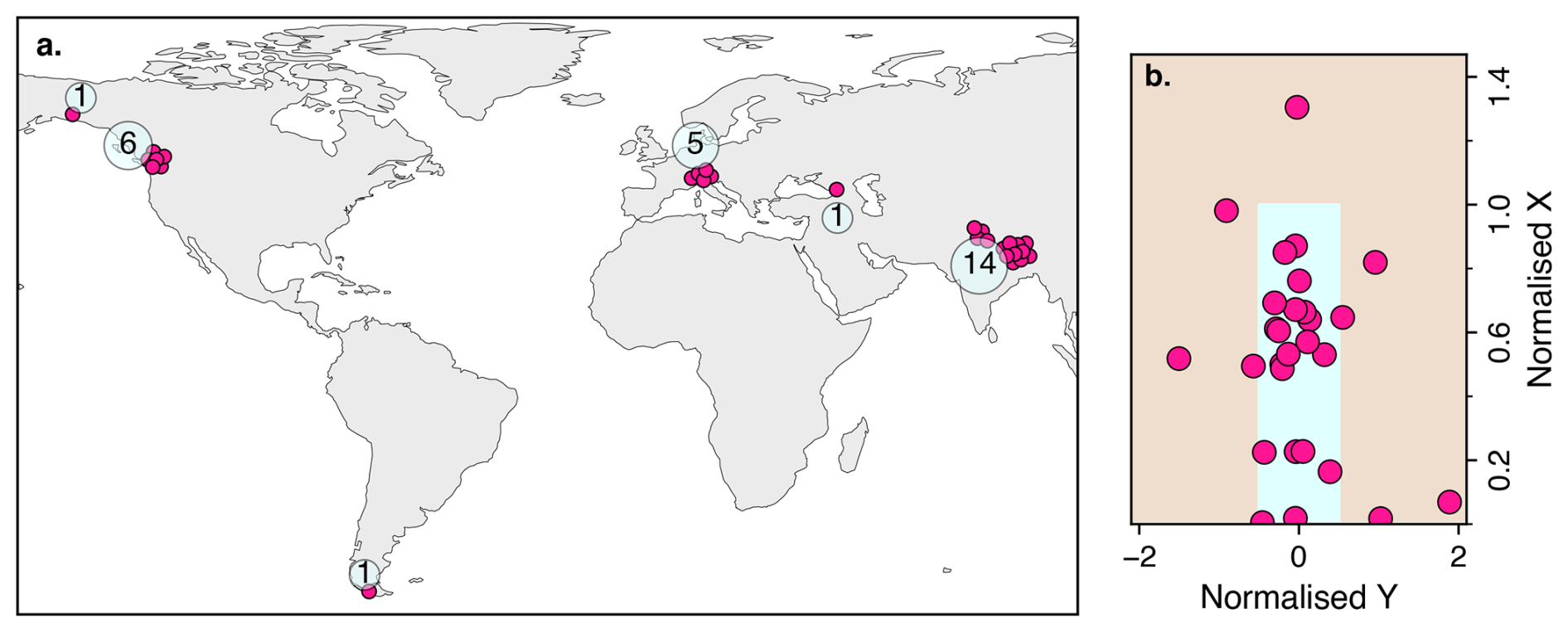
Figure 1 (a) Locations of 28 on- or near-glacier weather stations (red solid circles) used in this study. The circles have been artificially spread out up to about 2° to avoid overlap. The number of stations in different regions are shown within light blue circles. (b) The relative, scaled locations of the weather stations used in this study (red circles) with respect to an idealised glacier (light blue rectangle) having a unit length and width. Here X and Y denotes the longitudinal and transverse distance, respectively, with respect to a coordinate system whose origin is at the headwall of the idealised glacier, and X increases downglacier.

3 Methods

3.1 Model

3.1.1 Model for wind speed

Empirically, glacier wind is known to have a characteristic diurnal variation, with the maximum wind speed occurring in the afternoon (e.g., Obleitner, 1994; Oerlemans et al., 1999; Björnsson et al., 2005). It has also been noted that the timing of the wind speed maxima lags behind that of the temperature by a few hours (Oerlemans and Grisogono, 2002). The time series of the observed wind speed and ERA5-derived temperature for Drang Drung Glacier, the western Himalaya illustrate this behaviour (Fig. 2). It may be seen that the hourly wind speed signal is noisy (Fig. 2a). However, the mean diurnal wind speed has a relatively smooth variation, which appears to be a delayed response to the mean diurnal 2 m air temperature on this glacier (Fig. 2b). A similar behaviour is known to be present in valley-wind systems, and consequently, it could be described well using simple linear-response models (e.g., Nickus and Vergeiner, 1984). A similar linear-response model exists for land-sea breeze (Bjerknes, 1898).

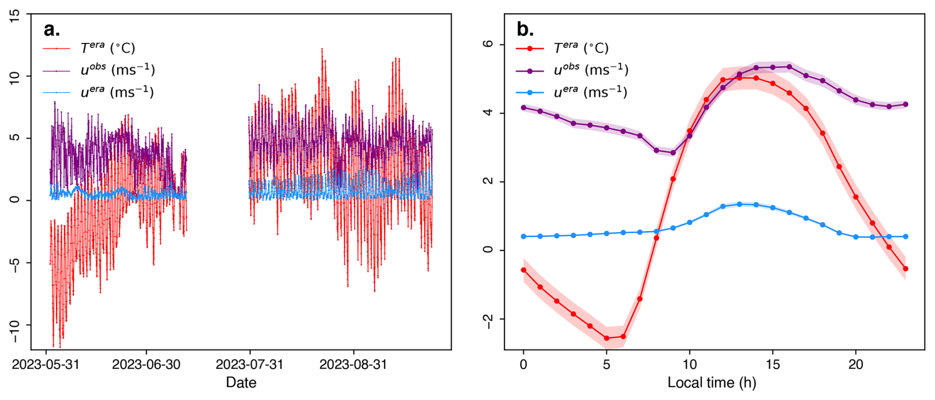
Figure 2 (a) Time-series of hourly wind speed (purple line) observed on Drang Drung Glacier in the western Himalaya, along with corresponding ERA5-Land temperature (red line) and wind speed (light blue line) estimates during the summer season of 2023. (b) The corresponding mean diurnal cycles, with the standard error of mean shown as shaded bands.

Motivated by this, here we attempted to predict the mean diurnal wind speed for both glacier winds and valley winds on or near a glacier, using the corresponding mean diurnal temperature. We restricted our analysis to the summer season as most of the melt happens during this time. We used a coordinate system in which z axis points vertically up and x axis is along the glacier flow direction. We assume that winds are generally either in the upslope or downslope direction. We decomposed the mean summertime diurnal wind speed u, into its mean value $\overline{u}$ and the diurnal anomaly u_d, i.e., $u\doteq \overline{u}+u_{\mathrm{d}}$. Similarly, the mean summertime diurnal temperature was decomposed into $\overline{T}$ and T_d. Then, we modelled u_d as an empirical linear combination T_d and its time derivative $\frac{d}{dt}{T}_d$, to obtain the following equation:

$$\begin{array}{}\text{(1)}& u=\overline{u}+s{T}_{\mathrm{d}}-s\mathit{\tau }{\displaystyle \frac{\mathrm{d}}{\mathrm{d}t}}{T}_{\mathrm{d}},\end{array}$$

where, s is the sensitivity of the mean diurnal wind speed anomaly to that of temperature, and τ is the corresponding time-scale parameter. Note that this is not a linear-response model (e.g., Boyce et al., 2017; Oerlemans, 2005), where the forcing variable (e.g., T_d) is taken to be an empirical linear combination of the response variable (e.g., u_d) and its time derivative. We chose the present empirical version over a traditional linear-response model because the derivative of wind speed was found to be relatively more noisy as compared to that of temperature (Fig. 2b), which resulted in poor fits. In our problem, the dominant frequency ω was diurnal (∼0.26 h⁻¹) and the typical time-scale parameter τ was ∼1 h, so that ω²τ²≪1. In this limit, both models were, in fact, equivalent to each other (Sect. S1 in the Supplement).

3.1.2 Extracting model parameters for the station

The model parameter $\overline{u}$ for each of the 28 stations was obtained by averaging the observed mean summertime diurnal wind speed u^obs. The remaining two model parameters s and τ were obtained for each station by performing a bilinear least-square regression of T_d and its derivative $\frac{\mathrm{d}}{\mathrm{d}t}{T}_{\mathrm{d}}$, against $u_{\mathrm{d}}^{\mathrm{obs}}$ (Eq. 1). This obtained 28 triplets of best-fit parameters {$\overline{u}$, s, τ} – one each for each station. Here, the diurnal variation T_d was obtained by decomposing the ERA5L-derived mean diurnal summertime temperature T, into its mean and the anomalies. The time derivative $\frac{\mathrm{d}}{\mathrm{d}t}{T}_{\mathrm{d}}$ at time step i was approximated as $\left(T_i-T_{i-\mathrm{1}}\right)/\mathrm{\Delta }t$, where T_i is temperature at ith time instant and Δt is the time step, which is 1 h.

3.1.3 Estimating model parameters for ungauged glaciers

To apply the above model to an ungauged glacier, one requires the knowledge of T_d and the three model parameters $\overline{u}$, s, and τ for that valley. It is possible to estimate T_d from reanalysis datasets. However, the model parameters are not known a priori. We derived predictors for each model parameter based on some simple dimensional arguments, expressing them in terms of easy-to-access variables like temperature and slope.

Let us denote the air density with ρ and acceleration due to gravity with g. Let the ambient air temperature (temperature at a same elevation as the glacier, but far away from the glacier) be denoted as T_a, and the air temperature near glacier surface be T_a+ΔT_a. Note that ΔT_a is positive for anabatic winds and negative for katabatic winds. Assuming the air temperature near a melting glacier surface is close to 273 K, the magnitude of ΔT_a may be approximated by the absolute value of the mean summertime ERA5-Land temperature expressed in degrees Celsius, denoted by $\left|\overline{T}\right|$. For steady slope winds, the buoyancy term B in the momentum equation is equal to turbulent friction term F (Oerlemans, 2010). The buoyancy term is given by:

$$\begin{array}{}\text{(2)}& B={\displaystyle \frac{g\left|\overline{T}\right|\sin \left(\mathit{\varsigma }\right)}{T_{\mathrm{a}}}}\end{array}$$

Here ς is the surface slope, and we have assumed sin ς≐ς for gentle slopes, which is true for most glaciers studied here. Since the ambient temperature across stations varies at most 10 % of its absolute magnitude (∼300 K), the B-term is likely to scale as follows:

$$\begin{array}{}\text{(3)}& B\sim \left|\overline{T}\right|\mathit{\varsigma }\end{array}$$

The turbulent friction term F in the momentum equation is estimated as ${\partial }_z\stackrel{\mathrm{‾}}{u^{\prime }{w}^{\prime }}$, where u^′ and w^′ are high frequency components of horizontal and vertical wind speeds (e.g., Oerlemans, 2010). We assume u^′ to scale as u, w^′ to scale as w, and denote the vertical scale of the winds by H. For winds flowing along the slope, the vertical component of wind velocity w is related to the horizontal component u, as w∼uς.

$$\begin{array}{}\text{(4)}& F={\partial }_z\stackrel{\mathrm{‾}}{u^{\prime }{w}^{\prime }}\sim {\displaystyle \frac{uw}{H}}\sim {\displaystyle \frac{u^{\mathrm{2}}\mathit{\varsigma }}{H}}\end{array}$$

From Eqs. (3) and (5), for steady slope wind,

$$\begin{array}{}\text{(5)}& {\displaystyle \frac{u^{\mathrm{2}}\cancel{\mathit{\varsigma }}}{H}}\sim & {\displaystyle }\left|\overline{T}\right|\cancel{\mathit{\varsigma }}.\text{(6)}& {\displaystyle }\Rightarrow u^{\mathrm{2}}\sim & {\displaystyle }H\left|\overline{T}\right|\end{array}$$

Steeper (gentler) glaciers are generally small (large), and therefore tend to have a smaller (larger) elevation range H. Assuning that H is related to elevation range, $H\sim H\mathit{\varsigma }/\mathit{\varsigma }\sim \mathrm{1}/\mathit{\varsigma }$. Therefore we propose that the variability in u is controlled by the ratio $\left|\overline{T}\right|/\mathit{\varsigma }$.

$$\begin{array}{}\text{(7)}& \Rightarrow u^{\mathrm{2}}\sim {\displaystyle \frac{\left|\overline{T}\right|}{\mathit{\varsigma }}}.\end{array}$$

The sensitivity of wind speed variation to temperature variation s is likely related to the ratio of the diurnal wind-speed range to the temperature range. Assuming that near the glacier surface, the diurnal wind speed range scales as the horizontal wind speed u, and that the diurnal temperature range scales as θ, we have:

$$\begin{array}{}\text{(8)}& s\sim {\displaystyle \frac{u}{\mathit{\theta }}}\sim {\displaystyle \frac{\mathrm{1}}{\sqrt{\left|\overline{T}\right|\mathit{\varsigma }}}}.\end{array}$$

The model parameter τ, which is the response-time scale, is assumed to scale with the ratio of some characteristic horizontal length scale (L) to the wind-speed scale (u). This leads to the following approximate relation:

$$\begin{array}{}\text{(9)}& \mathit{\tau }\sim {\displaystyle \frac{L}{u}}\sim \mathit{Ł}\sqrt{{\displaystyle \frac{\mathit{\varsigma }}{\left|\overline{T}\right|}}}.\end{array}$$

We search for a good candidate for ς by trial and error from among various possible choices. These include the glacier slope, and three versions of topographic slope computed at scales of 0.1, 1, and 10 km (Table S2). We also consider all possible ratios of seven vertical (e.g., glacier elevation range, relief, etc.) and three horizontal length scales (e.g., length of glacier, width of glacier, etc.). In total, we tested 25 possible candidates for the RHS of Eqs. (7)–(9). Given the limited sample size of only 28 stations and the generally high noise level, we relied primarily on visual comparison to assess the performance of these candidates. The 28 model parameter triplets were plotted against their corresponding predictor values and visually assessed for linear relations of the form:

$$\begin{array}{}\text{(10)}& {\displaystyle }\overline{u}& {\displaystyle }={\mathit{\beta }}_{\mathrm{1}}\sqrt{{\displaystyle \frac{\left|\overline{T}\right|}{\mathit{\varsigma }}}},\text{(11)}& {\displaystyle }s& {\displaystyle }={\mathit{\beta }}_{\mathrm{2}}{\displaystyle \frac{\mathrm{1}}{\sqrt{\left|\overline{T}\right|\mathit{\varsigma }}}},\text{(12)}& {\displaystyle }\mathit{\tau }& {\displaystyle }={\mathit{\beta }}_{\mathrm{3}}\mathit{Ł}\sqrt{{\displaystyle \frac{\mathit{\varsigma }}{\left|\overline{T}\right|}}},\end{array}$$

where β₁,β₂, and β₃ are the best-fit regression coefficients. If no clear relationship was seen between a model parameter and any of its predictors, the median value of that model parameter across the 28 stations was used as the predictor.

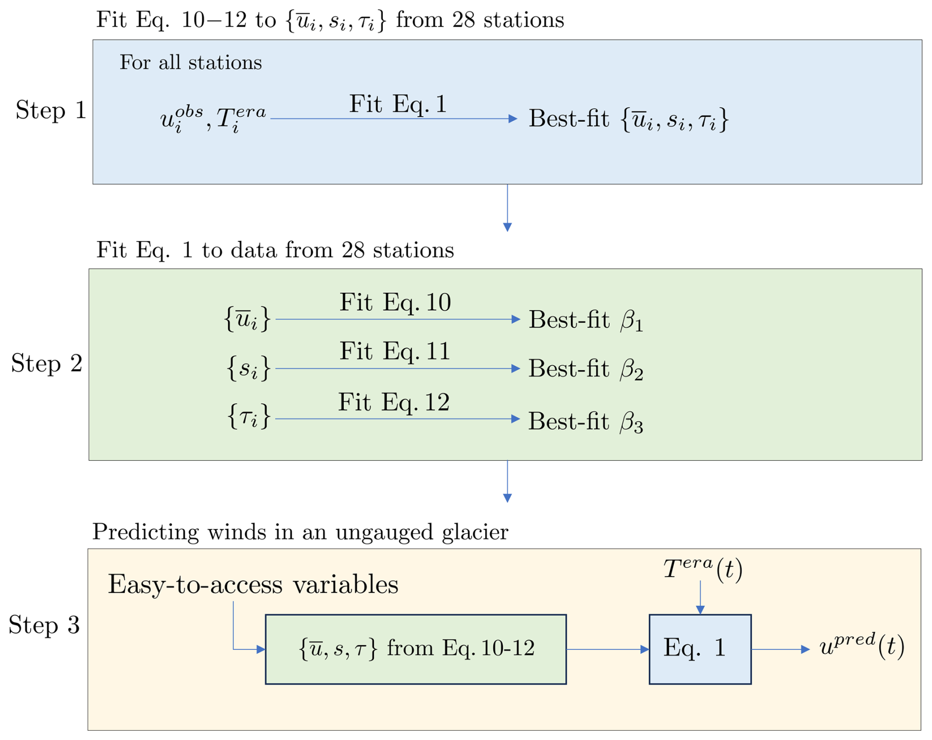
Figure 3 The workflow for modelling the mean summertime diurnal wind on an ungauged glacier employed in this paper. Step 1: Observed wind speed and ERA5 temperature at each station were fitted to Eq. (1) separately, obtaining 28 triplets of best-fit $\mathit{\{}\overline{u},s,$ and τ}. Step 2: This set of 28 triplets were used to obtain the best-fit regression coefficients defined in Eqs. (10)–(12). Step 3: For any ungauged glacier location, the best-fit Eqs. (10)–(12) were used to predict the three model parameters, which along with the corresponding ERA5L temperature, were fed to Eq. (1) to obtain the wind speed predictions.

3.2 Model performance

3.2.1 Performance of the calibrated model

The performance of the calibrated model (Eqs. 1, 10–12), was assessed on each of the 28 weather stations. For each station, the mean summertime diurnal wind speed predicted by the calibrated model at hourly time steps were compared with the corresponding observed values. The mean, median, and interquartile range of the set of 28 root-mean-squared errors (RMSE) between the model predictions and observations were compared with the set of RMSEs between the ERA5L products and observations. Note that these predicted u values were obtained from the calibrated equations, only using the corresponding ERA5L temperature and the static variables as inputs.

3.2.2 Leave-One-Out-Cross-Validation

To evaluate the performance of the model for an ungauged location, we performed a Leave-One-Out-Cross-Validation (LOOCV) (Hastie et al., 2009). For this, we calibrated the model following the procedure described in Sect. 3.1.2 and 3.1.3 with 27 out of 28 weather stations. We find out the best-fit values of β₁,β₂ and β₃ in each iteration and use them to predict the model parameters. The calibrated model was then used to predict the wind speed at the left-out 28th weather station, using only the corresponding ERA5L temperature and slope, and without using any in-situ data from the left-out station. We repeated this process 28 times, leaving out a different station each time, and computing the RMSE between the predicted and observed wind speeds for the left-out station. The mean, median, and interquartile range of the set of 28 RMSEs thus obtained were compared with the set of RMSEs between the ERA5L products and observations. We do not consider the uncertainties in the predicted model parameters in this LOOCV analysis. Also, we assume the same form of Eqs. (10)–(12) in each iteration, without repeating the search for the best set of choices for the temperature and slope variables. The present estimates of model performance in this LOOCV protocol are likely to be conservative, as we may not be working with the best model in some of the iterations.

3.2.3 Minimum number of stations required

We tested how sensitive the predictions from the calibrated model were to the number of stations available for calibration. To do this, the model was calibrated only using a randomly selected subset of N stations. For each subset, the model was calibrated exactly as discussed in Sect. 3.1.2–3.1.3, and then evaluated across all 28 stations by computing the RMSEs between the observed and predicted mean summertime diurnal wind speed. The median RMSE was recorded. The step was repeated for $N=\mathrm{13},\mathrm{14},\mathrm{\dots },\mathrm{28}$. The exercise was repeated 100 times to obtain a set of 100 mean RMSEs for each N. The resulting distributions of RMSEs were plotted as a function of N, to see if the RMSEs converge to a fixed value with increasing N. The minimum value of N, for which the median RMSE differed by less than 1 % from that obtained for N=28, was defined as the minimum number of stations required for model calibration. Note that this exercise was also helpful in ascertaining the model performance on ungauged glaciers, as only a subset of glaciers were used here to calibrate the model, which was then used to predict the wind speed on all 28 stations.

3.3 Estimation of uncertainty

The uncertainty in the predicted windspeed was estimated via a Monte-Carlo simulation with 1000 iterations. In each iteration, the triplet of model parameters were drawn from a corresponding Gaussian distribution. The mean of the Gaussian represented the best model listed later in Eqs. (13)–(15). The standard deviations of the Gaussian distributions were chosen either from the fit errors of the linear regressions (Eqs. 10–12) or from the IQR of the empirical distribution of the corresponding parameter, as applicable (see Sects. 3.1.3 and 4.1.2). A Gaussian noise was also added to the input values of T^era, which had zero mean and the standard deviation was equal to the standard error of mean (Fig. 2b).

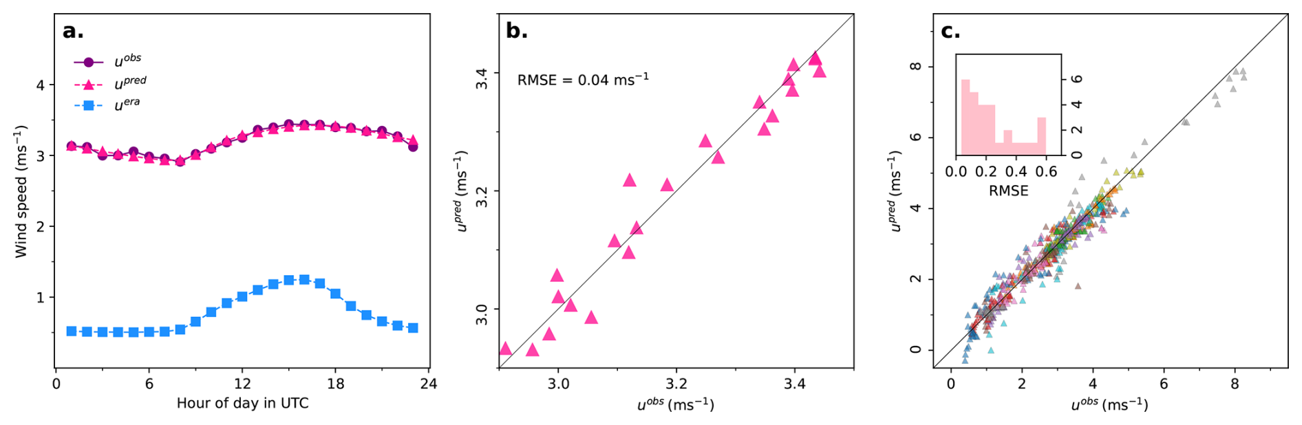
Figure 4 (a) Predicted mean summertime diurnal wind speed (red solid triangle) obtained by fitting Eq. (1) to the observed wind speed (purple solid circle) and ERA5L temperature for a selected weather station (Place Glacier in British Columbia, see Table S1). (b) Comparison of the predicted and observed mean wind speeds for this station. (c) Comparison of the predicted and observed mean wind speed for all 28 station, with different symbol colours denoting different stations. The inset shows the distribution of RMSEs obtained in the fits.

4 Results

4.1 Model calibration

4.1.1 Extracting model parameters for the stations

The linear-response equation (Eq. 1) reasonably captured the mean summertime diurnal wind speed across all the weather stations. The results of fitting Eq. (1) to the observed wind speed and ERA5L temperature on a selected weather station shown in Fig. 4. Across the 28 weather stations, the quality of fits varied (Fig. 4c). The mean (median) RMSE was 0.24 (0.17) m s⁻¹, and an interquartile range of 0.12–0.36 m s⁻¹ (Table S3). In contrast, a direct comparison between the ERA5L wind-speed product with the observed mean summertime diurnal wind yielded a mean (median) RMSE of 1.99 (2.11) m s⁻¹, with an interquartile range of 1.31–2.57 m s⁻¹.

The distribution of best-fit model parameter triplet $\mathit{\{}\overline{u},s,$ and τ} obtained for the 28 stations showed a significant variability between stations (Fig. S2). The best-fit mean wind speed $\overline{u}$ ranged from 0.96–5.12 m s⁻¹ with a mean (median) value of 2.71 (2.96) m s⁻¹. The best-fit sensitivity s ranged from 0.0–1.04 m s⁻¹ °C⁻¹ with a mean (median) value of 0.27 (0.18) m s⁻¹ °C⁻¹. The best-fit time-scale parameter τ ranged between 0–3.4 h, with a mean (median) value of 1.07 (0.68) h.

4.1.2 Estimating model parameters for ungauged glaciers

The predictor $\sqrt{\left|\overline{T}\right|/{\mathit{\varsigma }}_{\mathrm{10}}}$ was found to be the most suitable to estimate model parameter $\overline{u}$ (Fig. 5a), where $\left|\overline{T}\right|$ is the absolute value of the mean summertime temperature $\overline{T}$ from ERA5L (Sect. 2.2), and ς₁₀ is the topographic slope of the station for a resampled 10 km resolution DEM using a 3×3 window. A regression between this predictor and the observed best-fit values of $\overline{u}$ yielded an R² value of 0.9 (p<0.001), confirming a strong relationship. The next best model was $\sqrt{\left|\overline{T}\right|/{\mathit{\varsigma }}_g}$, where ς_g is the mean glacier slope, which had an R² value of 0.83 but was not significant within p<0.01 level (Fig. S3). For the case of model parameter s, no reliable predictor could be found (Sect. S2). The predictor $\mathrm{1}/\sqrt{\left|\overline{T}\right|/{\mathit{\varsigma }}_{\mathrm{10}}}$ had the highest R² of 0.57 (p<0.001). However, visual inspection indicated that this apparent performance was likely influenced by an outlier (Fig. 5b). After excluding the outlier, the R² value decreased to 0.32, which was not significant at the p<0.01 level. Therefore, we used the median value of s across the 28 stations as its predictor. For the model parameter τ, none of the candidate predictors performed well on visual inspection (Fig. 5c). The best-performing predictor, $L_{\mathrm{g}}\sqrt{{\mathit{\varsigma }}_{\mathrm{10}}/\left|\overline{T}\right|}$, where L_g is glacier length, was not significant, confirming the absence of a strong relationship. We therefore obtained the following parameterisations:

$$\begin{array}{}\text{(13)}& {\displaystyle }\overline{u}& {\displaystyle }=(\mathrm{0.268}\pm \mathrm{0.017})\sqrt{{\displaystyle \frac{\left|\overline{T}\right|}{{\mathit{\varsigma }}_{\mathrm{10}}}}},\text{(14)}& {\displaystyle }s& {\displaystyle }=\mathrm{0.18}\pm \mathrm{0.25},\text{(15)}& {\displaystyle }\mathit{\tau }& {\displaystyle }=\mathrm{0.7}\pm \mathrm{1.4}.\end{array}$$

In the above three equations the uncertainty is the standard error of regression in Eq. (13). Whereas, for Eqs. (14)–(15), it is the standard deviation of the Gaussian distribution with the same inter-quartile range as the “observed” distributions of corresponding set of 28 corresponding observed best-fit model parameters as described in Sect. 3.1.2.

The mean wind speed ${\overline{u}}^{\mathrm{pred}}$ predicted using Eq. (13) compared favourably with the corresponding observed values, with a mean RMSE of 0.57 m s⁻¹ (Fig. 5a). In comparison, the corresponding mean RMSE for the ERA5L product was 1.87 m s⁻¹, which was 3.3 times higher. The diurnal wind speed anomaly $u_{\mathrm{d}}^{\mathrm{pred}}$ predicted using Eqs. (1), (14)–(15), matched the observations $u_{\mathrm{d}}^{\mathrm{obs}}$ reasonably well with an mean RMSE of 0.49 m s⁻¹. In comparison, ERA5L predicted the diurnal anomaly with an mean RMSE of 0.46 m s⁻¹, which was comparable to our model.

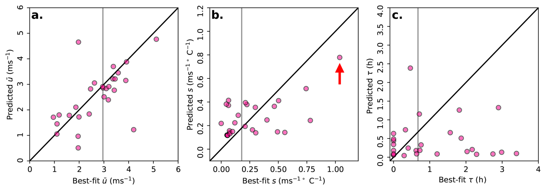
Figure 5 The value of model parameters predicted by Eqs. (10)–(12) are plotted against their observed best-fit values from all 28 stations. The grey vertical line shows the median value of each model parameter across all stations. (a) The predictor $\sqrt{\frac{\left|\overline{T}\right|}{{\mathit{\varsigma }}_{\mathrm{10}}}}$ was found to have a strong relationship with $\overline{u}$, with an R² of 0.9 (p<0.001). (b) For s, the predictor $\mathrm{1}/\sqrt{\left|\overline{T}\right|/{\mathit{\varsigma }}_{\mathrm{10}}}$ was found to have a significant relationship with an R² of 0.57 (p<0.001), but upon removal of the data point marked with red arrow, the relationship became insignificant. (c) None of the predictors discussed in Sect. 3.1.3 showed a significant relation with τ. Due to the lack of predictability of s and tau, we used the corresponding median values to estimate them for ungauged glaciers, which does not capture variability of these quantities between glaciers.

4.2 Model performance

4.2.1 Performance of calibrated model

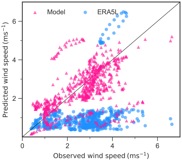
The calibrated model (Eqs. 1, 13–15) was able to capture the mean summertime diurnal wind speed better than the corresponding ERA5L product for all the weather stations (Fig. 6). For example, the RMSE of the predicted wind speed had a mean (median) value of 0.87 (0.64) m s⁻¹, and an interquartile range of 0.42–0.88 m s⁻¹. In comparison, the ERA5L wind speed product had two times higher mean of 1.98 m s⁻¹, three times higher median of 2.09 m s⁻¹, and a two times larger interquartile range of 1.29–2.57 m s⁻¹ (Table S3).

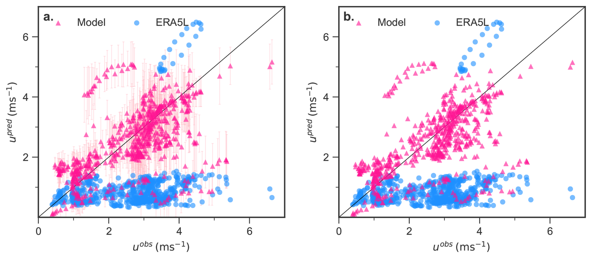
Figure 6 The mean summertime diurnal wind speed predicted using Eqs. (1), (10)–(12) (red solid triangle) were compared with corresponding observation. The corresponding comparison for ERA5L wind speed are also shown (blue solid circles). (b) The result of LOOCV (main text, Sect. 4.2.2): For each of the 28 left-out stations, the predicted u is compared to the corresponding observed values. The ERA5L wind speeds for the left-out stations are also shown (blue solid circles).

4.2.2 Leave-One-Out-Cross-Validation

In general, the result of the LOOCV was satisfactory, and the model fitted to data from 27 stations was able to predict the mean diurnal wind speed at the left-out station reasonably well (Fig. 6b and Table S3). In comparison to ERA5L, the set of 28 RMSEs of the wind speed predicted for the left-out station by the corresponding calibrated model had two times lower mean (0.87 m s⁻¹), three times lower median (0.64 m s⁻¹), and three times lower interquartile range (0.42–0.88 m s⁻¹). We do not find any clear pattern in the spatial distribution of the RMSE values (Fig. S8).

4.2.3 Minimum number of stations

A general decline in model performance with decreasing N was observed. The mean RMSE for the predictions over all 28 stations was 0.853 m s⁻¹ for N=21, which was within 1 % of the mean RMSE value of 0.848 m s⁻¹ obtained when all N=28 stations were used for calibration. This indicates that as long as the number of weather stations available for calibration N was 21 or more, the calibrated model was reliable (Fig. 7a).

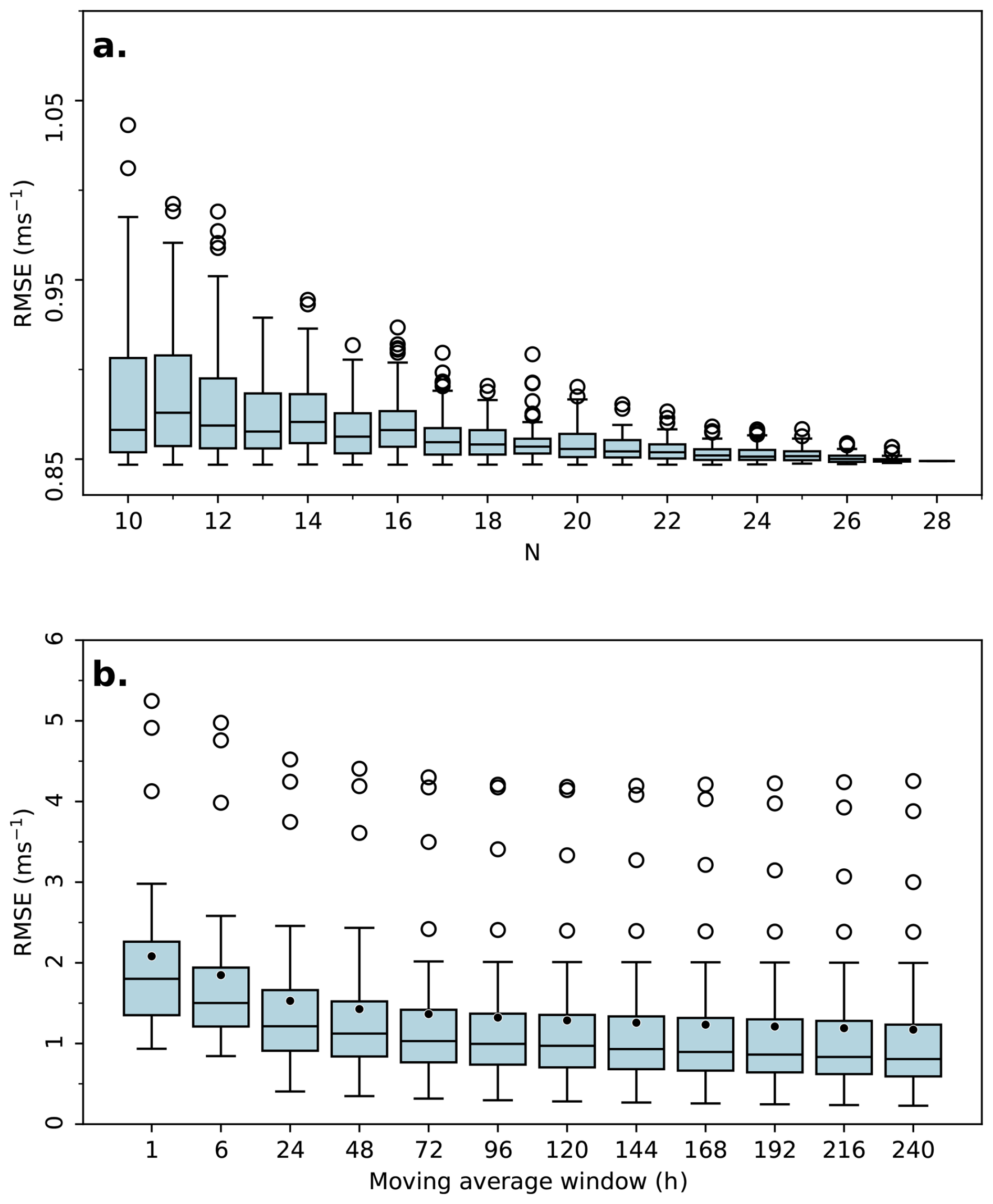
Figure 7 The distribution of RMSEs between predicted and observed wind speed for (a) different number of stations N used to calibrate the model, and (b) different time-averaging windows. The mean (solid black circle), median (horizontal black line), and outliers (open black circles) of the distributions are shown.

5 Discussion

5.1 Predicting wind speed on ungauged glacier

The proposed model for the mean summertime diurnal wind speed (Eq. 1), which computed the local wind speed on/around glaciers with ERA5L temperature as input, worked reasonably well for all the 28 weather stations. This may not be unexpected given the existing studies, where thermally driven wind systems such as land-sea breezes and valley-wind circulation have been successfully described as a linear response to diurnal pressure-gradient forcing (e.g., Nickus and Vergeiner, 1984; Vergeiner and Dreiseitl, 1987; Bjerknes, 1898).

The novel result in this study is that the three associated triplet of model parameters $\mathit{\{}\overline{u},s,$ and τ} could be predicted for any given glacier using the relations Eqs. (13)–(15), without the need for any in-situ data. It is apparent from the LOOCV analysis (Sect. 4.2.2) and the performance of the models calibrated with a smaller subset of stations (Sect. 4.2.3), that the performance of the present model on ungauged glaciers, is quite robust. The present model, thus, appears to be a reliable and parsimonious alternative to the presently available methods and products, for estimating local wind speed on ungauged glaciers.

Interestingly, the model appears to perform quite well also for the 13 stations that are located near a glacier, and not on it (Fig. S4). In addition, it works well for five stations located on debris-covered glaciers (Fig. S1). In all these 16 cases, the station locations are dominated by valley winds, and not by glacier winds. This suggests that both valley and glacier winds are captured by the same model to a good approximation.

5.2 Predictability of model parameters

The strength of the present model, which predicts the mean summertime diurnal wind speed on any glacier with only ERA5L temperature as input, is that the model parameter $\overline{u}$ can be calculated from mean temperature and regional slope (Eqs. 13). However, the predictability of the other two model parameters s and τ was relatively low (Fig. 5b, c). In fact, most of the improvements in wind speed predicted by the present model, over that obtained from ERA5L, was due to the ability of the present model to capture the variability of the mean wind speed $\overline{u}$ between stations (Sect. 4.1.2). Perhaps with more data, a larger set of stations, having a higher time resolution, can help improving the predictability of the remaining parameters.

Time-scales of prediction

We tested if the calibrated model, which was derived for mean summertime diurnal winds, could be used to predict wind speeds across different time-scales. We first filtered the ERA5L hourly temperature data over different time-scales by taking 1 h to 10 d moving average. For each station and each averaging window, the filtered temperature data were fed into the calibrated model (Eqs. 1, 13–15) to obtain wind speed predictions for that station and that time-scale. While the calibrated model performed better than ERA5L wind speed product across all time-scales, its performance reduced at finer time-resolutions (Fig. 7b). For moving-average windows of length greater than 96 h, the distribution of RMSEs between observed and predicted winds across the 28 stations had a median value below 1 m s⁻¹. For shorter time-averaging lengths, the median RMSE increased systemically, with RMSE of ∼1.8 m s⁻¹ for hourly predictions. In comparison, the ERA5L wind speed product had a median RMSE of more than 2 m s⁻¹ across all the time-averaging lengths. It appears that model, which is calibrated for the mean diurnal wind speed over the entire summer season, is still useful at shorter times scales as well. This maybe because the variability of the mean diurnal wind speed averaged over several days is less than that of the mean wind speed between glaciers (Fig. 5b), which the model is able to capture. An analysis of variance of observed and predicted wind speed data across different time-scales (Fig. S5) revealed that this improvement in prediction is not simply due to a reduction in variance due to higher smoothing.

5.3 Implication for melt calculations

For a rough estimate of the effects of improved estimates of surface wind speed on ice melt calculations, we used a simple bulk-aerodynamic formulation (e.g., Cuffey and Paterson, 2010) to compute the hourly sensible (Q_shf) and latent (Q_lhf) heat fluxes for the entire data range of all the 28 stations as follows:

$$\begin{array}{}\text{(16)}& {\displaystyle }{Q}_{\mathrm{shf}}& {\displaystyle }=\mathrm{0.0129}{C}^{*}PuT,\text{(17)}& {\displaystyle }{Q}_{\mathrm{lhf}}& {\displaystyle }=\mathrm{22.2}{C}^{*}u(e-e_{\mathrm{s}}).\end{array}$$

Here, $C^{*}=\mathrm{0.002}$ is a transfer coefficient (Cuffey and Paterson, 2010), P is the air pressure (in Pa), T is the air temperature (in °C), e is the vapour pressure (in Pa) above the melting surface, and e_s is the vapour pressure (in Pa) at the melting ice surface. The variables P and T were obtained from ERA5. The saturation vapour pressure e_s and actual vapour pressure e were derived from the dew-point temperature obtained from ERA5L (Bolton, 1980). The sum of Q_shf and Q_lhf gave the total turbulent heat flux Q_thf. At each station, the turbulent heat flux calculations were repeated thrice for the different estimates of the mean wind speed $\overline{u}$, namely, (a) the observed ones, (b) those predicted using Eq. (13), and (c) those obtained directly from ERA5L.

The mean RMSE between the heat fluxes calculated using the observed wind speed (${\overline{u}}^{\mathrm{obs}}$) and that predicted using Eq. (13) (${\overline{u}}^{\mathrm{pred}}$) for all stations was 3.5 W m⁻² (Fig. 8), which was about three times smaller than the mean RMSE of 10.15 W m⁻² obtained for the ERA5L derived mean wind speed (${\overline{u}}^{\mathrm{era}}$). For 17 out of the total 28 stations, where the net Q_thf was positive, the heat fluxes increased by a factor of 3.7 on average (Table S4). For the remaining 11 stations with net negative turbulent heat fluxes, the magnitude of the fluxes increased by a factor of 2.3. This suggested that the turbulent heat fluxes on glaciers might be systematically underestimated when ERA5L wind-speed products are used. This is due to the general underestimation of surface-wind speed by ERA5L at the stations (Fig. 6). While Eq. (13) captures the variability of wind speed between stations, that does not necessarily ensure the corresponding estimates $Q_{\mathrm{thf}}^{\mathrm{pred}}$ reproduce well the variability of the total turbulent heat fluxes between the stations at a global scale. This is because the temperature and humidity dependent factors in Eqs. (16) and (17) can potentially vary strongly between regions. However, for a given region, the spatial variability of turbulent heat flux is likely to be controlled mainly by that of the wind speed. Therefore, the present model can help in improving the turbulent heat flux calculations for a region, compared to that derived from ERA5L wind speed. This is also seen from the three times lower mean RMSE between heat fluxes calculated using the model and that using ERA5L-derived winds. We emphasise that the values of turbulent heat fluxes estimated using the bulk aerodynamic method are meant to be illustrative in nature. Although such methods have been used widely and shown to outperform profile-based methods when a wind speed maximum is present (Denby and Greuell, 2000), some recent reports suggest they may perform poorly on glaciers where their underlying physical assumptions may be unrealistic (Litt et al., 2015; Radić et al., 2017; Steiner et al., 2018).

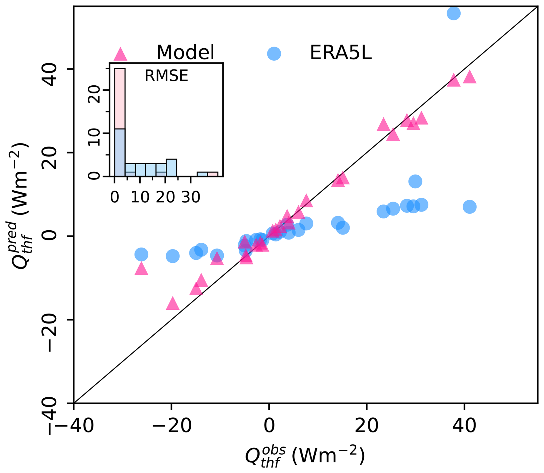
Figure 8 Total turbulent heat flux $Q_{\mathrm{thf}}^{\mathrm{pred}}$ derived using the mean wind speed predicted in this study (red triangles), and those from ERA5L (blue circles) are compared with the turbulent heat flux $Q_{\mathrm{thf}}^{\mathrm{obs}}$ computed using observed wind speed. Inset shows the corresponding distributions of RMSEs for the 28 stations.

5.4 Applicability of our model

It is important to assess whether the glaciers used in this study are representative of the global glacier population. If not, applying the model to ungauged glaciers may introduce extrapolation errors. The distributions of static glacier variables in our dataset were therefore compared with the global distributions from RGI7 (Fig. 9). Based on this comparison, the model is likely to work better for glaciers with:

1. Mean summertime temperature between −17 to 10 °C,

2. Mean summertime diurnal temperature range between 3 to 10 °C,

3. Mean glacier slope <0.6,

4. Glacier area >1 km²,

5. Glacier length >2 km,

6. Mean elevation >2000 m.

Our station distribution is biased toward larger and more gently sloping glaciers, which are generally easier to access. More than 80 % of the world's glaciers are smaller than 1 km², yet our dataset does not contain a single weather station from glaciers in this size range. Arguably, because such glaciers are typically located near mountain ridges, synoptic wind systems may dominate there rather than thermally driven flows. Also, the small, steep glaciers may not have well developed glacier wind (Sauter et al., 2026). In contrast, high-altitude glaciers in High Mountain Asia, despite being among the most challenging environments to access, are well represented in our dataset.

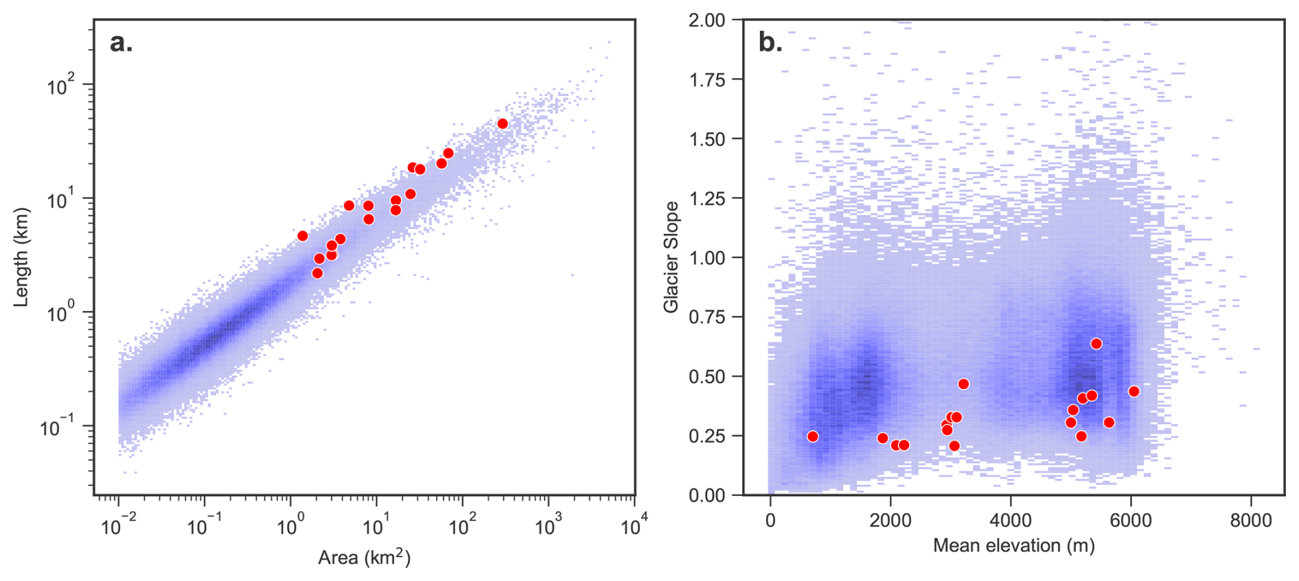
Figure 9 (a) The distribution of glacier length and glacier area for glaciers in this study (red dots) compared with that of the global population of glaciers (blue dots). Similar comparison for mean glacier elevation and glacier slope is shown in (b). Glaciers with a mean slope greater than 2 (22 glaciers) were excluded from panel (b) for clarity. Our stations are biased towards larger and gently sloping glaciers, suggesting the possibility of extrapolation errors for smaller steep glaciers.

5.5 Limitations

Ideally, a first-principle derivation for our Eq. (1) is required. We were unable to derive our model systematically from existing theories like the Prandtl model (Oerlemans, 2010). However, in general, it is difficult to derive linear-response relations for complex problems. We acknowledge that the present model provides only a first-order solution to the problem of estimating the surface winds on or near a glacier. The present results pertain to the mean summertime diurnal wind, while the wind speed is expected to vary over different timescales – hourly, daily,and weekly, (e.g., Fig. 2a) to seasonal and annual. However, our analysis over different time windows (Sect. 5.2.1) suggests that the magnitude of such temporal variability over time-scales of weeks or longer is often not very large compared to the variability of the mean winds between stations.

An inter-annual variation of the mean summertime wind speed was apparent at the stations with more than one year of data (Fig. S6). Such a temporal variability is, of course, not captured by the present model, which produces a time-independent prediction for mean winds at each station based on Eq. (13). For example, the mean value of the fractional absolute inter-annual deviation was less than 10 % in all but two of the studied locations (Fig. S6), suggesting that the mean wind speed predicted using Eq. (13) are still useful. More work is needed, possibly utilising a larger set of stations with longer records, and higher time resolution to see if the observed temporal variability could be incorporated into the present model with the help of additional time-dependent meteorological variables.

A significant spatial variability of the surface wind within any given glacierised valley is expected (e.g., Cai et al., 2007), which we do not try to capture with this present model. Only few studies report on within-glacier variation of wind speed and they differ in their conclusion (e.g., Strasser et al., 2004; Greuell et al., 1997; Zou et al., 2008). No clear spatial pattern for winds within the same valley was present in our dataset (Fig. S7). It should be noted, however, that only four out of 18 glaciers in our study had more than one station in the same valley. Hence, we do not attempt to explain within-glacier variation with our model and rather focus on between-glacier variability. Also, in glacierised valleys, there is a competition between the valley and the glacier winds at the surface level, which flow in opposite directions during the daytime. The present formulation is likely to fail over the region near the glacier terminus where these two winds collide. In fact, the present model gives only wind speed and not the wind direction.

There were some peculiarities in the mean summertime diurnal wind speed at a few stations, which could not be captured by the present model. For example, some stations there were additional early-morning maxima of wind speed (Fig. S1), apart from the prominent late-afternoon one. This behaviour could not be reproduced with the present temperature-based linear response model, as the mean diurnal temperature decreased monotonically between sunset and sunrise. At Langenferner Glacier, the temperature and wind speed was out of phase (Fig. S1), which was unusual. Here Eq. (1) could not be fitted to the data for a finite τ, and the wind speed predictions using Eqs. (1), (10)–(12) produced a large RMSE (Table S3).

Most of the improvement in mean summertime diurnal wind speed predicted using the present model, vis-a-vis the estimates obtained directly from ERA5L, was due to a better estimation of the mean wind speed ${\overline{u}}^{\mathrm{pred}}$ by the former. As discussed above, the mean RMSEs for ${\overline{u}}^{\mathrm{pred}}$ was three times smaller in the present model, compared to that of the corresponding ERA5L product. In addition, the ERA5L had a significant negative bias, which was 1.9 m s⁻¹ on average, for $\overline{u}$. Here we acknowledge that the ERA5L-derived 10 m wind speed is not directly comparable to the 2 m values. However, as discussed before, the interpolation of the value to 2 m level is complex. In contrast, both the present model and ERA5L had similar mean RMSEs for the diurnal anomaly u_d, indicating that there is scope for improving the estimates of the model parameters s and τ. As can be seen from the Fig. S2, 64 % of the stations have a τ less than the time resolution of our data (1 h). This might explain why it is difficult to parameterise the variability of τ.

6 Conclusion

In this study, we propose a model to estimate the mean summertime diurnal wind speed on any ungauged glacier. Given the values of three model parameters, the model obtains the wind speed as a linear combination of the mean summertime diurnal temperature and its time derivative. The required input temperature data are derived from a reanalysis product (ERA5-Land). Among the three model parameters, the parameter $\overline{u}$, which is the mean summertime wind speed, can be estimated from mean reanalysis temperature and regional slope. For the sensitivity parameter s and time-scale parameter τ, we prescribe to use the median values obtained from the corresponding “observed” values from 28 weather stations. We show that this model captures well the observed mean summertime diurnal wind speed on 28 on- or near-glacier weather stations across the globe. Interestingly, an analysis of 28 weather stations established that mean wind speed parameter $\overline{u}$ can be estimated using simple linear functions of temperature and slope. This implies that the present model can be applied to ungauged glaciers, which is encouraging. A leave-one-out-cross-validation indicated that the method indeed works reasonably on ungauged glaciers, and may improve the RMSE between the observed and estimated mean summertime diurnal wind speeds by about 200 % on average, compared to the corresponding reanalysis estimates. Most of this improvement is, in fact, due to the ability of the present model to capture the variability of the mean summertime wind between glaciers better than the reanalysis product. The number of stations used for calibrating the model is shown to be adequate for robust predictions. We discuss the limitations of the model in capturing the temporal variability of wind speed over different time-scales. Although winds are expected to have a within-glacier spatial variability, due to the limited sample size and noise in the data, we could not robustly assess this in our model. Using this model to parametrise the mean summertime diurnal wind speed may improve the turbulent heat flux estimates on glacierised valleys, which tend to be underestimated with reanalysis wind speed products. Improving the estimates of the other two model parameters, and developing a similar model for smaller timescales, and finding the physical mechanism that explains the success of the empirical model emerge the three most interesting open problems.