Sensitivity of Andean Glaciers to ice-flow parameters in the Parallel Ice Sheet Model

Mountain glaciers are losing mass rapidly due to anthropogenic climate change. Projections of glacier evolution across the Andes under different warming scenarios have primarily been as part of global scale modelling frameworks, rather than dedicated, regionally optimised, simulations. These global-scale models use simplifications of ice flow physics that may be unsuitable for steep topography, such as that which occurs at mountain valley glaciers. More complex models are available, but with that complexity comes further sources of uncertainty. Here, we assess the sensitivity of the Parallel Ice Sheet Model to ice-flow parameters influencing the ice rheology and subglacial sliding characteristics. We find that the resistance of subglacial material has the most impact on modelled ice outputs (e.g., ice volume), followed by the exponent which relates basal shear stress to sliding, and the threshold velocity at which sliding occurs. The ice-flow rheology enhancement factors, the rate of subglacial water decay, and the maximum water thickness within a presumed subglacial drainage network, can either cause minor variations, or no effect at all, on ice outputs in our model configuration. Our study informs what parameters can potentially be negated in future parameter ensemble tests and provides direction on where further investigation is needed.

1 Introduction

Andean glaciers are a critical part of the region's water tower system (Immerzeel et al., 2020), particularly during droughts (Drenkhan et al., 2015) and in upland rural areas (Buytaert et al., 2017; Rabatel et al., 2013). However, they are losing mass rapidly (Dussaillant et al., 2019), placing stress on water resources, and contributing to sea level rise. Continued global warming, intensified by regional elevation-dependent warming (Byrne et al., 2024; Pepin et al., 2015), and changing precipitation regimes (Cai et al., 2020; Masiokas et al., 2020; Potter et al., 2023) heighten the need for accurate glacier projections to inform water management and sea level rise assessments.

Global-scale models of glaciers and ice caps (i.e., all land-based ice not stored in ice sheets) predict continued ice loss through to 2100 (Hock et al., 2019; Hugonnet et al., 2021; Rounce et al., 2020). While long-term sea level rise will be dominated by the Greenland and Antarctic Ice Sheets (Goelzer et al., 2020; Seroussi et al., 2024), glaciers and ice caps may contribute up to 0.35 m of sea level rise by 2100 (Edwards et al., 2021; Hock et al., 2019; Marzeion et al., 2020). These global-scale experiments are designed to capture the envelope of plausible sea level rise contributions from glaciers under different emission scenarios (Fox-Kemper et al., 2023). However, global and regional scale projections of mountain glacier change are not only needed for sea level rise, but also for management of changing water resources, mountain glacier hazards, resources for tourism and recreation, and for ecological and biodiversity management.

Glacier models used in intercomparison efforts such as GlacierMIP (Hock et al., 2019; Marzeion et al., 2020; Rounce et al., 2023) provide insight at global and regional scales (Zekollari et al., 2025). However, their use may be limited for planning local resource management and mitigations due to: (i) simplified ice-flow physics unsuited to steep topography (Egholm et al., 2011); (ii) reliance on downscaled global climate models (GCMs), which often poorly capture mountain climate (Núñez Mejía et al., 2023); and (iii) simplified mass balance schemes, often reduced to positive degree-day models (PDD; Bolibar et al., 2022).

Here we attempt to address the first issue, by using a complex ice sheet model to assess uncertainties in the parameterisation of glacier ice flow physics in areas of steep mountain topography. We use the Parallel Ice Sheet Model (PISM; Winkelmann et al., 2011), a thermomechanically coupled shallow-ice/shallow-shelf model commonly applied to both ice sheets (Johnson et al., 2023; Payne et al., 2021; Seroussi et al., 2024) and mountain glaciers (e.g., Candaş et al., 2020; Martin et al., 2022; Žebre et al., 2021). PISM incorporates subglacial hydrology and basal sediment (till) deformation (Albrecht et al., 2020; Winkelmann et al., 2011), but the added complexity increases the number of uncertain parameters. Perturbed parameter ensembles are generally used to explore this type of uncertainty (e.g., Berdahl et al., 2021; Roe and Baker, 2014), however, the number of simulations tends to increase with the number of parameters used, leading to significant computation for computationally expensive models (Archer, 2024; Rougier, 2015). Therefore, a useful precursor to such efforts is a targeted sensitivity analysis to identify which parameters meaningfully influence model outputs. This can aid in excluding parameters from a full ensemble design that show low control over model output, saving computation resources and time.

The aim of this study is to assess the sensitivity of modelled Andean glaciers to ice-flow parameters within PISM. These parameters include the ice-flow enhancement factors for the shallow-ice and shallow-shelf approximations, the subglacial water decay rate, the maximum subglacial water thickness, the basal friction angle, the sliding exponent, and the velocity threshold. We explore this parameter space through a suite of steady-state univariate and multivariate sensitivity experiments across selected Andean glacier catchments. Model sensitivity is assessed by comparing percentage changes in simulated ice volume and ice area, along with domain-mean ice thickness, and basal velocity relative to default parameter simulations in each study catchment. We use Pearson correlation coefficients between parameter values and model outputs to assess parameter influence over the model output. We first test grouped model components controlling ice deformation, subglacial properties, and basal sliding, before conducting a more detailed analysis of the individual parameters that exert the strongest influence on modelled outputs. We focus solely on parameters controlling internal ice deformation and glacier-bed interactions.

2 Study area

Mountain glaciers and ice caps in the Andes span 68° of latitude, from 12° N in Columbia, to 56° S in Chile and Argentina. Projections over Andean glaciers show they are likely to become significantly smaller, or entirely lost, in the future due to climatic warming (e.g., Zekollari et al., 2025). Rounce et al. (2023) estimates mass losses by 2100 for the Low Latitudes (RGI 16) of 69 % ± 25 % to 98 % ± 2 %, and for the Southern Latitudes (RGI 17) 38 % ± 15 % to 68 % ± 20 % for the low and very high emission scenarios RCP2.6 (mean projected global warming + 1.6 °C by 2100) and RCP8.5 (+ 4.3 °C), respectively. Under the more recent SSP scenarios, Rounce et al. (2023) projected slightly higher losses: from 76 % ± 18 % to 99 % ± 3 % in the Low Latitudes, and from 49 % ± 19 % to 74 % ± 22 % in the Southern Andes, under SSP1-2.6 (+ 1.8 °C) and SSP5-8.5 (+ 4.4 °C), respectively. More recently, Zekollari et al. (2025) assessed the committed loss of glaciers after reaching equilibrium with global warming estimates of + 1.5 and + 4.0 °C. They estimated that the Southern Andes would lose a mean of 45 % and 79 % of their mass under these warming levels, and the Low Latitudes a mean of 46 % and 96 % of their mass respectively. Regionally specific in Peru, Drenkhan et al. (2015) projects area losses between 40.7 % and 44.9 % by 2060 under RCP2.6, and between 41.4 % and 92.7 % by 2100 under RCP8.5.

The five PISM model domains used in this study encompass the mountain glaciers in the (1) Santa, (2) Vilcanota, (3) Kaka and Boopi, (4) Copiapó and (5) Mendoza, Maipo, and Rapel hydrological catchments (Fig. 1). The glaciers in these hydrological catchments are particularly important for their role as meltwater sources for downstream populations (Masiokas et al., 2020; Vuille et al., 2008). The chosen domains cover three different climatological zones: domains 1, 2, and 3 are within the tropical Andes, with a diurnal temperature variation that outweighs the annual temperature variation. This leads to glaciers persisting at high elevations, being sensitive to changes in precipitation, that impact the presence and distribution of snowfall across the glacier surface (Hardy et al., 1998; Kaser, 1999). Domain 4 lies within the desert Andes, with high snowline altitudes. This arid climate has short snowfall events that cause glaciers to lose mass primarily through sublimation (Fyffe et al., 2021; Masiokas et al., 2016). Lastly, domain 5 comprises three adjacent mountain hydrological catchments within the wet Andes that are sensitive to temperature changes, due to receiving substantial snowfall during the winter months (Masiokas et al., 2016), while the presence of glacial lakes enhances mass loss through calving and proglacial lake-driven melting (Wilson et al., 2018).

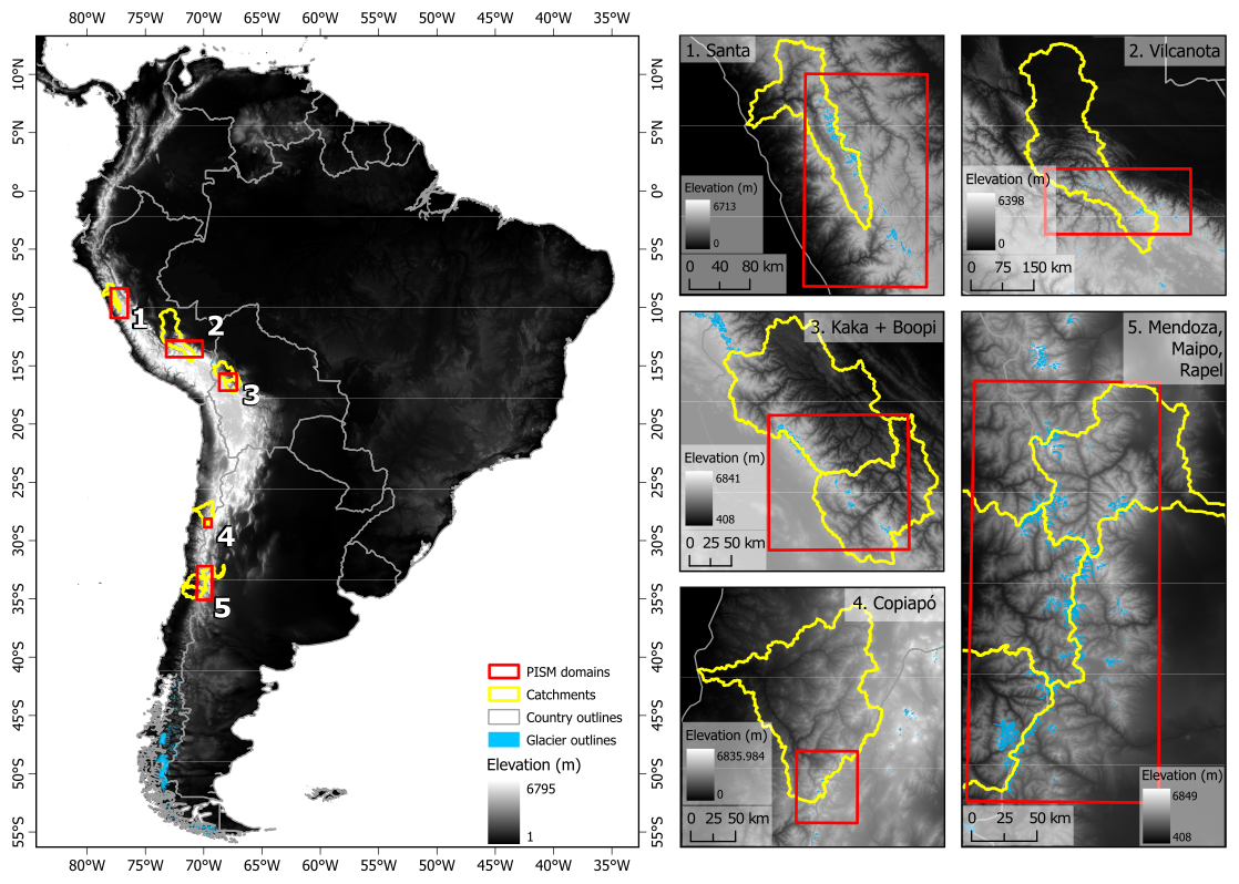
Figure 1 Chosen hydrological catchments and the five PISM domains across the South American Andean Mountains used in this sensitivity analysis. Red outlines show the model domains, focused on glacierized areas within each hydrological catchment. Hydrological catchment boundaries are from HydroSHEDS (Lehner et al., 2008). Elevation for each domain taken from the sub figure scene. The domain statistics are found in Table 2.

The Andes have been the focus of numerous studies examining glacier extent changes in response to both centennial (e.g., Carrivick et al., 2024; Emmer et al., 2021) and decadal scales (e.g., Dussaillant et al., 2019; Taylor et al., 2022). Global-scale studies using simplified two-dimensional flowline models (e.g., OGGM; Maussion et al., 2019) have modelled individual Andean glaciers as part of broader global modelling frameworks, which apply a uniform modelling approach across diverse climatic and topographic regimes. Although these global frameworks can assimilate regional climate data, they do not specifically optimise for Andean glacier dynamics and are unable to account for highly heterogenous climatic regimes such as those of Andean glaciers. However, regional-scale glacier modelling specific to the Andes remains limited. Most physically based modelling efforts have been concentrated on the Patagonian Icefields, a setting distinct from the rest of the Andes, while other studies are primarily focused on modelling from the Last Glacial Maximum to present (e.g., Cuzzone et al., 2024; Martin et al., 2022; Wolff et al., 2023; Yan et al., 2022). To date, only one study has focused in detail on modelling Andean Mountain glaciers outside Patagonia, assessing their response to climate extremes, however, this study is restricted to just two glaciers (Richardson et al., 2024). Consequently, parameter choices and process understanding for physically based modelling of Andean glaciers remain poorly constrained.

3 Materials and methods

3.1 Parallel Ice Sheet Model

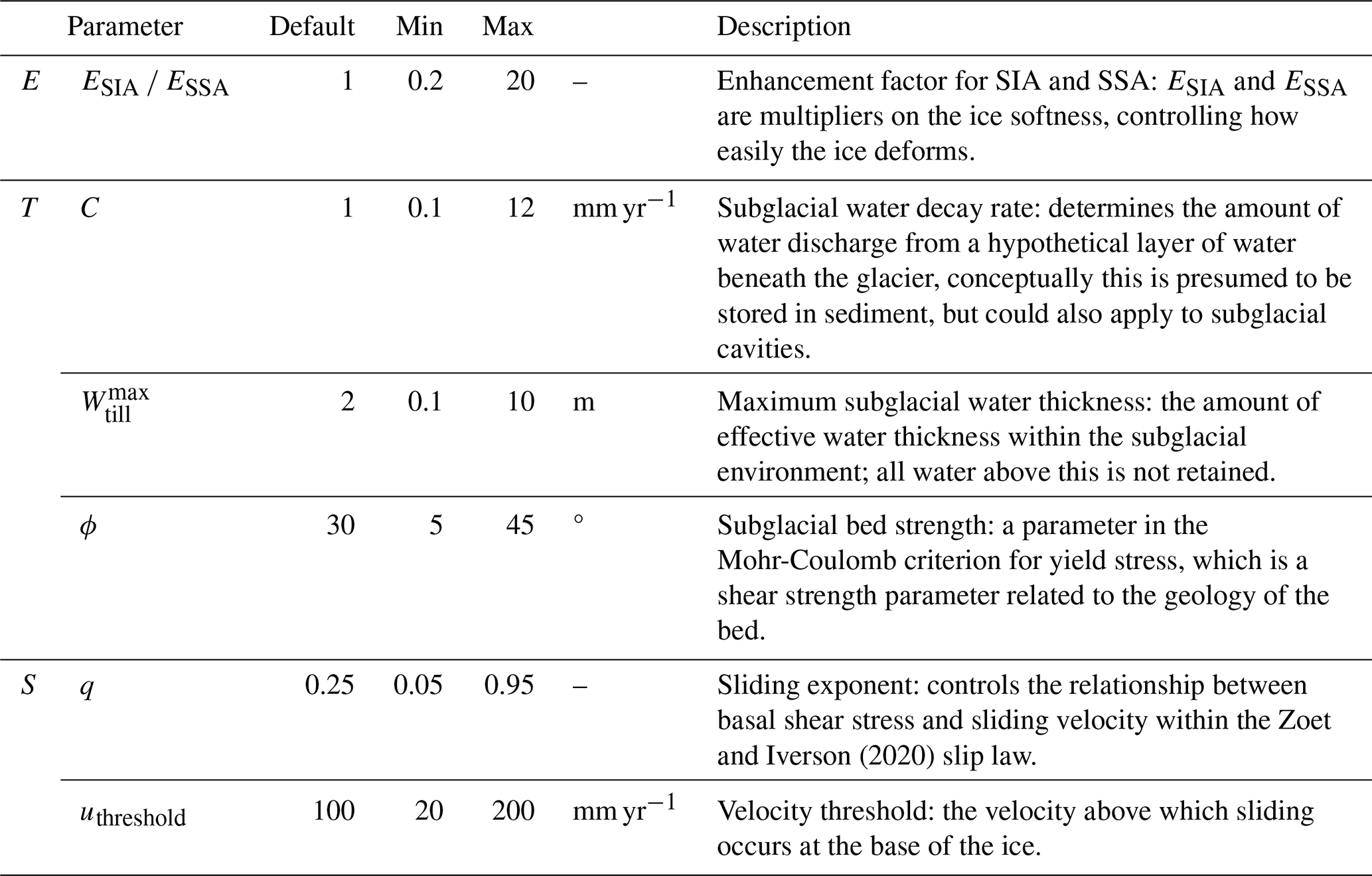
Here, we used the Parallel Ice Sheet Model (PISM v2.1) (Winkelmann et al., 2011) to conduct our numerical modelling. PISM is an open-source, three-dimensional, thermomechanically coupled, hybrid shallow ice, shallow shelf, approximation ice sheet numerical model. The parameter combinations of PISM can be calibrated to represent localised climate and glaciological conditions when sufficient observational constraints (e.g., mass balance data, surface velocity, past glacier extents) are known. Otherwise, default parameter values, which have primarily been tuned for the Greenland Ice Sheet, are set automatically if not specified. Key parameters we have chosen to change here are mentioned throughout the following sections and in Table 1, together with their PISM default values and the minimum and maximum values used in our sensitivity experiments. These ranges were informed by values used in previous modelling studies, as discussed below, but were deliberately extended beyond commonly applied ranges to test the response of model outputs under a wide parameter space.

Table 1 Chosen glaciological model parameters for sensitivity analysis within PISM. Letters on the leftmost edge of the table correspond to the component letter within PISM that the chosen parameters cover, the minimum and maximum values chosen are explained within the main text. Default values are those set within the PISM code. All other parameters not mentioned within this table are left at their default values, which can be found in PISM's Configuration Parameters online manual (https://www.pism.io/docs/manual/parameters/index.html, last access: 16 July 2026).

3.1.1 Enhancement Factors (E Component)

We used PISM's hybrid shallow ice shallow shelf approximation (hybrid SIA + SSA). This is the combination of the shallow-ice (SIA; Hutter, 1983; Mangeney and Califano, 1998) and shallow-shelf approximations (SSA; Bueler and Brown, 2009; Weis et al., 1999), enabling PISM to represent both the vertical deformation and longitudinal stretching of the ice, along with basal sliding. This hybrid SIA + SSA has been applied in other mountain valley-based glacial systems (e.g., Candaş et al., 2020; Golledge et al., 2012; Martin et al., 2022; Seguinot et al., 2018).

The stress balance, and the resulting rate of ice deformation ($\dot{\mathit{ϵ}}$), is described by the Glen-Paterson-Budd-Lilboutry-Duval flow law (Lliboutry and Duval, 1985). This is the default enthalpy-based flow law within PISM, shown in Eq. (1),

$$\begin{array}{}\text{(1)}& {\dot{\mathit{ϵ}}}_{ij}=EA\left(T,\mathit{\omega }\right){\mathit{\tau }}^{n-\mathrm{1}}{\mathit{\tau }}_{i,j}\end{array}$$

where E is the enhancement factor, A is the ice softness, T is the ice temperature, ω is the liquid water fraction, τ is the stress imposed on the ice, and n is the Glen's flow law exponent. E is implemented for both the SIA and SSA, acting as a multiplier on the ice softness inferred from A. Therefore, higher values are likely to represent softer ice that deforms more readily, while lower values of E represent stiffer ice.

For the sensitivity tests, we changed the parameterisation of E for both the SIA and SSA. Many studies have varied E_SIA with values between 1 and 6 (Candaş et al., 2020; Ely et al., 2024; Johnson et al., 2023; Zinck and Grinsted, 2022), and E_SSA between 0 and 1.5 (Martin et al., 2022; Seguinot et al., 2018; Yan et al., 2023). We varied both E_SIA and E_SSA at the same time between 0.2 and 20 (see Table 1). This wider range was used due to previous observations of E for SIA within lab studies have found values between 1.3 and 10.2 (Treverrow et al., 2012), and up to 120 in field studies over the Urymqi Glacier No. 1 in China (Echelmeyer and Zhongxiang, 1987). While no observations of E for the SSA are detailed, modelling studies (as shown above) have used narrower values. By applying an extended range to both E for SIA and SSA, we aim to test whether strongly reduced or enhanced deformation could substantially affect modelled output ice volume, thickness, and velocity, and therefore whether these parameters should be prioritised in future parameter ensembles.

3.1.2 Subglacial properties (T Component)

In PISM, the subglacial hydrology and sliding scheme was originally developed for ice-sheet contexts and conceptualises the bed as a deformable layer, to represent subglacial “till” or sediment, that can store water and influence basal resistance (Albrecht et al., 2020). We therefore refer to these parameters collectively as the “T component”, where “T” denotes till-related subglacial properties. The extent to which this subglacial sediment is under ice sheets is unknown, which is also the case for Andean glaciers (Cuffey and Paterson, 2010). Although, thick layers of sediment are common in mountain glacier forefields due to repeated glacier advance and retreat phases, and meltwater reworking (e.g., Carrivick and Heckmann, 2017, Lee et al., 2022). However, the formulation for glacier sliding and hydrology does not require, and should not be interpreted as, sediment to be present everywhere beneath the glacier. The effective pressure and sliding behaviour can equally represent hard-bedded conditions, where subglacial water storage may occur within bedrock cavities rather than within sediments (Cuffey and Paterson, 2010; Zoet and Iverson, 2020). Therefore, while we use the term “till” throughout this study for consistency with PISM terminology and previous studies, it should not be interpreted as implying continuous sediment cover beneath Andean glaciers.

The yield stress of the basal material (τ_c) in PISM is calculated using the Mohr-Coulomb criterion, which incorporates the till friction angle (ϕ), a parameter influenced by the underlying bed geology (Albrecht et al., 2020; Cuffey and Paterson, 2010). This relationship is partly governed by PISM's subglacial hydrology model. The Mohr-Coulomb criterion used to compute yield stress is given in Eq. (2),

$$\begin{array}{}\text{(2)}& {\mathit{\tau }}_{\mathrm{c}}=c_{\mathrm{0}}+\left(\tan \mathit{\varphi }\right)N_{\mathrm{till}}\end{array}$$

where c₀ is the till cohesion that uses a default value of 0 (Schoof, 2006), and N_till is the effective pressure at the base of the ice within the till layer. For every domain we applied a spatially uniform ϕ. Previously used values of ϕ have generally been within ranges of values 5–45°, derived from lab-based experiments of different till types (Cuffey and Paterson, 2010; Koloski et al., 1989). Lower values of ϕ represent a weak, slippery bed that promotes basal sliding due to a low yield threshold, while higher values represent a strong, rigid bed that increases basal friction and makes sliding harder to occur. The default value in PISM is 30°, while in the sensitivity tests, we varied ϕ between 5 and 45° (see Table 1).

Within Eq. (2), N_till is determined in part by the hydrology beneath the ice. The hydrological model used here is a non-conserving model (Tulaczyk et al., 2000). This does not allow the conservation of any water above an assigned till water thickness ($W_{\mathrm{till}}^{\max }$). This is where W_till is constrained between 0 and the prescribed $W_{\mathrm{till}}^{\max }$ value. Any water exceeding this is removed from the till water layer and is not retained. The thickness of the water layer stored within the till is determined by Eq. (3),

$$\begin{array}{}\text{(3)}& {\displaystyle \frac{\partial W_{\mathrm{till}}}{\partial t}}={\displaystyle \frac{m}{{\mathit{\rho }}_{\mathrm{w}}}}-C\end{array}$$

where m is the basal melt rate, ρ_w is the density of fresh water (1000 kg m⁻³), and C is the till water decay rate that denotes how fast water is evacuated from the till water (Albrecht et al., 2020; Flowers, 2015).

C and $W_{\mathrm{till}}^{\max }$ are tested in our sensitivity analysis through the T Component. To our knowledge, no previous PISM studies have varied C over mountain glaciers, although PISM ice sheet studies have used values between 1 to 10 mm yr⁻¹ (Albrecht et al., 2020). Higher values of C drain the till faster, analogous to efficient drainage systems, that is likely to cause less sliding overall, while lower valuers of C represent a more inefficient drainage, leading to more water within the till and likely allowing more sliding to occur. Here we vary C between 0.1 and 12 mm yr⁻¹.

For $W_{\mathrm{till}}^{\max }$ previous PISM mountain glacier studies have used values between 1 to 5 m (Candaş et al., 2020; Žebre et al., 2021). High values of $W_{\mathrm{till}}^{\max }$ allow more water to be retained within the till at the base of the ice. The $W_{\mathrm{till}}^{\max }$ is varied between 0.1 and 10 m (see Table 1). These ranges either extend beyond previously used values for mountain glacier modelling studies, or applied ranges that have been used over ice sheet scales, aiming to assess whether either parameter has a substantial influence on modelled output of ice volume, thickness, or basal velocity.

3.1.3 Basal sliding (S Component)

In PISM, basal sliding is represented by relating the basal shear stress (τ_b) to both the ice velocity (u) and effective pressure (N). A velocity threshold (u_threshold) marks when τ_b equals the yield stress (τ_c), and therefore when sliding occurs (Cuffey and Paterson, 2010). Within PISM we used the Zoet and Iverson (2020) slip law, which introduces a regularisation term that enables a smooth transition between the viscous-style Weertman sliding (Weertman, 1957), and the Coulomb-plastic behaviours (Aschwanden et al., 2013), without needing prior knowledge of bed type. The Zoet and Iverson (2020) slip law is expressed in PISM by Eq. (4),

$$\begin{array}{}\text{(4)}& {\mathit{\tau }}_{\mathrm{b}}=-{\mathit{\tau }}_{\mathrm{c}}{\displaystyle \frac{u}{{\left(\left|u\right|+u_{\mathrm{threshold}}\right)}^q{\left|u\right|}^{\mathrm{1}-q}}}\end{array}$$

Zoet and Iverson (2020) in their equation parameterise $q=\mathrm{1}/m$ where m= 5, whereas PISM's default value of q is 0.25 (or where m= 4). While the Zoet and Iverson (2020) slip law is relatively new in PISM, being introduced in v2.0, few PISM studies have utilised it. Those modelling efforts that have used the Zoet and Iverson (2020) slip law, (e.g., the Community Ice Sheet Model or CISM; Lipscomb et al., 2019), have varied it between narrow ranges. These have been at 0.2 (Khan et al., 2022; Moreno-Parada et al., 2023), 0.23 (Maier et al., 2022), or 0.33 (van den Akker et al., 2025; Hoffman et al., 2022; Joughin et al., 2024). Within our sensitivity analysis, q and u_threshold were tested through the S component.

We varied q from 0.05 to 0.95 to maximise the coverage of potential parametrisations of q to the extremes. Due to the use of the Zoet and Iverson (2020) slip law in this study, increasing the value of q can lead to decreased resistance were there are low to moderate basal velocities, or where it is near the onset of sliding, increasing velocities in those areas. Where there are the fastest velocities (i.e., ice flowing into valleys), there is likely to be minimal effect on their velocities due to basal shear stress already being at, or near, to the yield stress.

We also varied u_threshold, a parameter that has seen variation for sensitivity or optimisation within a limited number of studies to our knowledge. Bevan et al. (2023), applied the BISICLES ice sheet model to the Amundsen Sea Embayment in West Antarctica, used values between 20 to 600 m a⁻¹. Due to the u_threshold only being varied over ice sheet settings, we varied the u_threshold between 20 and 200 m a⁻¹ (see Table 1). The maximum value we use takes into account the mountain glacier setting we are studying: mountain glaciers are unlikely to reach the high velocities that are achieved by ice streams (> 200 m a⁻¹). It is anticipated that higher parameter values for u_threshold would lead to sliding occurring over less of the glacier, but higher maximum basal velocities. Higher thresholds will delay the transition to Coulomb-limited sliding, but once the threshold is exceeded, higher sliding velocities will occur. Conversely, decreases in the u_threshold are likely to lead to larger portions of the glacier experiencing sliding, but lower maximum velocities.

3.1.4 Surface mass balance

We used PISM's default positive degree day (PDD) temperature-index scheme (Calov and Greve, 2005) to generate ice within the domains. This required monthly mean air temperature and yearly precipitation (see Sect. 3.3).

Within the PDD scheme, there is stochastic “white noise” to simulate additional undetermined daily variability, as well as a daily temperature standard deviation that is set by default at 5 °C (Winkelmann et al., 2011). We acknowledge that the treatment of sub-monthly temperature variability within the PDD model can influence simulated melt and is therefore another source of uncertainty within the model (Seguinot, 2013).

We forced the model with a constant present-day climate (see Sect. 3.3), to allow glacial ice to reach steady state with its surrounding climate. As this study is focused on purely parameters that influence ice flow, parameters that affect the PDD model component of PISM, such as degree day factors, were kept at their default values and not varied within this study. Any minor fluctuations in steady-state ice extent associated with the PDD scheme are consistent across the ensemble and do not affect the relative comparison between ice-flow parameter perturbations.

3.2 Model setup and parameter sensitivity analysis

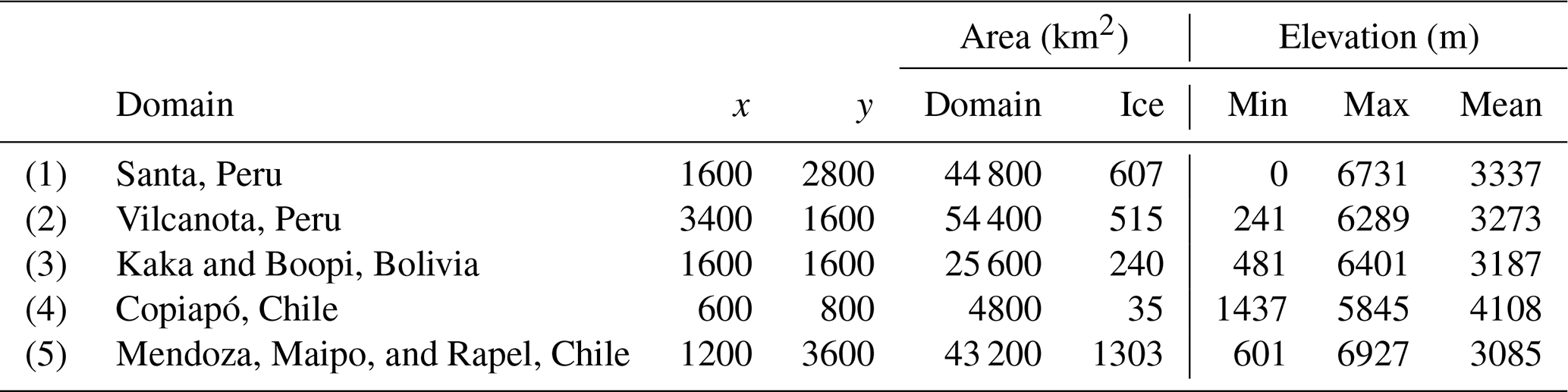
The five model domains simulated by PISM are shown in Fig. 1. Each domain had a 100 m horizontal grid resolution (dimensions in Table 2), with 50 vertical ice layers spaced quadratically, and 10 bedrock layers. These vertical layers were chosen to resolve near-basal ice interactions where thermal and sliding-related processes are important, further this horizonal resolution was chosen as it can resolve the topography and flow characteristics while maintaining feasible wall-clock run times (e.g., Lee, 2024). No separate sensitivity test was performed for vertical and horizonal resolution set up, however this was kept the same for all model runs. All domains were initialised without prescribed ice thicknesses, allowing mountain glaciers to grow from no ice conditions, and run to steady state (∼ 1500 model years) under constant climate forcing (see Sect. 3.2).

Table 2 PISM study domains, detailed with their grid x, y, the domain area, the RGIv7 ice area, and the elevations from the ALOS DEM, for each domain all at 100 m resolution. The location of each domain, and the hydrological catchments they cover, are shown in Fig. 1.

Our sensitivity analysis focused on internal ice-flow parameters. These parameters define the physical properties and processes governing ice behaviour, such as the shallow ice, and shallow shelf approximation (SIA/SSA) flow enhancement factor, basal sliding, and subglacial mechanics. We targeted parameters that: (i) have shown substantial influence on glacier modelling in previous studies; (ii) are commonly tested in sensitivity analyses; and (iii) remain poorly constrained by observations or past modelling.

The analysis followed a two-stage approach (Fig. 2) to enable efficient identification of components that exert the greatest control over model outputs. This coarse screening (Stage 1) allowed subsequent parameter-specific tests (stage 2) to focus only on the most sensitive components governing ice flow. This aim of this is to reduce the dimensionality of the analysis and the computational cost of future ensemble experiments. This two-stage approach can be used by other sensitivity studies to facilitate more efficient sampling of key aspects of the model in question that causes the most effect on chosen outputs.

In stage 1 (135 model simulations: 27 per domain), we group individual parameters into components impacting three key ice-flow processes: enhancement factors (E), basal sliding (S), and subglacial properties (T). The parameter values applied span beyond those commonly used to capture a broad spectrum of glacier responses, see Sect. 3.1 for details. Each component was perturbed between its chosen minimum, maximum, and default values (Table 1), first individually (with all other components fixed at default values) and then simultaneously, to generate the ensemble design for each domain (see Table S1 in the Supplement for an example). Components that showed negligible influence on outputs were discarded from further analysis.

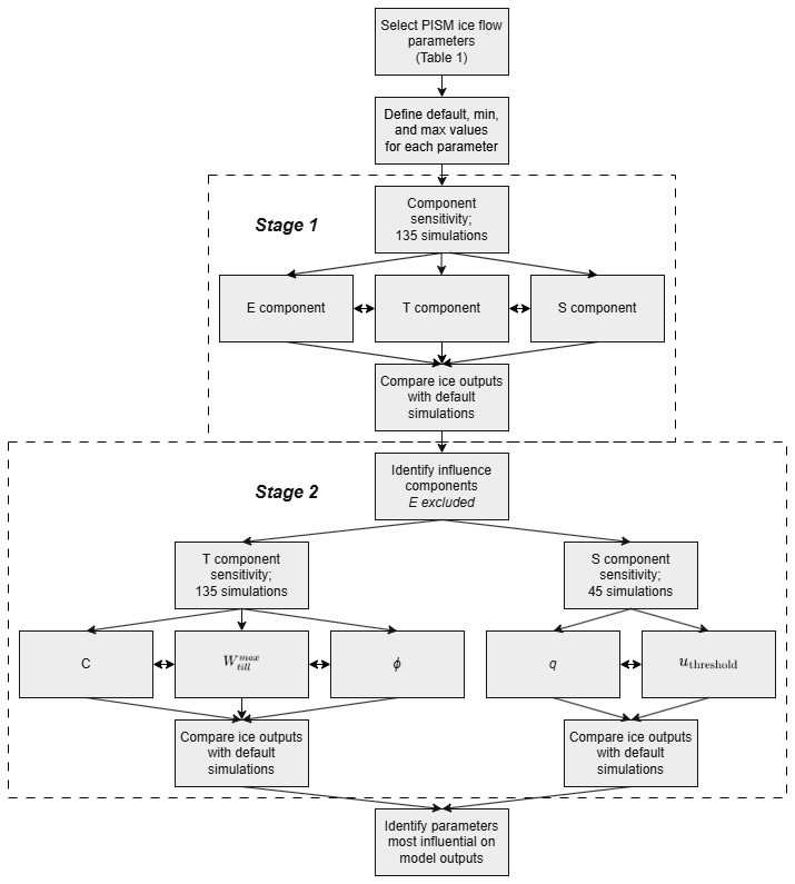
Figure 2 Workflow of the two-stage sensitivity experiment design used here. Stage 1 tests the influence of the chosen model components; the enhancement factors (E), till-related parameters (T), and sliding parameters (S). These use the default, minimum, and maximum parameter values from Table 1. Components with limited influence are excluded from Stage 2. Stage 2 then tests individual parameters within the retained T and S components to identify which parameters exert the most influence on modelled ice volume, thickness, and basal velocity. Simulation numbers are shown for the full five-domain ensemble. These were varied both individually and all together.

Stage 2 (180 model simulations: 36 per domain) comprised a detailed within-component analysis of only those components identified in Stage 1 as influential. Here, every individual parameter was perturbed one-at-time across their defined value ranges (min, max, default; Table 1), followed by simultaneous perturbation of all parameters within that component, rather than grouping them by component as in Stage 1. Parameter in each figure and table corresponds to a shortened name presented here; enhancement factor (E), till water decay rate (C), maximum till water thicknesses (Tm or $W_{\mathrm{till}}^{\max }$), till friction angle (Phi or ϕ), sliding exponent (q), velocity threshold (Uth or u_threshold).

Model outputs, of ice volume, ice thickness, and basal velocity, were compared against the baseline simulation using the default values for all parameters. To quantify influence, results were averaged over the domain and Pearson correlation coefficients were calculated between these and the parameter values, along with p-values to assess statistical significance of their effect. This approach provided both a ranking of parameter sensitivity and an assessment of the robustness of their effects.

3.3 Boundary conditions data

Topography is a key initial condition within PISM. We used the ALOS 30 m DEM (Tadono et al., 2014), due to its accuracy over complex mountainous terrain (Talchabhadel et al., 2021), resampled to 100 m using a bilinear interpolation. Basal topography was derived by subtracting present-day ice thicknesses of Millan et al. (2022) from the ALOS DEM.

Geothermal heat flux is required to define and apply the temperature of the bed to the base of the ice. Geothermal heat flux was prescribed from Davies (2013) which uses the relationship between basal heat flux to geology on a 2° × 2° global grid. Due to the lack of regional specific geothermal heat flux estimates within our study areas and the coarse nature of the dataset, for each domain we assigned a single value based on the value from the grid cell containing the most glacial ice.

Climate input is required for the PISM PDD scheme. For our present-day climate, we used the WorldClim 2.1 data (Fick and Hijmans, 2017). WorldClim 2.1 is a gridded climate data for the years 1970–2000 collected from weather stations here we use the average air temperature (K) and average total annual precipitation (mm yr⁻¹), resampled from a grid resolution of ∼ 900 to 100 m bilinearly. Due to air temperatures from WorldClim being based on the 3 arcsec SRTM DEM, it underestimates temperatures across mountain peaks. To remedy this, we applied the global average lapse-rate correction of 6.5° C km⁻¹ across the entire temperature field, based on elevation differences between the WorldClim SRTM and resampled ALOS DEMs. Erroneous adjustments due to DEM artefacts were removed and interpolated across linearly. We acknowledge that the chosen lapse rate correction of the temperature field can itself present some uncertainty. Ultimately, the purpose of the climate forcing in this study is not to reproduce the exact present-day size and shape of each glacier, but to generate steady-state ice extent within each domain from which we can determine the sensitivity to ice-flow parameters.

4 Results and Discussion

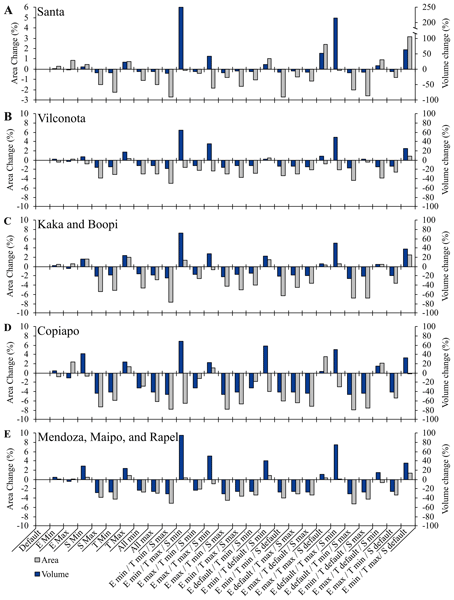
Here, we outline results from the Stage 1 component sensitivity experiments for simulated volume change, then for the subsequent Stage 2 parameter sensitivity experiments, for all domains. Aggregated domain results are shown here, with individual model simulation outputs (area, volume, and percentage changes for each domain) available in the Supplement: component sensitivity (Tables S1–S5), subglacial parameter sensitivity (Tables S6–S10), and sliding parameter sensitivity (Tables S11–S15). Final time-slice outputs of ice thickness and ice velocities, along with their differences with the default model simulation for their respective regions, are shown in Figs. S1–S40. Key examples of these are shown throughout which are also shown in the Supplement for ease of comparison. Ice area was largely unaffected by parameter changes. We therefore include area within the sensitivity bar graphs for transparency but focus the main discussion on ice-volume change.

4.1 Stage 1 – Model component sensitivity analysis

Stage 1 is used to determine which model component influences the ice metrics the most, to guide the more detailed Stage 2 sensitivity analysis (Table 3; Fig. 3). We describe results for each component in turn here.

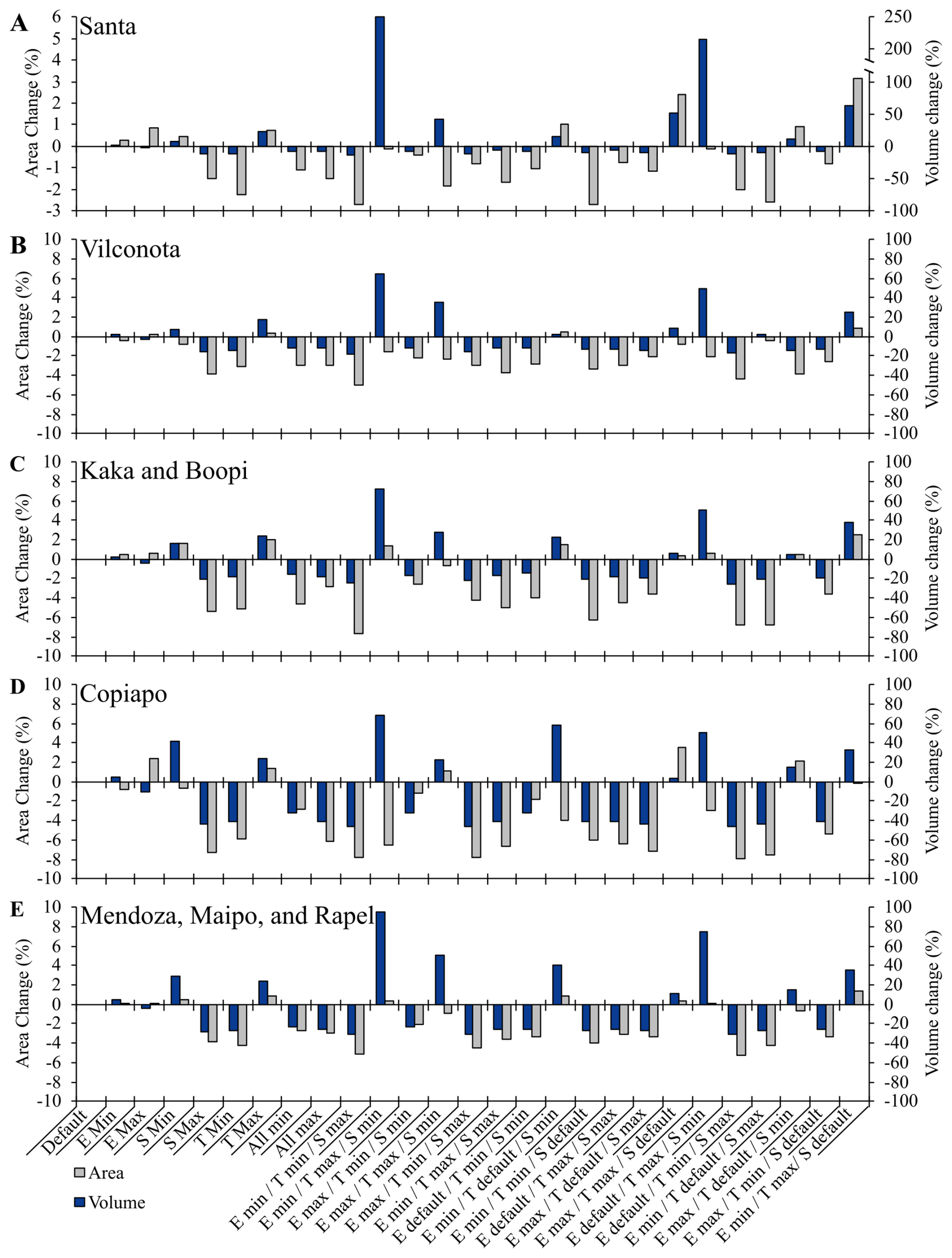
Figure 3 Initial sensitivity analysis detailing the area (grey) and volume (blue) absolute change percent due to changing all model component parameters together, for each of the five model domains. Blue and grey lines denote the default volume and area respectively for comparison. Component parameters are: E= enhancement factors, T= subglacial component, S= sliding component. See Fig. 1 for model domain locations. Note the break in y-axis for ice volume in (A) detailing the significant increase in volume, above + 200 %.

When varying E component parameters (E_SIA and E_SSA) between their minimum and maximum values (Table 1) resulted in ice volume changes of + 5.4 % to − 9.9 % from their defaults across all domains. These changes are reflected primarily in ice thickness (Fig. 4), with maximum E values producing thinner ice (mean: − 5.4 %) and increased basal velocities (mean: + 4.8 %), though the Vilcanota (#2) domain showed a velocity decrease of − 11.9 %. Minimum E values led to thicker ice (mean: + 3.2 %) and reduced velocities (mean: − 9.1 %). Pearson correlations between E and ice volume were weak and statistically insignificant across all domains (p> 0.53; Table 4).

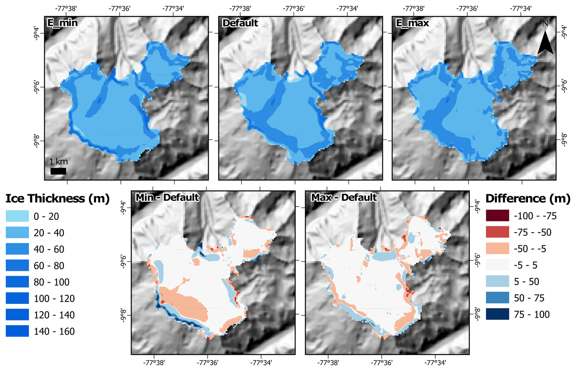
Figure 4 Example of the influence of the enhancement factors on simulated ice thickness in the Santa (#1) domain (Huascarán Ice Cap). Additional examples are provided in the Supplement. Ice peripheral differences in ice thickness are likely to arise from internal variability in the PDD model as mentioned previously in Sect. 3.3. Parameter values for “max” and “min” are listed in Table 1.

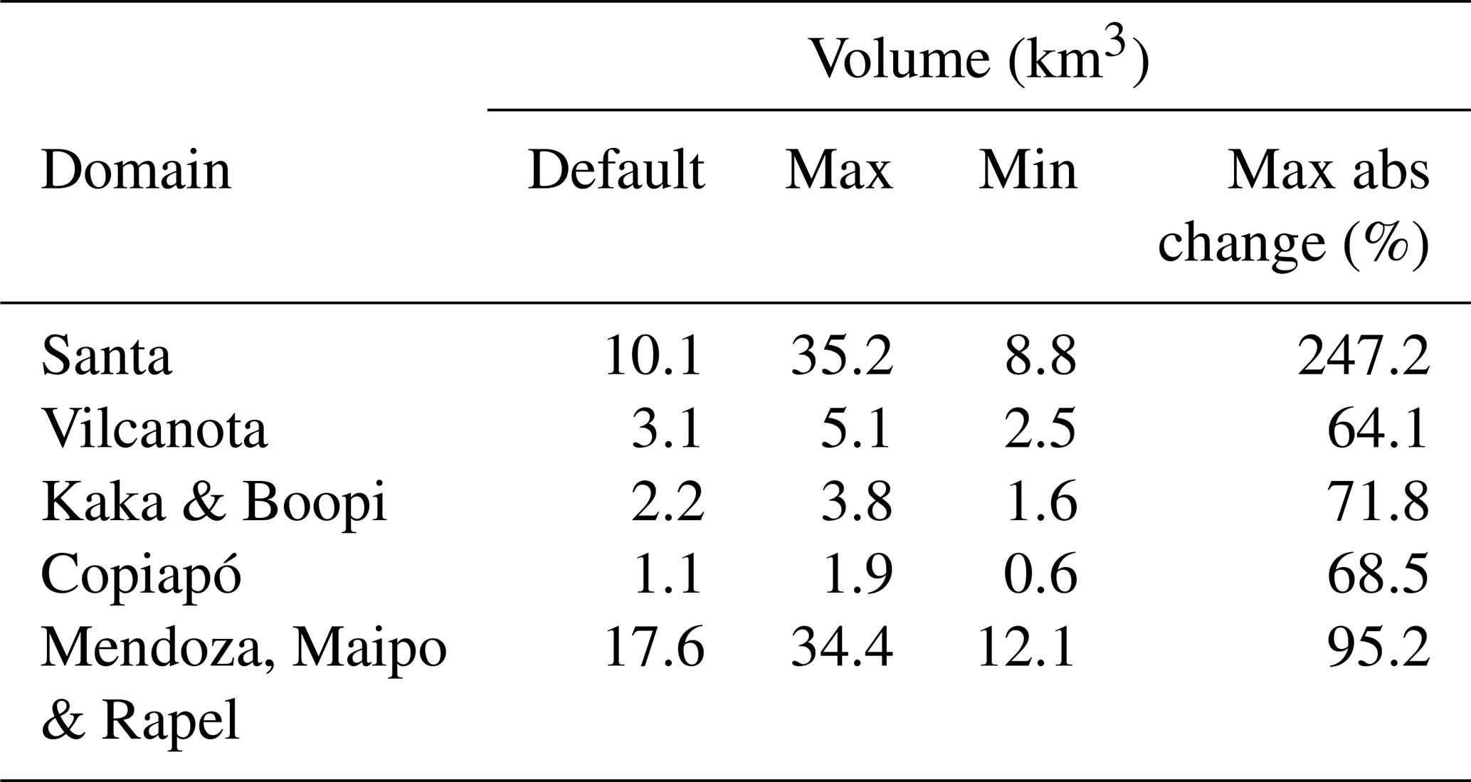
Table 3 Initial sensitivity analysis outputs detailing the default model simulation volume, and the maximum absolute percentage changes for volume for each domain across the ensemble when components were varied between their maximum and minimum values.

Similar results – i.e., non-significant variations in modelled outputs – were reported using PISM in other mountain glacier settings (Candaş et al., 2020; Martin et al., 2022) and for ice caps (Schmidt et al., 2020). More substantial effects from the enhancement factors that impact ice rheology, have been observed in models of ice sheets (e.g., Lowry et al., 2020; Phipps et al., 2021; Pittard et al., 2022). Given the minimal impact of enhancement factors in this study, they were excluded from the Stage 2 sensitivity analysis.

When the T component parameters (subglacial water decay rate, maximum subglacial water thickness and bed friction angle) were varied between their minimum and maximum values (Fig. 3; Table 1) resulted in volume changes of − 40.5 % to + 23.6 % from their defaults across all domains. Minimum T parameter values increased basal sliding velocities substantially: up to + 213.4 % in the Copiapó (#4) domain (Fig. S12), a mean of + 62.4 % across all domains, leading to a mean ice thickness reduction of − 20.9 %. In contrast, maximum T parameter values reduced mean basal velocities by − 49.2 %, resulting in a mean thickness increase of + 22.5 % (Fig. 5). The resultant difference in the ice velocities and ice thicknesses can be seen in the shift of the ice divide, being primarily constrained to the glacier valley, to being more diffuse with minimal T component values, and being significant muted with maximum T component values.

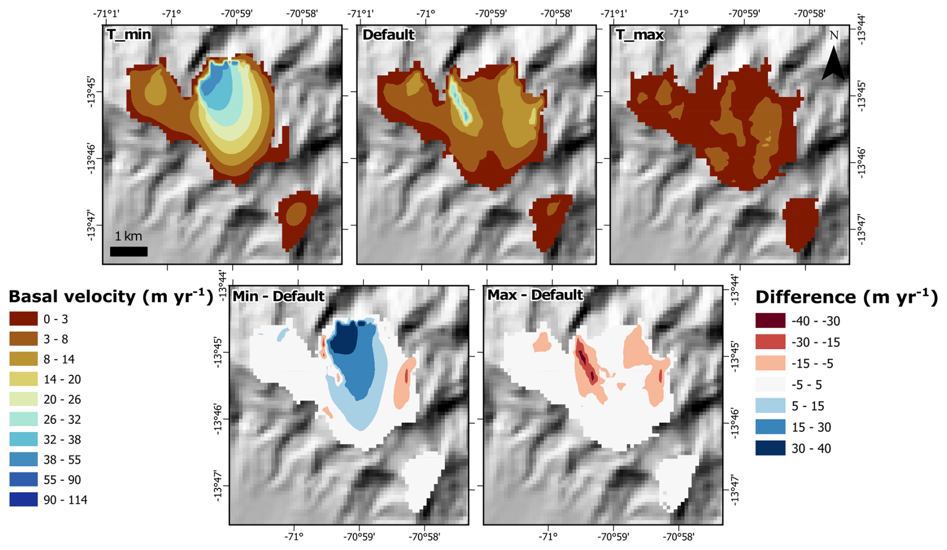
Figure 5 An example of the influence of the subglacial component chosen parameters on the output of ice basal velocity in Vilcanota (#2) domain (Quelccaya Ice Cap). Remaining examples are shown in the Supplement. Increased values of the chosen parameters generate reduced basal ice velocities, while decreasing values increase them. This can also lead to changes in ice divides as seen in T_min, compared to T_max. Values that correspond to “max” and “min” parameter values are found in Table 1.

When the S component parameters (sliding exponent and velocity threshold) were varied between their minimum and maximum values (Table 1) resulted in ice volume changes of − 43.2 % to + 41.2 % (Fig. 3) from their defaults across all domains. Minimum S parameter values reduced basal velocities by a mean of − 24.4 % across all domains (− 79.5 % in the Copiapó domain), resulting in thicker ice (mean: + 15.5 %). Conversely, maximum values increased basal velocities by a mean of + 47.7 % (+ 235 % in the Copiapó domain), leading to thinner ice with a mean of − 17.3 %. The larger percentage volume changes of the Copiapó domain reflect its low ice cover as small changes to the already small volume of ice (1.1 km³) yields large relative differences.

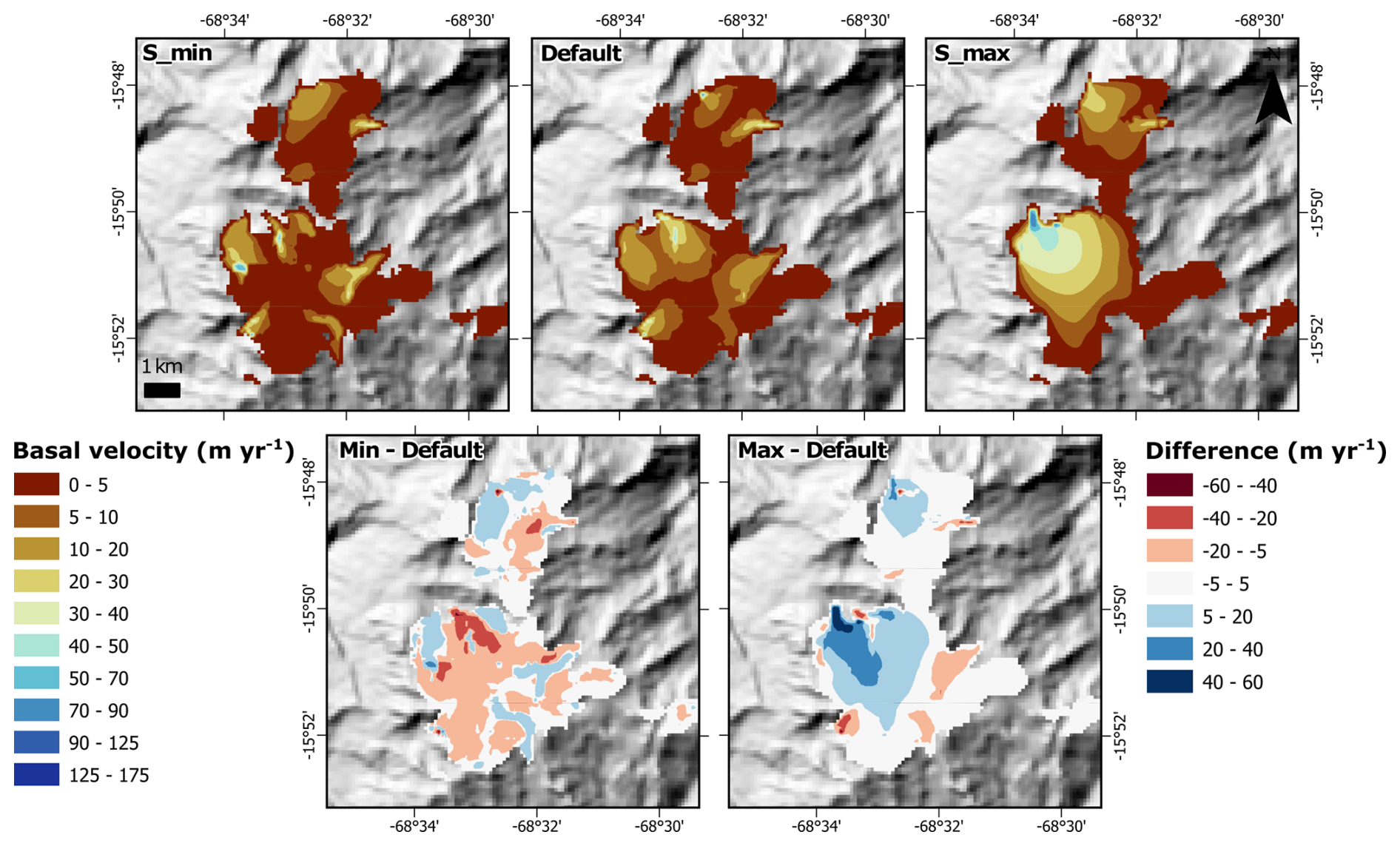
Figure 6 Example of the influence of sliding component parameters on basal ice velocity in the Kaka & Boopi (#3) domain (Ancohuma Ice Caps). Additional examples are provided in the Supplement. Increased parameter values enhance basal velocities, while decreased values reduce them. Variations amplify or suppress sliding patterns already present in the default simulation. “Max” and “min” parameter values are listed in Table 1.

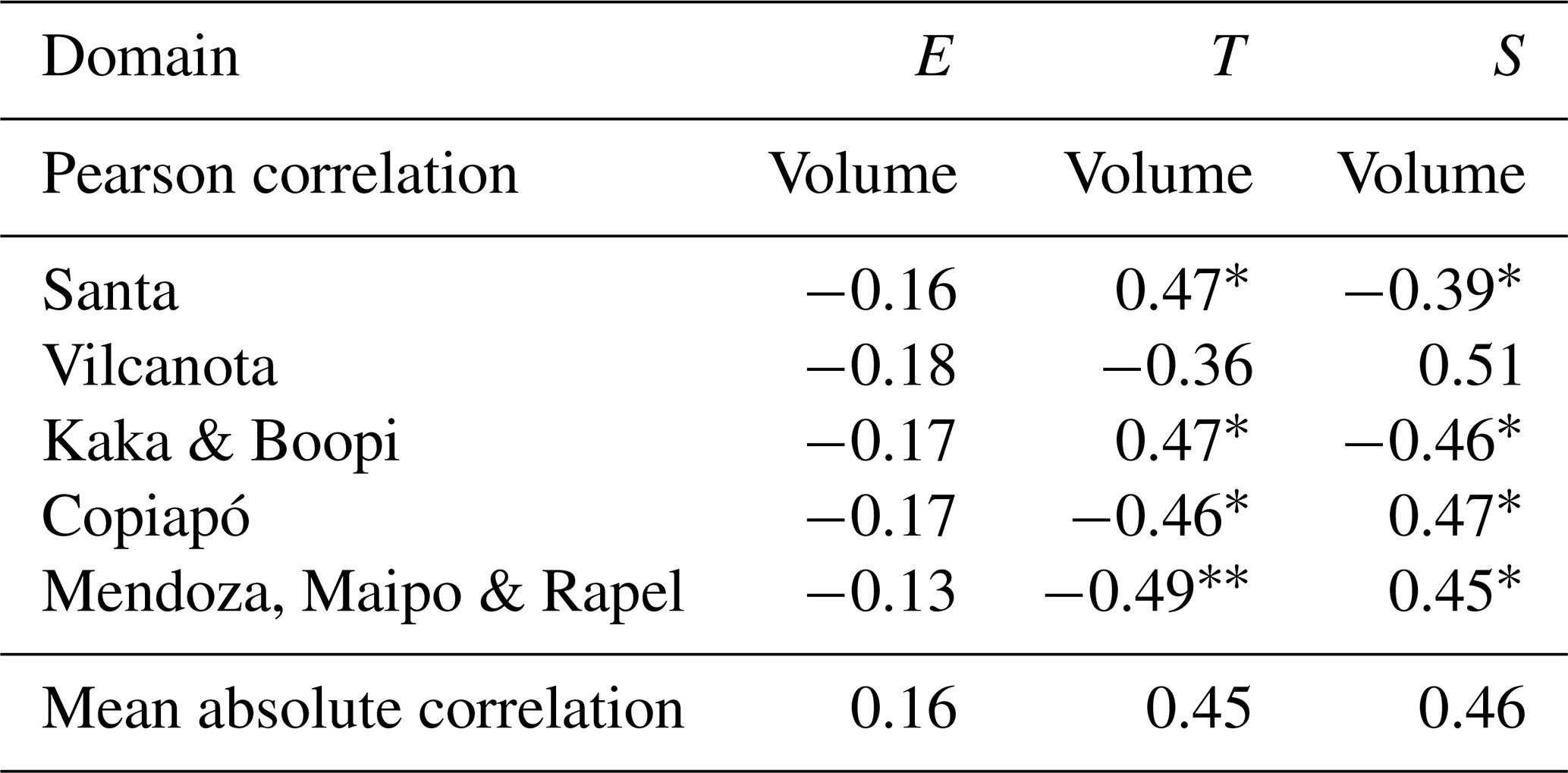
Collectively varying all parameters of the E, T, and S components between default, minimum, and maximum values (Table 1) produced a maximum mean ice volume increase of + 109.3 % across all five domains (Santa domain max: + 247.2 %), driven by the {E_min, T_max, S_min} combination (Fig. 3). The second highest mean increase of + 89.3 % (Santa domain max: + 221.3 %) resulted from {E_default, T_max, S_min}. Averaging across all combinations that include T_max or T_min produced mean ice volume changes of + 33.6 % and − 22.6 %, respectively, while those that include S_max or S_min produced changes of + 38.6 % and − 23.2 % respectively. Pearson correlation analysis (Table 4) confirms a strong and significant correlations (p≤ 0.05) for the T and S components and their effects on simulated ice volume in almost all domains.

Table 4 Pearson correlation statistics for all domains (n= 27 simulations per domain, 135 simulations overall) to understand the impact of model components on simulated ice volume. A value closer to zero (0) indicates a lower influence on the simulated volume output. A positive or negative number indicates that when the component value is varied it causes a gain or loss of simulated ice volume. The final row reports the mean absolute Pearson correlation across domains and is intended only as a descriptive summary of relative parameter influence, not as a formal regional statistic. ^* $=p\le$ 0.05, ${}^{**}$ $=p\le$ 0.01.

Given its limited influence on simulated ice volume, the enhancement factors (E) with E_SIA and E_SSA parameters, is excluded from the individual parameter sensitivity analysis of Stage 2. The subglacial (T) and sliding (S) components demonstrated significant impacts through both univariate and multivariate perturbations and were included in the Stage 2 sensitivity experiments (Sect. 4.2).

Remarkably, between different domains the relative importance of parameters remains remarkably consistent (Fig. 3), although the magnitude of influence varies (e.g. Table 4). These intra-domain variations are likely an impact of different domain boundary conditions and settings. For instance, glacier size is likely to play a key role. The smallest domain, Copiapó, with also the smallest area of glacial ice, often showed large relative percentage changes because its default ice volume was small, meaning that modest absolute changes in ice thickness or extent produced proportionally large changes in model outputs. Conversely, larger and more glacierised domains, such as the Mendoza, Maipo, and Rapel domain, provided a broader range of glacier geometries and flow dynamics, producing a more complicated response to parameter perturbations. Climatic setting may also have influenced the magnitude of area and volume change for different parameter sets. Further work, varying the climate input for a given domain, is required to explore any potential interaction between ice flow parameters and climatic variables.

4.2 Stage 2 – Individual parameter sensitivity analysis

4.2.1 Subglacial model parameters (T Component)

The T component parameter tests investigated the subglacial water decay rate (C), the maximum thickness of subglacial water ($W_{\mathrm{till}}^{\max }$), and basal friction angle (ϕ). Summary statistics for the T component tests are presented in Table 5 and Fig. 7. Among all domains when the parameters were varied, the Copiapó domain, being the smallest, exhibited the largest change in simulated ice volume (− 40.5 %). The second largest change (+ 28.3 %) occurred in the Mendoza, Maipo and Rapel domain, the largest and most ice-rich domain.

Table 5 Overall, subglacial sensitivity analysis outputs detailing the default model simulation volume, and the maximum absolute percentage changes for volume for each domain across all the model simulation when components were varied between their maximum and minimum values.

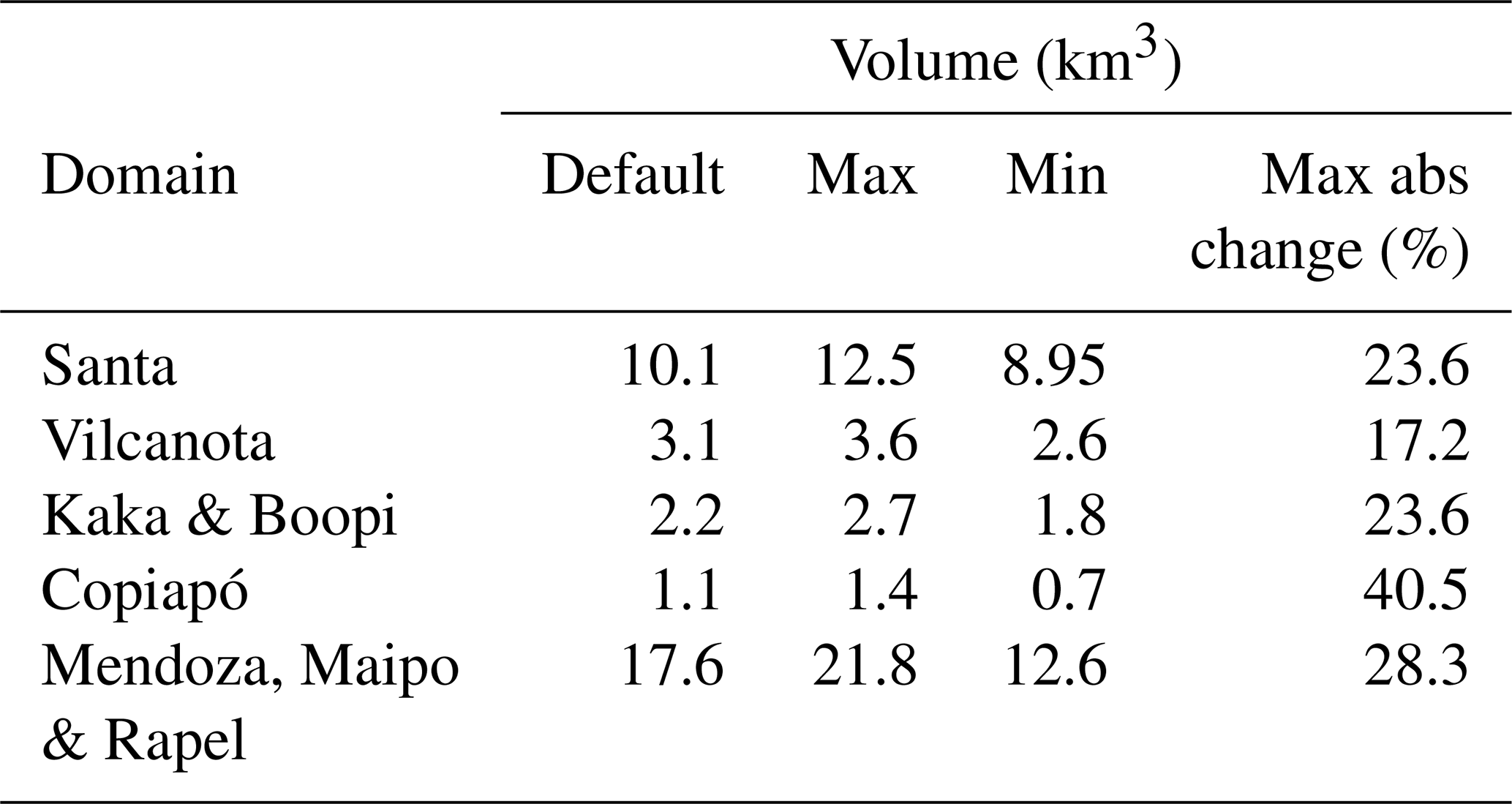
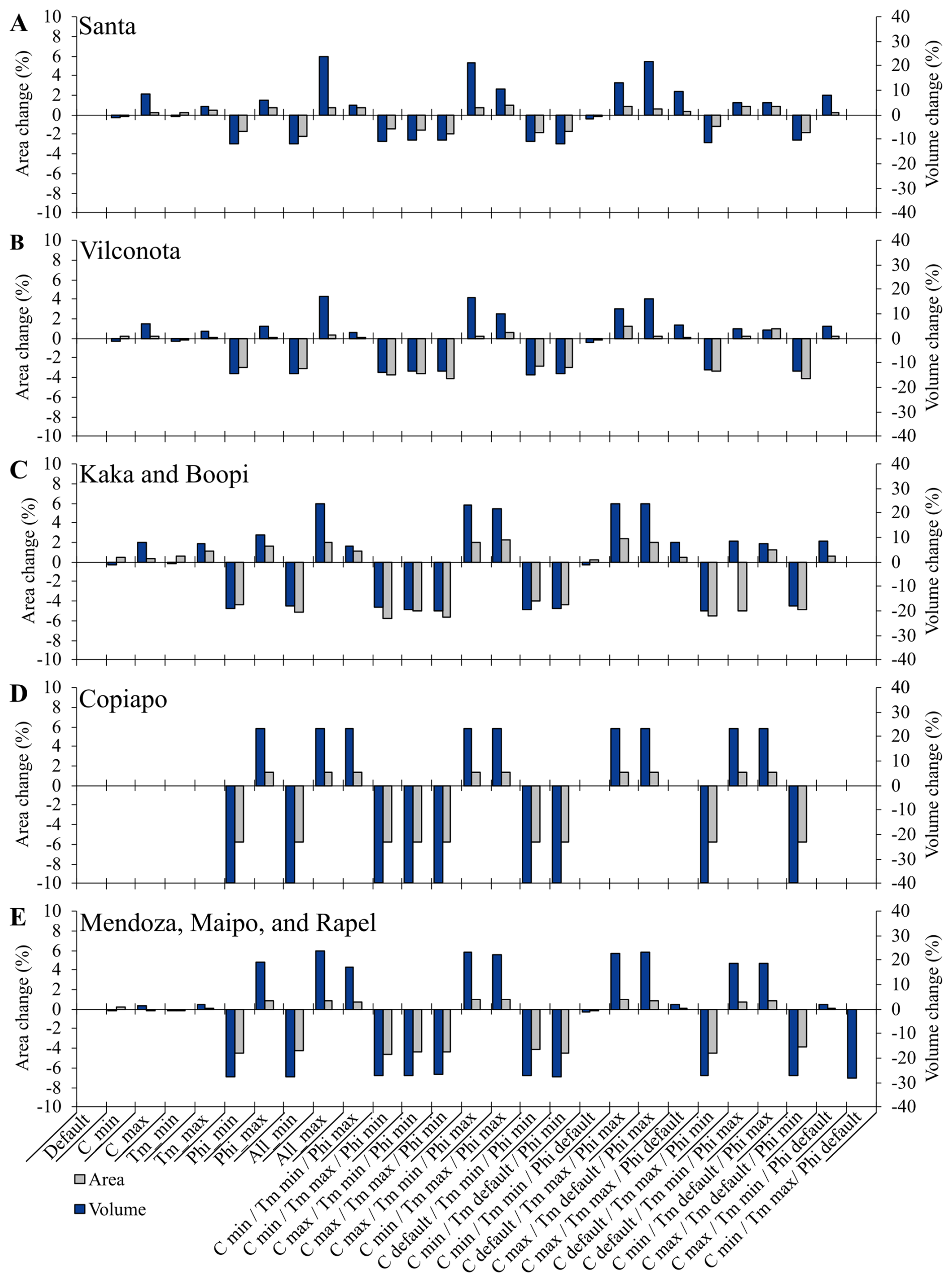
Figure 7 T sensitivity analysis detailing the area (grey) and volume (blue) absolute percentage changes due to changing the model component parameters all together, for each of the five model domains. Blue and grey lines denote the default volume and area respectively for comparison. Where there is no bar present for the component parameter, there was no change (0 %). Subglacial parameters are, C= basal water decay rate, Tm = $W_{\mathrm{till}}^{\max }$, Phi =ϕ. See Fig. 1 for domain locations.

Varying the subglacial water decay rate (C) between its minimum and maximum values (Table 1) resulted in ice volume changes of − 1.4 % to + 8.6 % respectively across most domains. No change was observed in the Copiapó domain. This may reflect the small glacierised area within this domain, where changes in subglacial hydrological parameters have limited influence on domain-mean outputs. It may also reflect the simplified representation of subglacial hydrology in PISM, which may not fully resolve hydrological variability beneath small mountain glaciers at the model resolution used here. Ice thickness and basal velocity changes across all domains were minor or negligible (e.g., no change in the Copiapó domain, Fig. S25). Minimum C values slightly reduced ice thicknesses (mean: − 1.0 %) and increased velocities (mean: + 1.6 %, − 7.5 % in the Vilcanota domain). Maximum C values increased thickness (mean: + 5.1 %) and decreased velocities (mean: − 14.6 %), reflecting the larger deviation of the maximum (12 mm yr⁻¹) from the default (1 mm yr⁻¹) relative to the minimum (0.1 mm yr⁻¹).

When $W_{\mathrm{till}}^{\max }$ was varied between its minimum and maximum values (Table 1), it resulted in ice volume changes of between −1.0 % to + 7.7 % across all domains (Fig. 7). No changes were seen across the Copiapó domain. Minimum $W_{\mathrm{till}}^{\max }$ saw minimal reductions in ice thickness (mean: − 0.2 %) and increases in velocity changes (mean: + 3.3 %), while maximum $W_{\mathrm{till}}^{\max }$ provided slightly increased ice thickness (mean: + 2.5 %) and reduced ice velocity (− 6.6 %) across all domains (Fig. 8). A stronger reduction of − 13.1 % in ice velocity was identified in the Vilcanota domain with minimum $W_{\mathrm{till}}^{\max }$ values. This may indicate that, in this domain, reducing the maximum till water thickness, and thus the water storage, slightly increased basal resistance in parts of the glacier bed where sliding occurs. However, the response remains small relative to the effects of the till friction angle (detailed below).

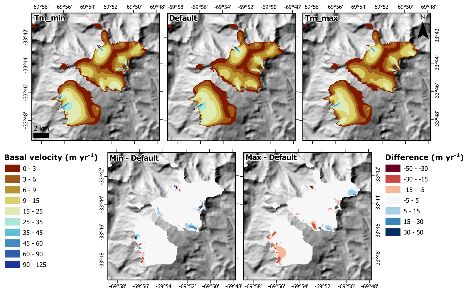
Figure 8 An example of the influence of the $W_{\mathrm{till}}^{\max }$ (Tm in figure panels) parameter on the output of ice basal velocity in the Mendoza, Maipo, and Rapel (#5) domain (Volcán Marmolejo). Remaining examples are shown in the Supplement. Increased values the Tm parameter generally sees no, or very little changes in basal ice velocities. Values that correspond to “max” and “min” parameter values are found in Table 1.

The parameters $W_{\mathrm{till}}^{\max }$ and C had minimal, to no, impact on simulated ice outputs across all domains (Fig. 7). Similar minor effects of $W_{\mathrm{till}}^{\max }$ over other valley glacier modelling efforts were reported by Candaş et al. (2020) and Žebre et al. (2021), although they saw greater sensitivity in their output than in our study due to $W_{\mathrm{till}}^{\max }$ being varied in conjunction with the till effective fraction overburden (δ). No PISM-based studies to our knowledge have assessed sensitivity to C for valley glaciers. However, variations in C have been shown to have an influence over ice sheets settings. Albrecht et al. (2020) details that increasing C from 1 to 10 mm yr⁻¹ can cause PISM to simulate an additional 11 m sea level equivalent (SLE) of meltwater from the Antarctic Ice Sheet over multiple glacial cycle timescales. This stronger influence in ice sheet settings is likely due to the greater role of subglacial hydrology in driving ice streaming, influencing basal resistance and therefore ice discharge (Kazmierczak et al., 2022; Verjans and Robel, 2024). While subglacial hydrology does not affect mountain glaciers to the same extent (Mair et al., 2002), they can affect glacier motion on diurnal time scales (Nienow et al., 2005) which would make modelling their interaction difficult. Our results indicate that these specific subglacial hydrology parameters have a limited impact on modelled ice outputs in our PISM simulations and can be removed from future sensitivity analysis. This may reflect the model resolution used here, that may limit the influence of local basal-topographic variability on sliding behaviour, or the use of the simplified representation of a non-conserving subglacial hydrology (see Sect. 3.1.2) in PISM when applied to small mountain glaciers. Alternative PISM hydrology schemes, such a steady flow or routing model, may produce stronger sensitivity in small, steep glacier catchments, allowing it to better represent the subglacial hydrology.

When ϕ was varied (Table 1), simulated ice volumes saw changes between − 40.5 % with minimum values and up to + 23.4 % with maximum values across all domains. Minimum values of ϕ led to substantial reductions in ice thickness (mean: − 24.5 %) due to increases in ice velocity (mean: + 81.9 %), while maximum ϕ values led to increases in ice thickness (mean: + 19.3 %) and reductions in ice velocities (mean: − 23.3 %) (Fig. 9). The most extreme differences were seen in the Copiapó domain, due to the region incurring the smallest glacier area, and any changes can lead to larger relative (%) changes. The values above represent the domain-mean responses. Spatially, the velocity response to variations in ϕ are not uniform. Although increasing ϕ reduced mean basal velocity across the domains, localised increases in basal velocity occurred in some areas (see Fig. 9 Phi_max). These localised increases likely reflect redistribution of ice flow where changes in basal resistance altered glacier stress balance. Similarly, while reducing ϕ increased domain-mean basal velocity, localised decreases occurred in some areas, likely due to redistribution of flow towards faster-flowing parts of the glacier system.

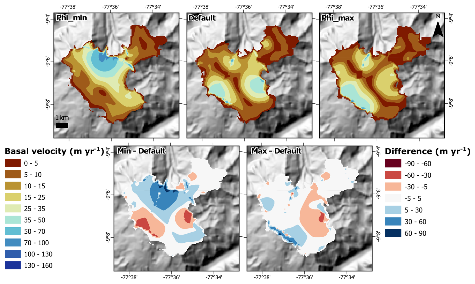
Figure 9 An example of the influence of the ϕ (Phi in Fig. panels) parameter on the output of ice basal velocity in the Santa (#1) domain (Huascaran Ice Cap). Remaining examples are shown in the Supplement. Increased values of the ϕ parameter see a domain mean reduction in basal velocities, while the opposite is seen for decreased values, however there are localised increases and decreases in velocities with higher and lower ϕ reflect localised redistribution of ice flow. Values of “max” and “min” parameter values are in Table 1.

Among the T component parameters, ϕ accounted for the greatest variance in simulated ice volume (Table 7), with a consistent influence across all domains (Fig. 7). Due to ϕ representing how resistant the subglacial sediment is to shear deformation, lower values represent wet fine sandy sediments promoting more basal sliding, while high values represent coarser dry gravels, or bedrock, reducing basal sliding (Koloski et al., 1989; Cuffey and Paterson, 2010). This therefore led to decreased domain-mean subglacial velocities, with higher values of ϕ leading to overall thicker ice (see Phi_max in Fig. 9), while lower values of ϕ increasing domain-mean velocities leading to overall thinner ice (see Phi_min in Fig. 9). The influence of ϕ over the ice basal velocities is consistent with the intuitive nature of increased values of ϕ increasing basal resistance and thus limiting basal sliding. However, the response was not uniform spatially with ice basal velocities presenting the opposite to the domain-mean pattern within localised areas (i.e., increase ϕ seeing increase localised velocities and vice versa). These are likely due to changes in the ice divides and flow regimes that can lead to subsequent changes in the ice thicknesses and ice velocity. This localised vs. domain-mean effect of the ϕ is consistent with previous studies showing that, even when using spatial uniform parameters, there can still be spatially variable basal conditions, that can strongly influence velocity structure and sliding patterns across the model domain (Gowan et al., 2023; Johnson et al., 2023). In comparison with other studies, while ϕ has not been explicitly varied in previous mountain glacier studies, to our knowledge, when modelling ice sheets ϕ is a key control on ice volume and subsequent ice dynamics (Albrecht et al., 2020; Koldtoft et al., 2021; Lowry et al., 2020). For example, lower ϕ values saw a reduction in modelled LGM volumes of the Antarctic Ice Sheet leading to accelerated retreat, whereas higher ϕ values tended to overestimate present-day ice sheet thicknesses (Albrecht et al., 2020; Lowry et al., 2020). Our findings highlight its importance in mountain glacier settings. Though a uniform ϕ was used here, it likely varies with catchment-specific geology (Bareither et al., 2008; Clarke, 2018), suggesting future studies should tune ϕ regionally to improve accuracy in ice dynamics and volume simulations.

When all T component parameters were varied between their minimum, default, and maximum values, simulated ice volume differed by up to + 40.5 % relative to the default simulations. Across all domains, ice volumes cluster into three distinct groups centred on the minimum, default, and maximum ϕ values, most clearly seen in the Copiapó domain (Fig. 7D) and the Mendoza, Maipo and Rapel (Fig. 7E) domain. While ϕ exerts dominant control over ice volumes, C and $W_{\mathrm{till}}^{\max }$ cause only minor variations within these groups. The highest volumes occurred when ϕ and other subglacial parameters were set to their maximum values {All_max}. Pearson correlations (Table 6) confirm the strong overwhelming influence of ϕ on simulated ice outputs, with an average coefficient of 0.94 across all domains. Moreover, ϕ was the only subglacial parameter with a statistically significant effect (p≤ 0.01), underscoring its primary role in controlling model outputs in PISM.

Table 6 Pearson correlation statistics for all five model domains (n= 27 simulations per domain; 135 total) showing the influence of subglacial model parameters on simulated ice volume. The final row reports the mean absolute Pearson correlation across domains and is intended only as a descriptive summary of relative parameter influence, not as a formal regional statistic. Explanation of Pearson correlation values shown in Table 4. ${}^{**}$ $=p\le$ 0.01.

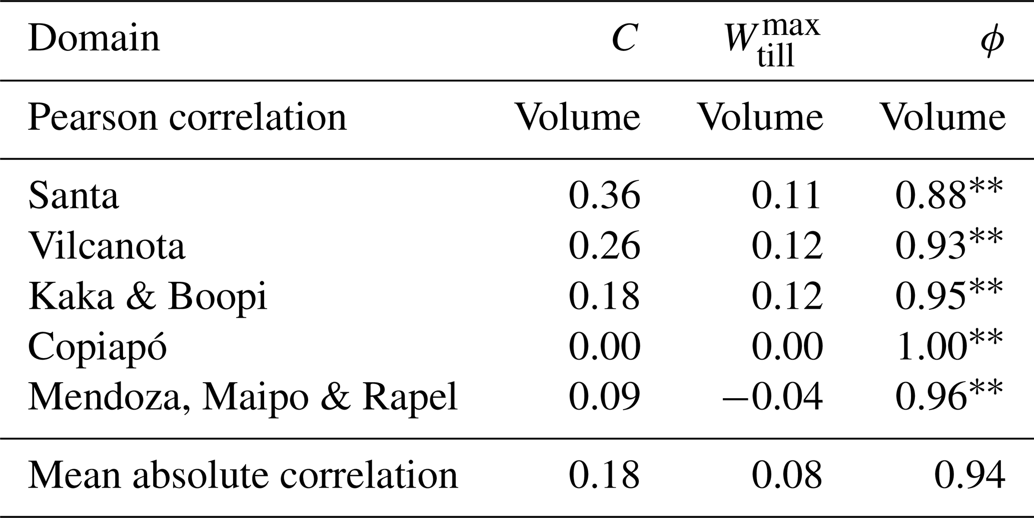
Across both univariate and multivariate parameter tests, ϕ consistently exerted the strongest influence on model outputs among the subglacial parameters. This is due to its role in the Mohr–Coulomb criterion, which governs the pseudo-plastic sliding law and modulates basal resistance (Cuffey and Paterson, 2010). Higher ϕ values increase basal resistance, slowing ice flow and leading to thicker ice, thereby raising total ice volume while having limited effect on ice extent. This relationship is reinforced by the “all max” scenario, which produced the thickest and highest volume ice across nearly all domains.

4.2.2 Sliding model parameters (S Component)

The S component tests focus on two parameters: the sliding exponent (q) and the velocity threshold (u_threshold). Summary statistics for these tests are presented in Table 7 and Fig. 10. The PISM domains of Copiapó and Mendoza, Maipo and Rapel, representing the smallest and largest glaciers respectively, display the most pronounced responses to parameter variation, with maximum ice volume changes of 44.1 % and 30.0 %, respectively.

Table 7 Sliding sensitivity analysis outputs detailing the default model simulation area and volume, and the maximum absolute percentage changes for ice volume for each domain across all the simulations when components were varied between their maximum and minimum values.

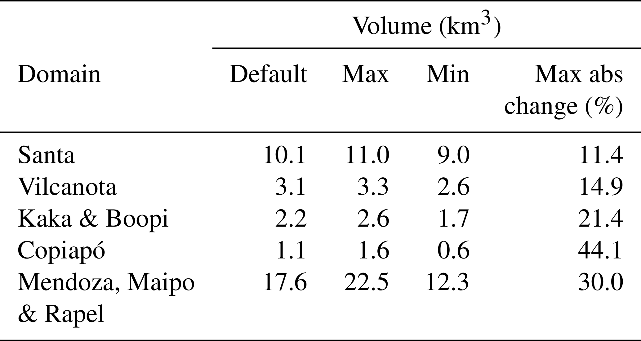
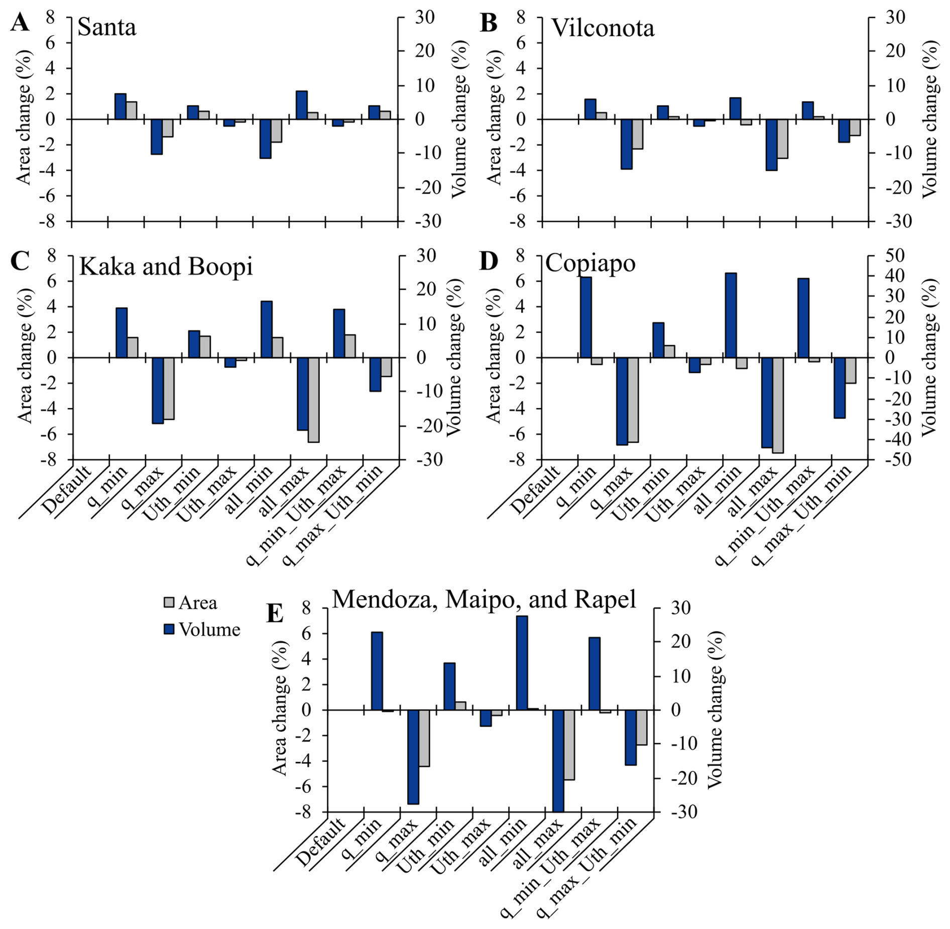
Figure 10 Sliding sensitivity analysis detailing the area (grey) and volume (blue) changes due to changing the model component parameters all together, for each of the five model domains. Blue and grey lines denote the default volume and area respectively for comparison. See Fig. 1 for domain locations. Note the change in y-axis in (D), due to larger volume changes occurring in the Copiapo catchment, the catchment with the smallest ice area.

When u_threshold was varied between its minimum and maximum values (Table 1) produced ice volume differences of + 17.1 % to − 7.2 % respectively, with an absolute average difference of 6.5 %. Across all domains minimum u_threshold saw increased ice thicknesses (mean: + 9.1 %) and basal velocities (mean: − 19.2 %) (Fig. 11). Maximum u_threshold saw reduced ice thicknesses (mean: − 3.7 %) along with increased basal ice velocities (mean: + 7.8 %).

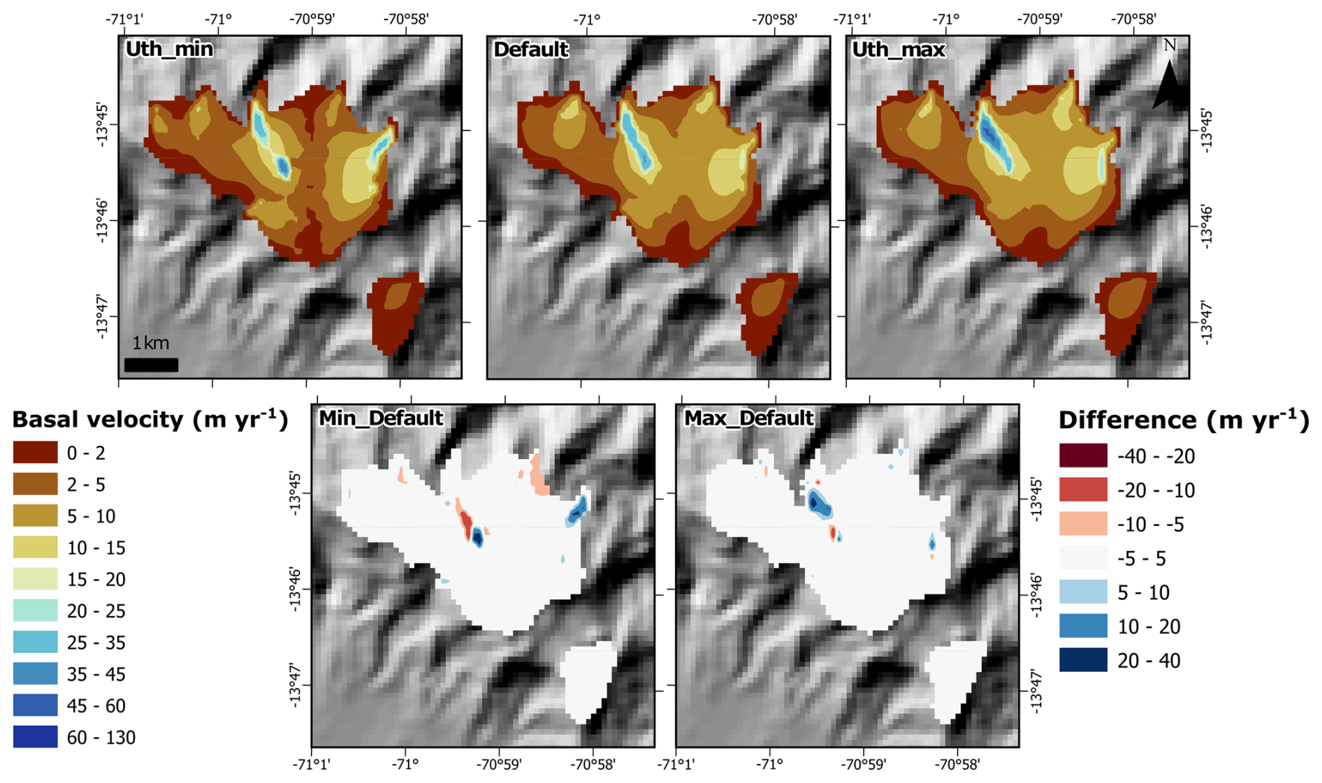
Figure 11 An example of the influence of the u_threshold (Uth in figure panel) parameter on the output of ice basal velocity in the Vilcanota (#2) domain (Quelccaya Ice Cap). Remaining examples are shown in the Supplement. An increase in the u_threshold parameter sees increased basal velocities, while the opposite is seen when values are decreased. Values that correspond to “max” and “min” parameter values are found in Table 1.

Variations of the u_threshold, which controls the onset of basal sliding, leads to when the u_threshold is set to lower values, ice flow velocities are decreased, increasing ice thickness and volume. However, while overall flow patterns remain very similar, their intensity shifts with varied u_threshold values. As can be seen in Fig. 11, with decreased u_threshold values overall mean velocities decreased, but small localised areas of increased velocities (∼ 10 to 20 m yr⁻¹) are seen where in the default run saw lower velocities occurred. When the u_threshold is increased, overall mean velocity increased, with areas of already faster flowing ice saw an increase in velocity (∼ 20 m yr⁻¹), with locations of localised slower velocities remaining the same as those in the default. This behaviour is in line with the expected behaviour described in Sect. 3.1.3, whereby increases in the u_threshold delaying the transition to Coulomb-limited sliding that facilitates faster flowing ice. Despite this influence, u_threshold is rarely tested in mountain glacier modelling, with most studies using a fixed 100 m yr⁻¹ value (Martin et al., 2022; Seguinot et al., 2014, 2018). Our results, spanning 20 to 200 m yr⁻¹, show that u_threshold meaningfully affects modelled dynamics and should be included in future sensitivity analyses.

When q was varied between its minimum and maximum values (Table 1), it produced a difference in the ice volume between + 39.6 % and − 42.3 %, with an absolute average difference of 20.4 %. The two largest differences in ice volume detailed before were all seen in the smallest domain of Copiapó (− 42.3 %), the second highest difference is seen in Mendoza, Maipo, and Rapel domain (− 27.7 %), both when q is set to its maximum value. Across all domains when q was set to its minimum, there was an increase in ice thickness (mean: + 18.9 %) and a decrease in ice velocity (mean: − 33.6 %), when set to its maximum there was a decrease in ice thickness (mean: − 21.7 % and an increase in ice velocity (mean: + 75.5 %) (Fig. 12).

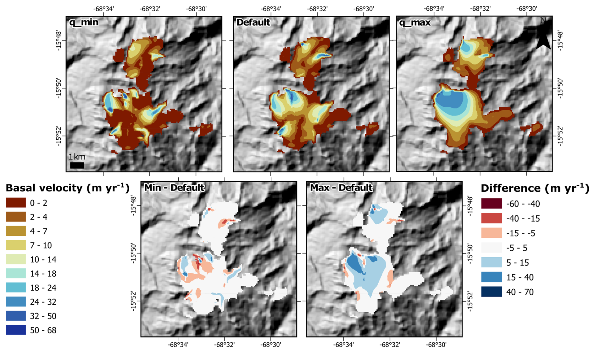
Figure 12 An example of the influence of the sliding exponent (q) parameter on the output of ice basal velocity in the Kaka & Boopi (#3) domain (Ancohuma ice caps). Remaining examples are shown in the Supplement. An increase or decrease in the q parameter sees a reorganisation of the velocities fields with more confined velocities when decreased, and more diffuse fields when increased. Values that correspond to “max” and “min” parameter values are found in Table 1.

Variations of q within PISM exert a clear influence on simulated ice dynamics, due to its role in controlling the non-linearity of the basal sliding law (Zoet and Iverson, 2020). Higher q values suppress fast-flowing regions (e.g., > 25 m yr⁻¹) but enhance sliding in slower-flowing regions, producing a more diffuse velocity field (see q_max in Fig. 12). In contrast, lower q values concentrate flow into narrow corridors, altering ice divides and increasing ice thickness in surrounding slower-flow regions by limiting basal sliding (see q_min in Fig. 12). Among PISM studies, q is the most frequently varied sliding parameter, however, this in within the context of using the default Coulomb sliding model. Using the Coulomb sliding model Candaş et al. (2020) over valley glaciers found that varying q altered ice volume by + 22.6 % at q= 0 and − 26.4 % at q= 1. In ice sheet contexts, effects are mixed with Albrecht et al. (2020) reporting lower q reduced velocity and increased Antarctic volume at the LGM by up to ± 3 m SLE. Over Greenland, Aschwanden et al. (2019) shows that the variance of q parameterization of 0.25 to 1.0 can lead to uncertainties on SLE contributions of 26 %–53 % by 2100, 5 %–38 % by 2200, and 2 %–33 % by 2300. While the Zoet and Iverson (2020) slip law has been not used by other PISM modelling studies, no study to have used the slip law within ice sheet models (e.g., CISM; van den Akker et al., 2025) varied the parameterisation of the sliding exponent extensively. Our findings here support the previous conclusion that q significantly affects modelled ice volumes, particularly in regions dominated by valley-confined dynamic flow (see Sect. 4.2.2). The results, at least for q are the first to be presented using the Zoet and Iverson (2020) slip law. We therefore recommend that future valley glacier modelling studies, especially those focused on mass change, include q in their sensitivity analyses.

When q and u_threshold are varied together between their default, minimum, and maximum values, the largest ice volume difference from the default simulation reaches − 44.1 %, observed in the Copiapo catchment (Fig. 10). Excluding this smallest domain, the maximum difference is − 30.0 % in the Mendoza, Maipo and Rapel domain. While q alone exerts the strongest influence, combining both parameters amplifies their effects {All_max}. This is particularly evident when both are set to their minimum or maximum values, resulting in greater or lesser increases in ice volume than when varied individually.

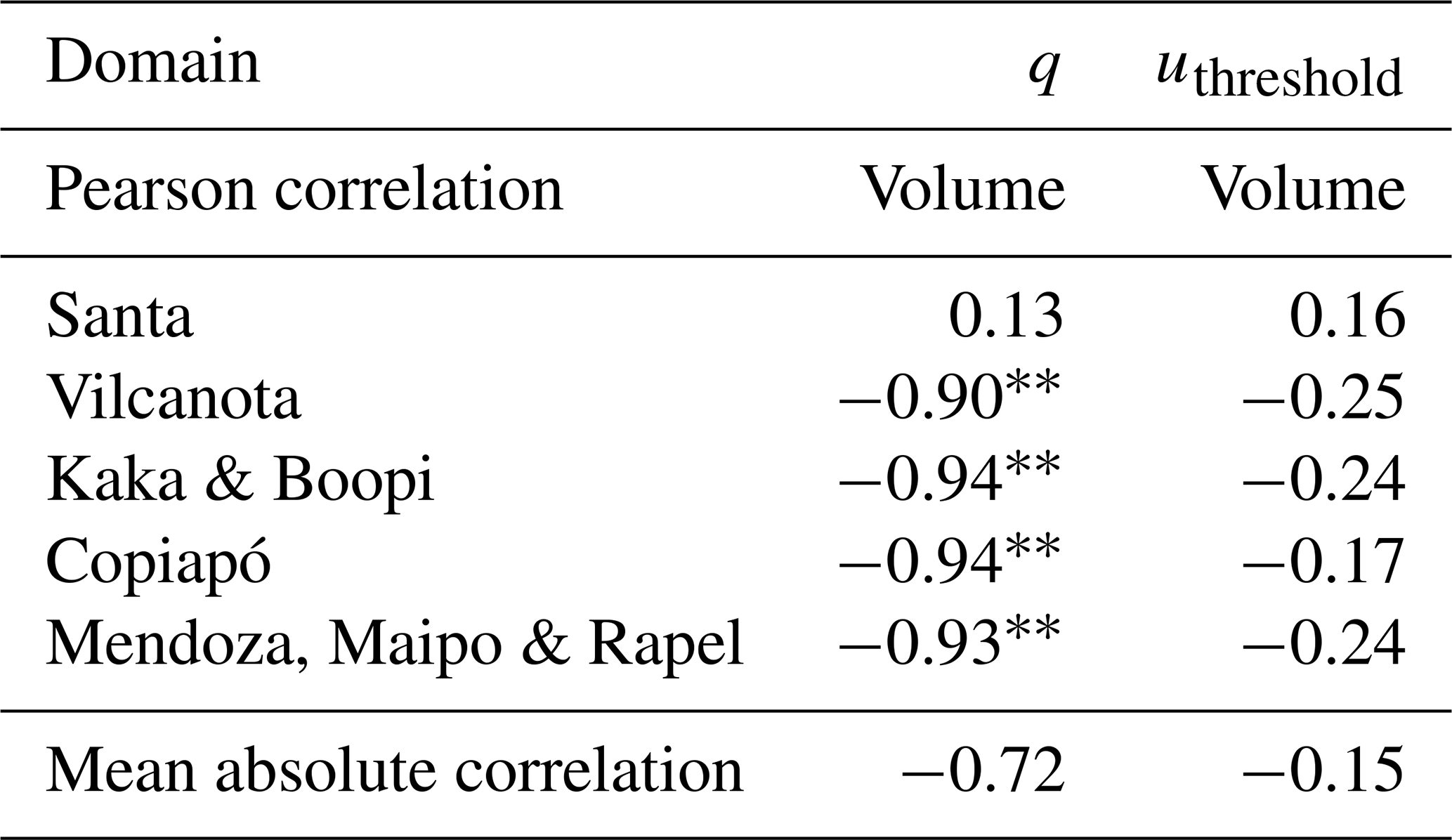
The Pearson correlation analysis (Table 8) confirms q as the dominant control on sliding-related sensitivity, with strong correlations across nearly all domains except in the Santa catchment. Although the number of combined simulations is limited, u_threshold still produces noticeable changes in simulated outputs (Fig. 11), but its influence remains secondary to q when both are varied simultaneously. This is likely because they both alter ice velocities, making it easier or more difficult for sliding to occur. This supports that these two parameters should continue to be investigated by future model efforts over mountain glaciers.

Table 8 Pearson correlation statistics for all five model domains (n= 9 simulations per domain; 45 total) showing the influence of sliding model parameters on simulated ice volume. The final row reports the mean absolute Pearson correlation across domains and is intended only as a descriptive summary of relative parameter influence, not as a formal regional statistic. Explanation of Pearson correlation values shown in Table 4. ${}^{**}$ $=p\le$ 0.01.

4.3 Implications and recommendations for future work

The findings here using PISM suggest the less influential parameters – the SIA and SSA enhancement factors (E_SIA+E_SSA), the till water decay rate (C), and the maximum till water thickness ($W_{\mathrm{till}}^{\max }$) – may be excluded from future sensitivity ensembles or parameter optimisation simulations, at least for Andean Mountain glaciers under climates close to present day. This aligns with findings from other PISM-based studies in other contexts (e.g., Albrecht et al., 2020; Candaş et al., 2020; Žebre et al., 2021), which similarly report minimal differences in modelled outputs when E_SIA, E_SSA, $W_{\mathrm{till}}^{\max }$, and C are varied within reasonable bounds. Their exclusion offers the potential to streamline future modelling efforts on their parameter perturbation selection, reducing computational demands and enabling more efficient ensemble designs. This enables researchers to allocate computational resources toward exploring more influential parameters in greater depth or across broader ranges, such as till friction angle, sliding exponent, and the velocity threshold.

Future work should examine parameters and model choice that have not been explored here. Some parameters in PISM have historically been left as “model defaults” and unchanged, based on physical assumptions or field data derived from non-valley glacier environments (or continental scale ice studies), limiting their applicability. Additionally, many parameters have not been explored in-detail within PISM for valley glaciers which, with the reduction in potential parameters to be perturbed presented here, can now be focused on. For example, future work could examine the impact of subglacial hydrology model choices, such as the difference between mass-conserving routing models and the non-conserving null model used here on valley glacier dynamics. Another example of future work can be examining the difference in the number of vertical layers within the chosen model domain. While a lower number of layers decreases computation time, and vice versa, this factor has not been studied in detail to understand how vertical grid resolution impacts basal thermal regimes, ice flow, and the overall model output over mountain glaciers.

Results from this study demonstrate that ice flow parameters influence simulated ice volume, while for ice area it is mainly unaffected. For applications related to water resources, such as runoff or meltwater estimates, understanding the internal ice physics and associated parameter sensitivities on ice volume is essential to understand how much ice (or water) remains in the future. However, studies that focus on glacier area, or are lacking robust ice volume constraints, should prioritise sensitivity analysis for climatic parameters, in particular those that effect PDD model. As shown in previous study, for transient simulations, climatic parameters such as degree day factors snow and ice exert the strongest control over both ice area and volume (e.g., Martin et al., 2022). Further, PISM has also added the new diurnal energy balance model simple (dEBM-simple) that improves upon the PDD model by accounting for melt-albedo feedback and shortwave radiation, without a significant increase in computational time (Zeitz et al., 2021). This model has only been applied in ice sheet settings but may better represent climatic interactions over mountain glaciers given its explicit consideration of radiative melting.

5 Conclusions

This study investigated the influence of internal ice flow parameters within PISM over valley glaciers across our five Andean domains (8 hydrological catchments) in South America. We examined parameters tested in previous studies, that have either identified parameters as having a large influence over, or having mixed influence, over ice model outputs, in different glacial environments. By applying these tests across multiple domains of varying sizes, we evaluated whether sensitivity differed with glacier scale. While the smallest (Copiapó) and largest (Mendoza, Maipo and Rapel) model domains, with the least and most ice respectively, exhibited the most pronounced volume differences, the overall response to parameter perturbations was relatively consistent across all domains.

Of the components assessed, the enhancement factors showed the least sensitivity, producing the least difference in ice volume. Within the subglacial component, the parameters C and $W_{\mathrm{till}}^{\max }$ saw negligible impact on modelled ice outputs. We therefore suggest that further testing of these parameters is unnecessary for similar valley glacier modelling applications in PISM, especially under climate and glacier conditions close to present day.

The sliding component parameters of the velocity threshold (u_threshold) and sliding exponent (q), exhibited moderate influence over ice volume. While both impacted ice thickness and velocity, q had the dominant influence when the sliding component parameters were perturbed together. Within the till component, the greatest overall control on simulated ice volume came from the till friction angle (ϕ). This saw the largest differences produced in ice thickness and basal velocities. This underscores the dominant role of basal conditions in valley glacier dynamics within PISM and a parameter that should see further investigation within modelling studies.

Unlike most previous PISM sensitivity studies, which have focused on ice sheets or limited mountain glacier domains, this study systematically examined the influence of internal ice dynamics on valley glaciers in the Andes. Our findings reinforce the need for detailed investigation of subglacial-related parameters, especially basal resistance (ϕ). We also detail continued support for the investigation of the sliding exponent (q), at least within the Zoet and Iverson (2020) slip law, which was recently implemented into PISM and has not been varied before this study. We also recommend that future studies explore the role of subglacial hydrology models, such as the choice between mass-conserving and non-conserving schemes, and their potential influence on modelled glacier behaviour, and just how this influence may be affected by model resolution.

This work represents the first stage in the glacier modelling workflow of the Deplete and Retreat project. The insights gained here will directly inform the design of a Latin Hypercube ensemble by eliminating parameters with negligible impact, thereby refining the efficiency and robustness of subsequent simulations. Our results can inform future sensitivity analyses and optimisation studies for glacier and ice sheet models, enabling researchers to prioritise parameters with substantial impacts on model outputs and avoid testing those with minimal influence. This efficiency can help conserve computational resources while guiding more targeted investigations into parameter effects on modelled ice outputs.