Comparing high spatial and temporal resolution snow depth measurements and modelling results in an avalanche release area

Accurate representation of snow depth distribution within avalanche release areas is critical for understanding avalanche formation and supporting operational avalanche mitigation measures. In this study, we investigate the spatial variability of snow depth in an avalanche release area using high spatial (0.5 m) and temporal (hourly) resolution measurements obtained from a low-cost terrestrial laser scanner (TLS). The TLS data provide detailed snow depth distribution maps. We analyse three selected snow accumulation events, including sub-event evolution, enabling an event- and sub-event-based analysis of snow deposition patterns.

We assess the ability of three terrain-based modelling approaches to reproduce observed snow depth patterns: the topographic position index (TPI), a wind shelter index (Sx), and a statistical preferential deposition model. The results indicate that simple topography-derived indices generally achieve the highest correlations with measured snow depths across most analysed events. The correlations reach maximum values of up to 0.57 (Spearman correlation), indicating that topographic predictors are able to partially, but not fully explain the present snow depth variability at sub-metre spatial resolution.

These findings emphasise the dominant role of local terrain in shaping snow accumulation patterns within avalanche release areas, demonstrate the value of TLS data for event-scale model evaluation, and highlight the potential to complement incomplete observations using simple terrain-based modelling approaches. The collection of additional snow depth distribution data with such high spatio-temporal resolution in different avalanche release areas would enable the development of machine learning approaches in the future. This fosters event-based avalanche forecasting by improving the spatial completeness of snow depth observations in complex terrain at slope scale.

1 Introduction

Spatial variability in snow depth is a defining characteristic of alpine snow covers and is particularly relevant in avalanche release areas, where local snow loading can strongly influence slab formation and release. Wind loading, which commonly occurs on lee slopes during or after snowfall, is a major contributor to avalanche formation, as it can form cohesive wind slabs above soft or weak layers (Schweizer et al., 2003). Accurate knowledge of the spatial snow depth distribution is therefore crucial for avalanche forecasting and risk-based decision-making, for example for the operation of remote avalanche control systems or temporary road closures.

The spatial variability of snow depth across a slope is determined by several processes. A key factor is wind, leading to preferential deposition during snowfall events from the interaction of snow particles with topography and wind (Föhn and Meister, 1983; Lehning et al., 2008). After deposition, when the wind speeds exceed the threshold friction velocity (Li and Pomeroy, 1997), it leads to substantial snow redistribution (Lehning and Fierz, 2008; Li et al., 2018) as well as to drifting snow sublimation (Groot Zwaaftink et al., 2013), resulting in substantial spatial differences in snow accumulation. The spatial snow depth patterns are strongly linked to terrain characteristics, and numerous studies have quantified these relationships across a range of spatial scales. Spatial mean snow depth and snow depth variability have been related to terrain descriptors such as elevation, slope angle, curvature, aspect, local surface roughness, terrain correlation length, and upwind sheltering angle (Winstral et al., 2002; Skaugen, 2007; Grünewald et al., 2010; Schirmer et al., 2011; Lehning et al., 2011; Grünewald et al., 2013; Melvold and Skaugen, 2013; Helbig et al., 2015; Grünewald and Lehning, 2015; Schön et al., 2015; López-Moreno et al., 2017; Skaugen and Melvold, 2019; Revuelto et al., 2020a; Helbig et al., 2021; Boardman et al., 2025). However, the strength and scale of these relationships vary depending on terrain complexity, meteorological conditions, and the spatial resolution of the observations.

Measurements in mountainous terrain are often limited to point observations and automated snow depth measurements are commonly located in flat areas (flat-field stations). However, such point-wise observations have been shown to be unrepresentative for mean snow conditions in the surrounding complex terrain (Grünewald and Lehning, 2015). This limitation is particularly relevant in avalanche terrain, where snow depth variability increases considerably as the spatial scale decreases from a few square kilometers to meter-scale areas (Melvold and Skaugen, 2013; Grünewald et al., 2013; Helbig et al., 2015). For an accurate representation of spatial snow depth variability in terrain prone to avalanches, measurements with high spatial resolution (sub-meter) are inevitable.

The most established approaches for mapping snow depth at high spatial resolution include terrestrial laser scanning TLS (Prokop, 2008; Grünewald et al., 2010; Schirmer et al., 2011; Deems et al., 2013; Adams et al., 2013; Revuelto et al., 2014; Deems et al., 2015; Voordendag et al., 2024) and aerial photogrammetry (Bühler et al., 2015; Vander Jagt et al., 2015; Nolan et al., 2015; Meyer et al., 2022; Bührle et al., 2023). These approaches require high logistical and financial effort, typically rely on suitable meteorological conditions (Bühler et al., 2016), and are thus often limited to a few acquisitions per winter season. More recently, low-cost lidar sensors have been explored for snow-related applications, including avalanche detection and validation (Kapper et al., 2023). Building on these developments, research groups have also started investigating the potential of permanently installed low-cost lidar systems for continuous snow depth monitoring (Ruttner et al., 2025a; Goelles et al., 2025).

Nevertheless, in most regions observations from avalanche release areas in real time and with high spatial resolution are not available. Even in places where for example lidar sensors are installed, it is likely that they fail to provide meaningful data during periods of fog or strong snowfall. Thus, in the absence of spatial observations or when data are missing, a modelled spatial snow depth distribution can provide valuable information.

A wide range of modelling approaches has been developed to represent spatial snow depth variability. Complex atmospheric snow-transport models explicitly resolve the interaction between wind, snow particles, and terrain, including processes such as saltation, suspension, deposition, and erosion (Liston and Sturm, 1998; Gauer, 2001; Schneiderbauer and Prokop, 2011; Vionnet et al., 2014; Gerber et al., 2017; Wang and Huang, 2017; Li et al., 2018; Hames et al., 2022; Saigger et al., 2024; Aksamit et al., 2026). Models that couple physical snow processes to detailed snowpack schemes, such as Alpine3D (Lehning et al., 2006) or SnowPappus (Baron et al., 2024), are designed for snow cover simulations that can cover large domains and are in part also in operational use. However, these approaches require substantial computational resources and comprehensive wind field data, which restricts either the spatial extent, the temporal extent, or the spatio-temporal resolution of the modelling.

To balance physical realism and computational efficiency, several models with intermediate-complexity have been proposed. These approaches simplify certain transport processes while retaining essential dynamics of wind-driven snow redistribution, enabling larger domains or longer simulation periods at manageable computational cost (Vionnet et al., 2021; Quéno et al., 2024). Lower-complexity models, such as statistical models, relate terrain and meteorological parameters to snow depth patterns (Grünewald et al., 2013; Revuelto et al., 2020b; Meloche et al., 2022; Daudt et al., 2023; Helbig et al., 2024). These data-driven methods offer attractive alternatives, but when trained on data from a single region, they risk regional overfitting (Revuelto et al., 2020b).

Despite substantial progress in observing and modelling spatial snow depth variability, important limitations remain, particularly in the steep slopes of avalanche release areas. Many existing studies focus on a basin-scale, with resolutions of 10–100 m, while investigations at sub-metre spatial resolution are rare. Furthermore, although individual snowfall events have been analysed using terrain-based parameters (Prokop et al., 2013; Schön et al., 2015), the time gaps between snowfall and measurement often span several days. During such periods, additional processes such as settlement and melt may alter the snow depth distribution, making it difficult to isolate the effect of wind-driven preferential deposition and redistribution. Previous studies scaled modelling approaches with measurements using for example blowing-snow flux measurements (Schön et al., 2018), and have demonstrated the value of lidar-derived spatial snow depth data for model evaluation and practical applications (Prokop and Procter, 2016). However, the applicability of relatively simple terrain- and wind-based models for event-scale changes in snow depth at high spatial resolution remains uncertain due to the limited availability of high spatio-temporal validation data.

In this context, we focus on low-complexity models that differ in the processes they represent and in their typical scales of application. Indices such as TPI (Weiss, 2001) and Sx (Winstral et al., 2002) provide simple descriptors of terrain characteristics that can be related to local snow redistribution patterns, whereas preferential deposition models (Helbig et al., 2024) address a different process and are usually applied at coarser resolution. In steep avalanche release terrain, where multiple processes may act simultaneously, the transferability of such approaches remains unclear. Our high spatio-temporal resolution lidar dataset allows a consistent comparison under different dominant processes.

In this study we compare observations of changes of snow depth (ΔHS) at high spatio-temporal resolution, with ΔHS derived from terrain and wind-exposure indices as well as from a statistical downscaling model for preferential deposition. We further assess the sensitivity of modelled ΔHS to different wind inputs, the use of a snow-covered instead of a snow-free DSM, and different mean precipitation inputs for scaling. Finally, we evaluate the potential of these approaches to fill spatial gaps in the measurement data caused by adverse weather conditions or terrain shadowing related to the lidar setup geometry.

2 Data

2.1 Terrestrial laser scanning (TLS) data

This study uses snow depth data from two permanent low-cost terrestrial laser scanning stations (B1 and B2) at the test site Braemabuel, in the Dischma valley near Davos, Switzerland (see Fig. 1). The observed slope represents the release area of the Wildi avalanche path, is northeast-facing, and ranges from approximately 2150 to 2250 m a.s.l., with inclinations between 30 and 45°. The terrain is characterized by heterogeneous subalpine vegetation, including grass, low shrubs, and a few small, scattered trees, as well as rocky patches.

At each of the laser scanning stations, we operate a Livox Avia lidar sensor. Jointly, these sensors cover the typical release area of the Wildi-avalanche. The lidar sensors measure at a wavelength of 905 nm which is optimal for sensing snow (Wiscombe and Warren, 1980; Prokop, 2008). We installed the sensors on 23 November 2023 and configured them to scan every hour. The specified maximum measurement range of the lidar sensors is 450 m, but in our region of interest we achieve around 150 m, due to the suboptimal measurement geometry. The data cover an area of about 14 500 m², with an average resolution of 0.1 m. Accounting for measurement accuracy, registration errors and rasterization/interpolation errors the data has an accuracy of 0.1–0.3 m. We processed the data to a gridded raster data of 0.5 m resolution. A more detailed description of the sensors, setup, data processing, and data quality is given in Ruttner et al. (2025a).

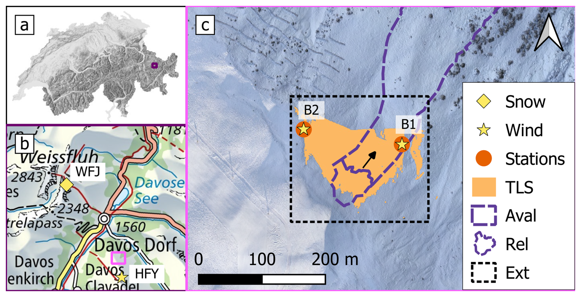
Figure 1 Overview of the study area Braemabuel (a) within in Switzerland, (b) near Davos and the snow measurement station Weissfluhjoch (WFJ) and the wind station Holfuy Braemabuel (HFY), and (c) the locations of the measurement stations (including wind measurements), the area covered by the terrestrial lidar scans (TLS), outline (Aval) and release area (Rel) of the Wildi avalanche in 2019, and the extent used for modelling changes of snow depth (Ext, 217×198 m). The arrow indicates the flow direction of the avalanche. The background image is an orthophoto derived from the photogrammetric drone flight on 12 December 2023. Map source: Federal Office of Topography.

2.2 Meteorological data

Across the approaches for modelling snow depth distribution in our study, we use wind direction, wind speed, precipitation amount and snow density data. To ensure comparability, robustness and applicability of our approaches, we primarily rely on data from numerical weather prediction models, which offer greater consistency and coverage compared to station-based measurements. Specifically, we use the Kenda-CH1 analysis data of the ICOsahedral Non-hydrostatic (ICON) modelling framework (Zängl et al., 2015) as meteorological input for all models in the main analysis, including precipitation as well as wind speed and wind direction, available on a 1.0 km grid at 10 m above ground in Switzerland. We use the hourly values of the grid cell, whose centre is closest to our study site. This choice was made intentionally to ensure a consistent basis for comparing the model approaches and to evaluate their applicability in settings where local weather stations are not available. To our knowledge, there has not been a specific validation of the ICON-derived HNWs. Given the improved score for precipitation of ICON over COSMO (Lapillonne et al., 2026), we expect that the bias in snowfall amounts is reduced compared to the −19 % found for COSMO (Magnusson et al., 2025).

In addition to the main ICON-based analysis, we use wind data from local weather stations to assess the sensitivity of model performance to the choice of wind input. Close to our test area there are three weather stations that measure, among other parameters, wind speed and wind direction: Our TLS measurement stations B1, B2 (see Fig. 1c) and the wind station HFY on top of the close-by peak (500 m horizontal, and 200 m vertical distance, see Fig. 1b). The data of the latter is accessible through the platform holfuy (Holfuy, 2025).

For the conversion between snow water equivalent and snow depth, we additionally require the density of new snow. The closest measurement station at similar altitude, where all information is available to derive snow density, is at Weissfluhjoch (WFJ), located about 5.5 km from our test site Braemabuel (see Fig. 1b). At WFJ researchers measure the height and water equivalent of new snow (HN and HNW) on a daily basis, from which we derive the density of new snow.

2.3 Terrain models

The terrain data used in this study are digital surface models (DSMs), derived from photogrammetric drone flights with a Wingtra One Gen II fixed-wing UAV using a Sony RX1R II 42 megapixel camera and Post Processing Kinematics (PPK) postitioning. We processed the photogrammetric data as described in Bühler et al. (2016), Adams et al. (2018), and Eberhard et al. (2021) using the software Agisoft Metashape Professional, Version 1.6.5. We use the DSM acquired on 18 October 2022, as snow-off reference, and one from 19 December 2023, which is a DSM of the snow-covered terrain. The DSMs have a spatial resolution of 0.1 m, and we downsample them to 0.5 m to meet the resolution of the TLS data. The accuracy of the photogrammetrically derived DSMs is not explicitly assessed in this study. Based on previous studies using comparable photogrammetric workflows, we expect a vertical accuracy in the order of 0.1 m depending on illumination, surface texture, and image geometry (Nolan et al., 2015; Vander Jagt et al., 2015; Eberhard et al., 2021).

2.4 Selected meteorological events

The TLS data available to date cover the the winter seasons 2023/2024–2025/2026. In this study we focus on the winter 2023/2024, where we identified 15 potentially interesting events with a significant amount of new snow (defined as more than 0.1 m from start to end of the event). For the selection of TLS measurement epochs, we use the number of classified ground points per scan as proxy for snowfall in the monitored area, with the assumption that less ground points, mean heavier snowfall (some epochs are missing from station B2 due to sensor outages, and some from station B1 due to the scanner being snow covered). We were looking for rather short events with TLS measurements available directly before and after, so we can assume that processes other than snowfall and wind-driven redistribution, e.g., settlement or melting, have little influence on snow depth changes during the events. Among those, we selected the events without avalanche activity but with continuous availability of locally collected meteorological data (wind sensor not frozen).

With all these criteria applied, three events stand out. We indicate them as E1, E2, and E3, and analyse them, herein. They are E1: 24 November 2023, 14:00 UTC–26 November 2023, 08:00 UTC, E2: 21 December 2023, 09:00 UTC–23 December 2023, 03:00 UTC and E3: 22 February 2024, 22:00 UTC–23 February 2024, 16:00 UTC. They are distributed over the winter season and show a variety in average wind speed. With the latter we expect the presence of different processes per event (mainly preferential deposition and snow redistribution), for which we want to specifically evaluate the models. Figure 2 gives an overview of the selected events.

Due to the varying wind speeds and directions, we further divide the events into sub-events. For this, we rely on the availability of suitable lidar data (i.e. epochs which cover more than half of the test site). According to the available lidar data and best possible consideration of wind speeds and wind direction, we use the TLS acquisitions of 25 November 2023, 02:00 and 10:00 UTC during E1 and 21 December 2023, 19:00 UTC, 22 December 2023, 03:00 and 09:00 UTC during E2 (see Fig. 2). We do not have suitable lidar scans to further sub-divide E3, therefore we use only the full event herein.

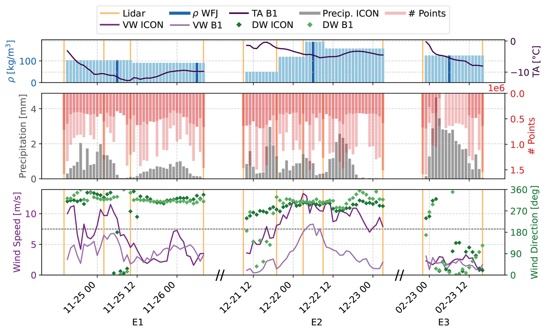
Figure 2 Meteorological conditions during the selected events. The orange vertical lines indicate the times of the lidar measurements we use in this study. The measured density of new snow ρ WFJ is shown in dark blue, and in light blue we show the interpolated values we use for each event and sub-event. TA B1 is the air temperature, measured at station B1. The precipitation values correspond to the 1 h accumulated precipitation as snowfall from the ICON dataset. The # points is the number of valid points per epoch, darker red is the point count from station B1, stacked with lighter red for the point count from station B2. For the wind direction (DW) and wind speed (VW) we show the 1 h mean values of the ICON dataset and of the measurement station B1. For orientation, we enhanced the grid line at 7.5 m s⁻¹, which is the mean threshold for snow redistribution.

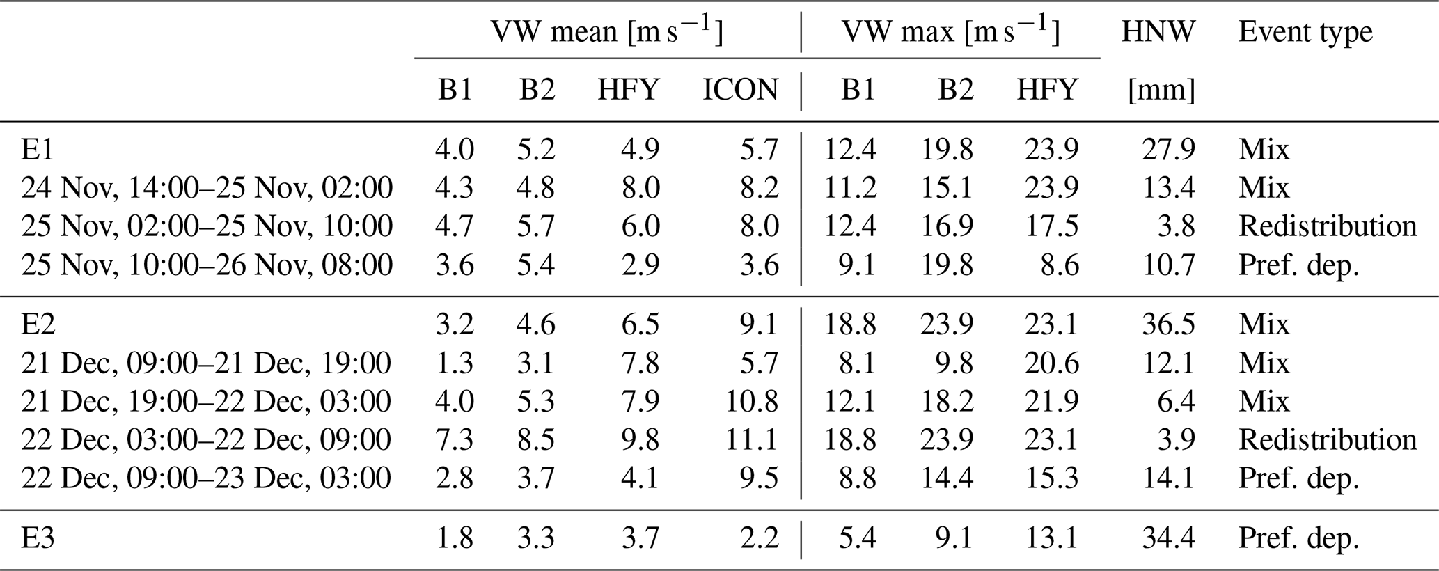
During the event in November 2023 (E1) the ICON model outputs an accumulated precipitation of 27.9 mm and average wind speeds of 5.7 m s⁻¹, mainly from north-west. At measurement station B1, which is located in the slope of interest, we recorded an average wind speed of 4.0 m s⁻¹ and gusts of maximum 11.2 m s⁻¹. Station B2, which is on the local ridge, and HFY, located at the local peak, (see Fig. 1), measured higher values (Table 1). The threshold for snow transport is 4–11 m s⁻¹ for dry snow, with an average of 7.5 m s⁻¹ for fresh snow (Li and Pomeroy, 1997). However, this threshold depends on many factors beyond wind speed, in particular on snow surface properties. Based on the locally measured wind speeds and evaluation of the differences of the TLS scans, we assume that during the event a mix of preferential deposition and snow redistribution lead to the variability of new snow depths in E1. With further dividing the event into sub-events, we assume the first hours where a mix of preferential deposition and redistribution, followed by a few hours of snow redistribution and then a period of preferential deposition in the second half of the event (see Table 1). In the event in December 2023 (E2) we retrieve an accumulated precipitation of 36.6 mm from the ICON model and an average wind speed of 9.1 m s⁻¹, from west- and north-west directions. During the first hours of the event we recorded low wind speeds of 1–3 m s⁻¹ (B1), with rather warm temperatures (while below zero). After that, the wind speeds picked up and there were a few hours with high wind speeds, on average 9.3 m s⁻¹ and gusts up to 18.8 m s⁻¹ (referring to station B1). From this we assume that there was a rather homogeneous accumulation with preferential deposition of new snow in the beginning (although due to the warmer temperatures most likely including other processes like settlement as well), which was afterwards transported and redistributed, at the same time combined with more new snow. We classify this event as well as a mixture of mainly preferential deposition and snow redistribution, with sub-events of mixed processes, redistribution and preferential deposition (also see Table 1). During the event in February 2024 (E3), the accumulated precipitation was 34.6 mm and the average wind speed reached 3.3 m s⁻¹ with great variation in wind directions, according to the ICON model. As the wind speeds recorded within the slope (on average 3.4 m s⁻¹) are below the reported threshold for snow transport, we assume that there was no snow redistribution, but mainly preferential deposition of the new snow.

Table 1 Mean and maximum wind speeds for each event and sub-event, measured at stations B1, B2, HFY and retrieved from the ICON model, as well as the accumulated water equivalent of new snow (HNW) and our event type classification.

3 Methodology

To compare the TLS measurements to the model results, we calculate snow depths with all models on the spatial extent of the rectangle “Ext” shown in Fig. 1, at 0.5 m resolution. All comparisons to TLS measured change of snow depth (ΔHS), are performed only on the pixels where TLS measurements are available (individual mask per event).

3.1 Topographic position index TPI

The topographic position index TPI (Weiss, 2001) describes the relative elevation of a point, compared to the mean elevation of the surrounding terrain, in an application-specific radius. This allows the use of TPI to indicate slope positions and landforms, such as depressions, plains or ridges and hilltops. Depending on the selected radius, different scales of topography are described (Weiss, 2001).

The TPI is calculated as follows:

$$\begin{array}{}\text{(1)}& {\text{TPI}}_j^R=z_j-{\overline{z}}_j^R\end{array}$$

where j is the index of the cell ${\mathbf{X}}_j(x_j,y_j,z_j)$ for which the TPI is evaluated, and ${\overline{z}}_j^R$ is the average elevation of all points within a circle of radius R around point X_j. For simplicity, we will subsequently omit the superscript R, herein. In our implementation we exclude a margin near the borders and represent missing values with NaN. TPI is only computed where the fraction of NaN values within the radius R is below 10 %, an empirically chosen threshold. For a DSM resolution of 0.5 m and R=10 m, this yields an effective border exclusion of approximately 7 m (see Fig. 3).

Positive values for TPI indicate ridges and hilltops, whereas negative values imply landforms such as gullies and depressions, suggesting a negative correlation with snow depths. Figure 3 (top left) shows the resulting TPI, using a radius of 10 m. In Sect. 3.4 we describe our derivation of change in snow depth ΔHS from TPI.

3.2 Wind shelter index Sx

Snow depth distribution is dependent not only on the local terrain geometry, but also on the wind direction. Snow gets eroded on the windward side, and then deposits on the leeward side of a ridge. Winstral et al. (2002) developed an indicator, whether a cell is wind exposed or wind sheltered, by evaluating the terrain elevation of a cell in relation to terrain elevations of all cells in a certain wind direction and up to a user-specified distance. Whether the elevation along the assessed wind direction is higher or lower than the elevation at the point of interest provides a basic approximation of whether it is exposed or sheltered from the wind in this direction, which we assume to be positively correlated to snow depths (see Sect. 3.4 for derivation of ΔHS from wind shelter index Sx).

The windshelter index Sx of a cell ${\mathbf{X}}_j(x_j,y_j,z_j)$ describes the maximum upward slope of all cells ${\mathbf{X}}_d(x_d,y_d,z_d)$, along an azimuth angle A, and a maximum search distance D with:

$$\begin{array}{}\text{(2)}& {\text{Sx}}_j^{A,D}=max\left[\arctan \left({\displaystyle \frac{z_d-z_j}{\sqrt{(x_d-x_j{)}^{\mathrm{2}}+(y_d-y_j{)}^{\mathrm{2}}}}}\right)\right],\end{array}$$

When taking into account a number of azimuths n_A, resulting from incrementing with a defined step size from A₁ to A₂, Sx can be extended to $\stackrel{\mathrm{‾}}{\text{Sx}}$ by taking the mean of all Sx per cell j with:

$$\begin{array}{}\text{(3)}& {\stackrel{\mathrm{‾}}{\text{Sx}}}_j^{A,D}{\mathrm{|}}_{A_{\mathrm{1}}}^{A_{\mathrm{2}}}={\displaystyle \frac{\mathrm{1}}{n_A}}\sum _{A=A_{\mathrm{1}}}^{A_{\mathrm{2}}}{\text{Sx}}_j^{A,D},\end{array}$$

We take the approach a step further and instead of equally weighting all considered wind directions in the above $\stackrel{\mathrm{‾}}{\text{Sx}}$, we compute a wind rose and calculate a weighted mean ${\stackrel{\mathrm{‾}}{\text{Sx}}}^{\mathrm{w}}$, according to the relative occurrence of the observed wind directions within azimuth bins of a specified angle width. This ensures that dominant wind directions get more weight and less frequent wind directions are taken into account, but are not over emphasised. In the remainder of the paper we use ${\stackrel{\mathrm{‾}}{\text{Sx}}}^{\mathrm{w}}$ for our analysis, but use the notation Sx, for simplicity. We calculate Sx in hourly time steps, scale each time step using the corresponding mean water equivalent of new snow $\stackrel{\mathrm{‾}}{\text{HNW}}$ from ICON, apply weighted means from 5° wind direction angular intervals, and then accumulate the results to the time intervals, as defined with the events. In Fig. 3 (top center) we show the Sx angles for an example epoch of 25 November 2023, 21:00–22:00 UTC, where the average wind direction was from 315°.

3.3 Preferential deposition from statistical snowfall downscaling PD

Helbig et al. (2024) developed a statistical snowfall downscaling scheme based on parameters derived from a comprehensive 30 m new snow database, generated using 3D atmospheric model wind simulations over synthetic topographies spanning a broad range of slope characteristics, together with a snow transport model to compute preferential deposition. This dataset describes how snowfall is non-uniformly deposited on the ground in mountainous terrain due to interactions between near-surface wind, snow particles, and topography. Processes such as snow erosion, saltation, drifting snow sublimation, and snow melt or settlement were intentionally suppressed and are therefore not represented in the PD model. The downscaled snowfall (PD), or water equivalent of new snow j ${\text{HNW}}_j^{\mathrm{PD}}$ per cell is calculated by scaling $\stackrel{\mathrm{‾}}{\text{HNW}}$ by a local downscaling factor X_dsc,j:

$$\begin{array}{}\text{(4)}& {\text{HNW}}_j^{\mathrm{PD}}=\stackrel{\mathrm{‾}}{\text{HNW}}{X}_{\mathrm{dsc},j}\end{array}$$

X_dsc,j describes primarily the correlation of preferentially deposited snowfall with local vertical wind speed w_j (with updraft on the windward side of mountains and downdraft on the lee side), in line with earlier studies reporting correlations between vertical wind speed and preferential deposition (Lehning et al., 2008; Dadic et al., 2010). Helbig et al. (2024) further showed that preferential snowfall deposition scales with the local slope parameter μ_j, which is calculated for each cell j, from its partial derivates ∂_xz and ∂_yz (${\mathit{\mu }}_j=\sqrt{\left(\right({\partial }_{\mathrm{x}}z{)}^{\mathrm{2}}+\left({\partial }_{\mathrm{y}}z{)}^{\mathrm{2}}\right)/\mathrm{2}}$). X_dsc,j is

$$\begin{array}{}\text{(5)}& \begin{array}{rl}{X}_{\mathrm{dsc},j}(w_j,{\mathit{\mu }}_j)& =\text{erfc}\left(a{w}_j\right(w_j+\left|w_j\right|){)}^b\\ & \cdot (\mathrm{1}-c{w}_j+d{w}_j^{\mathrm{3}})(\mathrm{1}+e{\mathit{\mu }}_j^f),\end{array}\end{array}$$

with the following constant values for a to f: a=0.4825, b=0.03418, c=0.592003, d=0.004452, e=0.24714 and f=2.24223. X_dsc,j requires local vertical wind speed w. When spatially fine-scale w is unavailable, as in our case, Helbig et al. (2024) introduced a statistically downscaled vertical wind speed w_dsc,j for use in Eq. (5) (the “aspect scheme”). w_dsc,j is obtained by scaling the spatially averaged horizontal wind speed $\stackrel{\mathrm{‾}}{v_{\mathrm{h}}}$ with the local downscaling factor $Y_{\mathrm{dsc},j}^{\mathrm{aspect}}$:

$$\begin{array}{}\text{(6)}& w_{\mathrm{dsc},j}=\stackrel{\mathrm{‾}}{v_{\mathrm{h}}}{Y}_{\mathrm{dsc},j}^{\mathrm{aspect}}(\mathrm{\Delta }{\mathit{\psi }}_j,{\mathit{\mu }}_j).\end{array}$$

$Y_{\mathrm{dsc},j}^{\mathrm{aspect}}$ is a function of μ_j and the local terrain aspect parameter Δψ_j, defined as the local terrain aspect angle ψ_j relative to the low-resolution wind direction wd. $Y_{\mathrm{dsc},j}^{\mathrm{aspect}}$ was derived from the 3D wind simulation dataset over synthetic topographies:

$$\begin{array}{}\text{(7)}& Y_{\mathrm{dsc}}^{\mathrm{aspect}}(\mathrm{\Delta }\mathit{\psi },\mathit{\mu })=\left[(a^{\prime }-b^{\prime }(\mathrm{\Delta }\mathit{\psi })+c^{\prime }\text{erf}(d^{\prime }\left(\mathrm{\Delta }\mathit{\psi }\right))\right](e^{\prime }+{\mathit{\mu }}^{f^{\prime }}),\end{array}$$

with constant parameters $a^{\prime }=-\mathrm{0.087122}$, $b^{\prime }=\mathrm{0.4788}$, $c^{\prime }=\mathrm{2.068}$, $d^{\prime }=\mathrm{0.6298}$, $e^{\prime }=-\mathrm{0.046577}$ and $f^{\prime }=\mathrm{0.72451}$. w_dsc,j requires $\stackrel{\mathrm{‾}}{v_{\mathrm{h}}}$, which we do not have available. We use a subgrid parametrization for the spatial mean horizontal wind speed $v_{{\mathrm{h}}_{\mathrm{sgp}}}$, parametrizing the unresolved drag over topography by scaling low resolution horizontal wind speed v_h with the subgrid sky view factor $F_{\mathrm{sky},\mathrm{sbg}}(L/\mathit{\xi },\mathit{\mu })$ (Helbig et al., 2017):

$$\begin{array}{}\text{(8)}& \stackrel{\mathrm{‾}}{v_{\mathrm{h}}}=v_{{\mathrm{h}}_{\mathrm{sgp}}}=v_{\mathrm{h}}{F}_{\mathrm{sky},\mathrm{sbg}}(L/\mathit{\xi },\mathit{\mu }).\end{array}$$

$F_{\mathrm{sky},\mathrm{sbg}}(L/\mathit{\xi },\mathit{\mu })$ is parameterized as in Helbig and Löwe (2014) and relies on domain size L, domain mean slope parameter $\stackrel{\mathrm{‾}}{\mathit{\mu }}$ and terrain correlation length ξ in the domain. For further information on the PD model we refer to Helbig et al. (2024).

We calculated the HNW distribution based on PD on the same snow-off DSM as TPI and Sx, and calculate each event in 1 h time steps. Due to the locations of the measurement stations B1 and B2 we omit the sky view factor $F_{\mathrm{sky},\mathrm{sbg}}(L/\mathit{\xi },\mathit{\mu })$, when using these data as model input. Consistent with the PD model development database, grid cells with slopes exceeding 60° were excluded from the analysis and set to NaN. The final HNWs are the accumulation of the fine-scale precipitation per computation step. We convert HNW PD to HN PD using Eq. (11) adapted with ${\text{HNW}}_{j,E}^{\mathrm{PD}}$. In Fig. 3 top right we show an example epoch of the terrain scaling parameter X_dsc,j (Eq. 5), and scaled to HNW in the bottom row. For consistency with the TPI- and Sx-based results, we use the notation ΔHSW and ΔHS in the following, although the PD model is intended to describe only the accumulation of new snow and therefore corresponds more directly to HNW, i.e. positive ΔHSW.

3.4 Scaling of TPI and Sx to snow depth

The model approaches introduced above yield different output variables and units. While the PD model directly provides spatially distributed new snow amounts, the indices TPI and Sx are not directly comparable to snow depth change ΔHS and therefore require an additional scaling step.

We take a mean water equivalent of new snow per cell $\stackrel{\mathrm{‾}}{\text{HNW}}$ and determine a factor, depending on TPI or Sx, to increase or decrease the amount of HNW relative to the mean value. In our study we use the same value of $\stackrel{\mathrm{‾}}{\text{HNW}}$ for each cell, which is the value of the closest ICON cell. Based on Winstral and Marks (2002), MeteoIO (Bavay and Egger, 2014) and Helbig et al. (2024) we determine HNW of a cell with index j, depending on its Sx value, which we scale by the mean μ and standard deviation σ (over all grid cells), with:

$$\begin{array}{}\text{(9)}& {\text{HNW}}_j^{\mathrm{Sx}}=\left\{\begin{array}{ll}\stackrel{\mathrm{‾}}{\text{HNW}}\left(\mathrm{1}-\left|\frac{{\text{Sx}}_j}{{\mathit{\mu }}_{\mathrm{Sx}}-{\mathit{\sigma }}_{\mathrm{Sx}}}\right|\right)& \mathrm{if}{\text{Sx}}_j<\mathrm{0}\\ \stackrel{\mathrm{‾}}{\text{HNW}}\left(\mathrm{1}+\mathit{\alpha }\frac{{\text{Sx}}_j}{{\mathit{\mu }}_{\mathrm{Sx}}+{\mathit{\sigma }}_{\mathrm{Sx}}}\right)& \mathrm{if}{\text{Sx}}_j>\mathrm{0}\\ \mathrm{with}\mathit{\alpha }=\frac{{\sum }_{j:{\mathrm{Sx}}_j<\mathrm{0}}\mathrm{|}\frac{{\text{Sx}}_j}{{\mathit{\mu }}_{\mathrm{Sx}}-{\mathit{\sigma }}_{\mathrm{Sx}}}\mathrm{|}}{{\sum }_{j:{\mathrm{Sx}}_j>\mathrm{0}}\frac{{\text{Sx}}_j}{{\mathit{\mu }}_{\mathrm{Sx}}+{\mathit{\sigma }}_{\mathrm{Sx}}}}\end{array}\right.\end{array}$$

In the above mentioned references each cell of Sx is scaled by the Sx domain minimum (if Sx <0) or maximum (if Sx >0). We found the minimum and maximum to be very sensitive to the extent of the evaluated area, and therefore apply a scaling by mean and standard deviation in this study.

We introduce the same principle for TPI, but we assume that areas with TPI>0 are depleted and TPI<0 are enriched (relative to $\stackrel{\mathrm{‾}}{\text{HNW}}$):

$$\begin{array}{}\text{(10)}& {\text{HNW}}_j^{\mathrm{TPI}}=\left\{\begin{array}{ll}\stackrel{\mathrm{‾}}{\text{HNW}}\left(\mathrm{1}-\frac{{\text{TPI}}_j}{{\mathit{\mu }}_{\mathrm{TPI}}+{\mathit{\sigma }}_{\mathrm{TPI}}}\right)& \mathrm{if}{\text{TPI}}_j>\mathrm{0}\\ \stackrel{\mathrm{‾}}{\text{HNW}}\left(\mathrm{1}+\mathit{\alpha }\left|\frac{{\text{TPI}}_j}{{\mathit{\mu }}_{\mathrm{TPI}}-{\mathit{\sigma }}_{\mathrm{TPI}}}\right|\right)& \mathrm{if}{\text{TPI}}_j<\mathrm{0}\\ \mathrm{with}\mathit{\alpha }=\frac{{\sum }_{j:{\text{TPI}}_j>\mathrm{0}}\frac{{\text{TPI}}_j}{{\mathit{\mu }}_{\mathrm{TPI}}+{\mathit{\sigma }}_{\mathrm{TPI}}}}{{\sum }_{j:{\mathrm{TPI}}_j<\mathrm{0}}\left|\frac{{\text{TPI}}_j}{{\mathit{\mu }}_{\mathrm{TPI}}-{\mathit{\sigma }}_{\mathrm{TPI}}}\right|}\end{array}\right.\end{array}$$

We convert HNW to height of new snow HN, by using the temporal mean snow density $\stackrel{\mathrm{‾}}{\mathit{\rho }}$ for each event E = {E1, E2, E3} obtained from the WFJ observations (Fig. 1), which we assume to be constant over the evaluated area. The computed HN per pixel j and event E, derived from Sx, is therefore calculated with:

$$\begin{array}{}\text{(11)}& {\text{HN}}_{j,E}^{\mathrm{Sx}}={\text{HNW}}_{j,E}^{\mathrm{Sx}}/\stackrel{\mathrm{‾}}{{\mathit{\rho }}_E}\end{array}$$

The same equation holds for ${\text{HN}}_{j,E}^{\mathrm{TPI}}$, but using TPI to calculate ${\text{HNW}}_{j,E}^{\mathrm{TPI}}$ and for ${\text{HN}}_{j,E}^{\mathrm{PD}}$ with ${\text{HNW}}_{j,E}^{\mathrm{PD}}$.

Strictly speaking, the results of the scaling by mean and standard deviation are not HNW, since the values can become negative. We therefore refer to these model outputs as snow depth change ΔHS and, in water equivalent, ΔHSW. In the bottom row of Fig. 3 we show all scaled terrain parameters for an example epoch on 25 November 2023, 21:00–22:00 UTC, using a $\stackrel{\mathrm{‾}}{\text{HNW}}$ of 0.85 mm.

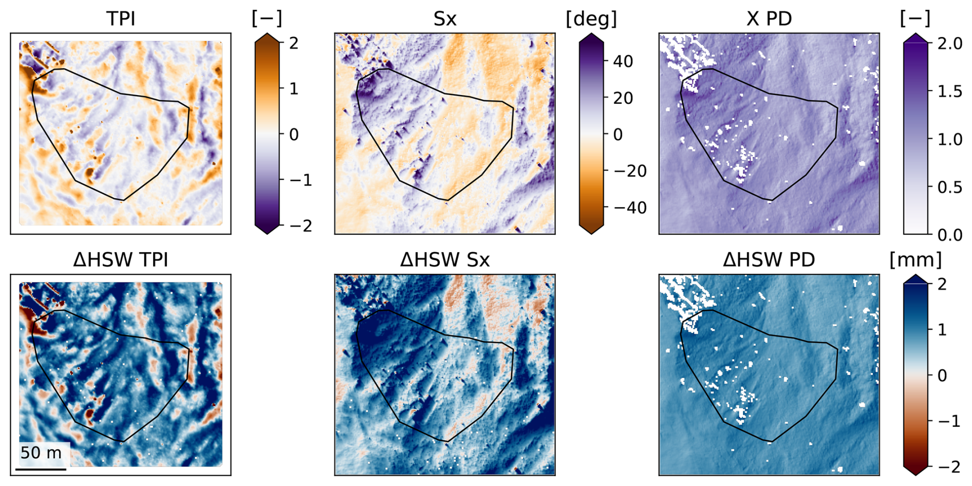
Figure 3 Upper row: terrain scaling parameters for the example epoch of 25 November 2023, 21:00–22:00 UTC. Lower row: terrain parameters scaled to ΔHSW (change in snow water equivalent), using Eqs. (10), (9), and (4). The TPI is calculated with R=10 m and for Sx we use D=8 m, a mean wind speed of 5.2 m s⁻¹ and a wind direction of 315°. The lower row is scaled with a $\stackrel{\mathrm{‾}}{\text{HNW}}$ (ICON) of 0.85 mm. X PD (upper row) corresponds to X_dsc,j in Eq. (5). The extent of the figures correspond to the outline Ext in Fig. 1. For TPI we cropped a margin of about 7 m (see Sect. 3.1). For orientation, we plot the approximate outline of the TLS data as black polygon.

4 Results

4.1 Measurements of snow depth changes

We compute our reference for change of snow depths ΔHS, by subtracting the DSM at the start of an event, from the the DSM at the end of the event, using the DSMs derived from TLS measurements. Figure 4 shows ΔHS for the three selected main events and their sub-events. In the first event (E1) we recorded a mean increase in snow depth of 0.53 m, with a standard deviation over the measured area of 0.27 m in a time of 42 h. The spatial distribution of new snow is varying, from up to 1.5 m snow accumulation in some areas to up to 0.15 m decrease in others. After the event of December 2023 (E2), we measured a mean increase in snow depth of 0.31 m, with a standard deviation of 0.23 m. The distribution pattern of snow depths is similar to E1. We find accumulations and depletions in similar areas, in both cases the prevailing wind direction during the event was north-west. The maximum accumulation of new snow is of a similar magnitude, but larger decreases occur. Several areas show a decrease in snow depth up to around −0.45 m, compared to before the event. In the last event of February 2024 (E3) the measured mean increase in snow depth is 0.37 m, with a standard deviation of 0.11 m. Due to the overall low wind speed during the event, we measured a rather homogeneous distribution of accumulated new snow without depletions.

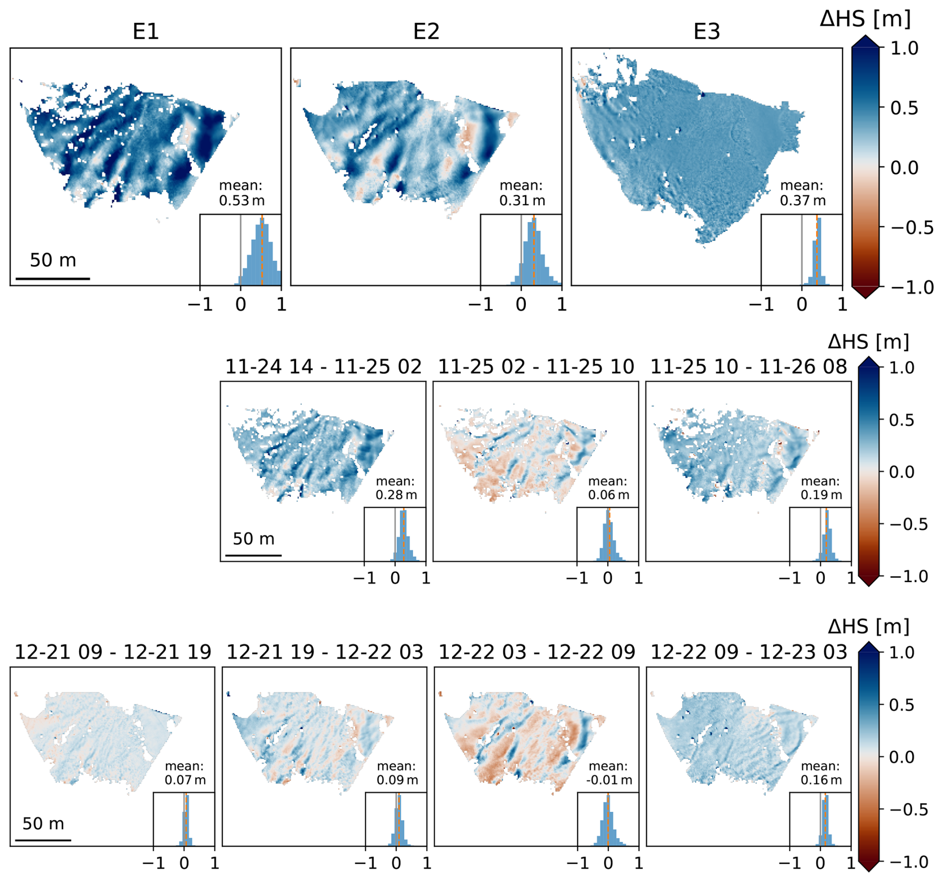
Figure 4 Measured change of snow depth ΔHS, calculated as the difference between the DSMs as “after minus before” the snowfall events. The top row shows the main snowfall events E1, E2, and E3. The middle row shows the sub-events of E1 (November 2023), and the bottom row the sub-events of E2 (December 2023). Blue colours correspond to an increase of snow depth, and red colours to a decrease.

4.2 Modelling snow depth distribution

This section first presents the parameter selection for TPI and Sx, followed by the resulting modelled snow depth distributions for the presented events.

4.2.1 Parameter selection for TPI and Sx

We calculated the indices Sx and TPI on the summer DSM. Since the TPI radius R and the Sx maximum search distance D control the spatial scale represented by the indices, we tested a range of values and evaluated their Spearman correlation with the measured snow depth change ΔHS for the events E1, E2, and E3 (Fig. 5). The optimal parameter values vary between events. For the subsequent analysis we choose R=10 m for TPI and D=8 m for Sx, and use it for all computations.

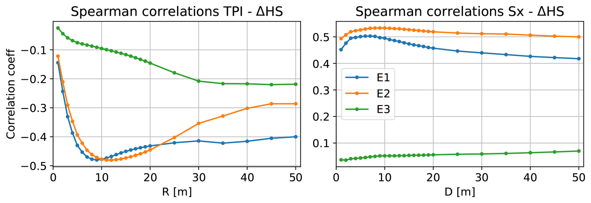
Figure 5 Spearman correlations between measured change of snow depth ΔHS (for E1, E2 and E3) and TPI and Sx, with varying radii R for TPI (left) and maximum search distance D for Sx (right).

4.2.2 Model results

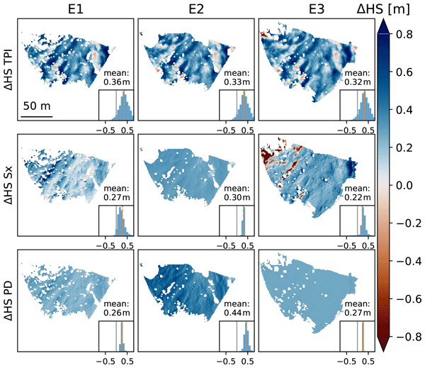
Figure 6 shows maps of the model results for the main events, and Fig. 7 shows an overview of the model results for all events and sub-events as probability density function. All results are masked by the pixels that are available from the TLS measurements. The spatial patterns of ΔHS TPI do not vary between the events, since TPI does only depend on the terrain and selected radius. In ΔHS Sx the spatial variations are different in each event, due to different wind directions. The PD model takes not only wind direction, but also wind speed into account. The difference between ΔHS Sx and ΔHS PD are for example clearly visible in E3. ΔHS Sx accumulates the distributed $\stackrel{\mathrm{‾}}{\text{HNW}}$ of each epoch of wind directions with no further scaling, resulting in large variations of snow depth distribution, where there is almost no variation resulting from the PD model.

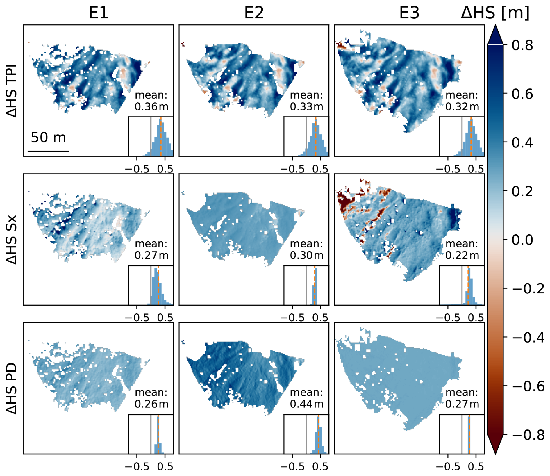
Figure 6 Spatial patterns of modelled ΔHS. The results are masked by the spatial availability of TLS measurements. The grey line in the histogram corresponds to 0.0, and the orange dashed line shows the mean value.

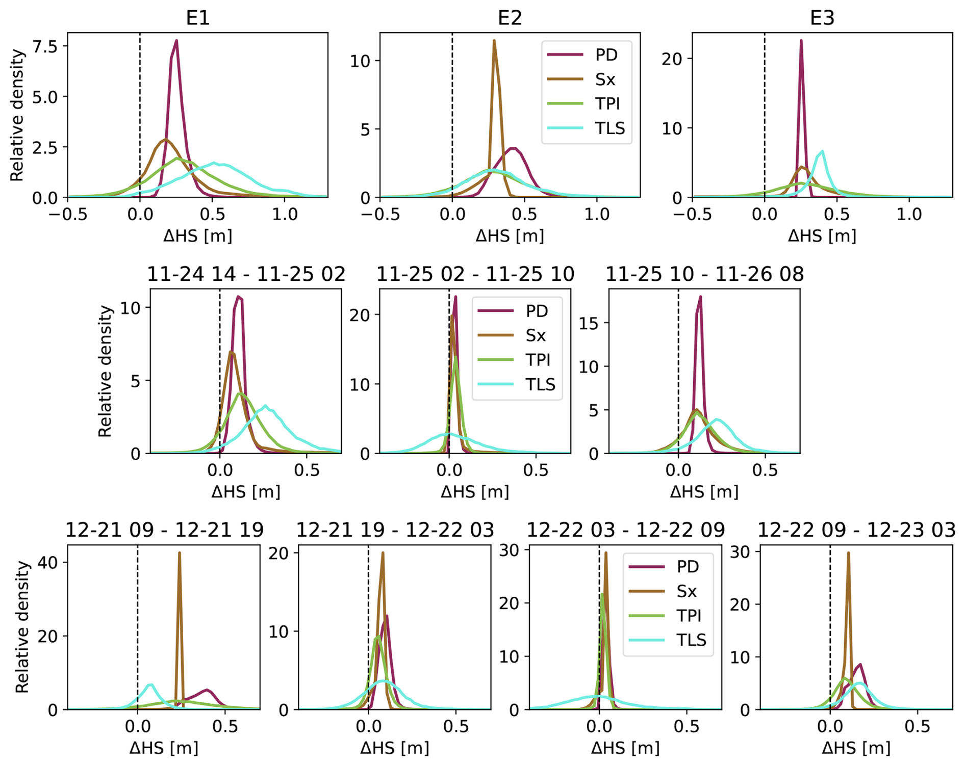
Figure 7 Probability density functions of measured and modelled ΔHS for all events and sub-events. The middle row shows the sub-events of E1 (November 2023), and the bottom row the sub-events of E2 (December 2023). The legend entries PD, Sx and TPI refer to the modelled ΔHS, we use the shorter labels for better readability of the figure.

4.3 Model evaluation

In Fig. 8 we show the differences between the measured and the modelled ΔHS. Generally, the mean differences indicate an underestimation of modelled ΔHS, compared to ΔHS TLS, with exception of the TPI and PD model in E2. The error patterns are similar in the models for E1 and E2, underestimating areas with large, positive ΔHS, and overestimating areas with small, or negative ΔHS (see insets in Fig. 8). This suggests that the main spatial structures are captured similar to the measured ΔHS, while the amplitude of the spatial variability is underestimated. In the case of E3, both ΔHS TPI and ΔHS Sx show large residual distributions, whereas ΔHS PD yields smaller and more homogeneous residuals, indicating a better agreement with the observed, spatially rather uniform snow depth distribution.

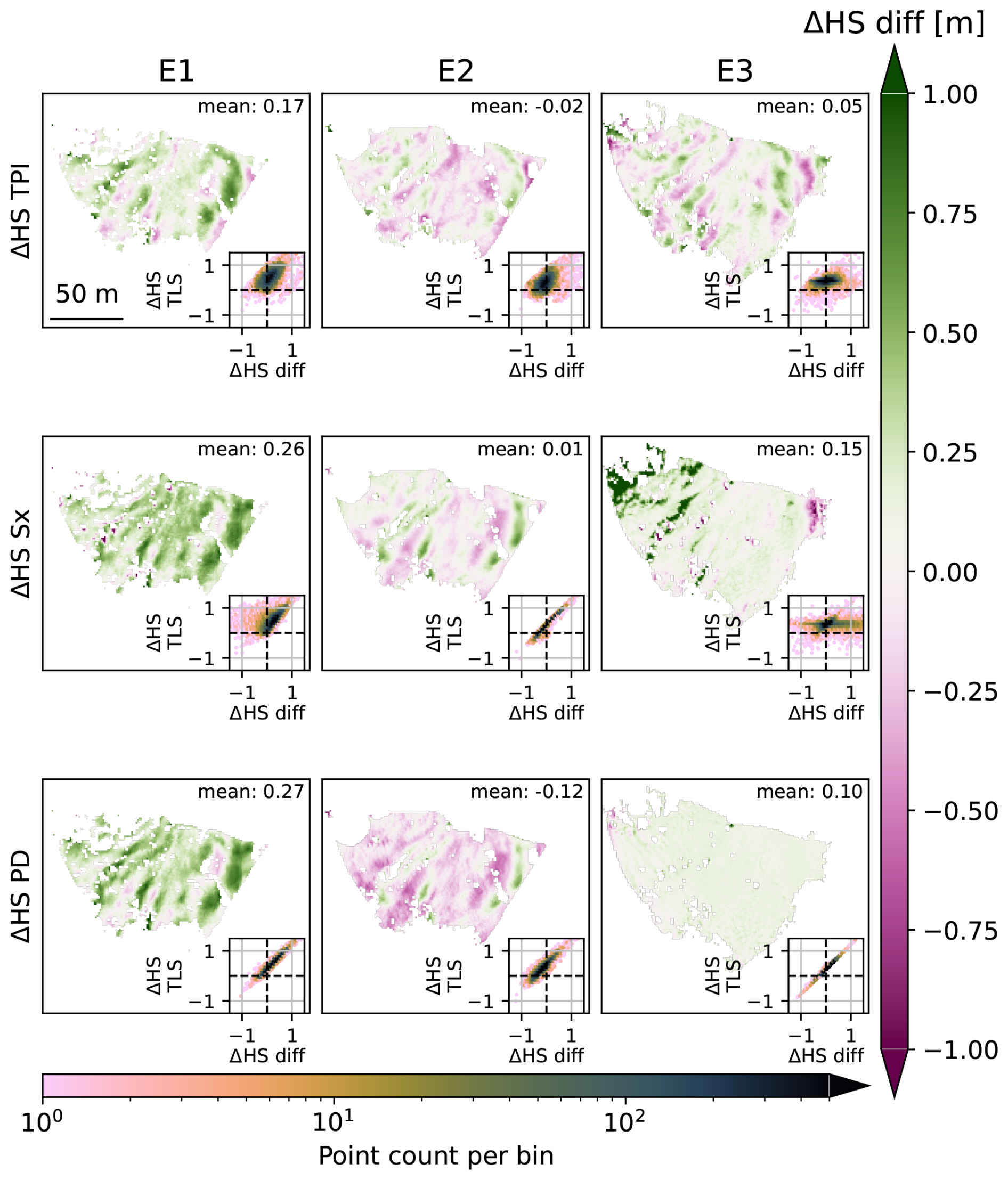
Figure 8 Differences of measured and modelled ΔHS. Positive values (green colours) indicate an underestimation of the modelled ΔHS, whereas negative values (pink) mean an overestimation of the modelled ΔHS. The mean value shown at the top right of each subplot is the mean of the residuals. The insets show hexbin plots of the residuals ΔHS diff as a function of measured ΔHS TLS, giving an indication on the dependence of the residuals on the observed snow depth change.

Figure 9 shows a comparison of the measured ΔHSs by TLS and modeled ΔHSs, using TPI, Sx and PD as scatter plots, with their Pearson and Spearman correlations coefficients (scatter plots for the sub-events are shown in Figs. A1 and A2). The highest correlations per event are achieved by the snow depths derived from the terrain indices TPI and Sx. The spatial correlations in E3 are very low for all methods. We point out the narrow distributions of ΔHS Sx in E2 and ΔHS PD in E3. The ΔHS Sx distribution is influenced by the ratio of wind exposed to wind sheltered areas, while the ΔHS PD distribution shows minimal variation in snow depths due to the low wind speeds during E3 and partially opposing wind directions during the event, which can even out the distribution of ΔHS. Overall the correlations are moderate, with a generally higher value for the Spearman correlation, compared to Pearson. This suggests that there is no purely linear correlation.

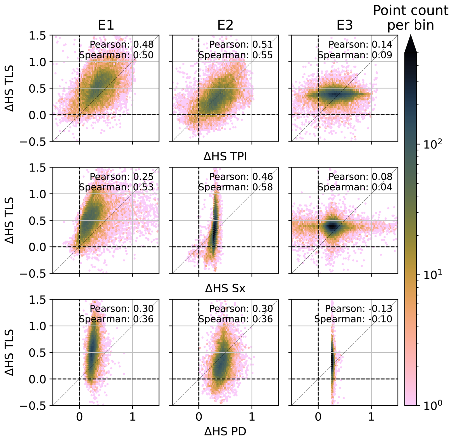
Figure 9 Scatter plots and Pearson and Spearman correlation coefficients of measured vs. modelled ΔHS. Darker colours indicate a higher count per bin.

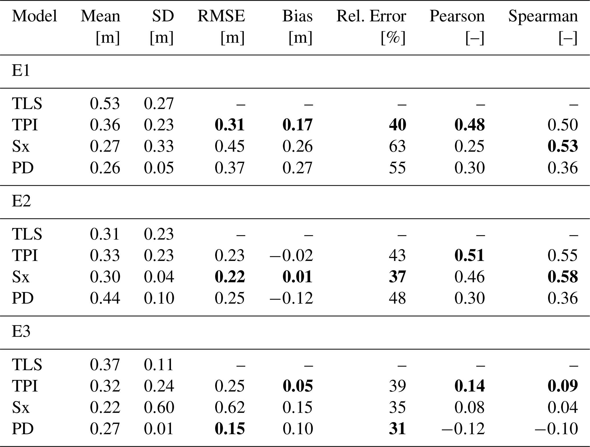
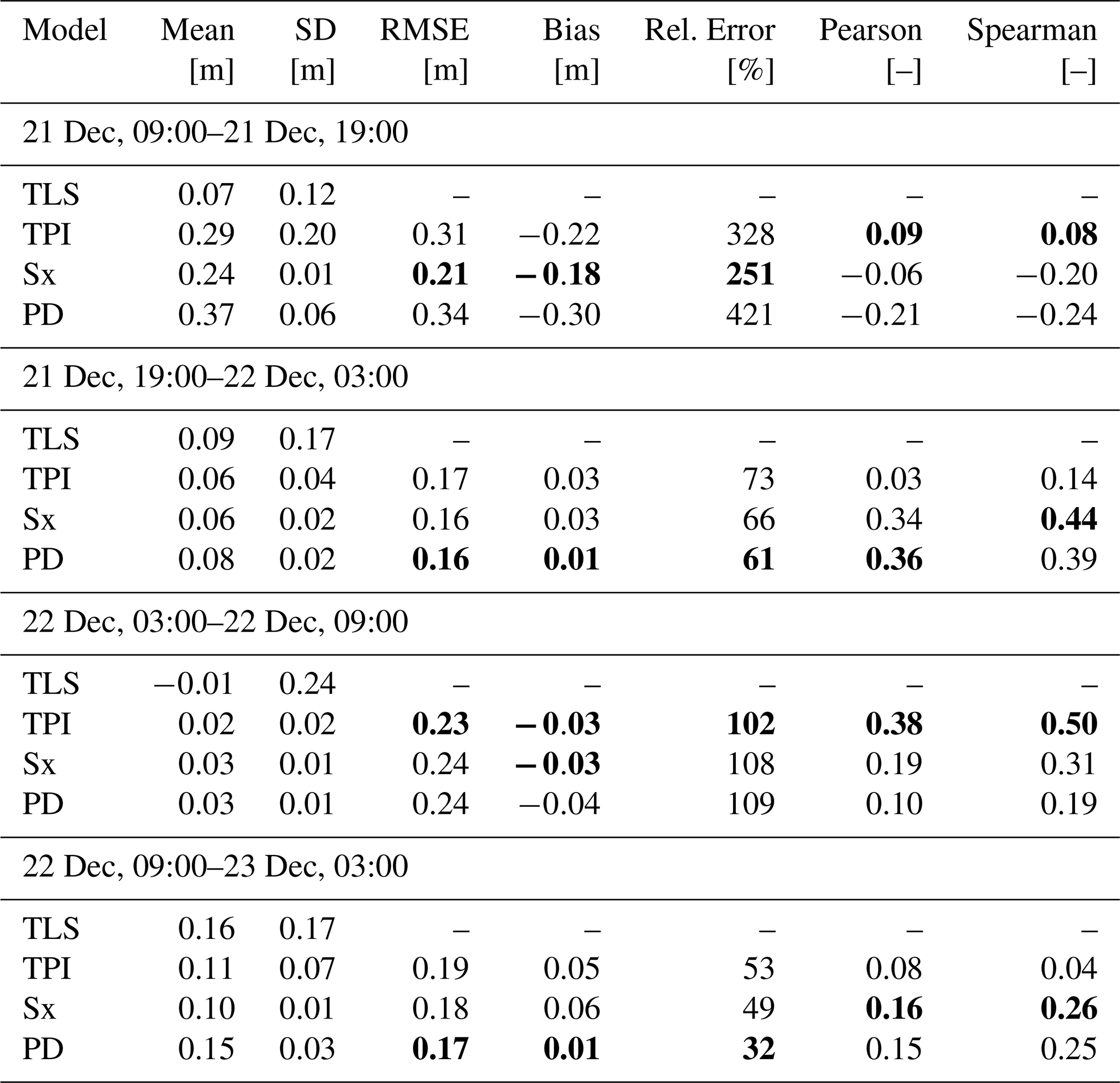
In Table 2 we summarize all performance metrics of the models, compared to the measurements. The metrics for the sub-events are in the appendix (Tables A1 and A2).

Table 2 Performance measures for different models and meteorological events. As bias we calculated the mean of the differences between the TLS measurements and the model (see also Fig. 8), and the relative error refers to the median of relative errors. The best values per model are marked in bold numbers.

5 Discussion

5.1 Sensitivity to input data and model parameters

5.1.1 Wind input

Wind plays an essential role in the pattern of snow depth distribution and many snow depth distribution models highly depend on the quality of wind field modelling. Also simple approaches, such as the wind shelter index Sx rely on the wind direction, while both wind direction and wind speeds can vary significantly within short distances in complex terrain. For slope-scale applications such as avalanche forecasting, wind stations are often located at ridges, because they best capture the incoming flow responsible for snow transport into adjacent slopes.

In our measurement setup we have several wind measurements, each at a different topographic position. One station is located within the slope of release (B1), about 150 vertical meters below the local ridge line. The other station of our main test setup is installed on top of the monitored slope, on the local ridge (B2). Furthermore, we use the data of a station located on the mountain top of Braemabuehl (HFY). All stations are within a radius of about 700 m. This gives the possibility to assess the impact of different measurement locations. In Fig. 10 we show selected metrics for the PD and Sx model, with different data for wind input (speed and direction). For the mean and standard deviations we additionally show the values derived from the TLS measurements and the ICON model. In the Appendix (Fig. A3) we include an overview of the wind speed and direction data, for each evaluated event. The variations of mean ΔHS PD are higher than for ΔHS Sx, as the PD model is also dependent on distributed wind speed, which is not considered in ΔHS Sx. The much higher standard deviations of ΔHS Sx in E3 stand out in this comparison. We attribute this to the applied scaling algorithm, which is currently not sensitive to wind speed. Among other things, we see a scaling more adaptive to wind speeds as an opportunity for improvement.

There is no clear trend regarding the proximity of the wind station, it rather depends on the representativeness of the local wind patterns. For example, station B2 is very close to the evaluated slope, but the modelled results have often a higher correlation when using the wind data from ICON. With wind data from station B1 the correlations of the modelled and measured snow depths are mostly higher than the other wind inputs. These findings emphasize the importance of carefully selecting wind stations based on local wind patterns rather than just geographical proximity when planning and operating a monitoring system.

At the same time, in many regions the measurement network is less dense than around our test site and local wind measurements are sparse or not existing. Even where wind stations exist, measurements may be affected by data gaps or sensor failures, for example due to icing during harsh weather conditions that are particularly relevant for snow redistribution processes. In this context, gridded meteorological models like ICON present a promising alternative, as they can provide consistent, high-resolution data in regions with limited or no measurement stations. However, the performance of ΔHS modelling with such data still depends on how well the gridded fields capture the local slope-scale wind patterns. Our results show that gridded wind data can perform comparably to nearby mountain weather stations.

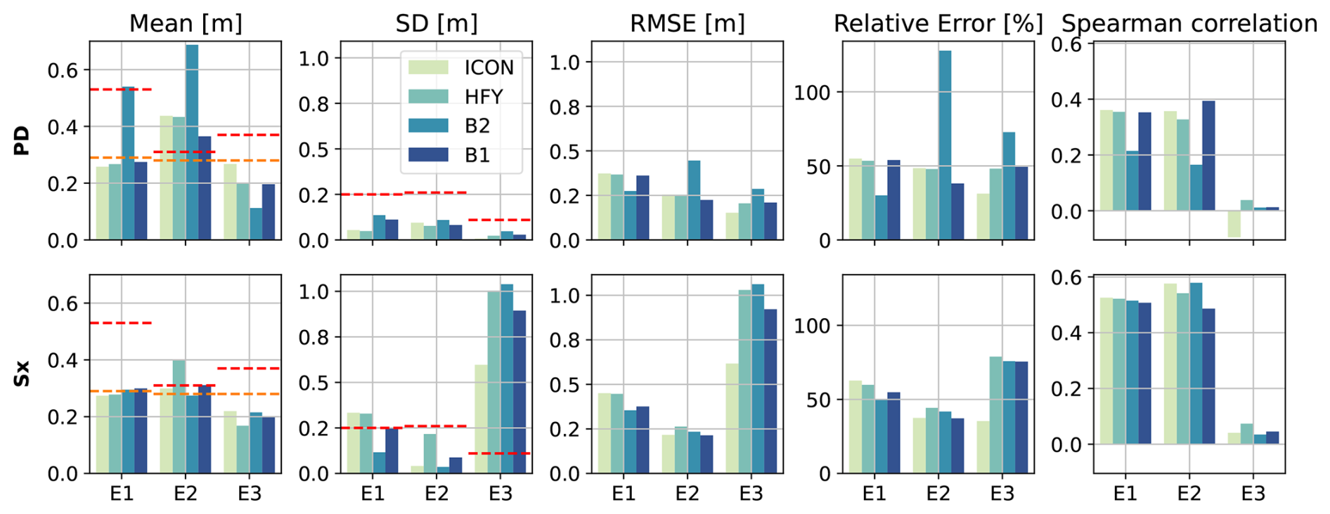
Figure 10 Metrics in comparison when using different wind input data for ΔHS PD and Sx modelling. The mean and standard deviation (SD) refer to ΔHS PD and Sx. The red and orange dashed lines correspond to the values derived from ΔHS TLS and HNW ICON ($\stackrel{\mathrm{‾}}{{\text{HNW}}_E}$ scaled by $\stackrel{\mathrm{‾}}{{\mathit{\rho }}_E}$). The error metrics RMSE, relative error and Spearman correlation refer to a comparison of ΔHS PD and Sx to ΔHS TLS.

5.1.2 Underlying DSM

With the growth of the snowpack during winter, the terrain surface changes. In addition, the snow-covered surface itself is dynamic and can evolve during an event, depending on the availability of erodible snow. In principle, predicting an event of new snow distribution based on terrain features, would benefit from using the most recent DSM, which is however in most cases not available. Using the DSM from 19 December 2023, we can compare the modelled results when using a snow-off DSM, or a more recent snow-covered DSM (Fig. 11). In our implementation we apply all models at the same spatial resolution of 0.5 m.

Overall, the results show only minor differences in model performance between the two DSMs. There is a slight decrease of RMSE and relative error (except for ΔHS Sx), and increase in Spearman correlation for ΔHS TPI, when using the more recent DSM, although the differences are very small. A likely explanation is that the terrain features dominating the model behaviour remain largely unchanged between the two DSMs, while the snow cover mainly smooths small-scale roughness and therefore results in a similar effective surface representation. In addition, this comparison is carried out relatively early in the winter season, which limits the geometric differences between the snow-off and snow-covered surfaces. However, we are aware that this result should be viewed with caution, as the extent of changes to the surface geometry depends strongly on the respective terrain features, the snow height and the snowpack conditions during each winter season.

In principle, the lidar data from an automated measurement station could provide updated information on the snow-covered surface and thus support the use of more recent DSMs in the modelling. However, the spatial coverage of the lidar measurements is currently limited and varies between time steps, particularly during snowfall. A consistent, spatially complete and temporally evolving DSM for the full study area is therefore not yet available within the current framework.

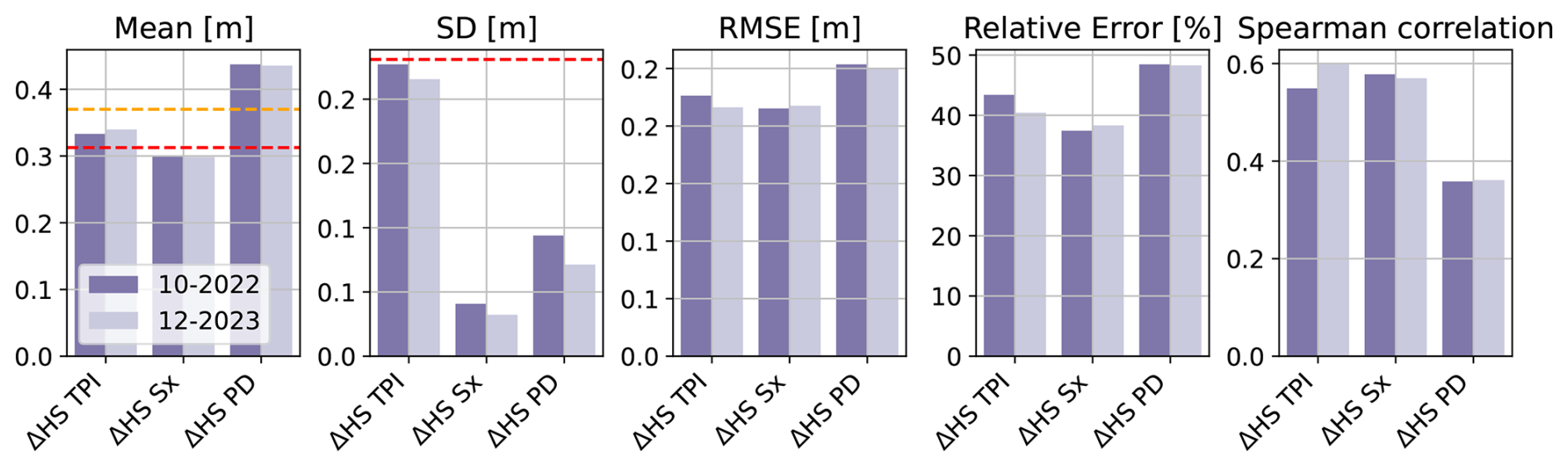
Figure 11 Metrics for ΔHS computed for E2, comparing the use of the snow-off DSM from 18 October 2022 (10-2022), or a more recent DSM with snow cover, in this case from 19 December 2023 (12-2023). The mean and standard deviation (SD) refer to ΔHS TPI, Sx and PD. The red and orange dashed lines correspond to the values derived from ΔHS TLS and HNW ICON ($\stackrel{\mathrm{‾}}{{\text{HNW}}_E}$ scaled by $\stackrel{\mathrm{‾}}{{\mathit{\rho }}_E}$). The error metrics RMSE, relative error and Spearman correlation refer to a comparison of ΔHS TPI, Sx, and PD to ΔHS TLS.

5.1.3 Precipitation and scaling input

The choice of precipitation or snow-depth input primarily affects the absolute scaling of the modelled ΔHS fields. In the main analysis, we use ICON-derived $\stackrel{\mathrm{‾}}{\text{HNW}}$ as mean precipitation input in order to assess the applicability of the models with spatially continuous meteorological data. We additionally tested a scaling based on the event-mean TLS-derived ΔHS. This eliminates (or reduces, in the case of the PD model, see Eq. 4) the mean bias, but the RMSE and relative error do not improve consistently, and the correlation scores remain similar (Fig. 12). This underlines that, in the current setup, the precipitation input mainly acts as an event-scale scaling factor, whereas the spatial patterns are largely determined by the respective terrain index or preferential deposition formulation. The partly increased RMSE values indicate that simply constraining the model to the observed event mean is not sufficient to improve spatial agreement. Instead, a key limitation is the scaling procedure used to transform relative terrain indicators into quantitative ΔHS. While many studies have shown that terrain parameters are related to spatial snow depth variability, a robust and transferable scaling from such indices to absolute ΔHS remains challenging, particularly across different and mixed event types, geographical regions and snow climates. The measured ΔHS are valuable for future model calibration and development. Their high spatial and temporal resolution can help to separate periods dominated by preferential deposition, redistribution, or mixed processes.

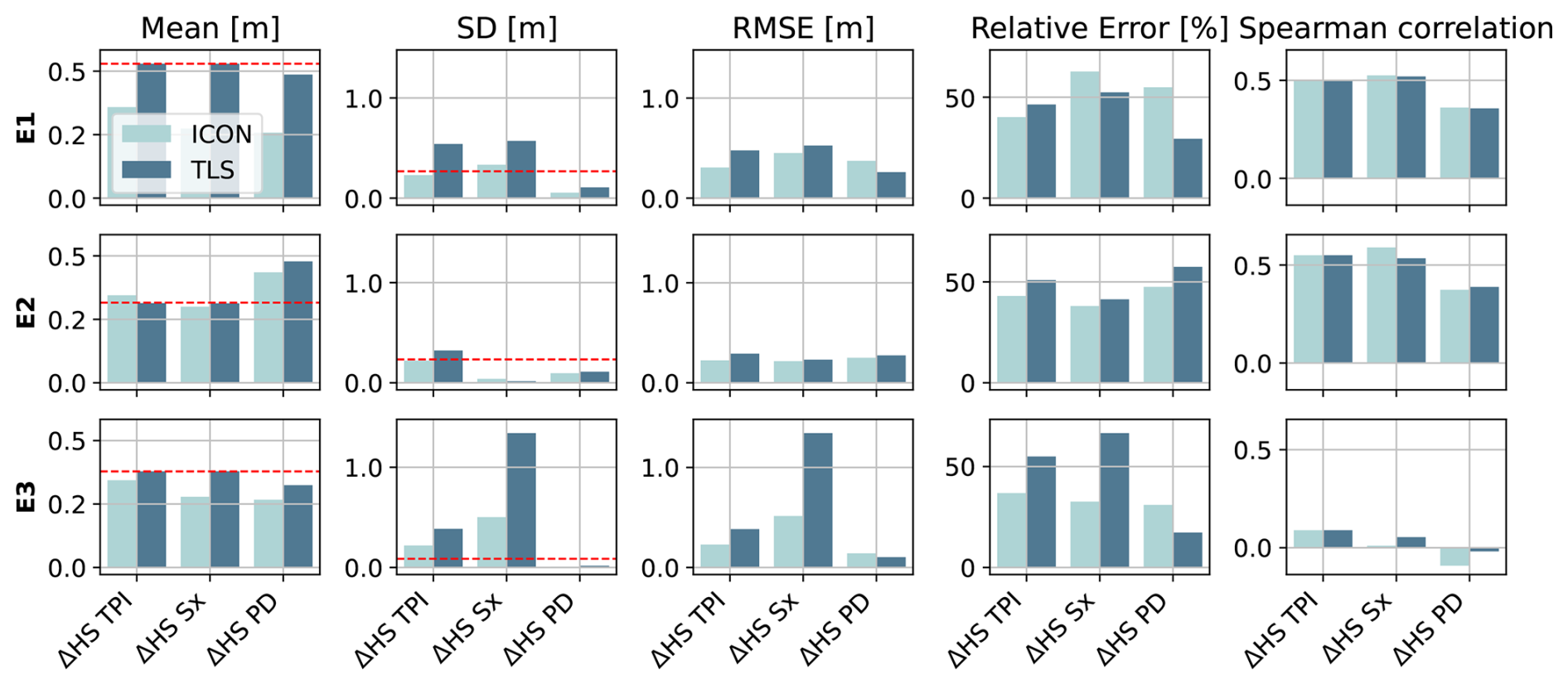
Figure 12 Metrics for ΔHS computed for all main events, comparing the use of ICON-derived $\stackrel{\mathrm{‾}}{\text{HNW}}$ (scaled by $\stackrel{\mathrm{‾}}{{\mathit{\rho }}_E}$) and TLS-derived ΔHS as scaling input. The mean and standard deviation (SD) refer to the modelled ΔHS for TPI, Sx, and PD. The red dashed lines correspond to the values derived from the measured ΔHS TLS. The error metrics RMSE, relative error, and Spearman correlation refer to a comparison of ΔHS TPI, Sx, and PD to ΔHS TLS.

5.2 Model applicability and limitations

In this study we tested the performance of various approaches to estimate the distribution of new snow or snow depth changes in an avalanche release area at very high temporal and spatial resolution. The results show that the tested low-complexity approaches can reproduce parts of the observed spatial snow depth patterns, but none of them fully captures the variability of ΔHS across all events. This reflects both the simplified process representation of the models and the fact that real snowfall events are always a mix of several processes. The following discussion therefore focuses on the applicability and limitations of each approach.

The simplest, most general approach is the use of topographic position index TPI. However, it depends only on one parameter, the radius of evaluation. It is thus not sensitive to any wind variations in snowfall events. This is visible in Fig. 6, where the snow depth distribution pattern is the same for all events. There is only slight variation in scaling, according to the input of precipitation. This can be viewed as strength, as it makes the model more generic which could be an advantage for mixed type events. However, it is also a limitation, because the distribution of ΔHS for preferential deposition or redistribution events strongly depends on the wind speed and wind direction and the approach using only the TPI can not be adapted to individual meteorological conditions.

The wind shelter index Sx mainly depends on the wind direction, which makes it adaptable to different events, although the wind speeds are not considered. On this rather small evaluation area, the rescaling of TPI and Sx to ΔHS strongly depends on the scaling method and the evaluated domain extent. This becomes evident for Sx in the example of E2, where there are only little areas that are wind exposed, so the scaling ratio becomes very small (α in Eq. 9 or 10), leading to very little variation of snow depths in the wind sheltered areas. In this study we use a scaling by mean and standard deviation, because when using the minimum and maximum (as suggested by e.g., Bavay and Egger, 2014) we saw almost no variations of ΔHS in our ROI, due to some large (or small) values in the evaluated extent of DSM. Another approach for improvement could be to link the scaling factor to wind speed. For example, the scaling factor leads to too much variation in ΔHS for E3, but it seems reasonable for E2, as wind speed and therefore ΔHS variability are greater there.

The presented model for ΔHS based on PD takes all lacking parameters into account that are mentioned above, by relying on statistical downscaling of coarse meteorological parameters (precipitation, wind speed and direction). This allows an adaption to individual snowfall events, and the downscaling is designed to be broadly applicable, i.e., it is very little dependent on the resolution or extent of the model domain. However, the PD model has been developed for a spatial resolution of 30 m, and is the first time applied at the high resolution of 0.5 m. As the model name suggests, the PD model is limited on the representation of the process of preferential deposition. In reality the distribution of new snow is always a combination of multiple processes, so especially with higher wind speeds when also snow redistribution occurs, or during warm periods impacting the snowpack, the model cannot describe the resulting snow distribution (see mixed and redistribution events in Fig. 7). For example, ΔHS PD overestimates the absolute ΔHSs in E2. Given the rather high wind speeds as well as the warm period at the beginning of this event, other processes than preferential deposition, have likely contributed to shape the snow distribution during E2. However, since the model downscales coarse precipitation and coarse wind, the overestimation of ΔHS could also be from inaccuracies in precipitation and wind input. The overall similar spatial bias pattern among the three models indicates that the distribution patterns agree, which suggests a possible improvement of the model performance by adjusting the absolute scaling to wind speed and precipitation. An explanation for the low spatial variability of ΔHS in E3, calculated with the PD model, is the change of wind directions during the period of the event. Opposite wind directions with similar wind speeds can even out the accumulated result.

All presented models strongly depend on the input of precipitation ($\stackrel{\mathrm{‾}}{\text{HNW}}$) and the scaling to ΔHS, using the density ρ of new snow. In this study we use ρs, derived from manual, daily measurements of HN and HNW at the measurement site WFJ. For comparison, we derived ρs for the same evaluation periods from the automated weather station at WFJ, which is placed a few meters next to the manual measurement location. The correlation values do not change, since ρ is only a linear scaling factor, but we found variations in the bias of up to 0.18 m across the models and events, in comparison to ρ derived from the manual measurements. An additional source of uncertainty is the ICON-derived $\stackrel{\mathrm{‾}}{\text{HNW}}$, which is taken from the hourly KENDA-CH1 analysis data. These data provide an observation-constrained and spatially consistent estimate of precipitation on a 1.0 km grid, but local snowfall amounts in steep alpine terrain can still vary substantially within a single grid cell. In our modelling framework, $\stackrel{\mathrm{‾}}{\text{HNW}}$ mainly acts as scaling input. Its uncertainty is therefore expected to affect primarily the absolute magnitude of modelled ΔHS. For this reason, we focus on the interpretation of the model results primarily on their ability to reproduce spatial snow distribution patterns.

The correlations between measured and modelled snow depth distributions in this study are broadly consistent with previous studies, although direct numerical comparison is limited because correlation metrics, spatial resolution, aggregation scale, and calibration strategies differ. For example, Schön et al. (2015) reported coefficients of determination (r²) of approximately r²=0.47–0.73 for measured snow depth changes and r²=0.32–0.53 for absolute snow depths, depending on search distance, terrain representation, and case study. Researchers obtained a higher agreement when measured snow-transport information was incorporated, such as Schön et al. (2018) reported correlation coefficients of R=0.78–0.86 for a modified terrain parameter combined with blowing-snow flux measurements. At coarser aggregation scales, Grünewald et al. (2013) found that locally calibrated statistical models explained 30 %–91 % of snow depth variability.

These limitations also indicate where future model development could build on the lidar dataset. A promising direction for improvement is the use of data-driven models that exploit the high temporal resolution of the lidar dataset. While machine-learning-based approaches for snow distribution have already been explored in previous studies, hourly lidar observations over several winter seasons provide a new opportunity to relate snow depth changes to meteorological and terrain parameters at event and sub-event scale. This makes it possible to test both simple regression-based approaches and more complex deep learning models for learning event-dependent snow distribution patterns from the observations themselves. Such approaches may help to better represent mixed situations, in which preferential deposition, redistribution, and additional snowpack processes act simultaneously. In addition, machine learning could also be used to improve specific components of the current workflow, for example by emulating local wind fields from terrain and coarse meteorological input, as in ongoing work based on the deep-learning model Devine (Le Toumelin et al., 2023). The dataset presented here therefore offers considerable potential not only for model validation, but also for the development of more flexible, data-driven snow depth models.

A promising application of the presented models could be the spatio-temporal completion of TLS measured snow depth maps. In Fig. 13 we show a first attempt, where we show the TLS-derived ΔHS, complemented with the ΔHSs modelled with TPI. Such applications may be particularly valuable when measurements are incomplete because of adverse weather conditions or terrain-related shadowing.

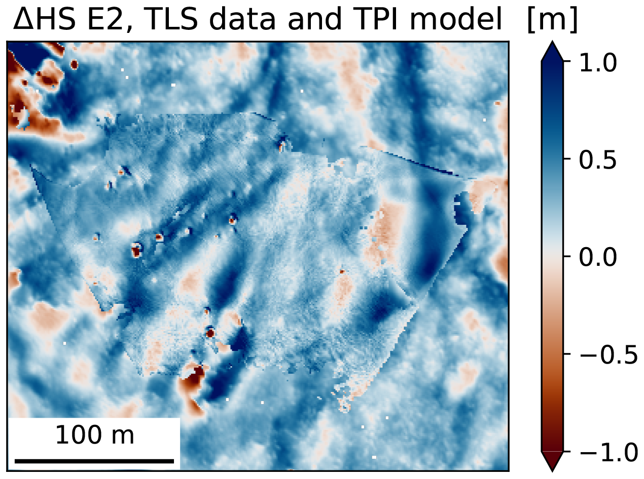
Figure 13 TLS data of E2 with gaps filled by the TPI model.

Our validation data is limited to a rather small area, due to the maximum measurement range of the TLS. Currently we use data from only one study site and evaluated three specific snowfall events. This has the consequence that we have only a certain variation of topography and meteorological conditions we can evaluate our models on. Furthermore, the measurements have local uncertainties in the range of 0.1–0.3 m (Ruttner et al., 2025a), which has to be considered in the interpretation of error metrics.

6 Conclusion and Outlook

The amount of new snow in an avalanche release area is crucial information for the prediction of avalanche danger, avalanche simulations, and applications like hazard indication mapping. Often, if at all, there are only snow depth measurements available from sparsely distributed flat field measurements, but no or little information within steep avalanche starting zones.

With our low-cost measurement setup we collect information on the snow depth distribution in an avalanche release area with high spatial and temporal resolution. Given weather- and line-of-sight-related gaps in the lidar data acquisitions, we evaluated different model approaches for describing spatial changes in snow depth to complement observations and support applied use. Specifically, we tested low-complexity, terrain-based modelling approaches based on low input requirements and low computational demand. We tested approaches using the topographic position index TPI, wind shelter index Sx and a model for preferential deposition PD.

Due to the differences in wind speeds and air temperature in each event, we assume different leading processes that form the measured distribution of ΔHS. We found the highest correlations of measured and modelled ΔHSs, by applying a basic rescaling of the indices TPI and Sx, for E1 and E2, being mixed events including snow redistribution by wind. E3, being a preferential deposition event with low wind speeds, has a rather homogeneous ΔHS distribution, therefore we did not find clear correlations, but the best performance in terms of RMSE was achieved by the PD model. Overall, the correlations are moderate (maximum Spearman of 0.58 for ΔHS Sx in E2), which indicates that we cannot fully explain the snow depth variability in avalanche release zones on such high spatio-temporal resolution using only TPI, Sx or statistical downscaling for snowfall. For mixed events, the best approach in our results is ΔHS derived from the TPI, although it does not take into account the wind.

The tested approaches which are considering the wind direction (Sx and PD model) would benefit from further optimisation and adaptation for high spatial resolutions of a few meters, since they were originally developed for larger scales and coarser spatial resolutions. We tested the PD and Sx model for the sensitivity to different input for wind data. Different wind data sources have a moderate impact on the model results, but with larger variations in the PD model results, which also takes wind speed into account. We could not derive a clear pattern of impact, for example regarding the proximity of the station to the test region. A better understanding of wind source impact on the model result will need further investigation. We also compared the results of ΔHS computations when using a snowfree- or more recent snow-covered DSM. The model performances are in most cases better on the snow-covered DSM, although the differences are small. Furthermore, we tested the effect of using TLS-derived event-mean ΔHS instead of ICON-derived $\stackrel{\mathrm{‾}}{\text{HNW}}$ as scaling input. This reduces the mean bias, but does not consistently improve RMSE, relative error or correlation scores. This indicates that a robust scaling from relative terrain indicators to quantitative ΔHS therefore remains an important point for future improvement.

In the future, the evaluations could be strengthened by testing additional study sites (to cover a larger variety of topography), and a larger variety of snowfall events. The testing of a combination of the different model approaches could probably better capture the events. For example, a preferential deposition model can be applied for a basin scale prediction and then further downscaled on the slope scale at very fine resolutions using the TPI or Sx indices. Although we started more frequent data acquisitions with a promising measurement approach, snow depth distribution measurements from avalanche release areas with high spatial and temporal resolution are still very scarce. By further extending measurement setups at more locations and collecting relevant meteorological events, we can increase our understanding of avalanche formation processes and evaluate new modelling approaches. With more complete and reliable databases of avalanche release areas, machine learning models could be developed to describe the complex loading of lee slopes during mixed-process snowstorm events.

Appendix A

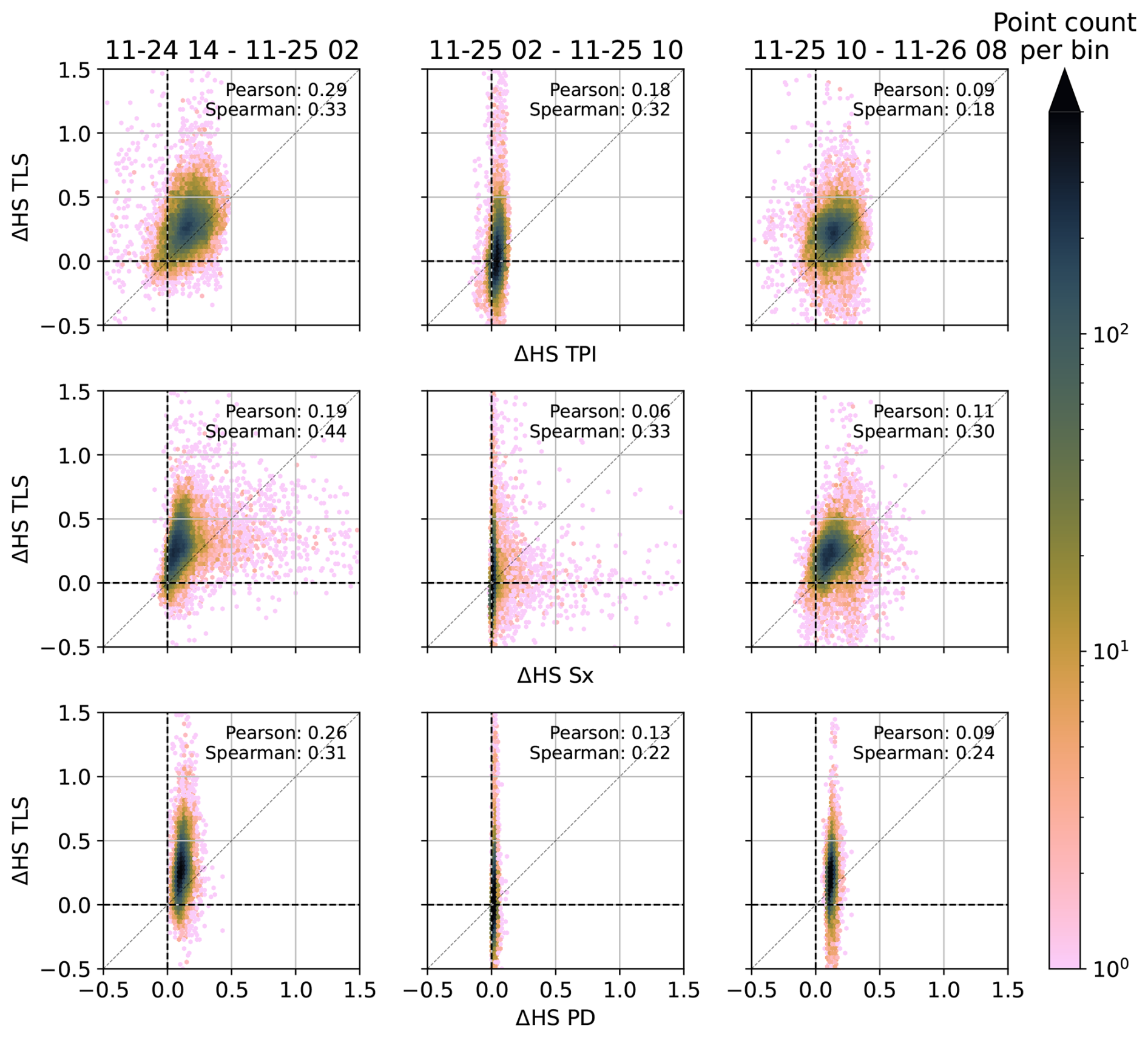
Figure A1 Scatter plots and Pearson and Spearman correlation coefficients of measured vs. modelled ΔHS for sub events for E1. Darker colours indicate a higher count per bin.

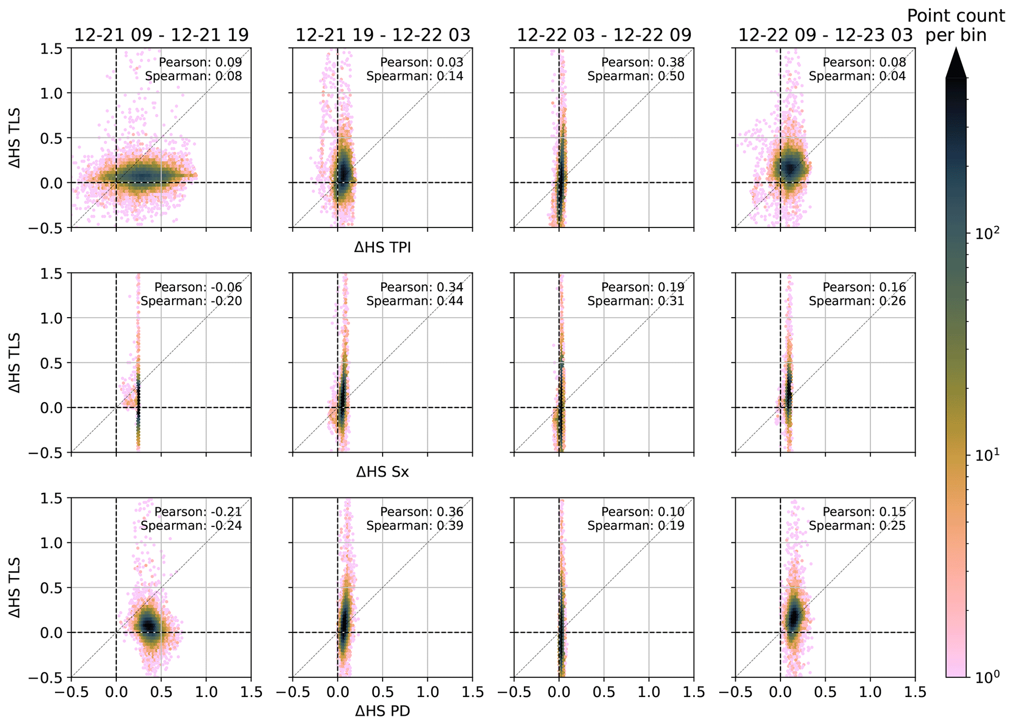
Figure A2 Scatter plots and Pearson and Spearman correlation coefficients of measured vs. modelled ΔHS for sub events for E2. Darker colours indicate a higher count per bin.

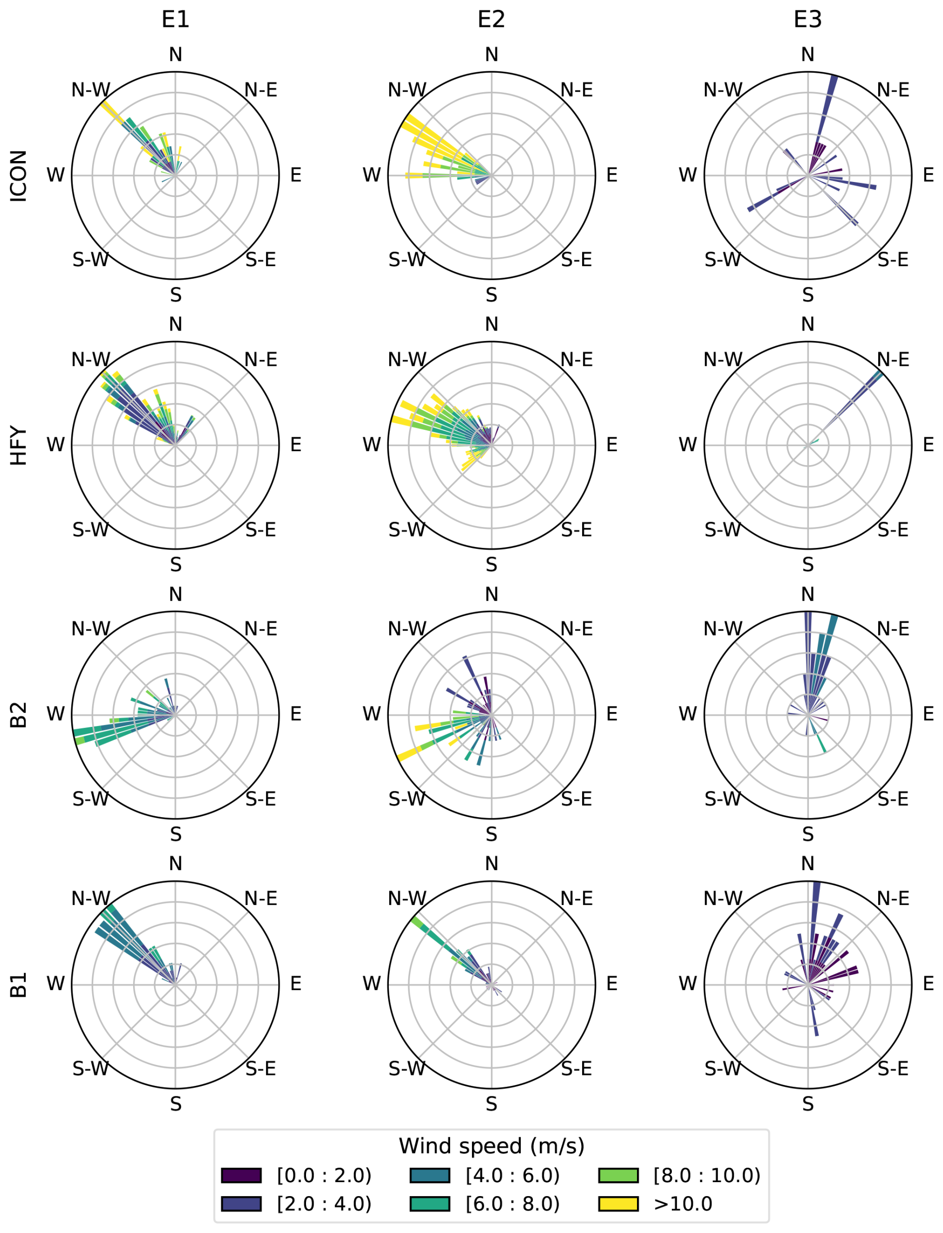
Figure A3 Overview of wind roses for events E1, E2, and E3, from the ICON model and measurement stations HFY, B2, and B1.

Table A1 Performance measures for different models and meteorological events (sub-events of E1). As bias we calculated the mean of the differences between the TLS measurements and the model, and the relative error refers to the median of relative errors. The best values per model are marked in bold numbers.

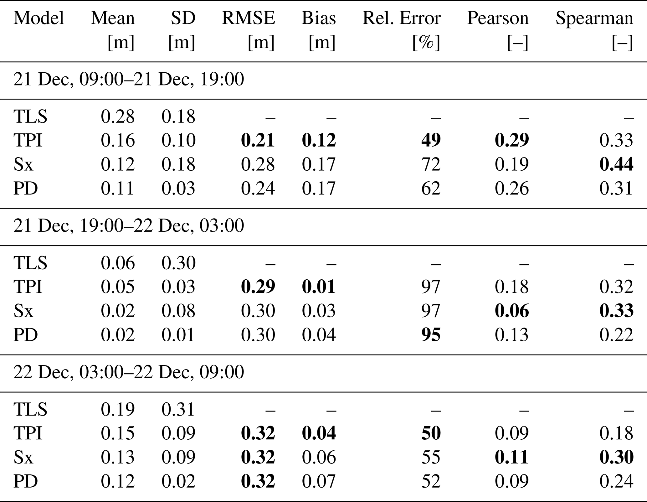
Table A2 Performance measures for different models and meteorological events (sub-events of E2). As bias we calculated the mean of the differences between the TLS measurements and the model, and the relative error refers to the median of relative errors. The best values per model are marked in bold numbers.