Freshly calved icebergs from Sermeq Kujalleq in Kangia, Greenland: is their blue ice temperate?

Blue ice on the freshly calved icebergs from Sermeq Kujalleq in Kangia, Greenland, is a striking feature which is not yet fully understood. Its extent and properties provide important insights into the flow dynamics of this polar ice stream, since it occupies the bottom-most quarter of the total ice thickness, and it has been conjectured that the blue ice is temperate.

Here, we document the phenomenon with ground-based time-lapse camera images, theodolite measurements, thermal imagery, and multi-spectral satellite imaging from Sentinel-2. The blue ice shows intriguing properties as its reflectance spectrum stands out from other types of ice. Clathrate hydrates or a high interstitial water content are possible hypotheses to explain such atypical reflectances. Within hours the blue ice whitens under the action of solar radiation, caused by opening of veins and cracks, and is potentially exacerbated by the dissolution of clathrates or the drainage of interstitial liquid water, which would indicate temperate conditions in the latter case.

Both hypotheses cannot conclusively explain the phenomenon. It remains to be demonstrated that clathrates persist long enough to move with the ice from the deepest part of the glacier trough to the calving front where overburden stress is considerably lower. Thermal imaging on the other hand refutes the hypothesis of high interstitial water content, indicating that blue ice is colder than white ice when using a standard thermal emissivity. Freshly calved icebergs offer a unique opportunity to explore properties and structures (layering, folding) of ice which was deformed at great depth within polar ice streams.

1 Introduction

The huge, freshly calved icebergs from Sermeq Kujalleq in Kangia (SKK, West Greenland; also known as Jakobshavn Isbræ) often feature portions with strikingly blue and green-greyish ice. This phenomenon, although not unique and also observable at several other polar ice streams, is iconic of SKK due to recurrent calving of blue icebergs with volumes of the order 10⁷–10⁸ m³.

Green and blue icebergs from beneath the Antarctic ice shelves have been documented (Warren et al., 2019) and likely originate from marine ice accretion. The situation at SKK does not allow for freeze-on ice formation. The ice stream is grounded and fast-moving such that the processes leading to blue ice formation take place at depth within the ice stream. Except from the qualitative conclusion that this blue ice could indicate temperate conditions (Lüthi et al., 2009), no quantitative investigations about the properties of such ice have been performed to date. If the blue ice is indeed temperate, such in-situ observations could be used to constrain numerical models of the polythermal structure of polar ice streams. Since the thickness of temperate ice has only been modeled or extrapolated from borehole measurements, such observations would form an important milestone in the understanding of the mechanisms of the fast flow of polar ice streams.

In this study, we investigate one of the most productive ice streams of the Greenland Ice Sheet (GrIS) in terms of calving flux (Rignot and Kanagaratnam, 2006; Mankoff et al., 2020) to catch a glimpse on englacial conditions to investigate properties otherwise observable only in deep boreholes and with considerable effort. As direct in-situ investigations of freshly calved icebergs would be logistically challenging and dangerous, our investigations rely on ground-based and satellite remote sensing. The characteristics of glacier ice were investigated with special focus on the possibility that the blue ice is temperate and contains liquid water.

2 Data and Methods

2.1 Study site description

The fast flow of SKK, one of the main ice streams draining 6.5 % of the GrIS (e.g. Rignot and Mouginot, 2012) has been thoroughly studied during the last decades. The ice flows through a bedrock through reaching a depth below sea level of 1500 m and an ice thickness of 2500 m (Morlighem et al., 2025). The surface velocity reaches 8 km a⁻¹ in the trough and up to 14 km a⁻¹ at the terminus (Joughin et al., 2011).

Deep boreholes were drilled through the ice stream to elucidate the mechanisms of fast flow (Iken et al., 1993; Lüthi et al., 2002). At the ice stream margins, temperate ice close to the bed was discovered at sites A, C and D (Fig. 1) but not at central site B where drilling stopped far above the bed. From modeled extrapolation of measured temperature profiles (Funk et al., 1994), it was concluded that a very thick layer of temperate ice resides within the trough. Together with convergent ice flow (Iken et al., 1993) the temperate ice contributes considerably to the observed fast flow. However, recent modeling studies demonstrated that the fast flow can also be explained by significant sliding (Shapero et al., 2016; Bondzio et al., 2017; Poinar et al., 2017).

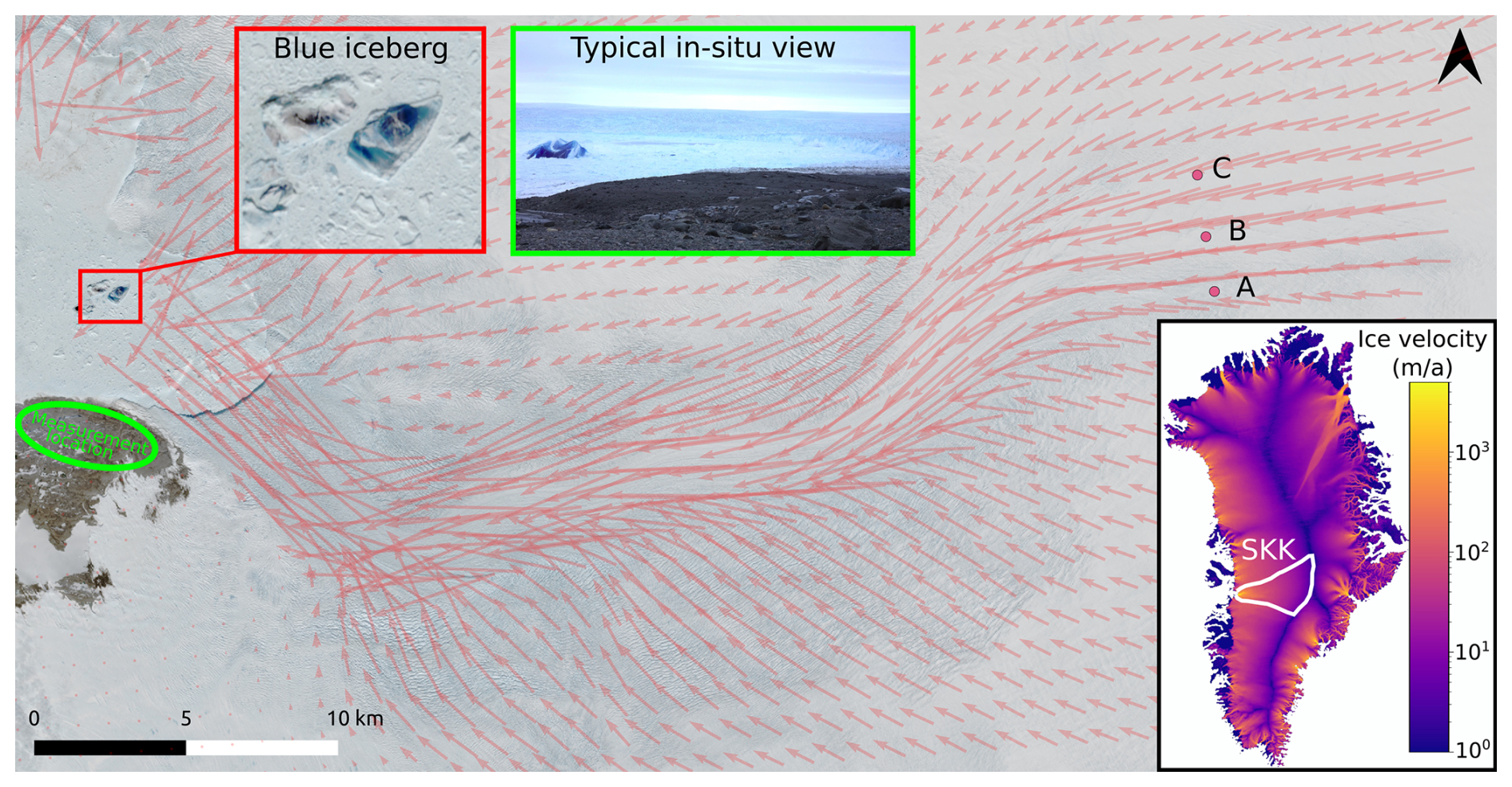
Figure 1 Illustration of the study site. Sentinel-2 satellite image of the SKK terminus area with calving front and freshly calved blue icebergs (red square). Velocity vectors (red) highlight the rapid and convergent flow in the ice stream (Joughin et al., 2011). Pink points with letters A, B, C indicate borehole locations. Inset shows the location of SKK on a map of GrIS surface velocities (Copernicus Climate Change Service, 2020). Satellite image: Sentinel-2 L2A, 14 May 2021, modified Copernicus Sentinel data.

2.2 Satellite multi-spectral imaging

Multi-spectral satellite imagery from the Sentinel-2 and Sentinel-3 platforms were retrieved from Sentinel Hub (2017–2023). We used Level-2A processing, an atmospherically corrected ortho-image representing the bottom of atmosphere (BOA) reflectance. Sentinel-2 provides 12 bands and has a revisit time of 1 to 2 d at SKK. It was used to derive reflectance spectra in the visible (VIS, 4 bands), near infrared (NIR, 6 bands) and shortwave infrared (SWIR, 2 bands) with a spatial resolution of between 10 and 60 m. Sentinel-3 passes every day and the true color images from the Ocean and Land Contour Instrument (OLCI) were used to determine the time of calving. However, its spatial resolution (300 m) was too coarse for the scope of this study.

Blue ice was identified on freshly calved icebergs using true-color Sentinel-2 images. To ensure the most uniform reflectance conditions, icebergs in shadow and those exhibiting specular reflection (very bright icebergs) were excluded. A catalog of 24 icebergs (or iceberg ensembles) featuring blue ice between 2017 and 2022 was created. For comparison, 24 white icebergs were chosen from many that could be found in the fjord. Finally, we also extracted mean reflectance from 4 shallow melt water ponds at the surface of icebergs, and the reflectance of a lake on land with no evidence of significant suspended sediments in the surroundings of the area (50.87° W, 69.09° N) on 17 August 2023.

From the 24 blue icebergs, 9 were tracked and the evolution of the reflectance spectra and blue color index was studied over 13 d. These 9 icebergs were divided into two groups: 6 of them calved between May and mid-August, when solar radiation was at its peak. Three others calved on the same day on 18 September 2021, when solar radiation had already significantly decreased.

The blue color in the visible spectrum was quantified with an index (referenced as blue color index) comparing the magnitude of the blue channel to that of red, green and blue channels (Sentinel-2 bands 4, 3, and 2).

$$\begin{array}{}\text{(1)}& \begin{array}{rl}{B}_{\mathrm{index}}& ={\displaystyle \frac{\mathrm{blue}}{\mathrm{red}+\mathrm{green}+\mathrm{blue}}}\\ & ={\displaystyle \frac{\mathrm{band}\mathrm{2}}{\mathrm{band}\mathrm{4}+\mathrm{band}\mathrm{3}+\mathrm{band}\mathrm{2}}}\end{array}\end{array}$$

To compare the reflectance spectra among each other, and with reference spectra, we quantify the magnitude differences between spectra using different measures: root mean square difference (RMSD), linear relationships using the Pearson correlation coefficient, and monotonic relationships using the Spearman's rank correlation.

2.3 Field measurements

Field measurements during 16 d were conducted on the south shore of SKK near the calving front (green ellipse on Fig. 1) between 3 and 18 July 2023. Numerous RGB pictures of freshly calved icebergs were taken from the camp and its vicinity, using digital cameras (Samsung NX300, Canon EOS 7D, Nikon D5200). Calving sequences were directly observed, and images from a stationary time-lapse sequence with 10 s interval were used (Canon EOS 70D).

The dimensions of freshly calved icebergs were measured by triangulation with a theodolite from two tripods. This method also allowed us to locate the various ice layers, especially blue ice and sediments, with an accuracy of 15 m in the horizontal and 3 m in the vertical (Lüthi et al., 2009). The theodolite (Leica TCR1101) was mounted consecutively on two survey tripods spaced 240 m apart in the vicinity of the camp. The distance to the target icebergs was between 2.5 and 6.0 km. Theodolite measurements were performed within 15 min after the ice mélange stopped moving after a calving event.

Thermal images were acquired to measure the thermal emissions of freshly calved icebergs with a pixel resolution of 5.5 m at 4 km distance. The thermal camera was a FLIR T440bx, with an uncooled infrared detector sensing between 7.5–13 µm, providing pictures of 320×240 pixels. Processing was performed with the open source software IRimage (Irujo, 2022). After alignment of thermal and RGB images, temperature and blue color index were extracted along a profile (presumably vertical before calving) on three icebergs with adjacent portions of blue and white ice.

3 Results

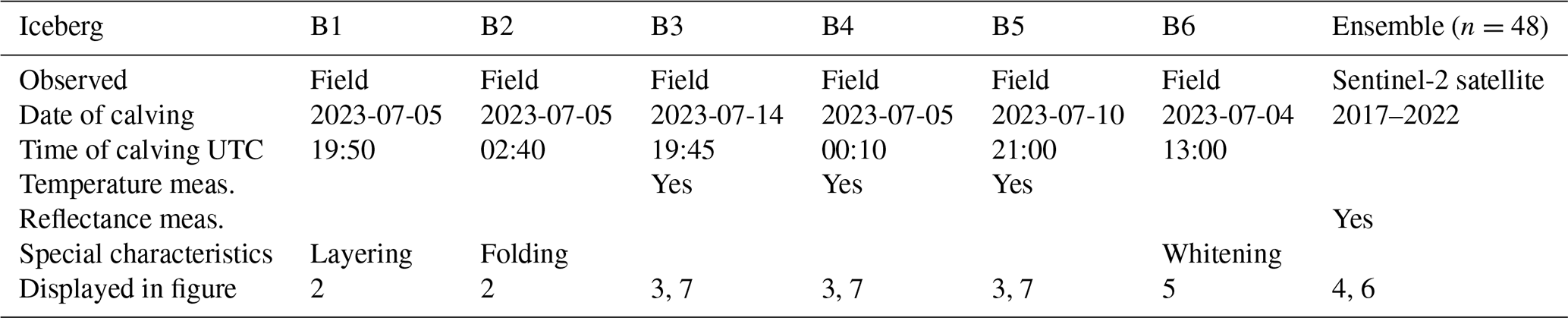
Six freshly calved icebergs with blue ice were analysed during the 2023 field campaign. From Sentinel-2 satellite imagery, a total of 48 icebergs with blue or white ice were identified. Table 1 summarizes the different icebergs observed in the field or with satellite multi-spectral imaging, the investigation methods used and references to illustrations.

Table 1 Summary of investigation methods and figures of the icebergs observed in the field or from Sentinel-2 satellite multi-spectral imaging.

3.1 Calving and appearance of blue ice

Based on numerous images taken over the past 20 years (Lüthi et al., 2009) and from observations in the field, blue ice is visible during most major calving events and appears to be independent of the position of the iceberg along the calving front, indicating that it exists across the entire width of the ice stream. There are two main ways to see blue ice appear during calving events. First, when an iceberg calves as a vertical slab and rotates backward, it horizontally exposes the formerly vertical cross-section of the ice stream, and blue ice is visible at its foot. Secondly, other icebergs calve but do not rotate immediately. First, they rise above the calving front due to buoyancy. Then, the part emerging from the water, which does not show blue ice, disintegrates. Next, still due to buoyancy, the deeper part of the iceberg rises to the surface and exposes the blue ice. The observations of these calving events allow us to affirm that blue ice was only observed in the bottom half of the glacier thickness.

3.2 Blue ice and bottom characteristics of the ice stream

The bottom structure of two icebergs is shown in Fig. 2. Iceberg B1 (Fig. 2, B1) exhibits a blue layer with a thickness of at least 200 m (the upper limit of blue ice cannot be deduced precisely due to white ice dust covering the iceberg). Immediately beneath the blue layer (left on the picture) lies a gray-greenish layer approximately 50 m thick, followed by a lighter layer of 120 m crossed by two thin layers of dark sediment or dust. The bottom consists of a 150 m thick layered structure, with sediment layers intertwined with blue or white ice. Iceberg B2 (Fig. 2, B2) shows an extended area of blue ice. A folded sequence including green-greyish ice, white ice and sediment layers is clearly observable, with an amplitude of around 100 m.

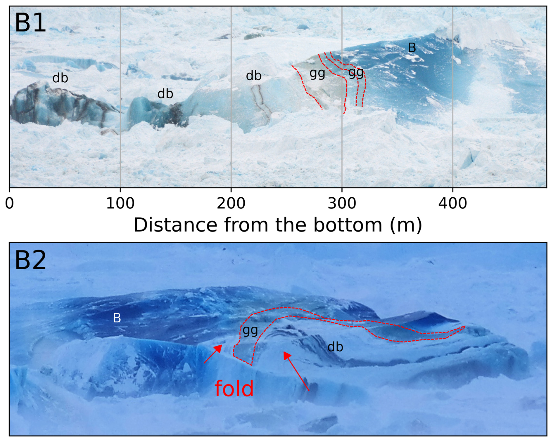
Figure 2 Icebergs B1 and B2 show large portions of blue (B) and green-greyish (gg, delimited in red) ice, and contain dark banded structures (db) and folds (red arrows). The scale in B2 could not be measured, but the displayed width amounts to ≈ 500 m.

3.3 Blue ice temperature from field thermal imaging

Surface temperatures from thermal imagery were determined along profiles on three icebergs (Fig. 3). Icebergs B3 and B4 are small and stem from the bottom half of the calving front thickness, whereas B5 is a full-depth tabular iceberg (description in Sect. 3.1). As seen by the thermal sensor, blue ice emits less infrared radiation than white ice. With emissivity set to 0.98 for both ice types, the inferred temperature of blue ice is colder than that of white ice. On iceberg B3, a clear temperature drop of 4 °C occurs between the white and the blue ice. This phenomenon is also visible on iceberg B4, with a temperature drop of 3 °C, but barely visible on iceberg B5, with a decrease of only 0.5 °C. Largest temperature variations are respectively 0.7, 0.3 and 0.1 K 10 m, all at the transition between white and blue ice.

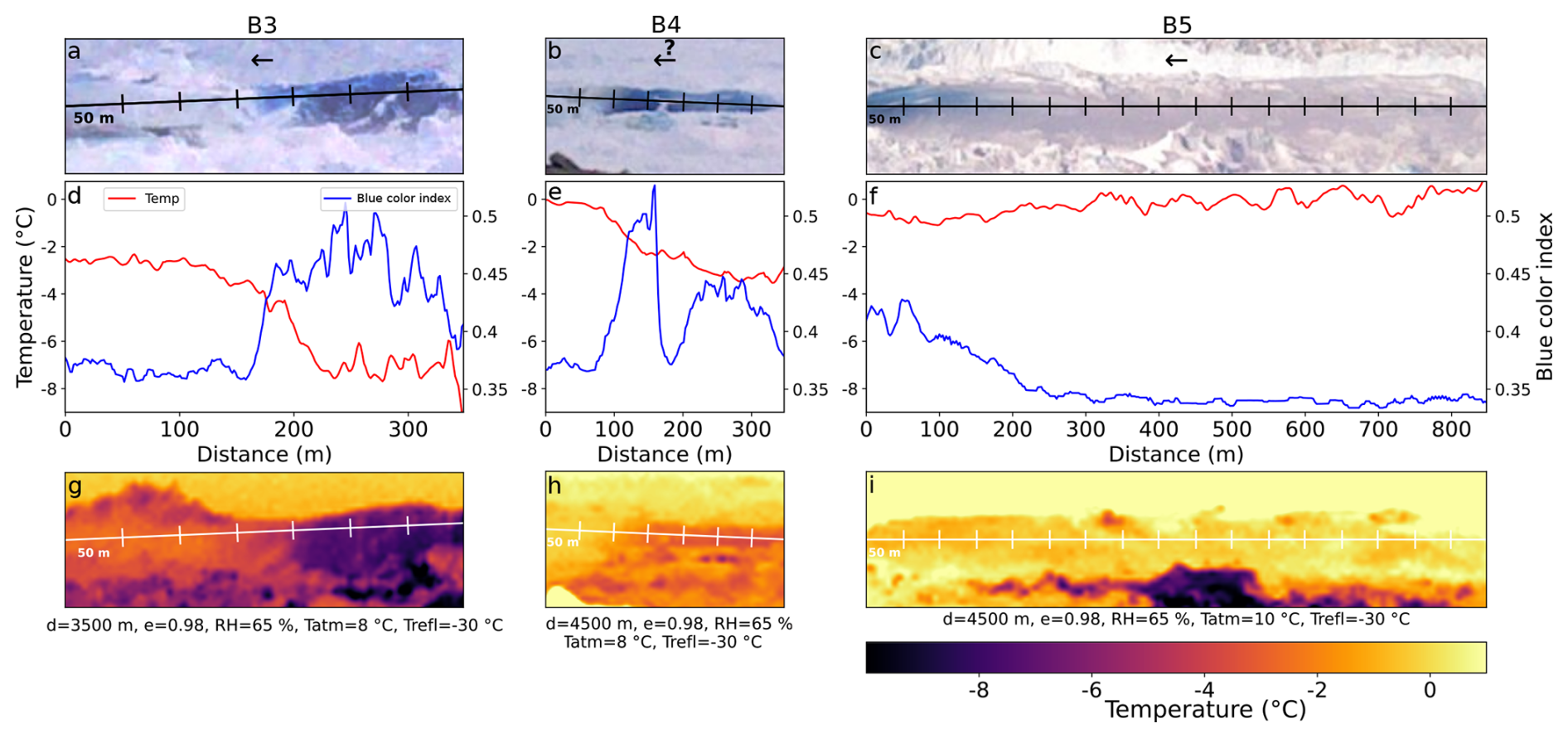
Figure 3 Temperature profiles along icebergs. The top row (a, b, c) shows photographs of icebergs. The arrows point downwards in the original iceberg orientation (orientation of B4 is uncertain). The middle row (d, e, f) shows inferred temperature from infrared emission (red curve, left axis) and blue color index (blue curve, right axis) variations along the iceberg. Distance starts from the lower extremity of the iceberg and goes towards its top. The bottom row (g, h, i) displays thermal images. Parameters used for processing are displayed below.

3.4 Blue ice characteristics from multi-spectral satellite imaging

3.4.1 Spectral properties and color after calving

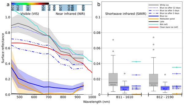
Mean reflectances were derived on the set of 24 blue icebergs and 24 white icebergs from Sentinel-2 multi-spectral satellite imagery. In the VIS and NIR, i.e. bands 1 to 9, blue icebergs have lower reflectances than white icebergs (Fig. 4a). Reflections on all bands are low except towards the blue/green bands. In the SWIR, on bands 11 and 12 (Fig. 4b), both blue and white icebergs show very low reflectances of the order 0.01. However, boxplot distributions show that blue iceberg reflectances are significantly smaller and distinct from that of white icebergs. Statistically, a Mann-Whitney U test returning p values of 10⁻⁴ for the bands 11 and 12 indicates that it is very unlikely that blue and white icebergs have the same reflectances in the SWIR.

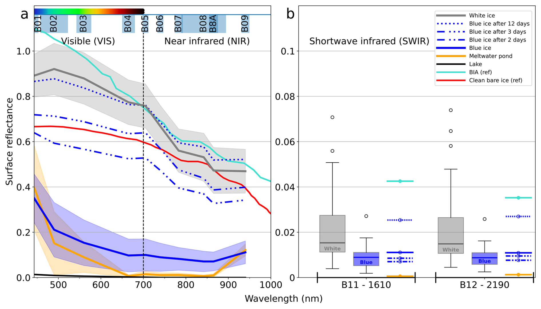
Figure 4 Sentinel-2 reflectances of different features in the VIS, NIR and SWIR domains. Mean blue ice reflectance (from 24 icebergs, in blue), white ice reflectance (from 24 icebergs, in grey) and supraglacial meltwater pond reflectance (from 4 icebergs, in orange) are displayed with standard deviation (colored area). The reflectance of a land-based lake is also displayed by a black line at the bottom, as well as references for blue ice in Antarctica (BIA) in turquoise and clean bare ice in red. The reflectance evolution of the set of 6 icebergs on days 2, 3 and 12 after calving is displayed with dash-dotted lines. In panel (a), bands 1 to 9 are drawn as a continuous spectrum. In panel (b), vertical axis is zoomed and SWIR bands 11 and 12 are displayed separately in boxplots.

These results are compared with the water reflectance from a lake on land and the meltwater ponds situated at the surface of four icebergs (an example of a pond is visible in Fig. 5). The reflectance of a lake shows low values throughout the spectra: 0.01 in the VIS, 0.001 in the NIR and SWIR. Except at band 1 and 9, freshwater ponds on icebergs show lower reflectances than the blue icebergs. The reflectance values and the spectra shapes in the VIS and NIR are very similar to those of the blue icebergs, confirmed by statistical analysis (Table 2). Significantly smaller values are only found in the SWIR, similar to those of the lake (0.001).

Table 2 Blue and white ice spectrum shapes (rows) are compared with different features (columns: freshwater ponds on icebergs, clean bare ice and BIA) to investigate the spectrum similarities. Values close to one indicate similar spectra. Best agreement between one feature among blue or white ice is shown in bold. Blue ice is also directly compared to white ice to show benchmark values before interpreting other statistics. See Sect. 2.2 for description of the statistics used.

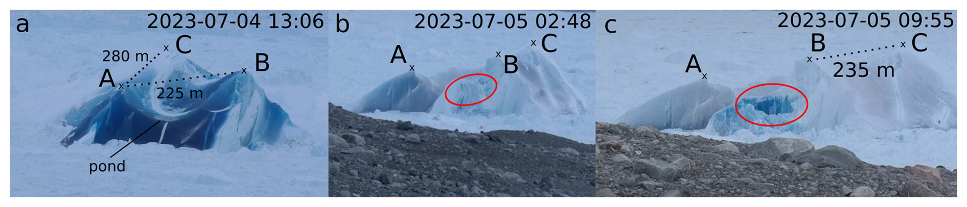
Figure 5 Evolution of the blue color of iceberg B6. Black crosses and dotted lines are used to show distances and orientation change of the iceberg. In panel (a), a pond is similar to those studied previously, except that here it is sea water trapped during calving, not melt water from the iceberg. In panel (b), an area about to collapse is circled in red. In panel (c), blue ice is revealed after the surface layer collapsed.

These results are qualitatively compared in Fig. 4 and statistically in Table 2 with literature references for clean algae-free bare ice (Stibal et al., 2017) and blue ice from Antarctica (BIA; Hui et al., 2014). White ice has similar values and shapes as reference clean bare ice in VIS and NIR, although values of the latter are slightly lower. It also shows very good agreement with the reflectance of BIA.

3.4.2 Evolution of iceberg color between 1 and 12 d

In what follows, we investigate the evolution of the reflectance spectra between 1 and 12 d of six icebergs that calved between May and mid-August (blue dash-dotted lines in Fig. 4). In VIS and NIR, reflectances strongly increase and reach values of the white ice. The gain is significant during the first 2 d with 60 % of the total change, after which they continue at a lower rate, reaching the range of white iceberg values 12 d after calving. In the SWIR, the reflectance first decreases around 30 % between day 0 and day 3, before increasing to values in the range of white icebergs on day 12.

Focussing on the visible range, the bleaching of the blue color can be observed qualitatively in Fig. 5. The ice turns to a blue-grey color, and then to white within 12 to 48 h. The process seems to happen only at the surface: 12–24 h after calving, a part of an iceberg that collapsed revealed blue ice underneath, which subsequently underwent the same bleaching process.

In a complementary fashion, we specifically quantified the blue color bleaching with satellite imagery in Fig. 6. We determined the day of calving and computed the blue color index (Eq. 1). The icebergs were divided into groups with stronger and weaker solar radiation, corresponding to satellite images acquired in late spring and summer (5 icebergs calved between May and mid-August) and autumn (mid-September). For both groups, the blue channel dominates immediately after calving, before decreasing and approaching the blue color index of white icebergs. An exponential decay curve can be fitted to both high and low solar radiation groups with respective time scales of 0.4 and 1.0 d. The bleaching of the blue color occurred faster under conditions with high solar radiation.

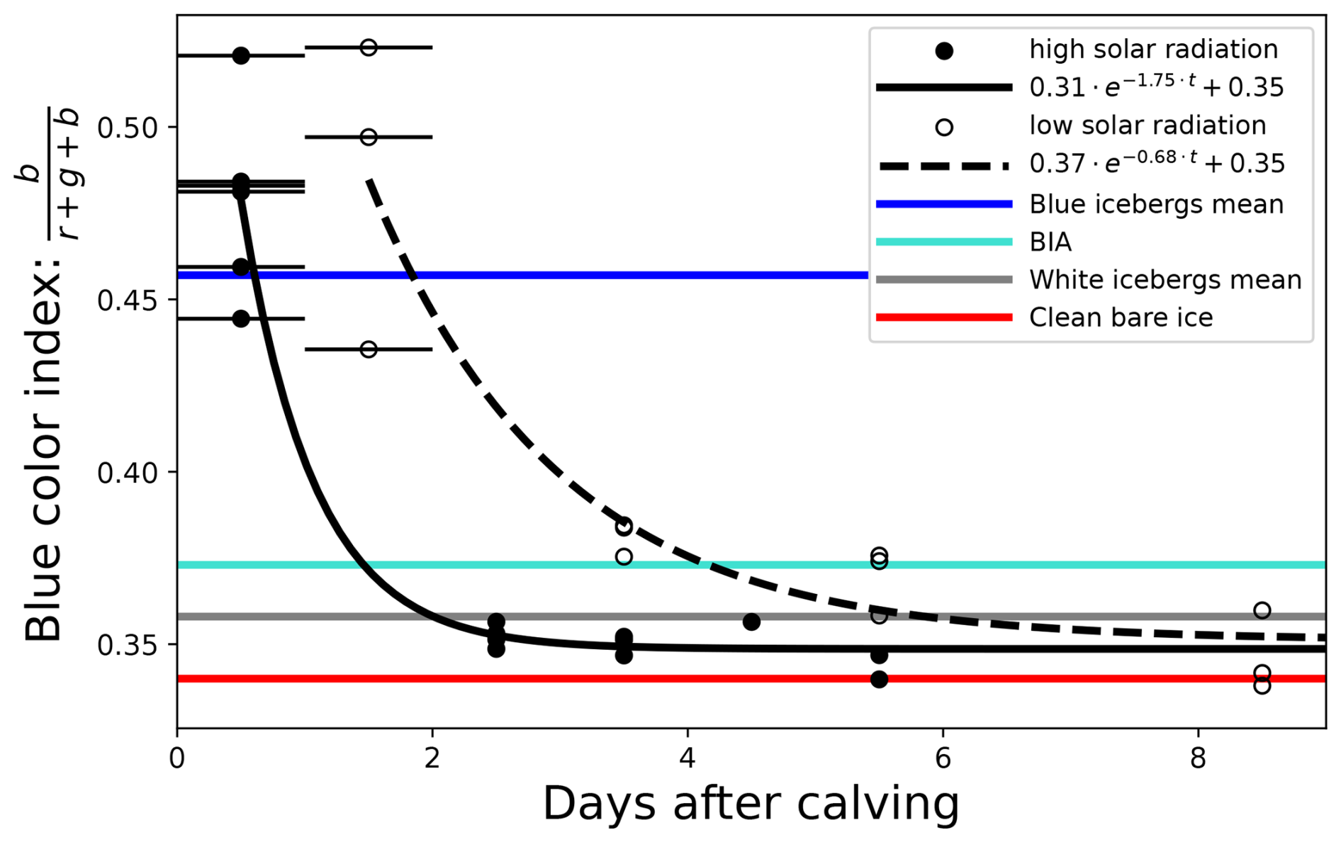
Figure 6 Evolution of the blue color index of initially blue icebergs in the cases of stronger and weaker solar radiation (solid and empty symbols), with exponential fits for each (solid and dashed lines). Comparison with index of white icebergs and references for BIA and clean bare ice are displayed as solid lines of various colors. Horizontal error bars indicate the uncertainty in the determination of the calving time (± 0.5 d) due to the almost simultaneous passage of the different satellites (only shown on the first symbols for readability).

4 Discussion

4.1 Blue ice reflectance

While the reflectance spectra of white icebergs exhibit the classical shape of glacier ice found in the literature (Stibal et al., 2017), blue icebergs show markedly distinct reflectances. They are more attenuated than the white ice, and also differ markedly from the BIA (Hui et al., 2014). In the NIR, blue icebergs show similar reflectances to those of a reflectance spectrum of water-saturated ice from Midtre Lovénbreen (Svalbard), which is certainly temperate (Pope and Rees, 2014). However, the saturated ice reflectance spectra shows a concave-downward shape, contrary to the concave-upward shape of blue icebergs from SKK. Shallow melt water ponds that form on icebergs and blue ice admittedly show similar reflectance values and concave upwards shape of the spectra, but the comparison does not lead further due to the distinct physical processes involved. On shallow melt water ponds, the light reflected on the submerged white ice surface passes through the water, which acts as a filter that blocks red light and transmits blue light, hence the blue color.

In what follows, we suggest reasons to explain why the spectral properties of blue ice differ from those of white ice. Several factors can influence the spectral properties of the ice and reduce its reflectance. Larger grain size or lower air bubble content can significantly reduce reflectance and could make the ice appear blue (e.g. Bohren, 1983; Dadic et al., 2013). Bi-directional reflectance also has an impact, especially on complex iceberg topographies (Winther, 1994). It however appears in these studies that the impact of larger grain size, lower porosity or lower viewing angle rather shifts the reflectance downwards, without altering the concave-downward shape of the spectra in the VIS and NIR. Contrary to the intuition that the BIA reflectance would resemble that of blue ice, the BIA reflectance obtained with an on-site spectroradiometer is surprisingly more similar to SKK white ice than to its blue ice. Because the color of BIA is attributed to large grain size and low air bubble content (both achieved through the overlying ice pressure over thousands of years, similarly to SKK white ice), this suggests that a different mechanism is behind the intriguing spectral properties of SKK blue ice.

4.1.1 High interstitial water content

Hypothesis 1 states that interstitial liquid water causes the reduced blue ice reflectance. Water, unless it contains large amounts of sediments, reflects little light at all wavelengths. This is demonstrated by the very attenuated reflectance of a land-based lake in the vicinity of the ice stream (Fig. 4), although here it is probably a directional reflectance under clear sky, and a better estimate would be a hemispheric albedo of 0.06 to 0.10 (Du et al., 2023). The presence of englacial liquid water in blue icebergs may explain their lower reflectance compared to white icebergs and therefore indicate that the blue ice is temperate. Liquid water in temperate ice would reflect less light than cold dry ice. Since temperate ice contains only 0.1 % to 4 % of liquid water (Pettersson et al., 2004), the reflectance would not be as strongly attenuated as that of water and could be in the range of our reflectance for blue ice. At this stage, this hypothesis lacks supporting evidence, such as direct comparisons with temperate ice reflectance of polar ice streams.

4.1.2 Refreezing and clathrates

There are two other possible explanations for the intensely blue color observed in the icebergs, but both are also not fully conclusive. Both hypotheses start with the observation that the blue color occurs because the ice does not contain any air bubbles. Hypothesis 2 assumes that recrystallization at high temperatures, and potentially melting and subsequent refreezing of the ice crystals, expel the small air bubbles and lead to less, but larger air pockets under very high pressure. Consequently, light penetrates deeper within the ice and absorption at red wavelengths make it appear blue. Hypothesis 3 builds on the fact that clathrate hydrates form under high pressure and at low temperature (Kuhs et al., 2000). During the formation of clathrates, gas molecules are encased within the crystal lattice of the ice molecules. As a result the air bubbles vanish from the ice and the reflectance is therefore low. According to Kuhs et al. (2000), nitrogen and oxygen, respectively, form clathrates at a pressure of 15 and 11.5 MPa at 273 K (and at a lower pressure for lower temperatures). This pressure is reached at an ice thickness of about 1650 m, which means that clathrates could form in the lower third of the ice column within the deep channel. This hypothesis is consistent with the depth at which blue ice was observed. After calving, blue ice rises to the surface where pressure is low, such that air bubbles can form the clathrates. This gradual formation of air bubbles would explain the gain in reflectance and the color change from blue to white on a time scale of hours to days.

For hypothesis 3 to apply, the rates of both clathrate formation and its inverse are crucial. The ice thickness at the calving front is 800–1000 m at the time of past and present blue ice observations (An et al., 2017). At an average flow speed on the lower 10 km of 20 m d⁻¹ the ice would be gradually depressurized from 15 to 9 MPa within 500 d. It remains to be demonstrated that clathrates remain stable under these conditions until the ice reaches the calving front. In addition, it remains to be explained how blue ice can persist for days in the interior of calved icebergs floating in the fjord, and therefore under low compressive stress. On several occasions floating icebergs were breaking apart (Fig. 5) and revealed intensely blue ice on the newly formed surfaces.

4.1.3 Impact of solar radiation on the reflectance evolution

The evolution of the spectra of blue icebergs seems directly linked to radiation, since icebergs calving at the time of the radiation maximum (May to mid-August) whiten faster than those calving in mid-September. Moreover, blue ice is still found under the whitening surface layer. We interpret this as the formation of a weathering crust at their surface. More radiation is absorbed along grain boundaries (Ambach, 1955), opening the veins between ice grains, which subsequently are filled with air and increase reflectance.

Assuming that the blue ice contains interstitial liquid water, it would drain from the ice by gravity when the veins open, thus explaining the strong reflectance increase and whitening of the blue icebergs. On the other hand, the formation of air bubbles from clathrates together with an opening of the veins could also explain the reflectance increase.

The quantification of the relation between the solar radiation and the blue color bleaching is only a crude approximate approach, because factors influencing the solar radiation (cloud cover, time of the day) are not taken into account here. The robustness of the method is also limited since the three icebergs from weaker radiation conditions calved on the same day. A larger iceberg ensemble is needed to assess the effect of weaker radiation. Further investigations should also involve determination of the time of calving using seismic data, and an approximate surface energy budget using temperature and solar radiation data. These data were not available over the Sentinel-2 image period.

4.2 Thermal imaging insights

4.2.1 Biases

Drawing conclusions from the FLIR thermal camera absolute temperature measurements is difficult. The algorithm converting the raw sensor values into temperature is very sensitive to the air temperature and can shift the measured object temperature by up to 1 K for a 1 K change in air temperature. Over distances of several kilometers, various surfaces (bare soil and ice) and changing altitudes, accurately estimating this parameter is impossible. However, relative temperature differences remain similar. On the other hand, the ice will warm up on contact with ambient air if the photo is taken a few hours after calving, reducing the temperature contrast (as is the case for B4), or if it was in contact with seawater before calving (a possible explanation for the almost uniform temperature profile of B5). Most importantly, there is no significant heat loss process; thus, the temperature of the ice observed can only be warmer than it was in the ice stream.

4.2.2 Comparison with borehole temperature profiles

We tentatively explore the similarity of the temperature profiles measured on initially vertical icebergs and the borehole temperature profile B measured in the center of the ice stream (Iken et al., 1993). We scale the vertical axis of the icebergs assuming a thickness of 900 m at the calving front and 2500 m within the ice stream. This linear scaling might not correspond to reality, as inference from different studies have shown (Funk et al., 1994; Lüthi et al., 2002, 2009). Ice color and temperature of the three icebergs from Fig. 3 are plotted against relative depth in Fig. 7.

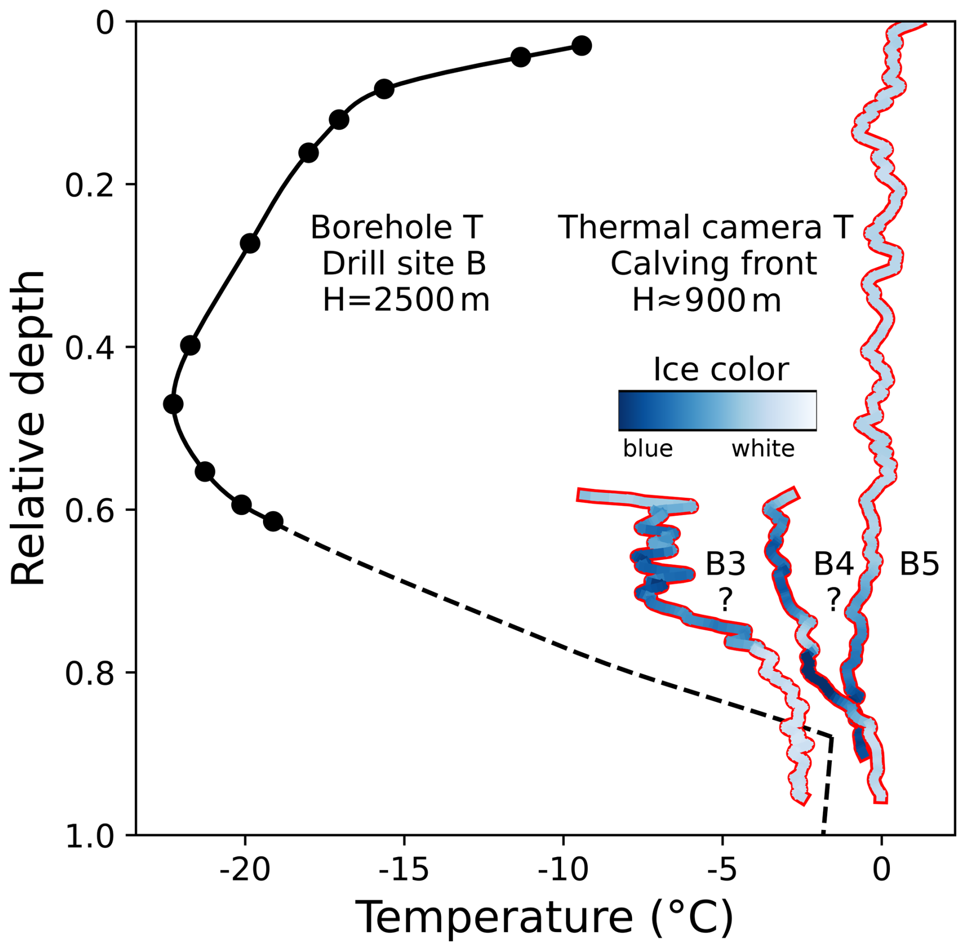
Figure 7 Temperature (T) and blue color index profiles scaled and located into the ice column. The icebergs B3, B4 and B5 from Fig. 3 are scaled and situated in the ice column to be compared with the temperature profile at drill site B (black line) and its extrapolation (dashed line) (Funk et al., 1994). Temperature is plotted on the horizontal axis as a function of relative depth. Ice color is represented by the color of the points (dark blue indicates blue ice). Vertical positions of B3 and B4 are uncertain.

Icebergs B3 and B4 are arbitrarily situated in the ice column displayed in Fig. 7. They feature a cold blue zone, with temperatures rising downwards to temperate conditions. The shapes of their temperature profiles are similar to that from the borehole, although the magnitudes are not the same. Since iceberg B5 calved as a nearly full-thickness iceberg where the top was preserved, we use the top as a reference to scale its depth. It shows nearly constant temperatures, except for the slightly colder blue ice at the bottom (0.7 to 0.9 relative depth), striking with the curvature from the borehole profile.

Given the employed linear vertical scaling, B3 and B4 graphically show that their blue ice might correspond to the core of very cold ice (−22 °C) measured in the borehole. In contrast, on B5, the cold core of blue ice is situated almost at the bottom of the ice stream, much deeper than the cold minimum at a relative depth of 0.5 in the borehole.

4.3 Contradictions about the blue ice temperature

Thermal emission temperature measurements contradict hypothesis 1 (high interstitial water content). Ice with a high interstitial water content must be at the pressure melting temperature, but cold blue ice cannot contain interstitial water. If the blue ice is indeed temperate, the thermal emissivity used in the processing the thermal infrared raw data has to be adjusted. The literature value of 0.98 was used to infer the temperature from raw sensor data, but it might be considerably lower than under laboratory conditions. For example, icebergs generally exposed flat surfaces and were seen with large viewing angles as a result of the small height-to-distance ratio. In the thermal infrared the directional ice emissivity drops to 0.82 with a viewing angle of 75° (Hori et al., 2006). Except for the viewing angle, various types of ice, such as sedimentary ice with variable air bubble content, grain size, clathrates or containing liquid water may influence the emissivity. However, no literature values on these characteristics in the thermal infrared could be found.

Emissivity ϵ is a crucial parameter in thermal imaging as it is used to account for the radiation from the surroundings reflected at the surface of the measured object (called reflectivity r) r=1−ϵ. The lower the emissivity, the higher the reflectivity. In our case, under clear sky conditions, decreasing the emissivity increases the computed object temperature. To investigate by how much this effect influences the derived temperature, the equation converting raw sensor values into temperature was inverted using a fixed emissivity.

We initially computed the ice temperature by processing the raw sensor values assuming an emissivity of 0.98. In the following, we assume that the blue ice is temperate (or at least, at the temperature of the adjacent white ice). Inverting the algorithm to compute the ice emissivity from the raw sensor values, the temperature was set to 0 °C. On iceberg B3, where the sensor values between the blue and white ice show the largest variation, the blue ice emissivity would drop to 0.70 if it were at the melting temperature (or to 0.80 for the temperature of the adjacent white ice). Given these calculations, it is possible that blue ice is temperate if it has a very low emissivity that makes it appear colder. Under these assumptions, the increase of ice temperature within a few hours (observed with fixed emissivity) can be translated into an increase of the emissivity (if the ice remains temperate), for example due to the drainage of the water from the temperate ice or the disappearance of clathrates.

4.4 Significance

In this study the properties of the blue ice observed on the freshly calved icebergs at SKK were investigated. These icebergs are particularly interesting because they offer a direct glimpse at the ice that is located deep within the ice stream and would otherwise only be accessible in boreholes. The blue ice layer is 200–250 m thick which amounts to one quarter of the total thickness of the ice stream.

The properties of the blue color and its time evolution after calving could not be unequivocally determined. From multi-spectral satellite imaging, attenuated reflectances are different from large-grained blue ice from Antarctica with low air bubble content and hint at a different cause. Clathrates or interstitial liquid water between ice grains are two possible explanations requiring further evidence. In thermal camera measurements the blue ice appears colder than white ice and suggests that it corresponds to the core of cold ice situated around mid-depth in the ice column, which contradicts the interstitial liquid water hypothesis. According to Lüthi et al. (2009), the vertical position of the blue ice is not necessarily at the bottom of the ice stream, as the icebergs show a complicated layering structure of sediment-rich ice, white, green and blue ice. If blue ice containing clathrates lies above white ice, why would the ice below not contain clathrates despite favorable pressure and temperature conditions? If the white ice below were temperate, interstitial water within temperate ice should rather promote clathrates with an enhanced air diffusion to nucleation sites (Ohno et al., 2010).

Conclusively answering the crucial question whether blue ice is temperate is not possible based on our measurements. If it were at the pressure melting temperature an implausibly low thermal emissivity of the blue ice would be required. On the other hand, such a thick layer of cold ice located near the bottom of the ice stream is difficult to explain regarding the high ice deformation rates, unless complex flow patterns from convergent ice flows have completely rearranged the original thermal structure.

In addition to the search for temperate ice, freshly calved icebergs reveal numerous structures (layers of different colors, large-scale folds) that are directly linked to complex and variable flow dynamics. The tributaries merging into the main ice stream likely create these complex structures, certainly accentuated by flow variability. These observations may confirm the numerical modeling of the fold formation in a convergent flow with a bottom layer of temperate ice (Zhang et al., 2024). Understanding these observations hinting to complex flow patterns requires comparison of detailed numerical modeling results with complementary sets of field observations to better constrain the mechanisms of fast ice stream flow.

4.5 Pathways for further research

The limitations of our methods are due to the relatively coarse spectral resolution of Sentinel-2 (10 to 60 m depending on the bands), inaccurate processing parameters (air temperature, emissivity) and altered ice temperature (heat from the sea, air) in thermal imaging. To resolve the contradictions discovered in this study, and to better understand the fast flow mechanisms of SKK in relation to the blue ice layer, drilling a borehole down to the bedrock in the center of the ice stream is certainly the most desirable method. However, to remain consistent with the relatively simple methods used in this study, we recommend the following research. (1) Drill into freshly calved icebergs, measure temperature and take ice samples. Such work would be possible from helicopters, if readily available, and might soon be achievable with sophisticated UAVs (drones). (2) Use hyperspectral satellites such as EnMAP or PRISMA to derive reflectance spectra with high spectral resolution and focus on liquid water absorption bands to infer temperate ice. Alternatively, fly a multi-spectral or hyperspectral UAV to obtain better spatial resolution. The latter method would also allow to study the properties of the thinner green-grayish layers possibly resulting from a high dust content originating from the late Wisconsin period (Lüthi et al., 2002). Linking the properties and their evolution of blue and green ice would provide a better understanding of the underlying processes. (3) Track the streamlines from where blue ice appears on the fjord surface. If only central streamlines, where fjord depth exceeded 1600 m for long distances, show blue ice, but not adjacent streamlines, this would be a strong argument for the clathrates (hypothesis 3).

5 Conclusions

By providing a direct view of the ice deeply buried in the ice stream, the numerous freshly calved icebergs from SKK have a large potential to better understand the complex and fast flow dynamics of this ice stream. In this study, we used satellite multi-spectral and thermal imaging to better constrain the characteristics of the 200–250 m thick layer of blue ice, which is not always situated at the bottom of the ice stream. We are not able to ascertain that blue ice is temperate since there are possible hints of liquid water content using satellite multi-spectral imaging, but thermal imaging shows that the ice is not at the melting temperature. Clathrates appear to be a plausible explanation, although pressure conditions might not be fulfilled in the terminus section of the ice stream. Further research should determine the origin of the atypically low reflectance, such as interstitial water content or clathrates, and also provide better constraints on the emissivity – temperature relation. Finally, results from the present study invite future SKK modeling studies to go beyond the purely viscous flow of the ice. Folding, faulting and stick-slip motion are consequences of complex merging processes in the convergent flow that should be modeled for accurate future predictions.