Investigating the drivers of wintertime Southern Ocean sea-ice leads using random forest algorithms

Sea-ice leads and coastal polynyas play a crucial role in regulating ocean-atmosphere energy exchange, yet the physical drivers controlling their variability across the Southern Ocean remain unquantified. This study uses a machine learning approach based on random forest regression with permutation importance analysis to identify the main drivers of Southern Ocean leads and coastal polynyas during winters (April–September, 2003–2023). The model integrates nine predictors representing atmospheric (wind speed, zonal u and meridional v wind components, wind divergence, sea-level pressure), oceanic (surface current speed), and sea-ice kinematic variables (ice velocity, ice divergence), together with a seasonal descriptor (month). Evaluated on independent test data, the model achieves a correlation of r= 0.70 at the pan-Antarctic scale and r= 0.63–0.82 across regional sectors. Relative importance analysis indicates that the zonal u wind (17.7 %), current speed (13.9 %), wind speed (12.9 %), meridional v wind (12.2 %), and ice divergence (11.2 %) together account for ∼ 68 % of the model’s total permutation importance. Regional analysis reveals sector-specific drivers: the Weddell Sea is primarily controlled by zonal u wind and ocean currents; the Indian and Pacific Ocean sectors by directional wind forcing; and the Bellingshausen–Amundsen Seas are influenced by ocean currents and meridional v wind. An analysis focused on coastal areas shows that current speed dominates in the nearest coastal zones (0–50 km) at the pan-Antarctic scale, and including a polynya dataset improves r values from 0.73 to 0.89 in these zones. However, the model does not fully resolve fine-scale structures evident in observations, hence a notable portion of the lead frequency variance still remains unexplained, which points out that the individual contribution of drivers for lead formation largely depends on local conditions and coastal geometries.

1 Introduction

Sea-ice leads, i.e. narrow linear cracks or elongated openings within the consolidated ice pack, play an important role in the climate system by mediating the exchange of heat, moisture, and gas between the ocean and atmosphere (Alam and Curry, 1997; Marcq and Weiss, 2012). When these openings expose relatively warm ocean water to the cold atmosphere, they trigger strong upward fluxes of sensible and latent heat, modify surface albedo, and influence boundary-layer stability (Lüpkes et al., 2008; Heinemann et al., 2022; Tian et al., 2025). As leads refreeze, they promote new ice formation and brine rejection, which in turn alter local salinity, increase water density, and contribute to deep-water formation and regional ocean circulation (Smith et al., 1990; Key et al., 1993; Ohshima et al., 2013). Beyond their thermodynamic significance, leads act as ecological and biogeochemical hotspots, providing habitats for marine fauna and serving as potential sources of methane emissions (Stirling, 1997; Kort et al., 2012; Damm et al., 2010). Through the ice–albedo feedback mechanism, an increased lead fraction enhances solar radiation absorption, which accelerates sea-ice thinning and amplifies regional climate feedbacks (Curry et al., 1995; Nihashi and Cavalieri, 2006). Consequently, lead variability strongly influences air–sea coupling and ocean circulation in both hemispheres (Vihma et al., 2014; von Albedyll et al., 2022).

The Southern Ocean represents a complex environment for studying lead dynamics due to the interplay of strong atmospheric forcing, intricate ocean circulation, and variable bathymetry (Holland and Kwok, 2012). Lead formation and variability are driven by both atmospheric processes, such as wind stress, and sea-ice dynamic processes, such as ice divergence, as well as oceanic circulation patterns (Reiser et al., 2019; Wang et al., 2023). Recent studies using thermal-infrared remote sensing have enabled the detection of sea-ice leads through surface temperature anomalies derived from the Moderate Resolution Imaging Spectroradiometer (MODIS), providing daily lead maps at a 1 km² spatial resolution (Reiser et al., 2020). However, frequent Antarctic cloud cover limits continuous observation and introduces substantial gaps in daily lead data.

To address these limitations, Dubey et al. (2025a) developed a gap-filled monthly climatology of lead frequency (LF) for winter months (April–September) between 2003 and 2023, offering a consistent long-term dataset for the Southern Ocean. Their analysis revealed ubiquitous and spatially heterogeneous lead occurrence, with pronounced maxima along coastal regions, continental shelf breaks, and key bathymetric features such as Maud Rise (∼ 66° S, 3° E) and Gunnerus Ridge (∼ 67° S, 34° E). Increased LF values (> 0.25) were observed particularly along the Weddell and Ross Seas shelf breaks, where leads frequently align with underlying topographic gradients (Reiser et al., 2019; Dubey et al., 2025a). Along the Antarctic coastal margins, open-water features also include coastal polynyas that form along ice shelves and landfast ice edges. These coastal polynyas share many physical drivers with pack-ice leads and play a similarly important role in mediating air–sea energy exchange, new ice formation, and dense shelf water production (Morales Maqueda et al., 2004; Golledge et al., 2025). To provide a more complete representation of wintertime leads with small-scale polynya activity across the Southern Ocean, the monthly coastal polynya dataset of Lin et al. (2024) is incorporated into the LF target variable in this study, enabling a combined analysis of both pack-ice leads and coastal polynyas within the same RF regression framework.

While several studies have described lead distributions and temporal variability in both polar regions (Wang et al., 2016; Reiser et al., 2019; Willmes et al., 2023; Dubey et al., 2025a), a comprehensive quantitative framework for identifying and ranking the physical drivers, and quantifying the relative importance of atmospheric, oceanic, and ice-dynamic controls on Southern Ocean leads and coastal polynyas is still lacking. This knowledge gap limits the representation of lead/coastal polynya related processes in coupled climate models and limits our capacity to assess how future changes in atmospheric or oceanic forcing might influence lead dynamics and their feedback on the polar climate system (Zhang, 2014; Rheinlænder et al., 2022).

The non-linear nature and multi-scale interactions among these drivers are difficult to capture using traditional linear statistical approaches. Machine-learning methods, particularly random forest (RF) regression models (Breiman, 2001; Biau, 2012), offer a strong framework to capture such non-linear relationships among multiple predictors without requiring predefined functional assumptions. In polar research, RF models have shown strong performance in diverse applications such as sea-ice drift calibration (Palerme and Müller, 2021; Zhang et al., 2024), forecast of sea-ice concentration (Chi and Kim, 2017), and ice-type classification (Shen et al., 2017). Beyond prediction, they also provide interpretable measures of variable relative importance through permutation-importance-based methods (Strobl et al., 2007), enabling identification of dominant drivers on lead formation.

Earlier work primarily focused on describing the spatial distribution, seasonal cycle, and long-term trends of LF derived from satellite observations (Dubey et al., 2025a; Reiser et al., 2020). However, an explanatory framework that integrates multiple predictors to model LF and identify the relative importance of individual drivers has not yet been developed. This study addresses this gap by developing an RF regression model to reconstruct LF across the Southern Ocean using predictors from the atmosphere, sea-ice and ocean for the period from 2003 to 2023 (April–September).

Using the gap-filled monthly LF dataset of Dubey et al. (2025a) combined with the coastal polynya dataset of Lin et al. (2024), this study has three main objectives. First, to quantify the contribution of key predictor variables to LF variability across the Southern Ocean. Second, to identify and rank the dominant drivers, and evaluate their relative importance for the pan-Antarctic region and five sub-sectors (Weddell Sea, Indian Ocean, Pacific Ocean, Ross Sea, and Bellingshausen–Amundsen Seas). Third, to assess the key coastal processes, including regional variations in model performance and predictor importance.

This study is structured as follows. Section 2 introduces the lead and coastal polynya dataset used as the target variable, outlines the atmospheric, ice-dynamic, and oceanic predictor variables, and describes the RF regression methodology. Section 3 presents the model performance using the test dataset for the Southern Ocean and its five regional sectors including coastal regions, evaluates predictor importance and the contribution of incremental predictors, and highlights the monthly model performance for each winter month. We discuss the results in Sect. 4, and finally, Sect. 5 concludes our work.

2 Data and Methods

2.1 Sea-ice lead frequency as target variable

This study uses the monthly LF dataset by Dubey et al. (2025b) for the Southern Ocean covering the months from April to September, 2003–2023. The dataset serves as the target variable in the RF regression framework. Monthly LF data are based on thermal infrared satellite imagery, which was used to detect leads as surface temperature anomalies in cold winter sea ice (Reiser et al., 2020). Monthly LF values were computed from daily lead observations as the fraction of clear-sky days during which a grid cell was identified as a lead (Dubey et al., 2025a). The LF represents a temporally integrated quantity indicating the number of days a pixel is covered by a lead during a specified period relative to the number of available clear-sky observations.

To provide a more complete representation of wintertime open-water activity along the Antarctic coastal margins, the coastal polynya dataset of Lin et al. (2024), was incorporated into the LF target variable. This dataset provides daily records of coastal polynya areas around Antarctica derived from passive microwave satellite observations, and is used here to supplement the MODIS-derived LF, which does not capture larger open water or thin ice areas (polynya-scale) explicitly. A monthly polynya frequency is therefore calculated based on the daily binary data. The year 2012 is excluded from the analysis because the polynya dataset is not available for that year. The combined dataset includes both pack-ice leads and coastal polynyas (LF), enabling a more physically complete analysis of wintertime lead variability across the Southern Ocean. We provide results, however, also for the leads-only data set (LF without polynyas, LFWP) to highlight the specific benefits that the polynya dataset can contribute.

For use in the RF framework, the 1 km² monthly LF data were spatially aggregated to a 2° latitude × 5° longitude grid (for basin-scale analysis) and 10×10 km² (for coastal analysis), respectively. This aggregation is meant to balance spatial resolution with computational efficiency while aligning with the resolution of predictor variables.

2.2 Predictor variables

To investigate the drivers of lead and coastal polynya formation, this study compiled nine input predictor variables for the same period as the target variable, grouped into four categories: atmospheric forcing, sea-ice kinematics, oceanic currents, and temporal descriptor.

Atmospheric predictors include the zonal u wind and meridional v wind components of the 10 m wind, 10 m wind speed, horizontal wind divergence, and sea-level pressure from the ERA5 reanalysis (Hersbach et al., 2020) produced by the European Centre for Medium-Range Weather Forecasts (ECMWF) and obtained from the Climate Data Store (CDS) of Copernicus Climate Change Service (C3S). ERA5 provides hourly atmospheric fields at approximately 31 km resolution, which were temporally averaged to monthly means and bilinearly interpolated to the analysis grid. The zonal u wind and meridional v wind components explicitly resolve the directional structure of near-surface wind forcing, capturing both the large-scale atmospheric circulation patterns and the local wind-driven divergence that mechanically fractures the ice cover and initiates lead opening (Kimura and Wakatsuchi, 2000). Wind speed and divergence represent the principal mechanical forcing for ice motion and lead opening, capturing both direct effects through wind shear and indirect influences via pressure gradients. Wind divergence is directly used from the ERA5 reanalysis for the 10 m wind field. Sea-level pressure accounts for large-scale synoptic variability that modulates wind stress and convergence–divergence patterns over the ice pack (Tschudi et al., 2019; Hersbach et al., 2020).

Sea-ice kinematic predictors in this study consist of ice velocity, and ice divergence. Ice velocity and divergence are derived from the Polar Pathfinder Daily Sea Ice Motion product (Tschudi et al., 2019) provided by the National Snow and Ice Data Center (NSIDC). This product integrates motion estimates from passive microwave sensors, visible and infrared satellite imagery, together with atmospheric reanalysis winds to generate daily ice drift vectors at 25 km spatial resolution. Ice divergence was calculated from the ice velocity components using centered finite differences. Grid cells containing land or coastline were masked using the land-sea mask of the analysis grid prior to the divergence calculation, ensuring that land contamination did not artificially inflate divergence values near the coast. For wind divergence, the ERA5 10 m wind divergence field was used directly from the reanalysis product. These variables represent the large-scale dynamic state of the ice cover, capturing mechanical deformation and motion that drive lead formation through divergent (Hutchings et al., 2011).

Ocean surface current speed data were obtained from the ECMWF Ocean Reanalysis System 5 (ORAS5) product (Zuo et al., 2019). ORAS5 provides ocean surface current fields at approximately 0.25° spatial resolution, which were also monthly averaged and interpolated to the analysis grid. Ocean currents play a key mechanistic role in lead formation, as mobile sea-ice is continuously subjected to current-induced tractions that generate internal stress, weaken the ice mechanically, and promote divergent ice motion (Leng et al., 2024).

Finally, the temporal descriptor, which represents the month, is included to represent the seasonal evolution of ice cover and ice thickness throughout the winter period. This descriptor captures the systematic progression of thermodynamic and ice-dynamic conditions from early winter (April) through late winter (September), allowing the model to account for seasonal shifts in the relative importance of different atmospheric, ice-dynamic and oceanic predictors. However, the month descriptor is excluded as a predictor in the coastal model performance analysis (Sect. 3.5–3.6).

2.3 Random forest regression framework

In this study, we use an RF regression model (Breiman, 2001) to model LF in each grid cell as a function of nine input predictor variables described in Sect. 2.2. RF is an ensemble learning method based on two key principles of randomness: bootstrap aggregating (bagging) and feature selection at each split. This combination allows the RF model to capture complex non-linear relationships and interactions among predictors without requiring predefined assumptions, making it well-suited for representing the non-linear processes driving sea-ice lead and coastal polynya formation.

The RF algorithm builds multiple independent decision trees using bootstrap samples of the training data. Each tree is trained on a randomly selected subset of observations drawn with replacement from the original training data. This bootstrap sampling results in about one-third of the training samples being used in each tree, with the remaining two-thirds (out-of-bag observations) available for internal validation. The aggregation of many diverse trees through averaging significantly reduces variance and overfitting risk while maintaining predictive accuracy.

At each node split during tree construction, the RF algorithm randomly selects a subset of predictor variables rather than evaluating all available features. In this study, we followed standard recommendations for regression problems and set the number of candidate predictors at each split to the square root of the total number of predictors (Breiman, 2001). This feature of randomness further decorrelates the decision trees by encouraging each tree to explore different combinations of predictors, preventing single dominant predictors from dominating all trees. Node splits were optimized using mean squared error as the dissimilarity metric.

The model was implemented in Python 3.10 using the scikit-learn library (Pedregosa et al., 2011; version 1.3). The RF configuration employed 100 decision trees, ensuring sufficient ensemble diversity while maintaining computational efficiency as increasing the number of trees beyond this number provided no measurable improvement in performance. Each tree was allowed a maximum depth, with most leaves containing only a single observation from the training data, and the minimum number of samples required to split an internal node was set to two.

The dataset was randomly split into training and testing subsets in an 80:20 ratio, ensuring balanced representation across months and regional sectors. The RF model was trained on 80 % training subset and subsequently evaluated on the independent 20 % testing subset. Model performance was evaluated using standard regression metrics such as bias (i.e. mean error), mean absolute error (MAE), root mean square error (RMSE), and the Pearson correlation coefficient (r).

2.4 Evaluation of predictor importance and incremental contribution

To identify the most influential predictors for sea-ice lead and coastal polynya formation, we assessed predictor importance in the RF model using permutation importance (Strobl et al., 2007). This method quantifies the increase in prediction error when the values of a single predictor are randomly shuffled, effectively breaking its association with the target variable while preserving relationships among all remaining predictors. Relative importance is calculated on held-out test data, avoiding overfitting bias, and accounts for both direct and interaction effects among predictors. It also allows a fair comparison between continuous and categorical (e.g., month) predictors (see Sect. 2.2).

To compare the influence of different predictors, we calculated the relative importance by normalizing the individual importance scores (measured as the increase in mean square error) so that they sum to 100 %. This analysis enabled the identification of the dominant atmospheric, oceanic, and ice-dynamic predictors of lead variability across the Southern Ocean. We note that the RF permutation importance values used in this study quantify only the magnitude of each predictor’s contribution to model skill, not the sign of its relationship with LF. The resulting relative importance distributions and their regional patterns are presented in Sect. 3.3.

To further evaluate the incremental contribution of predictor categories, we conducted a stepwise predictor addition experiment. The analysis began with a baseline RF model including only atmospheric variables (10 m wind speed, wind divergence, zonal u wind, meridional v wind, and sea-level pressure) and progressively added sea-ice kinematic variables (ice velocity and divergence), ocean current speed, and a temporal descriptor (month). Each nested model was trained on 80 % of the data and evaluated on the independent 20 % testing subset. At each stage, model skill was assessed using MAE, RMSE, and r. Differences in these metrics between consecutive models quantified the marginal gain attributable to the newly added variables. This incremental framework isolates the added value of each predictor group, revealing how these variables collectively improve LF reconstruction. All data preprocessing, model training, and evaluation were performed in Python 3.10, and the performance metrics for all nested models are summarized in Fig. 2. All results presented in Sect. 3 are derived from model predictions and evaluated using an independent test subset (20 % of the dataset) that was withheld during model training.

We here used the RF in different configurations: First, to evaluate lead drivers on a large scale, we average target and predictor data into 2° latitude × 5° longitude bins and then run the RF model for data from the entire Southern Ocean and five sub-sections (Sect. 3.1–3.4). In this configuration, a seasonal descriptor (month) is included. Second, we exemplarily identify smaller areas, mostly in coastal regions, to address changes in main lead drivers depending on the region and ice regime (Sect. 3.5). Third, we derive target and predictor variables as averages for four distance categories from the coast (0–50, 50–150, 150–300, > 300 km) to address coastal process explicitly and to evaluate how the RF performance and the main drivers change with increasing distance from the coast (Sect. 3.6). In the last two configurations (Sect. 3.5–3.6), target and predictors are used on a 10×10 km² grid.

3 Results

3.1 Reconstruction of spatial and seasonal lead frequency patterns

The RF regression model demonstrates skill in reproducing observed LF using nine predictor variables based on an independent test data sample across the Southern Ocean during winter months (April–September) for the period 2003–2023.

The model captures the large-scale pan-Antarctic pattern of LF and is broadly consistent with the 20-year observational climatology presented in Dubey et al. (2025a). Reconstructed spatial maxima occur in the same general regions as the main lead-prone zones along the coastal margins, particularly in the Weddell Sea, Prydz Bay, Pacific sector and Ross Sea coastal zones, where LF values exceed 0.18, indicating that leads were present on more than about 18 % of winter days during the study period shown in Fig. 1. The spatial pattern of model bias is shown in Fig. A2 (Appendix), which shows that the largest under-predictions are concentrated along the Antarctic coastal margins, particularly in the Weddell Sea, Prydz Bay, and Ross Sea coastal zones, while the offshore pack ice shows modest over-prediction.

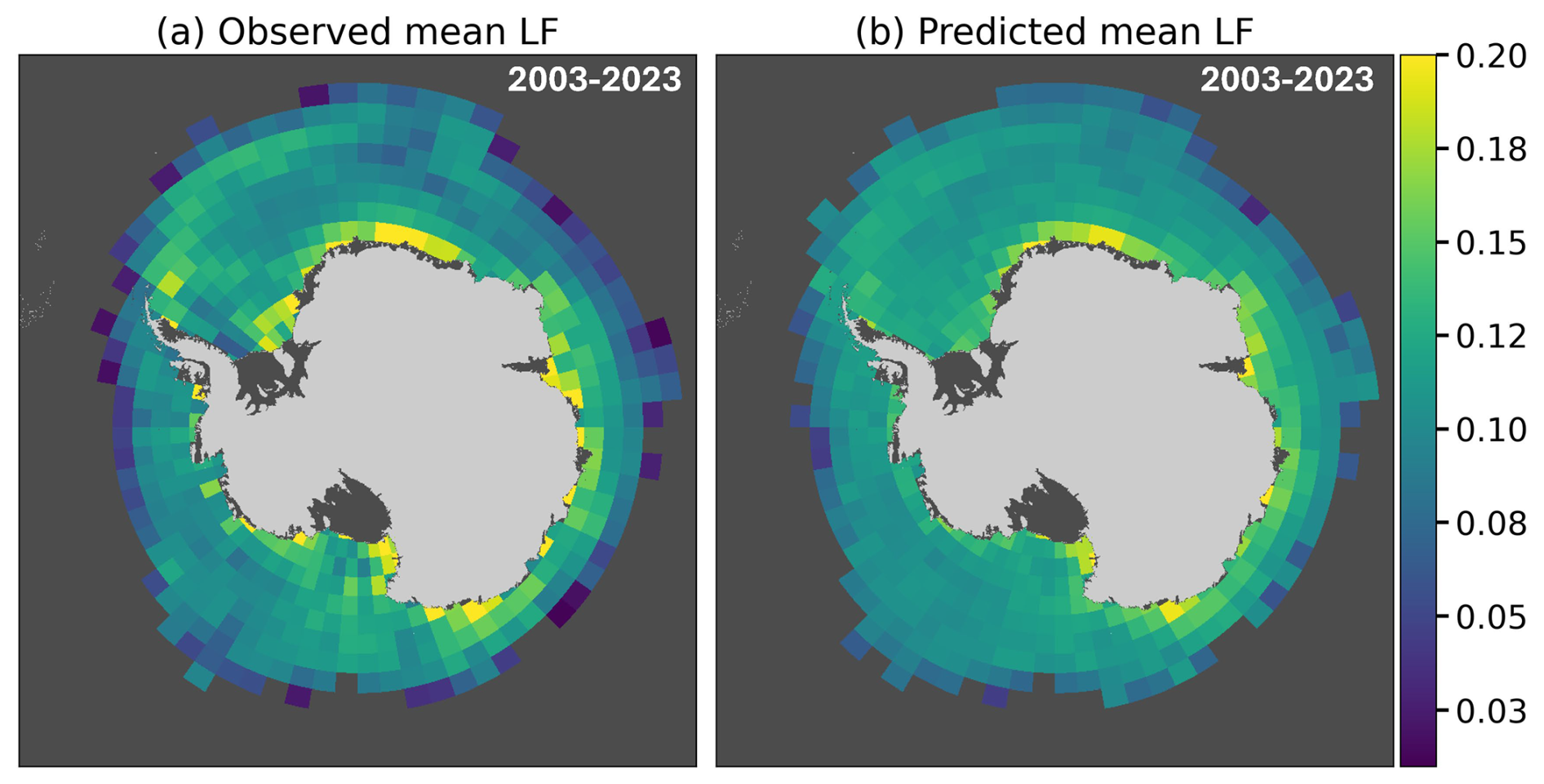
Figure 1 Spatial distribution of (a) observed mean lead frequency and (b) predicted mean lead frequency of the Southern Ocean during the winter period (April–September), 2003–2023, based on the test subset. Data are aggregated to 2° latitude × 5° longitude grid resolution. The colorbar is limited to 0.20 to enhance spatial contrast; values in some coastal regions exceed this threshold.

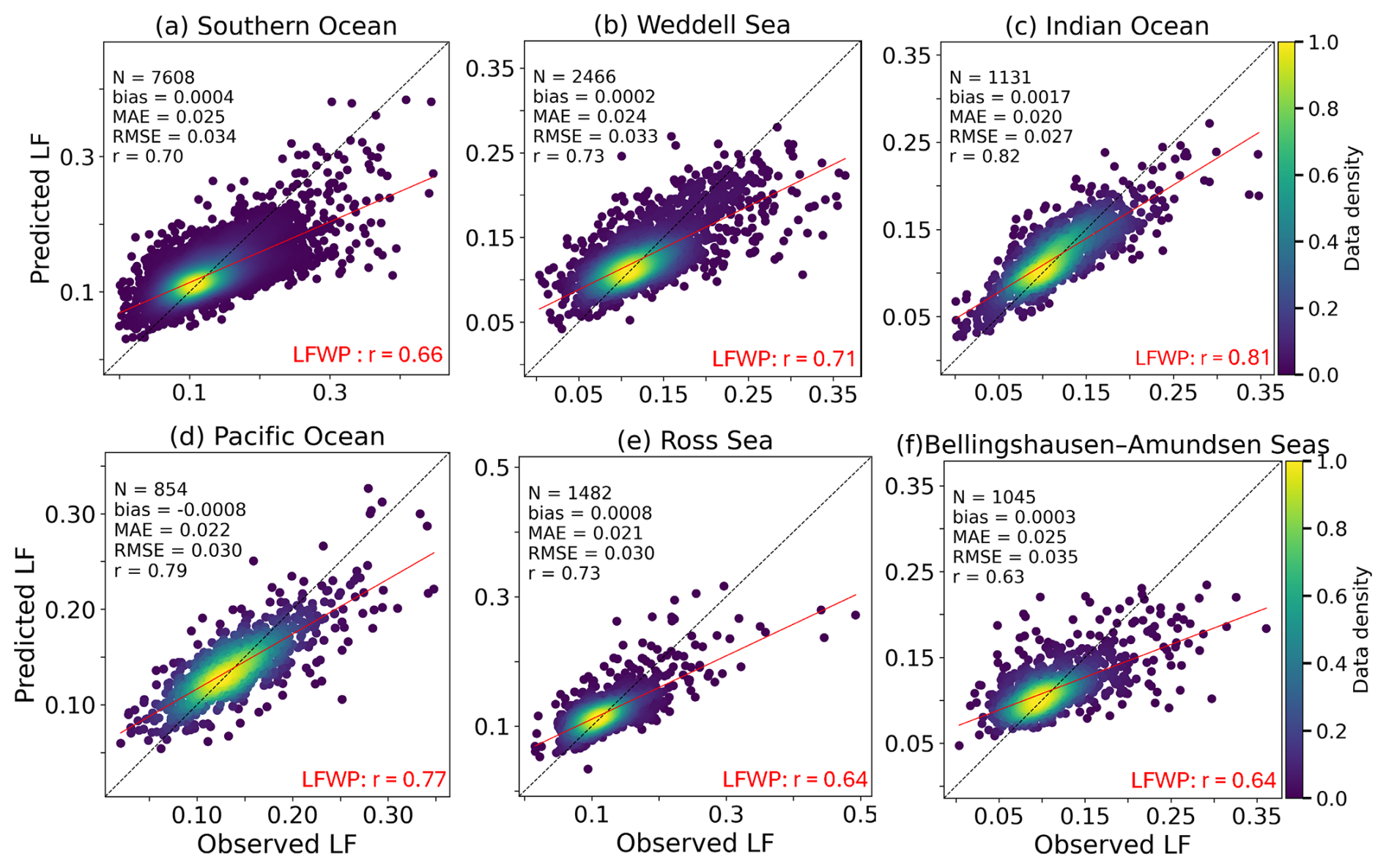
Figure 2 Model performance evaluation comparing observed versus predicted lead frequency based on the test subset for (a) the Southern Ocean and regional sectors: (b) Weddell Sea, (c) Indian Ocean, (d) Pacific Ocean, (e) Ross Sea, and (f) Bellingshausen–Amundsen Seas during April–September, 2003–2023. The black dashed line represents the 1:1 reference line, and the red line shows the linear regression fit. Color gradients indicate data point density. Performance metrics include sample size (N), bias (mean error), mean absolute error (MAE), root mean square error (RMSE), and Pearson correlation coefficient (r), all based on the model with the coastal polynyas from Lin et al. (2024) included. The red text in each panel shows the corresponding r of the model for LF without polynyas (LFWP: r), provided for comparison.

The scatter plot of observed versus predicted LF from the test subset reveals tight clustering around the 1:1 line, particularly for mid-range values between 0.05 and 0.30, suggesting skillful reconstructions for lead frequencies encountered across the Southern Ocean pack ice (Fig. 2a). Density contours in the scatter plots further show that models are more reliable for moderate LF values (0.08–0.20), with a larger spread at both the lowest and highest ends of the distribution. A slight underprediction of strong lead events is evident (LF > 0.20). When evaluated on the test dataset, the model achieved values of r= 0.70, MAE of 0.025, and RMSE of 0.034 for the Southern Ocean in Fig. 2a. For comparison, the model without the inclusion of the polynya dataset (LFWP) achieves r= 0.66 (shown in red) at the pan-Antarctic scale, demonstrating that the representation of coastal polynya activity provides a slight improvement in overall model performance.

Regional validation reveals considerable spatial variability in model performance across the five Southern Ocean sectors (Fig. 2b–f). The Indian Ocean sector shows the highest performance (r= 0.82), followed by the Pacific Ocean (r= 0.79) and the Weddell Sea and Ross Sea (both r= 0.73). The Bellingshausen–Amundsen Seas show the comparatively lowest correlation (r= 0.63). The improvement from including the polynya dataset is most pronounced in the Ross Sea, where r increases from 0.64 to 0.73, and in the Weddell Sea, where r increases from 0.71 to 0.73. In the Indian and Pacific Ocean sectors, the improvement is more modest (r increasing from 0.81 to 0.82 and from 0.77 to 0.79, respectively).

Figure 3 shows that the RF model captures the seasonal evolution of monthly mean LF throughout the winter season, 2003–2023. At the pan-Antarctic scale, predicted monthly LF closely follows observations from April to September, capturing both the timing and magnitude of the rise toward mid-winter and the subsequent late-season decline. Predicted LF increases from April to a June peak near 0.14, before decreasing slightly toward September at lowest LF value (Fig. 3a). Regional temporal evolution shows close agreement across sectors (Fig. 3b–f). The Weddell Sea displays a clear mid-winter maximum, while the Indian Ocean sector shows a gradual decline from April to September, with both observed and predicted values remaining in close agreement throughout winter (Fig. 3c). Seasonal mean LF value gaps are higher between observed and predicted LF in the Pacific sector and in May in the Ross Sea (Fig. 3d–e). The Bellingshausen–Amundsen Seas show the lowest seasonal values in September, and maintain moderate LF values throughout winter (Fig. 3f). Across all sectors, the generally close match between predicted and observed monthly means indicates that the model captures much of the large-scale temporal variability of LF, although noticeable discrepancies remain in some regions and months.

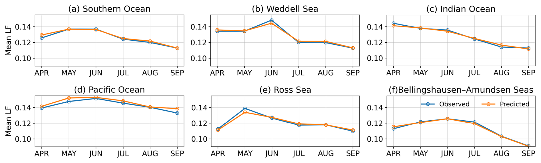
Figure 3 Seasonal evolution of monthly mean lead frequency from April through September, comparing observed (blue) and predicted (orange) values based on the test subset for (a) the Southern Ocean and regional sectors: (b) Weddell Sea, (c) Indian Ocean, (d) Pacific Ocean, (e) Ross Sea, and (f) Bellingshausen–Amundsen Seas during 2003–2023.

3.2 Incremental predictor contribution analysis

Figure 4 presents how different predictor variables contribute to overall model performance based on the test subset. For the Southern Ocean, wind speed alone provides limited skill (r∼0.10), and performance improves steadily as predictors are progressively introduced. The sequential addition of zonal u wind and meridional v wind yields the largest step-gains, raising r to ∼0.45 and ∼0.55, respectively, highlighting the important role of directional wind (zonal u and meridional v winds) forcing in driving lead formation across the Southern Ocean. Ice velocity and ice divergence progressively improve correlation to r∼0.65, ocean current speed to r∼0.68, and the final inclusion of the temporal descriptor (month) brings the correlation to its full value (r= 0.70) at the Southern Ocean scale (Fig. 4a).

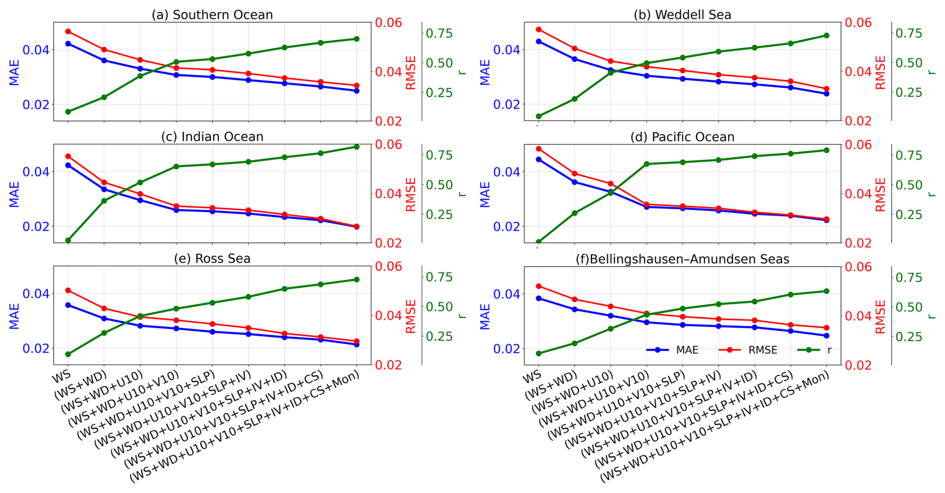
Figure 4 Incremental predictor contribution analysis showing the progressive improvement in model performance as predictor variables are sequentially added for (a) the Southern Ocean and its regions: (b) Weddell Sea, (c) Indian Ocean, (d) Pacific Ocean, (e) Ross Sea, and (f) Bellingshausen–Amundsen Seas during April–September, 2003–2023. Lines represent the MAE (blue), RMSE (red), and r (green). Predictors are added in the following sequence: wind speed (WS) → wind divergence (WD) → zonal u wind (U10) → meridional v wind (V10) → sea-level pressure (SLP) → ice velocity (IV) → ice divergence (ID) → ocean current speed (CS) → month (Mon).

Regions show pronounced differences in how predictor additions affect skill across regions. The Indian Ocean sector (Fig. 4c) demonstrates particularly sharp performance gains from the addition of zonal u and meridional v wind components, with correlation increasing steeply from r∼0.25 after adding wind divergence to r∼0.65 after meridional v wind is included, potentially reflecting the strong directional wind control on lead formation in this sector. The Pacific Ocean (Fig. 4d) shows a similar pattern, ultimately reaching r= 0.79 with the complete predictor set. The Ross Sea (Fig. 4e) shows more gradual improvement throughout the predictor sequence, reaching a final value of r= 0.73. The Bellingshausen–Amundsen Seas (Fig. 4f) show consistent incremental gains across all predictor groups, ultimately reaching r= 0.63 with the full predictor set.

The largest improvements in both correlation and error metrics typically occur when both directional wind components and ocean current speed are introduced, indicating the coupled nature of the atmosphere–ice–ocean system in driving lead variability. While relative importance (Sect. 3.3) quantifies the independent contribution of each predictor in the full model, the incremental analysis reveals the marginal gain of each predictor group and identifies the minimum predictor set required for skillful LF reconstruction.

3.3 Relative importance of predictor variables

Figure 5 summarizes the permutation importance analysis, which reveals the dominant predictors of LF in the RF framework across the Southern Ocean and its regions based on the test sample. At the pan-Antarctic scale, the zonal u wind emerges as the most influential predictor (17.7 %), followed by ocean current speed (13.9 %), wind speed (12.9 %), meridional v wind (12.2 %), and ice divergence (11.2 %). Wind divergence, ice velocity, sea-level pressure, and month provide additional contributions (Fig. 5a).

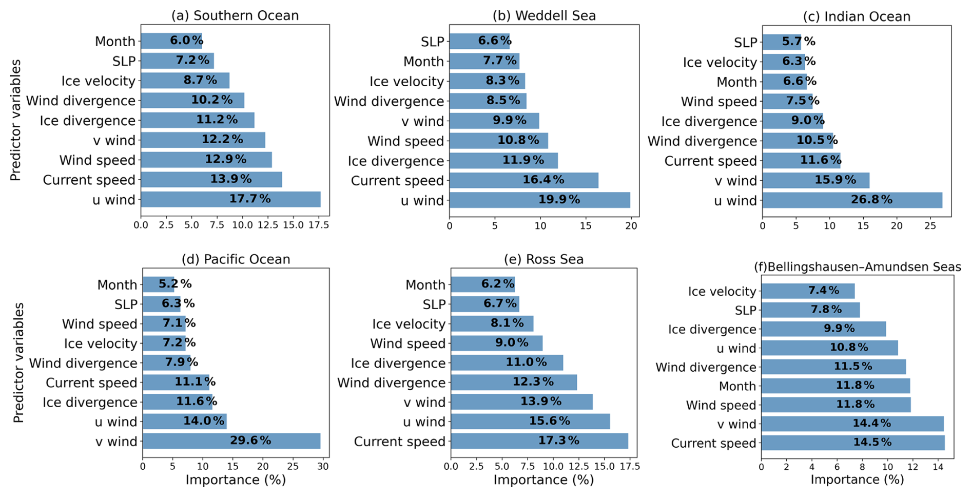
Figure 5 Relative importance of predictor variables for lead frequency based on the test subset across (a) the Southern Ocean and its regions: (b) Weddell Sea, (c) Indian Ocean, (d) Pacific Ocean, (e) Ross Sea, and (f) Bellingshausen–Amundsen Seas during April–September, 2003–2023. Values represent the percentage contribution to the model performance.

Regional importance patterns reveal sector-to-sector differences shown in Fig. 5b–f. The Weddell Sea is dominated by zonal u wind (19.9 %) and ocean current speed (16.4 %), with ice divergence (11.9 %), and wind speed (10.8 %) contributing substantially. The Indian Ocean sector displays the strongest zonal wind control, with zonal u wind accounting for 26.8 % of importance, complemented by meridional v wind (15.9 %), current speed (11.6 %), wind divergence (10.5 %), and ice divergence (9 %). The Pacific Ocean shows meridional v wind influence with 29.6 %, followed by zonal u wind (14 %), ice divergence (11.6 %), and current speed (11.1 %). The Ross Sea exhibits more balanced contributions with current speed (17.3 %), zonal u wind (15.6 %), meridional v wind (13.9 %), wind divergence (12.3 %), and ice divergence (10 %), reflecting its dynamical environment. The Bellingshausen–Amundsen Seas are dominated by ocean currents (14.5 %), with substantial contributions from meridional v wind (14.4 %), wind speed (11.8 %), month (11.8 %), and wind divergence (11.5 %).

Among the predictors at the pan-Antarctic scale, the directional wind components, ocean current speed, and ice divergence show the strongest influences, which point towards the essential roles of atmospheric wind forcing, oceanic traction, and sea-ice deformation in shaping lead and coastal polynya variability (see Sect. 4). Overall, the permutation importance patterns indicate that lead formation arises from coupled non-linear interactions among multiple physical processes rather than from any single dominant predictor, and that the relative importance of these processes varies considerably across the five regional sectors of the Southern Ocean.

3.4 Monthly model performance analysis for winter months

Figure 6 presents the test subset monthly model performance metrics and top-5 predictors for each winter month (April–September, 2003–2023) across the Southern Ocean and regional sectors. The month is excluded as a predictor in this single-month analysis. This demonstrates the monthly and regional evolution of model skill and progressive shifts in predictor dominance throughout the winter.

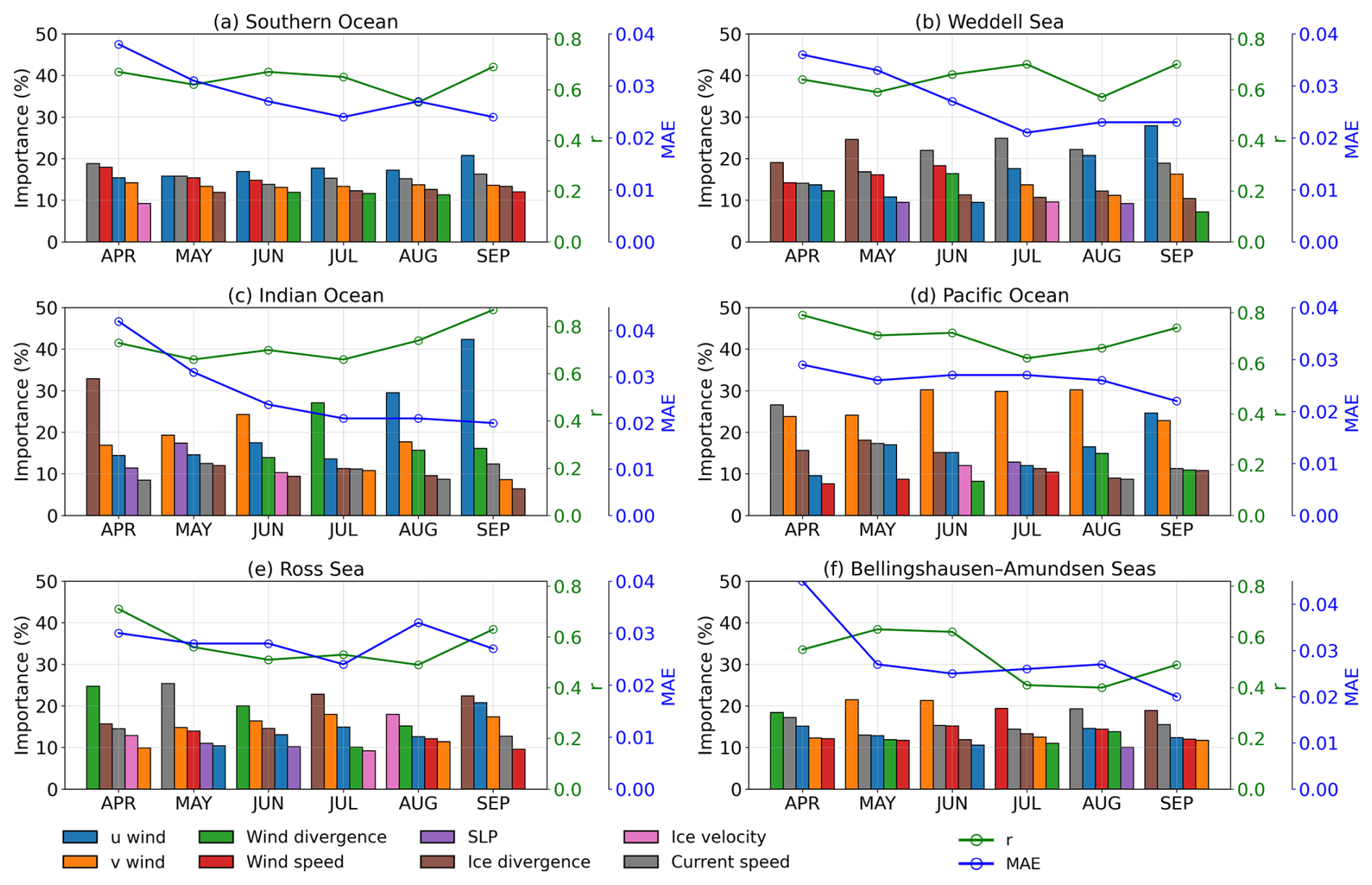
Figure 6 Monthly and regional variation of predictor importance and metrics across Antarctic regions (April–September, 2003–2023). Bar charts show relative importance (%) of top-5 predictors in six Antarctic sectors: (a) Southern Ocean, (b) Weddell Sea, (c) Indian Ocean, (d) Pacific Ocean, (e) Ross Sea, and (f) Bellingshausen–Amundsen Seas. Overlaid lines indicate r (green) and MAE (blue). Predictors include zonal u wind (blue), meridional v wind (orange), wind divergence (green), wind speed (red), SLP (purple), ice divergence (brown), ice velocity (pink), and current speed (grey).

At the pan-Antarctic scale (Fig. 6a), the model performance varies across months, with r ranging between approximately 0.60 and 0.70, with April showing the highest correlation, while August shows comparatively lower skill. The MAE remains relatively stable across months at approximately 0.020–0.030. The dominant predictors show a relatively balanced distribution throughout winter, such as zonal u wind (∼ 18 %–21 %), current speed (∼ 15 %–19 %), and meridional v wind (∼ 13 %–16 %) contributing consistently across all months. Overall, wind field and current speed are higher in importance, indicating a major role of wind-ocean forcing on lead and coastal polynya formation across all winters in the Southern Ocean.

The Weddell Sea (Fig. 6b) exhibits notable seasonal variation in both model skill and predictor importance. In April and May, the model achieves its correlation (r∼0.70 and 0.60), and for both months ice divergence (∼ 20 %–25 %) is the leading contributor. From June to August, current speed increase in prominence as leading drivers, reflecting stronger oceanic forcing during mid-winter. By September, zonal u wind importance rises markedly to approximately 28 %, while the model correlation also recovers to approximately 0.70, indicating stronger zonal u wind control on lead formation in late winter under a thickening ice pack.

The Indian Ocean sector (Fig. 6c) is majorly dominated by v and u winds throughout winter (∼ 15 % in April, rising again to ∼ 42 % in September), while ice divergence in April and wind divergence in July provide primary contributions. Model performance is highest in April and September (r∼0.80), with a slight reduction during mid-winter months. The Pacific Ocean sector (Fig. 6d) shows consistent dominance of meridional v wind accounting for approximately 22 %–31 % of total predictor importance across all months. Model skill remains relatively stable across months (r∼ 0.60–0.75), with the highest correlation in April and September.

The Ross Sea (Fig. 6e) displays more variable predictor importance throughout winter. In April, zonal u wind (∼ 25 %) and current speed (∼ 15 %) are the leading predictors (r∼ 0.75). During May, current speed increases in importance (∼ 25 %), reflecting stronger mechanical deformation during early winter ice consolidation. From June to August, wind divergence and ice divergence together contribute approximately 35 %–40 %, with wind divergence peaking in August (∼ 23 %). By September, ice divergence and zonal u wind regain prominence, suggesting a return to wind-driven control in late winter.

The Bellingshausen–Amundsen Seas (Fig. 6f) show the variable model performance, with r ranging from approximately 0.65 in April to approximately 0.40 in July before recovering slightly toward September. In April, current speed (∼ 19 %), zonal u wind (∼ 18 %), and meridional v wind (∼ 17 %) are the leading predictors. Through May and June, meridional v wind and current speed increase in importance, while from August onward, the predictor importance becomes more evenly distributed among current speed and ice divergence.

Overall, these patterns suggest that lead and coastal polynya formation result from distinct combinations of atmospheric, oceanic, and ice-dynamic physical processes that vary across sectors and evolve throughout the winter season.

3.5 Lead drivers in exemplary sub-regions

To investigate lead and coastal polynya variability and the sensitivity of dominant physical drivers based to regional conditions, we exemplarily identified four coastal regions, shown in Fig. 7, for which the regionally averaged LF was reconstructed from the same predictors as above. These boxes were selected to identify key coastal regions where the model demonstrates statistically significant predictive skill (p<0.05 with r>0.60), and where leads and coastal polynya formation are governed by distinctly different main physical drivers (see Fig. 9). These regions span both the East Antarctic sector (boxes 1–2) and the West Antarctic sector (boxes 3–4), covering the East Weddell coastal zone (box 1, Lazarev Sea), the East Antarctic coastal margin (box 2, D'Urville Sea), the Bellingshausen–Amundsen Seas coast (box 3, Amundsen Sea), and the western Weddell coastal zone (box 4, West Weddell Sea). The observed mean LF for the wintertime period 2003–2023 in these coastal regions is generally high (>0.15), including coastal polynya activity along the Antarctic continental margins (Dubey et al., 2025a; Lin et al., 2024).

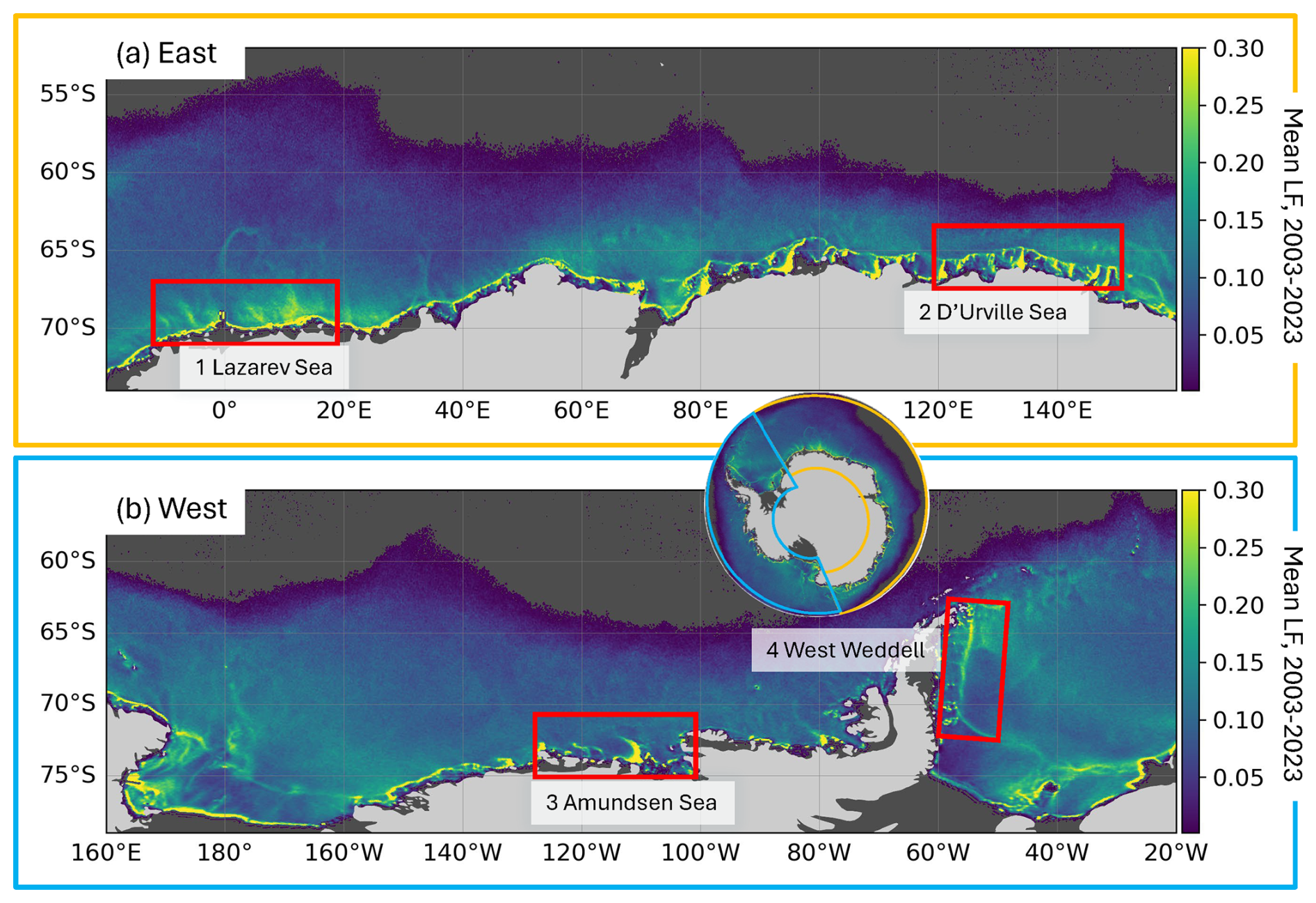
Figure 7 Mean lead frequency (April–September, 2003–2023) for (a) the East and (b) the West Antarctic sectors. Red boxes highlight key coastal regions where the model demonstrates statistically significant predictive skill (p<0.05 and r>0.60), and are used for the local predictor importance analysis in Figs. 8 and 9.

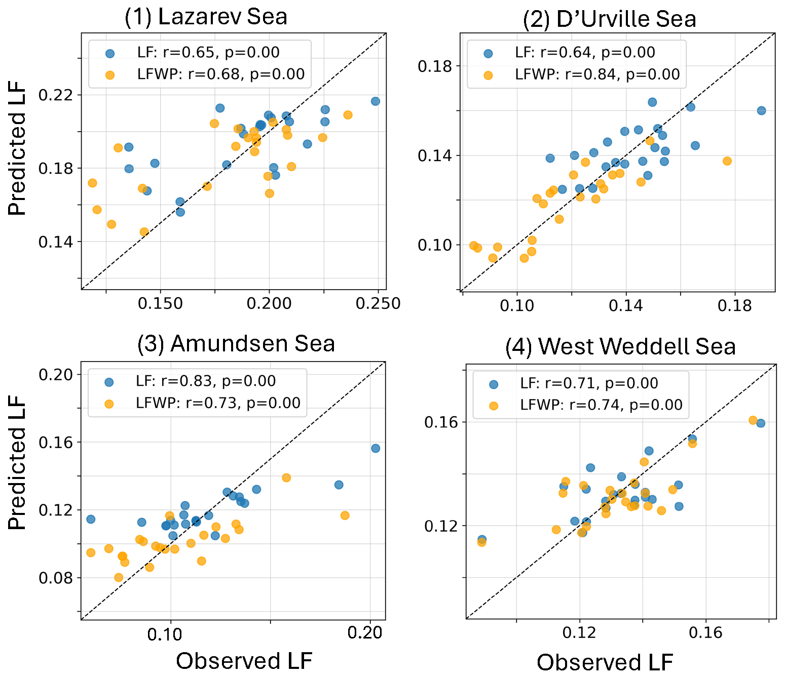
Figure 8 Observed versus predicted monthly mean lead frequency based on the test subset (April–September, 2003–2023) for each of the four coastal boxes identified in Fig. 7. Blue dots (LF) show model performance when the coastal polynyas from Lin et al. (2024) are included, and orange dots (LFWP) show model performance without polynyas.

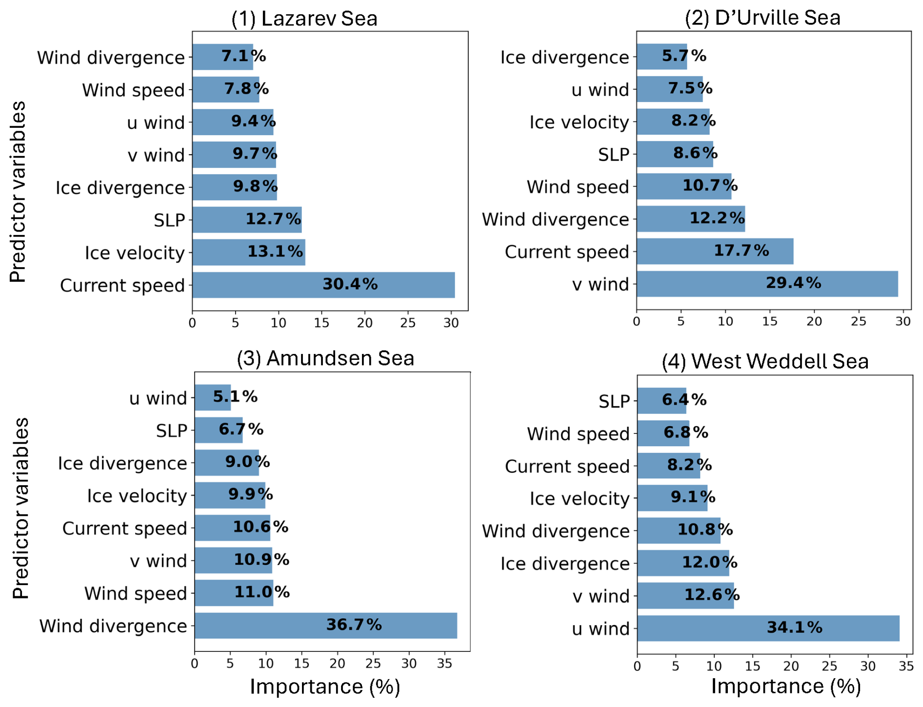
Figure 9 Relative importance of predictor variables for lead frequency based on the test subset (April–September, 2003–2023) for each of the four coastal boxes identified in Fig. 7.

Model performance within the four coastal regions is evaluated in Fig. 8, which shows scatter plots of observed versus predicted monthly mean LF for the period April–September, 2003–2023. Figure 8 shows the model performance when the polynya dataset of Lin et al. (2024) is included (LF, blue dots) and when it is excluded (LFWP, orange dots), allowing a direct assessment of the added value of polynya information in each coastal region. The highest correlation is found in box 3 in the Amundsen Sea (r= 0.83), followed by box 4 in West Weddell Sea (r= 0.71), box 1 along the Lazarev Sea (r= 0.65), and box 2 (r= 0.64) in the D'Urville Sea. Boxes of similar size in the Ross Sea did not provide significant LF reconstruction and are therefore not shown here. However, it must be mentioned that this strongly depends on the location, boundaries, and size of the box.

The comparison between LF and LFWP results reveals regional differences in the added value of the polynya dataset. An improvement is found in box 3, where including the polynya dataset raises r from 0.73 (LFWP) to 0.83 (LF), suggesting that the investigated drivers are well suited to explain polynya activity in this region. In contrast, box 2 in the D'Urville Sea shows a notable decrease from LFWP (r= 0.84) to LF (r= 0.64), indicating that the polynya dataset here rather blurs the connection between predictors and the target variable, and that the pack-ice lead signal already captures the dominant variability in this region. Boxes 1 and 4 show broadly comparable performance with and without the polynya dataset, suggesting that both pack-ice leads and coastal polynyas contribute comparably to the observed LF variability in these regions.

The predictor relative importance analysis for each coastal region (Fig. 9) reveals pronounced spatial heterogeneity in the dominant drivers of coastal lead variability, with each box characterized by a distinctly different main driver (see also Fig. A3). Ocean current speed is the main predictor in box 1 (30.4 %), highlighting a critical role of coastal ocean current dynamics in driving lead formation in this region. In box 2, meridional v wind emerges as the leading driver (29.4 %), indicating that the meridional wind field plays a particularly important role along this section of the Pacific coastal margin, where offshore katabatic winds are likely to drive divergent ice motion and coastal lead formation. Wind divergence is found to be the dominant predictor in box 3 (36.7 %) along the Amundsen Sea coast. Zonal u wind is the dominant predictor in box 4 (34.1 %), reflecting the importance of zonal wind forcing perpendicular to the Antarctic Peninsula in controlling lead opening along the western Weddell Sea coast.

3.6 Coastal influences

The presented results so far indicate that the individual contribution of drivers for lead and coastal polynya formation shows a pronounced spatial variability with a strong dependence on local coastal geometries, as well as distance to coast, distance to marginal ice zone and probably also local bathymetry. To better focus on the effect of coastal distance, Fig. 10 further summarizes the overall RF model skill and dominant predictor importance as a function of distance from the Antarctic coast, across four distance categories (0–50, 50–150, 150–300, and > 300 km). The model correlation in LF is highest in the nearest coastal zone (0–50 km, r= 0.89), where ocean current speed and ice velocity are the leading drivers, and decreases progressively with distance from the coast. Notably, the main and secondary drivers remain consistent across all distance categories for both LF and LPWP except the 50–150 km zone: in the 50–150 km zone, ice divergence becomes the secondary predictor while wind speed emerges as the main predictor for LF, while meridional v wind appears as a co-dominant main predictor for LFWP. In the 150–300 km zone, meridional v wind dominates alongside wind speed as the secondary driver. Beyond 300 km from the coast, ice divergence and ice velocity remain the primary controls, though the overall model correlation drops to approximately r∼ 0.46 for LF. Importantly, almost the same dominant predictors are found for both LF and LFWP dataset, except in the 50–150 km zone, but model skill increases substantially in the nearest coastal zone (Fig. 10), rising from r= 0.73 (LFWP) to r= 0.89 (LF) in the 0–50 km band, while it decreases at larger coastal distances (from r∼ 0.80 (LFWP) to r ∼ 0.62 (LF)) in the 50–150 km band, demonstrating that the representation of coastal polynya activity significantly improves model skill in the regions closest to the Antarctic coastline where polynya and lead dynamics are most tightly coupled whereas model performance decreases as the distance increases from the coast, potentially indicating a lower accuracy of the polynya area data in the pack ice.

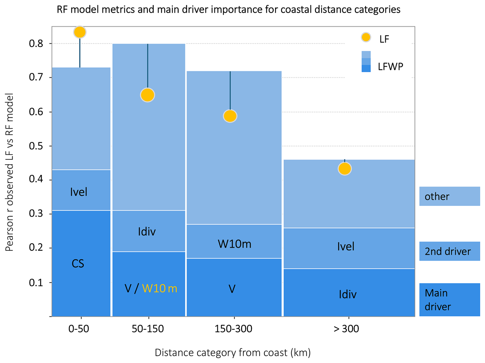
Figure 10 Random-forest model skill and dominant predictor importance as a function of distance from the Antarctic coast, for four distance categories. Stacked bars show the Pearson correlation (r) between observed and predicted lead frequency partitioned among the main driver (dark blue), secondary driver (medium blue), and remaining predictors (light blue), without coastal polynyas (LFWP). Orange dots indicate the model correlation when polynyas identified by Lin et al. (2024) are included (LF). Key predictors are labelled within each bar: current speed (CS), meridional v wind (V), 10 m wind speed (W10m), ice divergence (Idiv), and ice velocity (Ivel).

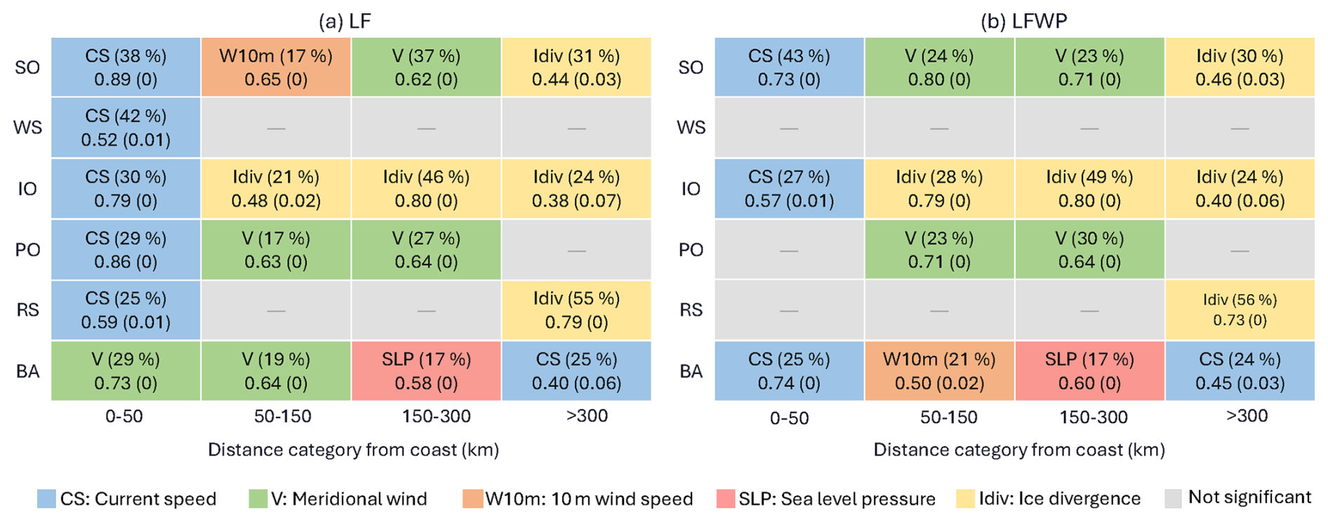
Figure 11 RF model performance and main drivers of (a) LF and (b) LFWP by region and distance from coast. For each region–distance category, the cell lists the main driver and its relative importance (%), followed by the correlation between predicted and observed LF (r) and the associated p-value (p). Grey cells indicate no statistically significant relationship at the 0.1 level. Region: SO – Southern Ocean, WS – Weddell Sea, IO – Indian Ocean, PO – Pacific Ocean, RS – Ross Sea, BA – Bellingshausen–Amundsen Seas.

Figure 11 further extends this analysis by presenting the dominant driver and model performance for each region/distance category combination, for both LF (Fig. 11a) and LFWP (Fig. 11b), with grey cells indicating no statistically significant relationship at the 0.1 level. Regional patterns reveal sector-to-sector variability in both the main drivers and the statistical significance of results across distance categories. In the nearest coastal zone, current speed is the main driver in the Weddell Sea (42 %, r= 0.52), Indian Ocean (30 %, r= 0.79), and Pacific Ocean (29 %, r=  0.86). In the Weddell Sea, no significant relationships are found farther from the coast. In the Indian Ocean, the dominant control shifts from current speed near the coast to ice divergence (21 %–46 %) at larger distances. In the Pacific Ocean, meridional v wind (17 %–27 %) becomes more important at intermediate distances, likely reflecting the influence of offshore winds. In the Ross Sea, significant results appear only in the nearest and outermost distance bands, where current speed (25 %, r= 0.59) near the coast and ice divergence (55 %, r= 0.79) dominate beyond 300 km. The Bellingshausen–Amundsen Seas are the only region where meridional v wind is the main driver close to the coast (29 %), suggesting an important role of offshore wind forcing in this sector.

The dominance of drivers for LF and LFWP is generally similar across most regions and distance bands. The largest difference is found in the nearest coastal zone, where including polynyas improves the model skill at the Southern Ocean scale in the 0–50 km band. In the Bellingshausen–Amundsen Seas, the dominant driver also changes from meridional v wind in LF to current speed in LFWP. This suggests that the pack-ice lead activity in this region is more strongly linked to ocean currents, whereas offshore winds play a larger role in controlling lead and coastal polynya variability.

4 Discussion

The presented results indicate that the individual contributions of drivers for lead and coastal polynya formation show a pronounced spatial variability with an apparent strong dependence on factors such as local coastal geometries, distance to coast, distance to marginal ice zone and probably also local bathymetry. While a pan-Antarctic quantification of driver importances shows the zonal u wind component to have the strongest contribution to lead variability (Fig. 5), ocean current speed dominates the lead variability close to the coast (0–50 km distance, Fig. 10). Extending the LF data set by polynya areas explicitly improves the reconstruction skill of the model overall, but with a notable effect only close to the coast. The model achieves r= 0.70 at the pan-Antarctic scale, indicating that the used predictors capture a substantial fraction of LF variability. A notable portion of LF variance remains unexplained, reflecting both unresolved processes and limitations that arise from temporal resolution. In consequence, this highlights the need for high-resolution lead-resolving modelling to better understand ocean–ice–atmosphere interactions in bathymetrically-controlled and coastal lead zones.

Atmospheric forcing variables collectively represent the largest contribution to model skill. The zonal u wind component accounts for 17.7 % of the explained variance in LF across the Southern Ocean, reaching as high as 26.8 % in the Indian Ocean sector and 19.9 % in the Weddell Sea (Fig. 5). Together, zonal u and meridional v wind components collectively contribute approximately 30 % of the total relative importance at the pan-Antarctic scale, underscoring the fundamental role of directional wind forcing in driving lead formation across the Southern Ocean. The dominance of the wind components reflects the well-established link between near-surface wind forcing and mechanical ice divergence, whereby divergent wind stress promotes tensile failure in the ice cover by weakening internal ice strength and enhancing shear deformation (Simmonds et al., 2008; Kimura and Wakatsuchi, 2000). The monthly analysis (Fig. 6) reveals that atmospheric wind forcing is prominent throughout winter across all sectors. At the pan-Antarctic scale, zonal u wind (∼ 18 %–21 %) and meridional v wind (∼ 13 %–16 %) contribute consistently across all months, indicating a major role of wind forcing on lead formation across seasons. The Indian Ocean sector is dominated by v and u winds throughout winter, together rising to ∼ 42 % by September, reflecting the persistent influence of zonal wind (Heil and Allison, 1999). The Pacific Ocean sector shows consistent dominance of meridional wind (∼ 22 %–31 %) across all months, reflecting the strong meridional wind control imposed by the Amundsen Sea Low (Turner et al., 2017; Meehl et al., 2019). In the Ross Sea, wind divergence peaks in August (∼ 23 %), consistent with the intense episodic offshore wind events characteristic of this sector (Mathiot et al., 2012; Silvano et al., 2018). The exemplary coastal boxes analyzed in Sect. 3.5 further illustrate the heterogeneous nature of wind-driven lead and coastal polynya formation at the local scale (see Figs. 9 and A2). While zonal wind dominates lead and coastal polynya opening in the West Weddell Sea, meridional wind controls LF along the D'Urville Sea coast, where offshore katabatic winds draining from the Antarctic ice sheet are likely to drive divergent ice motion and coastal lead formation in both coastal regions.

Ice velocity and ice divergence provide additional model skill, contributing about 20 % to overall model performance (Fig. 5a). Ice divergence alone contributes 11.2 %, while ice velocity adds 8.7 %. Despite this performance, the importance of ice predictors, along with their regional contrasts (Fig. 5), is consistent with the well-established link between deformation processes and lead formation. The Weddell Sea shows relatively high ice kinematic importance, with ice divergence contributing 11.9 % and ice velocity 8.3 %, in line with its persistent Weddell Gyre and shear zones and characteristic cyclonic drift patterns (Hoeber, 1991). In contrast, the Ross Sea shows an ice kinematic importance with ice divergence (11.0 %) and ice velocity (8.1 %) contributing alongside the dominant wind and ocean current predictors (Fig. 5), likely reflecting the Ross Gyre and hence higher LF variability.

The distance-from-coast analysis (Fig. 10) reveals that ice kinematic predictors play an increasingly important role in the offshore pack ice. Beyond 300 km from the coast, ice divergence and ice velocity emerge as the primary controls on lead variability, while ocean current speed and wind components become comparatively less dominant. This transition reflects the changing balance between wind-driven and ice-dynamic forcing across the Southern Ocean, with the offshore pack ice responding more to accumulated internal stress and long-term deformation patterns rather than the episodic wind events and coastal boundary effects that dominate the nearshore environment (Hutchings et al., 2011; Holland and Kwok, 2012). The regional results shown in Fig. 11 support this transition. Ice divergence becomes the main driver beyond 300 km in the Indian Ocean and Ross Sea, while current speed and wind components remain more influential at shorter coastal distances. This highlights the different physical main drivers controlling the LF between the nearshore region and the offshore pack ice.

Ocean current speed remains a consistent co-dominant predictor throughout winter at the pan-Antarctic scale (Fig. 6). In the Weddell Sea, current speed increases in prominence from June to August as a leading driver, reflecting stronger oceanic forcing during mid-winter, probably associated with the Weddell Gyre circulation (Haumann et al., 2016; Cheon et al., 2014). The Ross Sea shows current speed importance rising markedly in May (∼ 25 %). In the Bellingshausen–Amundsen Seas, current speed leads in April (∼ 19 %) before becoming a major driver in August, reflecting the region's persistent sensitivity to oceanic forcing throughout winter, together with winds. This seasonal evolution across all sectors points towards a growing role of sustained bathymetrically guided flows and intensified ice–ocean coupling beneath thickened ice as winter progresses, where lead formation becomes increasingly controlled by persistent ocean-driven shear alongside wind forcing (Leng et al., 2024; Stewart et al., 2019). The regional and distance-dependent driver patterns summarized in Fig. 11 shows that current speed is the primary control in the nearest coastal zone (0–50 km) across most sectors, except for the Bellingshausen–Amundsen Seas, where meridional v wind rather than current speed dominates in the nearest coastal zone, suggesting that offshore winds, acting as a strong southerly meridional forcing, play a particularly important role in driving divergent ice motion and lead opening along this coastline (Mathiot et al., 2012).

The consistency of directional wind component importance across all regions (collectively ∼ 25 %–43 %), combined with marked regional variations in secondary predictors, indicates that directional wind forcing is fundamental while oceanic and ice-dynamic forcings provide region-specific modulations.

Large-scale climate modes such as the Southern Annular Mode (SAM), El Niño–Southern Oscillation (ENSO), and the Indian Ocean Dipole (IOD) are well known to shape Antarctic sea-ice extent and the position of the marginal ice zone by modulating atmospheric circulation, wind fields, and ocean currents (Hall and Visbeck, 2002; Yuan, 2004; Blanchard-Wrigglesworth et al., 2021). These same processes are likely to influence the sea-ice leads and coastal polynyas by altering patterns of divergence and ice drift. When considering LF trends, the atmosphere is usually seen as the dominant driver, while the ocean largely determines how those trends vary from season to season over the years (Holland and Kwok, 2012; Hobbs et al., 2016). Understanding the connection between lead variability, coastal polynya activity, short-lived atmospheric events, and slow, pan-Antarctic scale climate shifts including climate modes therefore remains an important avenue for future work, particularly in the context of the variability observed in Antarctic sea-ice since 2016.

A further avenue for improvement is to explicitly account for the circum-Antarctic landfast ice regime in which many coastal leads and polynyas are embedded. Fraser et al. (2020) provide a pan-Antarctic fast-ice dataset for 2000–2018, and Fraser et al. (2021) identified eight regional fast-ice regimes with distinct trends driven by bathymetry and grounded icebergs. Incorporating fast-ice extent or persistence from these products in our RF framework could help to better distinguish coastal dynamical regimes and to explain part of the residual variance in LF along the Antarctic margins.

Beyond landfast ice, both the target variable and predictor fields carry some limitations that may limit model performance. Among predictors, ORAS5 surface currents are likely subject to uncertainties in the thin, seasonally ice-covered coastal ocean, where observational constraints are sparse and small-scale bathymetric features, tides and mixing are not fully resolved in the reanalysis (Zuo et al., 2019). A limitation of our coastal analysis can be the use of ORAS5 ocean surface current speed as a predictor in the Antarctic shelf and slope regions. ORAS5 is a global, 0.25° ocean reanalysis designed for basin-scale applications, and its resolution and observational constraints may not be sufficient to fully resolve shelf break dynamics and the Antarctic Slope Current (ASC). While permutation importance indicates that ORAS5 contributes substantially to predictive skill, the dataset's own uncertainties are not propagated through the importance estimation, and future work using ensemble realizations or alternative independent products would help quantify how sensitive this ranking is to input-data uncertainty. Future studies could explore alternative products such as the Biogeochemical Southern Ocean State Estimate (B-SOSE; Verdy and Mazloff, 2017), which provides higher-resolution (∼ 18 km) estimates of Southern Ocean circulation. Additional oceanic predictors, such as ocean current divergence and eddy kinetic energy, represent an important objective for future studies, particularly in regions of rough topography and at shelf breaks where the model currently shows comparatively lower skill.

5 Conclusions

This study provides a quantitative assessment of the physical drivers governing wintertime Southern Ocean leads and coastal polynyas activity using an RF regression framework. By combining a 20-year gap-filled satellite-derived LF dataset with a coastal polynya dataset, along with atmospheric, sea-ice, and oceanic predictor variables, we identify and rank the processes controlling lead and coastal polynya formation across the Southern Ocean and five regional sectors. The overall winter model reconstructs the observed LF over the April–September period from 2003 to 2023, achieving a basin-wide correlation of 0.70 between observed and predicted LF values on an independent test dataset.

Permutation-based relative importance analysis reveals a ranking of LF drivers that shows dependencies on region, ice regime and distance to the coast. The directional wind components together contribute approximately 30 % at the pan-Antarctic scale, underscoring the fundamental role of zonal and meridional wind forcing in driving mechanical ice divergence and lead opening across the Southern Ocean. Wind speed, ice divergence and ocean current speed each contribute ∼ 11 %–14 %, suggesting that lead and coastal polynya formation is governed by coupled atmosphere-ice-ocean interactions rather than by any individual main process. Regional analyses further underscore the heterogeneous nature of Southern Ocean lead dynamics. The Indian and Pacific Ocean sectors are dominated by directional wind forcing (zonal u wind: 26.8 % and meridional v wind: 29.6 % respectively), while the Weddell Sea shows a mechanical influence from zonal u wind, ocean currents and ice divergence. The Ross Sea reflects contributions from ocean current speed, directional winds and wind divergence, and the Bellingshausen–Amundsen Seas show predictor importance with ocean current speed and meridional wind leading.

The presented results indicate that the individual contribution of drivers for lead formation shows a pronounced spatial variability with a strong dependence on local coastal geometries, as well as distance to coast, distance to marginal ice zone and probably also local bathymetry. The coastal analysis shows that ocean current speed dominates in the nearest coastal zones (0–50 km), while wind components and ice divergence control lead variability further offshore. The inclusion of the Lin et al. (2024) polynya dataset improves model skill in the nearest coastal zones, with correlation increasing from approximately 0.73 to 0.89 in the 0–50 km band.

The RF model provides a quantitative ranking of LF predictors. Our results show that Southern Ocean lead and coastal polynya formation arise from coupled, non-linear interactions among the atmosphere, ocean, and sea-ice. The presented framework offers a new insight for future work, linking lead and coastal polynya variability to large-scale forcing and climate modes and may provide impetus for improving lead-related fluxes under changing Antarctic sea-ice conditions.

Appendix A

A1 Southern Ocean regional sectors for LF analysis

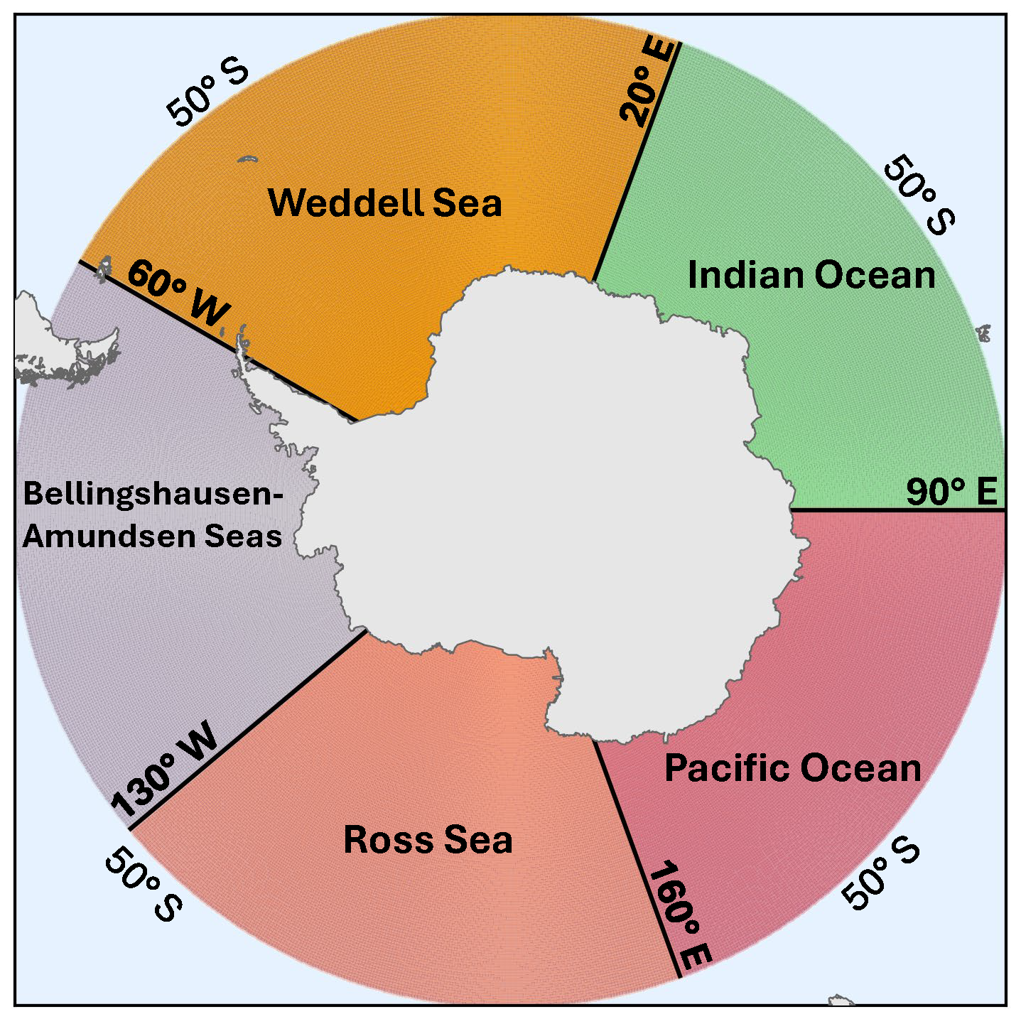
Figure A1 Map of the Southern Ocean showing the five regional sectors used in this study: Weddell Sea (orange), Indian Ocean (green), Pacific Ocean (pink), Ross Sea (coral), and Bellingshausen–Amundsen Seas (grey). The sectors are defined by meridional longitude boundaries, and major latitude circles (50° S) are shown for geographic reference.

A2 Spatial distribution of model bias

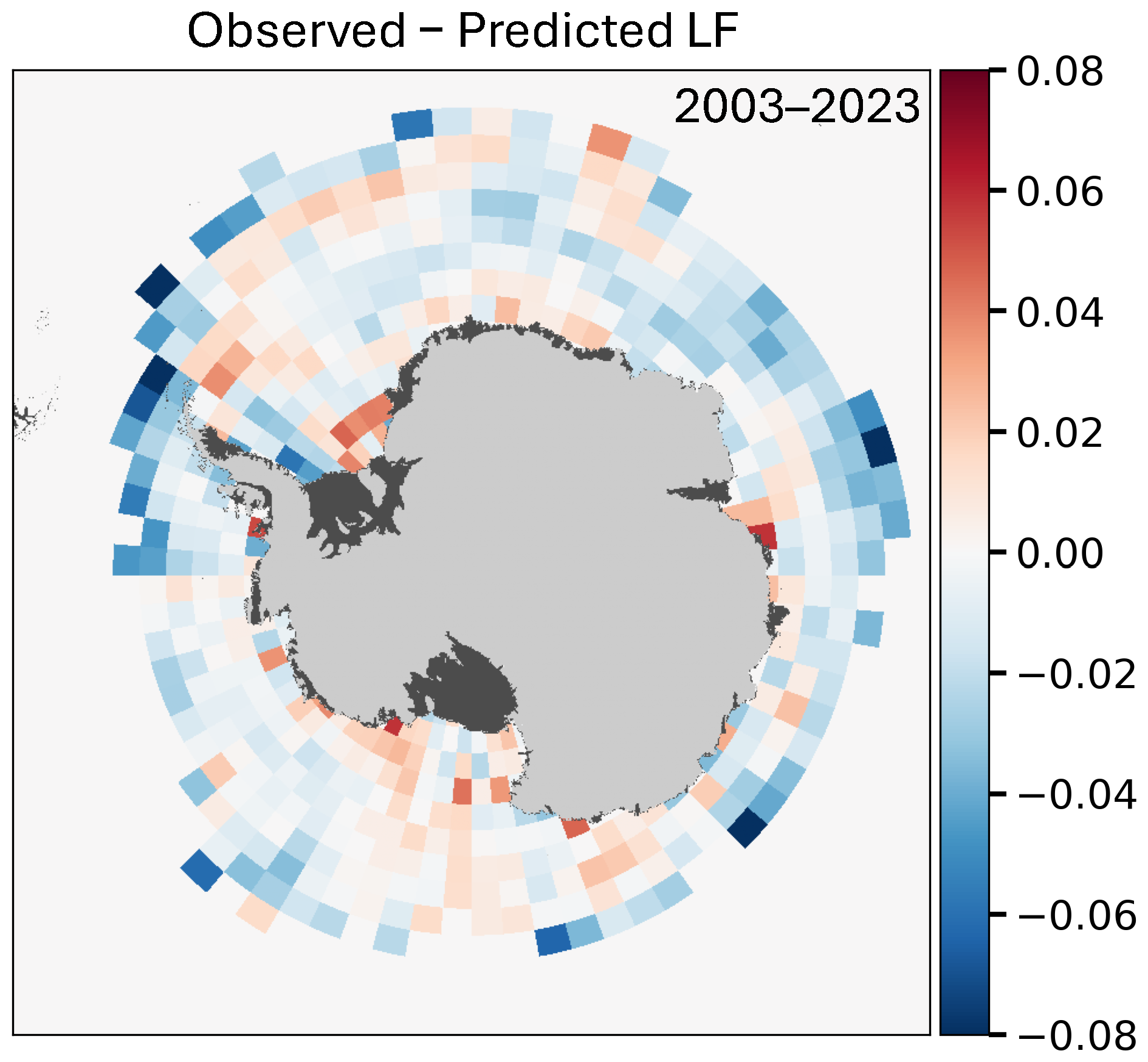
Figure A2 Spatial difference between observed and predicted mean LF (Observed – Predicted LF) for the Southern Ocean from April to September, 2003–2023, based on the test subset. Data are aggregated to 2° latitude × 5° longitude grid resolution, consistent with Fig. 1.

A3 Mean fields of predictor variables

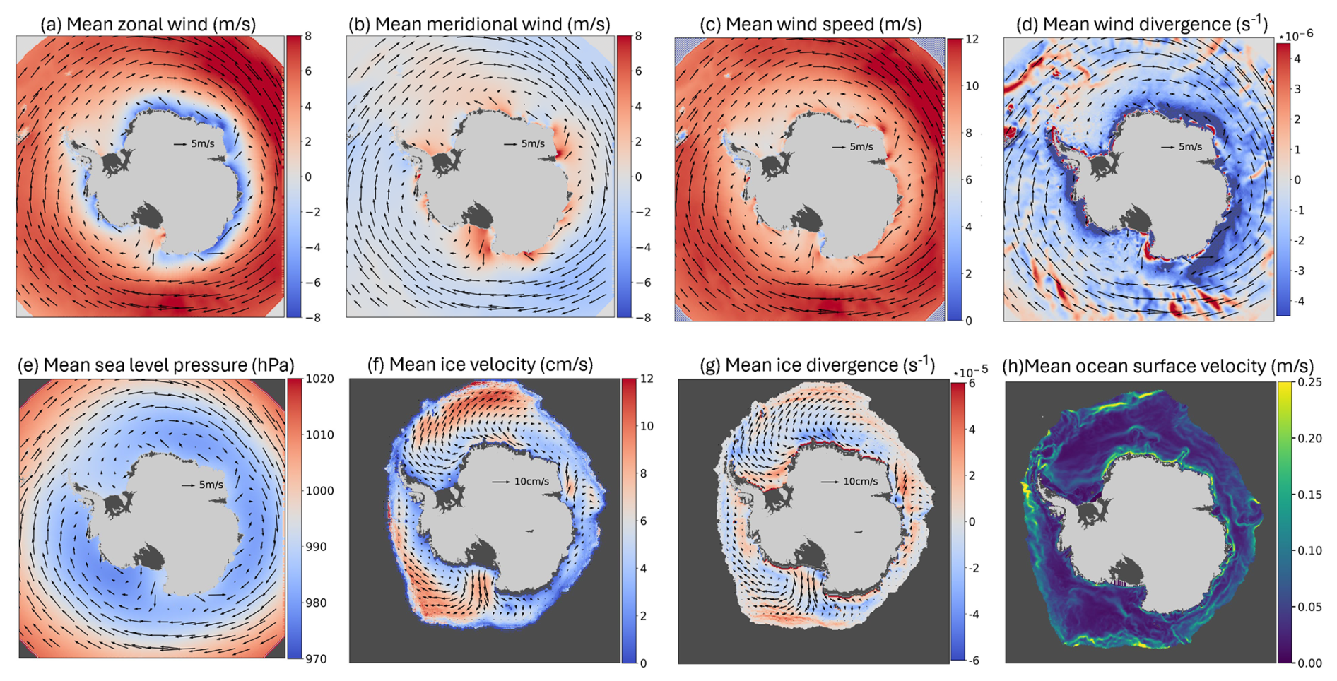
Figure A3 Mean winter (April–September, 2003–2023, excluding 2012) fields of predictor variables used for LF analysis: (a) 10 m zonal u wind, (b) 10 m meridional v wind,(c) 10 m wind speed, (d) wind divergence, (e) sea level pressure, (f) ice velocity, (g) ice divergence, and (h) ocean surface current speed. Mean wind vectors (5 m s⁻¹) and mean ice motion vectors (10 cm s⁻¹) are shown as black arrows in the respective panels. All atmospheric fields are from ERA5, ice motion from the Polar Pathfinder product, and ocean currents from ORAS5. ERA5 data © Copernicus Climate Change Service (C3S), ECMWF. Polar Pathfinder ice motion data © NSIDC. ORAS5 ocean reanalysis data © ECMWF.