Contrasting dynamics of lake- and marine-terminating glaciers under same climatic conditions

In Greenland, mass wasting through frontal ablation occurs not only at the ice-ocean interface but also at the ice-lake intersection. Recent studies have found that lakes cover 10 % of the entire ice sheet margin and stress the importance of understanding frontal dynamics in lacustrine settings. However, relatively little is known about how lake-terminating glaciers compare to marine-terminating glaciers under the same climatic conditions. At a unique study site in South Greenland, a lake and a marine terminus are part of the same glacier system (Qooqqup Sermia), subject to the same regional climate forcings and fed by the same upstream ice masses. In this study, we analyse the drivers of change at both glacier fronts and compare their dynamics with a comprehensive remote sensing dataset supported by climate model output. Furthermore, during two field campaigns, we collected lake bathymetry data alongside temperature and lake level measurements. We find that despite being subject to the same regional climate forcing and fed by the same upstream ice masses, the two termini show contrasting front dynamics in the long- and short-term. We infer extremely low subaqueous melt rates in the lake as one of the main differences between the two environments, likely contributing to the observed contrast in dynamics. A massive disintegration event of more than 3 km of the lake terminus showcases the possibility of rapid mass loss at lake-terminating glaciers in Greenland. Our results stress that lake- and marine-terminating glaciers require separate estimates of frontal ablation through subaqueous melt when included in model simulations of the Greenland Ice Sheet.

1 Introduction

The Greenland Ice Sheet (GrIS) is one of the largest contributors to contemporary sea level rise (Fox-Kemper et al., 2021). Its mass loss is partitioned by surface melt and dynamic ice discharge into the ocean through calving and submarine melt (Mouginot et al., 2019; Otosaka et al., 2023). Both modes of mass loss have increased strongly in the 21st century (Shepherd et al., 2020) as a consequence of higher air temperatures (Hanna et al., 2012) and warm ocean water (Straneo and Heimbach, 2013; Wood et al., 2021). Future projections of mass loss from Greenland vary strongly between different models and climate scenarios (Goelzer et al., 2020), with one of the largest uncertainty arising from the difficulty in resolving the frontal dynamics of tidewater glaciers. At the ice-ocean boundary, ice is rapidly lost through iceberg calving and submarine melt (Benn et al., 2007; Truffer and Motyka, 2016), which can alter the force balance and consequently trigger a speed up of glacier flow, resulting in a higher dynamic mass loss (Joughin et al., 2008; Nick et al., 2009). Calving and submarine melt are complex processes that are strongly influenced by the characteristics of the terminal environment, such as ocean temperature (Wood et al., 2021), tides (Holmes et al., 2023), wave action (Pȩtlicki et al., 2015), plume formation (Cook et al., 2021), and buttressing through an ice mélange (Barnett et al., 2023; Wehrlé et al., 2023).

These complex interactions of ice and water are not unique to marine settings, but also occur in lacustrine settings, potentially further increasing dynamic ice loss in Greenland. Recent studies have identified a large number of ice-marginal lakes with more than 2300 occurrences larger than 0.05 km² (How et al., 2021). Together, these lakes constitute 10 % of the total GrIS margin (up to 26 % regionally) and accelerate ice flow velocities and margin retreat, compared to the land-terminating sections of the ice sheet (Mallalieu et al., 2021; Carrivick et al., 2022). Furthermore, the number of ice-marginal lakes and their impact on the GrIS is expected to grow as the ice sheet recession continues. Carrivick et al. (2022) identified thousands of over-deepenings that, upon retreat, could transform into ice-marginal lakes. A study of central and southwestern Greenland showed a notable 44 % increase in lakes between 1987 and 2010 (Carrivick and Quincey, 2014).

Lake-terminating glaciers are generally known to have lower flow velocities and ice discharge compared to marine-terminating glaciers in Greenland (Mallalieu et al., 2021; Carrivick et al., 2022). However, it is unclear which processes control their dynamics at the terminus in detail. Furthermore, a comparison of the two different terminal environments under the same climatic conditions is lacking.

In South Greenland, a unique study site poses the possibility of conducting such a comparison. At Qooqqup Sermia, both a marine and lake terminus are part of the same glacier system, subject to the same climatic forcings, fed by the same upstream ice masses and also comparable in size. Despite its uniqueness, research on the glacier system is limited to early descriptions from Weidick (1959, 1963) and Warren and Glasser (1992). Weidick summarises earlier expeditions to the region and notes that no reliable glacier positions can be inferred from their reports. Almost thirty years later, Warren and Glasser describe a non-linear response of the glacier termini to climate warming. In addition, there are paleoglaciological studies mapping and dating late Holocene moraines of the Qoqquup Sermia system (maximum Holocene extent about 1.5 ka BP) (Bennike and Sparrenbom, 2007; Winsor et al., 2014) and a reconstruction of paleo ice thickness (Puleo and Axford, 2023).

This study aims to compare glacier dynamics at the marine- and lake-terminating glacier and to discuss drivers of differences between the two environments. To achieve this, we used a combination of field observations, remote sensing, and climate model data. We compiled a dataset consisting of margin outlines, surface velocities, elevation changes, lake ice cover, surface runoff, lake temperature, and lake bathymetry. To put our findings into context, we also describe the general characteristics and historical evolution of Qooqqup Sermia. Our findings suggest that lake- and marine-terminating glaciers need separate estimates of frontal ablation through subaqueous melt when included in model simulations.

2 The Qooqqup Sermia system: a unique study site in South Greenland

The Qooqqup Sermia system is located close to the town of Narsarsuaq in South Greenland (Fig. 1). The glacier system drains a catchment of approximately 2400 km² (Mouginot and Rignot, 2019) and has three major outlet glaciers: Kiattuut Sermiat terminating on land, Qooqqup Sermia terminating in the Qooroq Fjord, and an unnamed glacier, which splits from Qooqqup Sermia and flows into Lake Motzfeldt. In the following, we refer to the tidewater glacier as the Marine Terminus (MT) and to the glacier flowing into Lake Motzfeldt as the Lake Terminus (LT).

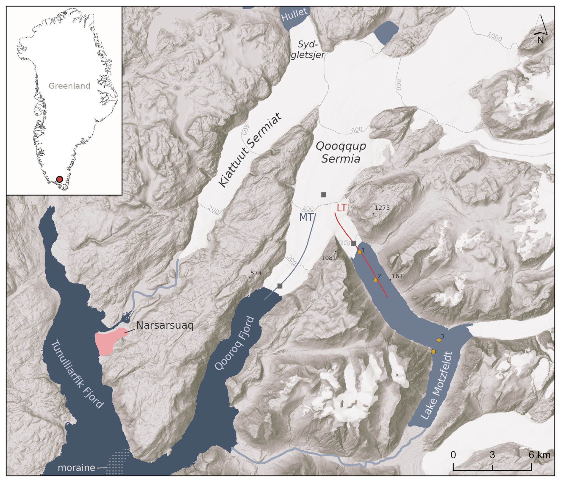
Figure 1 Map of the study area. The blue (MT) and red (LT) lines indicate the elevation profiles used in this study. The grey squares indicate locations for which we show ice surface velocity. Yellow circles indicate CTD profiles with the respective number. The yellow pentagon shows the location of the temperature-depth sensor. The hillshade is based on the ArcticDEM (Porter et al., 2023).

The marine terminus is about 1.7 km wide and the glacier front reaches heights up to 65 m above water (based on UAV field surveys in August 2024). The water depth directly at the glacier front is unknown. However, at approximately 3 km from the current glacier front, the fjord has a depth of 350–375 m (OMG, 2019). With increasing distance from the glacier, the fjord deepens to ∼ 480 m before becoming more shallow again toward the fjord mouth. The fjord mouth is characterised by a large Holocene submarine moraine (less than 50 m water depth at one location), which prevents larger icebergs from exiting into the adjacent Tunulliarfik fjord (Vorndran and Sommerhoff, 1974; Weidick, 1963).

The lake terminus is currently about 1.6 km wide and has a glacier front height of up to 30 m above lake level (based on UAV field surveys in August 2024). Lake Motzfeldt is approximately 15 km long and 2 km wide and lies at an elevation of 160 m above sea level. Besides the lake terminus of Qooqqup Sermia, a second, unnamed glacier flows into the lake on the eastern side. Throughout the year, the lake is covered with several large tabular icebergs (> 0.1 km²) and many smaller icebergs (visible in Fig. 2).

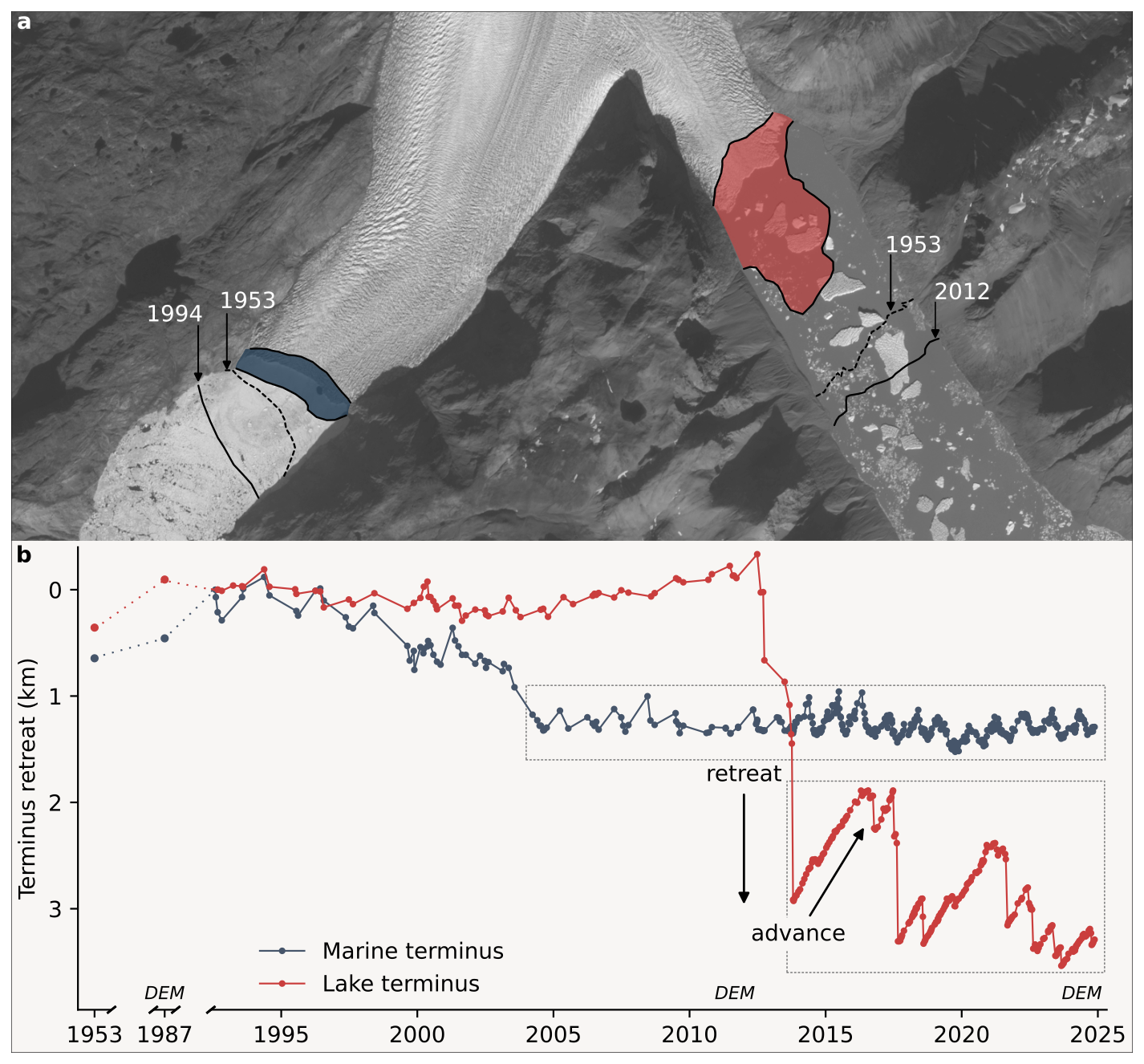
Figure 2 Terminus positions of the marine terminus (left, blue) and the lake terminus (right, red). Panel (a) shows the earliest observations in 1953, the maximum positions in 1994 (MT) and 2012 (LT), and the areas of advance and retreat (blue and red shaded areas). The shading is bound by the local maximum and minimum positions after the respective retreat in 2004 and 2012. Background: Copernicus Sentinel-2 image from 19 September 2024. Panel (b) shows the terminus retreat relative to the first satellite observations in 1992. The dotted boxes indicate the period for the shading in panel (a). Years with available digital elevation models are marked above the x-axis.

The closest weather station to MT and LT is located at the Narsarsuaq airport. At this station, the mean annual air temperature (MAAT) between 1981 and 2010 was 1.1 °C (Drost Jensen, 2025). During the last 15 years (2010–2024) the MAAT was more than 1 °C higher with an average of 2.2 °C. Mean monthly temperatures are lowest in February (−7.4 °C ) and highest in July (10.8 °C).

3 Methods

To understand the dynamics and drivers of change at the marine and the lacustrine glacier margin, we used a combination of remote sensing, field methods, and analysis of climate model data. Specifically, we used remote sensing data to outline glacier front positions, measure surface elevation changes, ice flow velocities and to identify lake ice duration. In the field, we conducted a bathymetric survey of Lake Motzfeldt alongside temperature and lake level measurements during two field campaigns in 2024 and 2025. Furthermore, we used the output of the regional climate model RACMO.

3.1 Glacier front positions

We manually outlined glacier front positions for the marine- and the lake-terminating glacier based on optical satellite images from Landsat 4, 5, 7 and 8 for the period 1992–2024. The images were downloaded using Google Earth Engine, and the margins were digitised using ArcGIS Pro. For Landsat 4 and 5, we used the near-infrared band (band 4) at a spatial resolution of 30 m. For Landsat 7 and 8, we used the panchromatic band (band 8), with a spatial resolution of 15 m. We identified additional front positions for 1987 based on orthorectified 2 m aerial images (Korsgaard et al., 2016) and for 1953 based on aerial images from The Danish Agency of Climate Data. The 1953 images were manually georeferenced based on tie points. We outlined a total of 389 and 308 front positions for MT and LT, respectively. While Landsat 4, 5 and 7 images only allowed for a relatively sparse temporal resolution with about 3–5 images per year, cloud-free Landsat 8 images were available on average every 15 (MT) and 17 d (LT), allowing for a seasonal analysis over the 11 years from 2014 to 2024. We quantified relative changes in the terminus positions using the variable box method as implemented in the Margin change Quantification Tool (MaQiT) (Lea, 2018). By considering the entire width of the glacier terminus, the method allows the detection of uneven changes along the glacier front. For the lake terminus, we identify major calving events by extracting glacier front position changes larger than 50 m between two images. Since the number of calving events is relatively small, we visually verify all instances based on satellite images.

3.2 Ice surface elevation change

We evaluated changes in ice surface elevations with two datasets. First, a 25 m resolution historical DEM (Korsgaard et al., 2016). This DEM was constructed with stereo-photogrammetry based on ∼ 2 m aerial images covering the entire Greenland margin. The Danish Agency for Data Supply and Efficiency (SDFE) acquired the images in aerial campaigns between 1978 and 1987. In our region of interest, the underlying images of the DEM were taken in 1987. The DEM is co-registered to ICESat laser altimetry elevations, and the authors report an accuracy better than 10 m horizontally and 6 m vertically (Korsgaard et al., 2016).

Second, we used the ArcticDEM strip collection, version 4.1 (Porter et al., 2022). The dataset is a compilation of 2 m resolution DEMs constructed with stereo photogrammetry based on submeter resolution Maxar satellite images (Noh and Howat, 2015). DEMs are available for single stereo image pairs between 2007 and 2023 (2012–2023 in our region). The DEMs vary in size and often do not cover both glacier termini at the same time. We accessed the DEMs via the FRIDGE portal of the Polar Geospatial Center (PGC, https://fridge.pgc.umn.edu/, last access: 10 July 2026). To reduce the influence of snow cover on the measured elevation changes we filtered the dataset to exclusively contain DEMs acquired in July, August, or September. Following that, we selected the first and the latest available DEM, which cover both glacier termini. The selected DEMs are from 14 August 2012 and 30 September 2023.

Porter et al. (2022) report an accuracy of the ArcticDEMs of about 4 m horizontally and vertically. To reduce the uncertainty in calculated elevation changes, we co-registered the DEMs with a method based on Nuth and Kääb (2011), as it is implemented in the Python package xDEM (xDEM contributors, 2024). For the co-registration, we masked out all glaciated areas and water bodies and only used assumed stable terrain (bedrock areas). Additionally, we applied the reliability mask, which is provided with the ArcticDEM, to remove photogrammetric artefacts. With the co-registration, we were able to reduce the median elevation change above stable terrain from −3.12 to 0.001 m for the ArcticDEM and from −3.17 to 0.002 m for the historical DEM. The normalised median absolute deviation (NMAD), which gives an indication of dispersion, was reduced from 0.92 to 0.51 m and from 3.89 to 3.55 m for the ArcticDEM and historical DEM, respectively. Thus, for the 2012–2023 period we can reliably detect changes greater than 0.51 m, and for the 1987–2012 period we can reliably detect changes greater than 3.55 m.

To avoid point sampling of local features such as crevasses, we resampled the co-registered ArcticDEMs to 25 m resolution using bilinear interpolation. Furthermore, we extracted width-averaged values of a 400 m wide band following the glacier centre lines (Fig. 1).

3.3 Ice surface velocities

We extracted NASA ITS_LIVE ice surface velocities (Gardner et al., 2025) at both glacier fronts and about 8 km upstream of the marine terminus (locations indicated in Fig. 1). The ITS_LIVE dataset contains image pair velocities from Landsat 4, 5, 7, 8, 9, Sentinel 1 and 2. The velocities are constructed with the auto-RIFT feature tracking algorithm (Gardner et al., 2018; Lei et al., 2021). With the launch of Sentinel 1 and 2 satellites between 2014 and 2017 the amount of available image pair velocities has increased substantially. Therefore, we constrained our analysis to the period 2016–2024 with several thousand available image pair velocities.

The difficulty in analysing ITS_LIVE data lies in the different temporal base lines of image pairs, making them not comparable to each other. While some image pairs might be separated by only a few days, others might be separated by more than a year. To address this issue, we make use of the Python package TICOI (Temporal Inversion using Combination of Observations and Interpolation) (Charrier et al., 2025). The algorithm performs a temporal inversion to entangle the contribution of each image pair to the velocity at a given time. Furthermore, TICOI performs an interpolation in order to provide velocities at a regular, comparable interval.

The ITS_LIVE data is stored in cloud-optimised Zarr data cubes, from where we access the data directly through the TICOI Python package. Before running TICOI, we apply several filters to remove outliers. First, we filter out image pairs that have a flow direction differing by more than 45° from the median flow direction of all observations. Second, we filter out values below or above 80 % of the mean velocity. Finally, we filter out image pair velocities that have an error > 100 m in the error estimates provided by ITS_LIVE. We find that image pairs acquired by SAR sensors show a very large scatter for the slower flowing lake terminus. Therefore, we exclude Sentinel-1 image pairs for this glacier.

3.4 Temperature and lake level measurements

We measured three lake temperature profiles from the water surface to the bottom of the lake with an RBR concerto CTD measuring conductivity, temperature, and depth at 8 Hz. The manufacturer states an initial accuracy of ±0.002 °C for the temperature. Moreover, we measured a temperature and lake level time series for almost an entire year with a temperature and depth sensor (RBR Duet3). The sensor was placed inside a metal pipe and attached to a rock wall with Dyneema rope. The sensor was placed at approximately 5.4 m depth and measured temperature and pressure at a 30 min interval between 9 August 2024 and 1 August 2025. Measurements were compensated for atmospheric pressure with a barometric unit placed close to the lake during the measurement period. The locations of all measurements are indicated in Fig. 1.

3.5 Bathymetric survey

We conducted a bathymetric survey of Lake Motzfeldt with a Kongsberg EA440 single-beam echo-sounder with a 38 and 200 kHz combi transducer. The instrument was mounted to a self-built aluminium frame attached to a 4.5 m long inflatable boat. An Emlid Reach RS3 GNSS receiver was used for location input at 5 Hz and was mounted on top of the transducer. During surveying, the boat was manoeuvred at approximately 9 km h⁻¹ aiming to follow a survey grid with a spacing of 200 m. However, large amounts of icebergs prevented us from doing so on several occasions, leading to areas with slightly more or slightly less spacing between survey lines. The measurements were corrected for sound velocity based on the CTD measurements. The data was manually cleaned of outliers in ArcGIS Pro. To produce a bathymetric map, we used the Python implementation of the Generic Mapping Tool (PyGMT) (Tian et al., 2025). We first calculated a block-median with a grid cell-size of 25 m before applying a spline interpolation function with a tension factor of 0.6. Finally, a grid was exported at 25 m resolution.

3.6 Floatation index

For the lake terminus we estimated the glaciers' floatation potential based on the ice thickness (assuming floatation) and the lake depth. Following Archimedes' principle of buoyancy we calculated the ice thickness below water (H_bw) from the freeboard (h), an ice density (ρ_i) of 917 kg m⁻³ and a water density (ρ_w) of 1000 kg m⁻³ as:

$$\begin{array}{}\text{(1)}& H_{\mathrm{bw}}=({\mathit{\rho }}_{\mathrm{w}}/({\mathit{\rho }}_{\mathrm{w}}-{\mathit{\rho }}_{\mathrm{i}})-\mathrm{1})h\end{array}$$

We derive the freeboard for the 1987 and 2012 DEMs by subtracting the respective lake levels from the glacier surface elevation, where an overlap with the bathymetry data was present. Consequently, we calculate the floatation index (I) as:

$$\begin{array}{}\text{(2)}& I=H_{\mathrm{bw}}-D\end{array}$$

where D is the lake depth. The glacier is floating where H_bw is smaller than D and grounded where H_bw exceeds D. The observed lake level changes introduce an error to D, which, however, is relatively small (< 2 m).

3.7 Lake ice

After initial tests to automatically detect lake ice based on SAR or optical satellite data, we find it unsuitable for Lake Motzfeldt because of the immense amount of icebergs permanently covering the lake. Therefore, we fall back to a manual detection based on a combination of optical satellite images and air temperature. We use GEEDiT (Lea, 2018) to manually label Sentinel-2, Landsat-7, 8 and 9 images with “full ice cover”, “partial ice cover” and “no ice cover”. Based on long-term climatic means from the Narsarsuaq weather station, we solely inspect images after mid-April (lake ice breakup) and after the first of October (lake freeze up). Once the lake ice cover is established in the fall, we assume that it persists until breakup in May or June. We verified this by checking all instances where daily mean temperatures rose above zero for more than 5 consecutive days. Despite hindering automatic detection, the movement of the icebergs is an excellent indicator of the presence of lake ice in the manual classification. Without lake ice, icebergs move due to wind and water currents. However, as soon as the lake ice cover is established, the icebergs are locked in place. To identify lake ice, we also used the visual colour difference between ice and open water, cracks in the lake ice, and snow cover. Since a partial lake ice cover likely only has a minor buttressing effect, we report the lake ice duration as the time between the first and last image labelled with “full ice cover” for every winter season.

3.8 Climate and runoff data

We acquire mean daily air temperature data for Narsarsuaq from the Danish Meteorological Institute (DMI) (Drost Jensen, 2025). The station with the ID 04270 is located at Narsarsuaq Airport at an elevation of approximately 34 m above sea level and approximately 12 km west of the marine terminus and 18 km west of the lake terminus (Fig. 1). The available air temperature data spans from 1961 to present.

We obtained freshwater runoff for Qooqqup Sermia from the Regional Atmospheric Climate Model (RACMO2.3p2), statistically downscaled to 1 km (Noël et al., 2018). We spatially average daily runoff data for the entire Qooqqup Sermia based on the catchment from Mouginot and Rignot (2019).

4 Results

4.1 Historical front positions and elevation change

In the period analysed between 1953 and 2024, the two glacier termini show clear differences in their overall evolution of the terminus position, as well as in their retreat and advance patterns (Fig. 2). At first, both glacier fronts show a net advance between the first aerial observation in 1953 and the first satellite observations in 1992. Subsequently, however, they develop differently. The marine terminus reached its most advanced position in 1994, from where it gradually retreated about 1.3 km until 2004. Since 2004, the terminus has remained in a consistent position, with a seasonal advance and retreat pattern (Fig. 2a, blue shading). The lake terminus, on the other hand, held a stable position until 2012, when it abruptly retreated about 3.2 km within one year. Since this event, the glacier front has transitioned into a mode of long phases of gradual front advance followed by abrupt, large calving events (Fig. 2a, red shading), producing tabular icebergs.

Based on a comparison of digital elevation models, we observe pronounced thinning at both glacier termini (Fig. 3). At the marine-terminating glacier, the highest thinning rates are observed close to the glacier front, with a rate of 2.2 m yr⁻¹, or a total of 80 m, between 1987 and 2023. With increasing elevation, the thinning rates decrease continuously to approximately 1.7 m yr⁻¹ at a distance of 8 km from the glacier front. At the lake terminus, the lowest thinning rates are observed across the floating glacier tongue, only 0.3 m yr⁻¹ or 7.7 m in total before its disintegration in 2012. These thinning rates amount to approximately 10 % of the thinning above grounded areas, due to to buoyant adjustment. At LT, the highest thinning rates are observed upstream of what became the new glacier front after the disintegration in 2012, with a rate of 2.3 m yr⁻¹ or a total of 82 m (1987–2023).

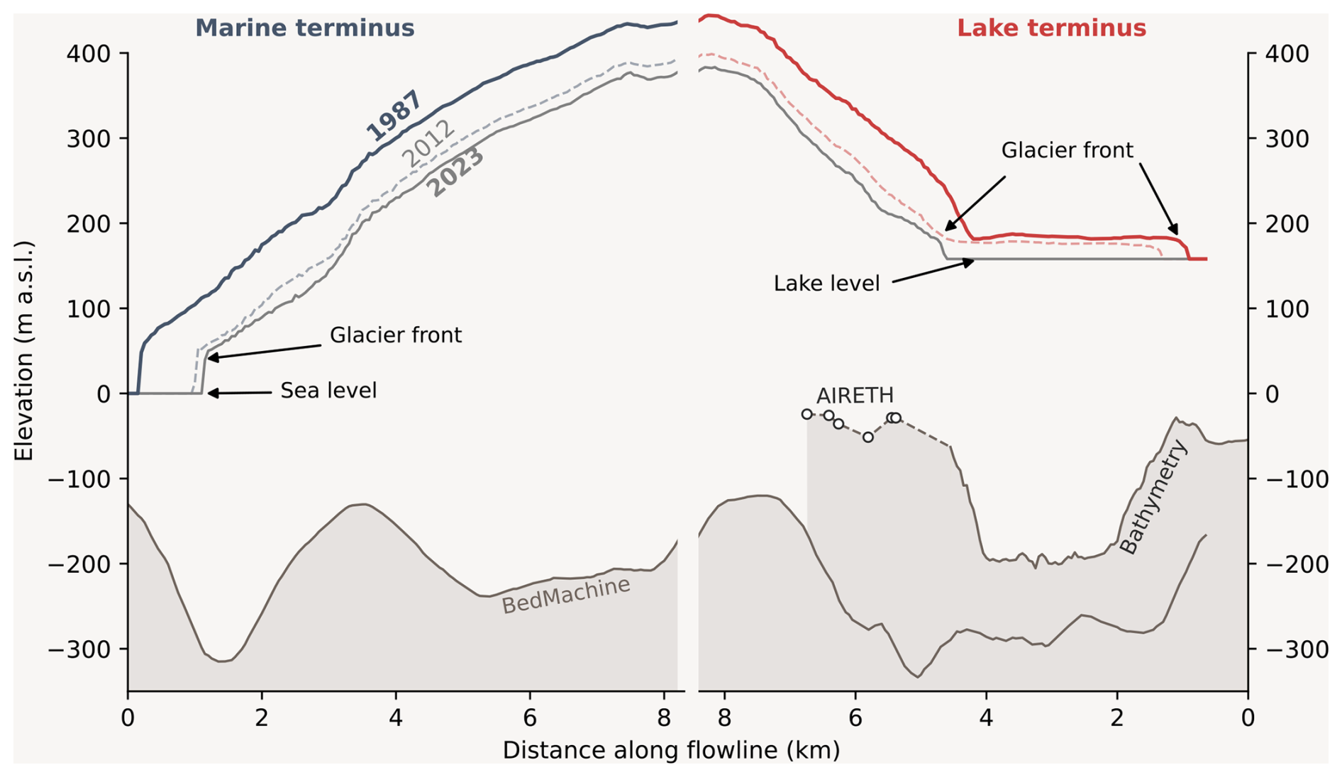
Figure 3 Surface elevation profiles for both glacier termini along the center lines indicated in Fig. 1. Glacier surface elevations are extracted from DEMs from 1987 (Korsgaard et al., 2016), 2012 and 2023 (Porter et al., 2022). The bedrock elevation from BedMachine v5 (smoothed) (Morlighem et al., 2022), AIRETH (Santin et al., 2026) and our bathymetry measurements are indicated by the shading.

By comparing thinning rates for both glaciers at the same elevation (> 200 m above sea level), we find that between 1987 and 2012, the thinning rates are similar, with 2.1 m yr⁻¹ (LT) and 2.0 m yr⁻¹ (MT). However, between 2012 and 2023, the thinning rate of the lake-terminating glacier exceeded that of the marine-terminating glacier by 0.4 m yr⁻¹, with rates of 1.7 and 1.3 m yr⁻¹, respectively. Both glaciers clearly show lower thinning rates after 2012.

4.2 Bathymetry and floatation

The bathymetric survey of Lake Motzfeldt reveals an exceptionally deep lake with a maximum lake depth of 368 m (Fig. 4a, red dot) and an average of 131 m. The lake is generally shallower south of the lake bend and gradually deepens toward the north. The lake morphology is characterised by steep side walls and a flat, deep middle part. At the position where the glacier was stagnant until 2012, a clearly visible ridge extends from the western lake shore to the middle of the lake (Fig. 4a). However, the composition of this ridge is unknown.

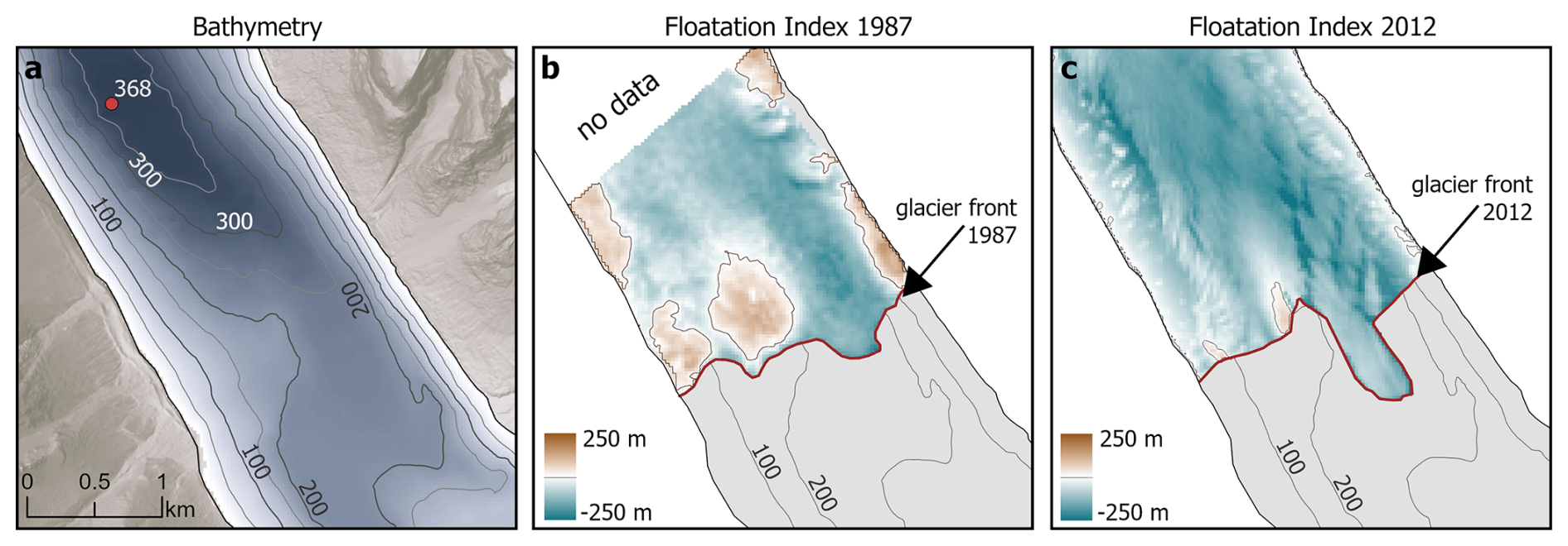
Figure 4 The bathymetry and floatation index at the LT glacier front. Panel (a) shows the results from the bathymetric survey of Lake Motzfeldt. The red dot marks the deepest point in the lake. Panel (b) and (c) show the floatation index at the glacier front in 1987 and 2012. Positive values indicate grounded areas. Negative values indicate floatation.

The floatation index shows that in 1987, extended parts of the glacier front were grounded on and upstream of the ridge, as well as on both lateral margins (Fig. 4b). On the ridge, the floatation index reaches values of up to 200 m, which means that the theoretical ice thickness, assuming floatation, exceeds the lake depth at that position by 200 m. Due to substantial thinning (see the previous section), most of the pixels classified as grounded in 1987 are classified as floating in 2012. The grounded area on the ridge was largely diminished with a maximum floatation index value of 80 in 2012. The DEM from 2012 shows that, at that time, the lateral margins of the glacier had crumbled apart, leading to the loss of grounded areas on the sides.

4.3 Lake temperature and lake level

The three CTD measurements show a cold lake with a depth-averaged temperature of about 0.65, 0.68 and 0.71 °C for CTD 1, 2 and 3 respectively (Fig. A2 in the Appendix). All CTD casts are coldest at the top and gradually become warmer toward the bottom. The coldest temperatures are found closest to the glacier front (CTD 1), and the warmest are farthest away (CTD 3). CTD 1 and 2 remain below 0.75 °C at all depths, while CTD 3 shows slightly warmer water at the bottom, with a maximum temperature of 0.86 °C. The time series of the temperature sensor that was placed from 2024 to 2025, shows that temperatures decreased from about 0.7 °C at deployment in August to 0.2 °C in November (Fig. A1). Between November and mid May, the lake water stays below 0.2 °C, with very little daily variation. Following that, temperatures rise again to a maximum of 0.8 °C in the end of July before starting to decrease again in September. The lake level, inferred from the sensor depth, remains approximately constant between the beginning of October and the beginning of July. In July, the lake level rises by 1.6 m compared to the winter low. In August and September, the lake level is generally high (1 m above winter low); however, it shortly lowers by 0.6 m at the end of August.

4.4 Dynamics at the lake terminus

We tracked changes in glacier front position with high temporal resolution between 2014 and 2024 and found a characteristic ice-shelf calving style at the lake-terminating glacier (Fig. 5). Following the disintegration of the ice tongue in 2012–2013, the LT glacier front has experienced prolonged phases of gradual front advance, interrupted by abrupt, large calving events. In some years, such as 2020, the advance phase persisted through the summer, with the glacier front advancing approximately 500 m over the entire year without any noticeable calving events. As shown in Fig. 2, the glacier advances primarily in the centre of the lake, with no lateral contact with the lake shore.

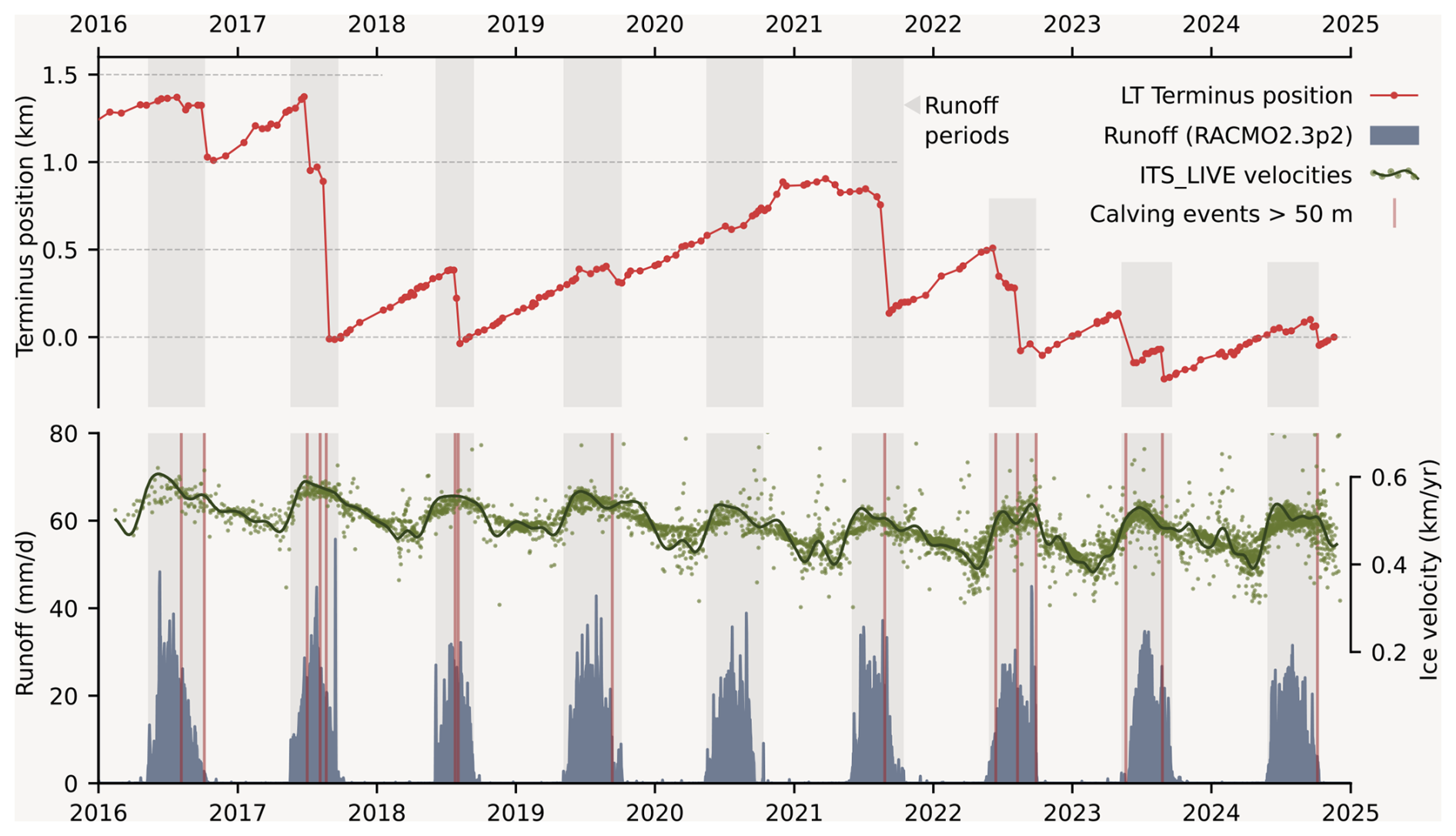
Figure 5 Dynamics at the lake terminus. The upper part of the figure shows the terminus position relative to the last observation. The lower part of the figure shows ice flow velocities at the glacier front from ITS_LIVE and TICOI (Gardner et al., 2025; Charrier et al., 2025). Daily runoff from RACMO2.3p2 (Noël et al., 2018) is shown with blue bars. Calving events, extracted from the front positions, are marked with red vertical lines in the lower part of the figure.

Between 2014 and 2024, we identified 15 major calving events, each resulting in a front retreat exceeding 50 m (Fig. 5). The largest single-event retreat measured 923 m, while the most substantial cumulative retreat measured about 1.4 km in the summer of 2017 during three consecutive events. From satellite images, we observed that these events produced large tabular icebergs that do not capsize. All calving events coincided with the runoff season and occurred during lake ice-free conditions on Lake Motzfeldt (Figs. 5, 6).

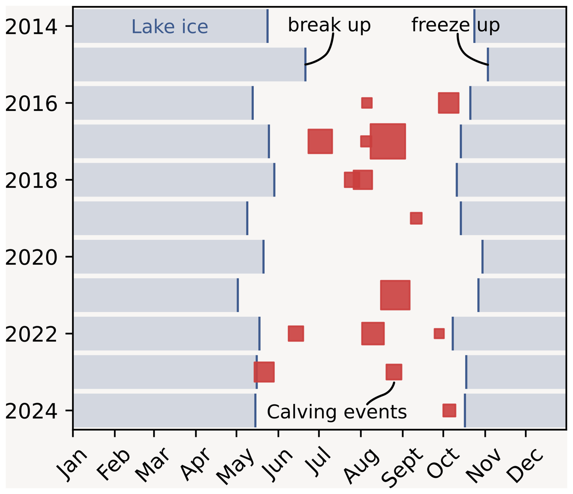
Figure 6 Duration of full lake ice cover and the timing of calving events at the lake terminus. The size of the squares depict the relative magnitude of events.

The duration of the full lake ice cover in Lake Motzfeldt averaged 212 d, ranging from 187 d in 2015 to 230 d in 2021 (Fig. 6). Lake ice cover generally developed in October, with one exception in 2015 where it developed in early November. The earliest onset of the full ice cover was observed on 8 October 2022. Lake ice break up usually occurs in May or June, the earliest recorded on 2 May 2021 and the latest on 21 June 2015.

In the observed period 2016–2024, the ice flow velocities at the lake terminus ranged between 380 and 610 m yr⁻¹, with a gradual decline in the average annual velocity from ∼ 544 m yr⁻¹ in 2016 to ∼ 472 m yr⁻¹ in 2024. A clear seasonal signal can be identified with a 15 % increase from winter (DJF) to summer (JJA) velocities. Ice flow velocities usually increase with the beginning of the runoff season and drop again at the end of the runoff season. In some cases, calving events coincide with small flow velocity increases (Fig. 5).

4.5 Dynamics at the marine terminus

Between 2014 and 2024, the marine-terminating glacier showed a distinct seasonal cycle, with front advance occurring on average between October and May and retreat from June through September (Figs. 7 and 8). Notable exceptions are the years 2019, 2020 and 2021, where retreat already started in February, April, and March, respectively. The average magnitude of front position change between winter and summer positions is 280 m. The largest differences occur in the years 2014–2016 with 350, 400 and 410 m difference between minimum and maximum positions.

Ice flow velocities at the glacier front ranged between 1.4 and 2.1 km yr⁻¹, with the lowest annual average velocities in 2024 (1.5 km yr⁻¹) and the highest during 2019–2021 (∼ 1.9 km yr⁻¹) (Fig. 7). During these peak years, velocities continued to accelerate even after the runoff season, reaching a maximum in December. As a result, the highest monthly velocities over the full period were on average during October through December. However, no clear seasonal signal can be identified.

Eight kilometres upstream, the ice flow velocities are notably lower, ranging from 0.7 to 0.9 km yr⁻¹. Similarly to the terminus, the highest annual velocities occurred in 2019–2022 and the lowest in 2024. Although velocities are on average highest in May, June, and July, seasonal variability is low, less than 4 %. In the upstream velocities, we see a strong acceleration each year coinciding with the beginning of the runoff period.

To assess potential drivers of terminus position variation, we compared monthly retreat rates with air temperature and runoff. We found a positive correlation of front position and runoff (r=0.6), and air temperature (r=0.5). As shown in Fig. 8, the runoff period aligns closely with the retreat period.

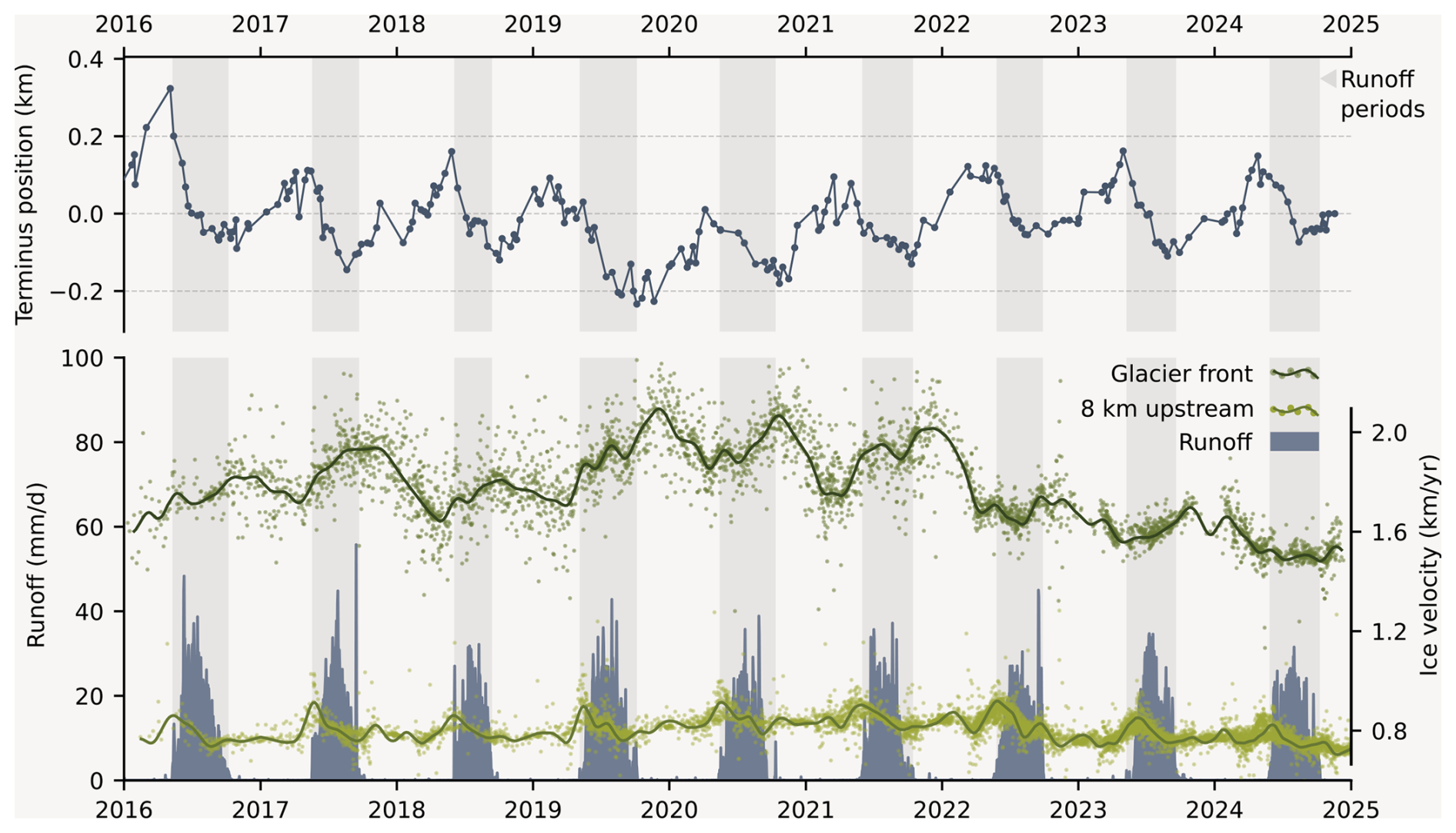
Figure 7 Dynamics at the marine terminus. The upper part of the figure shows the seasonal cycle of the glacier front positions relative to the last observation. The lower part shows ice flow velocities at the glacier front and 8 km upstream from ITS_LIVE and TICOI (Gardner et al., 2025; Charrier et al., 2025). The blue bars show daily runoff from RACMO2.3p2 (Noël et al., 2018). Note that the scales are different from those in Fig. 5.

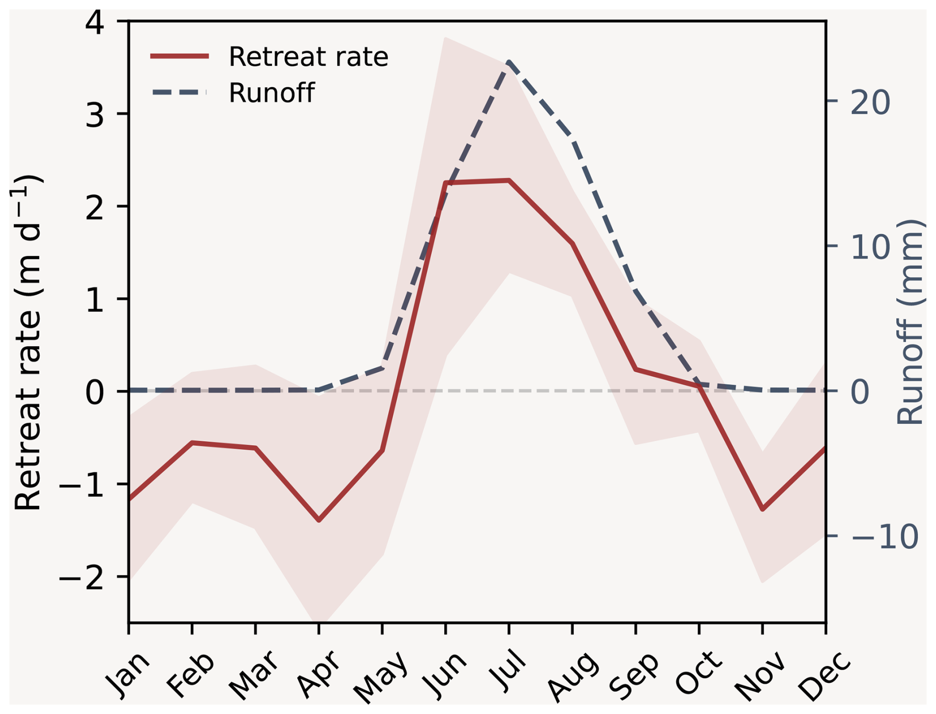
Figure 8 The average monthly retreat rate of the marine terminus of Qooqqup Sermia between 2014 and 2024 (red line with confidence interval as shading) and the average daily runoff per month (blue stippled line).

5 Discussion

In this section, we first discuss the historical evolution and the dynamics of the lake- and marine-terminating glacier before highlighting key differences between the two environments in a broader sense.

5.1 The floating ice tongue of the lake-terminating glacier

The flat morphology of the glacier surface, the production of large tabular icebergs, as well as the buoyancy compensated thinning rates of LT suggest that prior to 2012, a floating ice tongue was present at the lake terminus (Figs. 2 and 3). Although we are unaware of other descriptions of floating ice tongues in Greenlandic lakes, they are a common phenomenon in other regions like Patagonia (Warren et al., 2001), Alaska (Boyce et al., 2007; Trüssel et al., 2013), and Iceland (Benn et al., 2007). In Greenland, fully floating ice tongues are found at marine-terminating glaciers, but only in the very north (Hill et al., 2018; Millan et al., 2023; Wekerle et al., 2024) following the disintegration of several ice tongues further south (Millan et al., 2023; Mouginot et al., 2015; Johnson et al., 2004).

We believe that the formation and sustained presence (at least 1987–2012) of the ice tongue in Lake Motzfeldt in the very south of Greenland was possible for two main reasons. First, lake Motzfeldt is exceptionally deep and therefore provides the necessary geometry. Second, subaqueous melt rates in Lake Motzfeldt are low, therefore limiting thinning rates and promoting stability. This falls in line with Truffer and Motyka (2016) who suggest that floating ice tongues in lakes can occur in more temperate regions further south compared to marine-terminating glaciers due to colder water temperatures and the lack of salinity-driven circulation, which strongly limit subaqueous melt as well as calving as a result of undercutting of the glacier front. And indeed, our CTD and temperature measurements in Lake Motzfeldt show a very cold lake, with a depth averaged temperature at the glacier front of < 0.7 °C in August 2025. The lake can sustain such a cold temperature throughout the year due to meltwater input and the immense amount of icebergs present. Any additional energy input through solar radiation or heat advection is likely transferred into the icebergs, efficiently cooling the lake.

Nonetheless, in 2012 and 2013, several large calving events led to the disintegration and massive loss of more than 3 km of the glacier terminus. Our bathymetry data and the historical DEMs indicate that the disintegration of the floating ice tongue was due to the separation from a pinning point at the glacier front. These pinning points exert important backstress on the glacier, and their loss is known to have destabilising effects (Goldberg et al., 2009; Favier et al., 2012). In 1987, the glacier was well grounded at the pinning point. However, gradual thinning led to the almost complete separation from the the pinning point by 2012 (Figs. 3 and 4). Since the disintegration of the floating ice tongue, the glacier has changed to a mode of long advance phases followed by abrupt, large calving events. These calving events still produce large tabular icebergs, which indicates that a floating tongue develops each time during the advance phase, again pointing to low subaqueous melt rates.

5.2 Dynamics at the lake terminus

We observe a distinct calving pattern at the lake terminus that can be described as follows: The glacier experiences long advances phases that can persist throughout the melt seasons and can last longer than a full year. These advance phases are interrupted by the calving of large tabular icebergs (most larger than 200 m). Some calving events follow the formation of clearly visible rifts, while others don't show clear rift formation. Almost all icebergs detach from the glacier front and drift away without capsizing. This calving style is typical for fully floating ice tongues in Greenland (Bézu and Bartholomaus, 2024) and resembles that of large fully floating ice tongues in North Greenland, like Peterman (e.g. Johannessen et al., 2013) and Ryder Glacier (e.g. Holmes et al., 2021).

Remarkably, all documented calving events occur between mid May and mid October, coinciding with the runoff period. This could indicate that also buoyant forces play a role in triggering calving events, as it was observed at several other lake-terminating glaciers (Howarth and Price, 1969; Holdsworth, 1973; Warren et al., 2001). During the runoff period, buoyant forces are increased through thinning of the glacier from the surface as well as through a rise in lake level due to increased meltwater input (Fig. A1). Furthermore, we observe that all calving events occur outside of the lake ice covered period. Although lake ice could provide some backstress to the glacier, it is unclear as to what magnitude and what effect it would have on calving. However, we believe that lake ice possibly functions as a binder, preventing icebergs from drifting away, helping to keep the glacier front together during winter.

Ice flow velocities are generally slower at LT compared to the center of MT, which already is apparent at the beginning of LT where it branches off from MT. These velocity differences may stem from the bedrock geometry. The overall elevation drop is likely higher for MT than for LT, as the latter terminates in Lake Motzfeldt about 160 m above sea level, whereas MT extends to sea level. Bedrock data from BedMachine (BM) version 5 (Morlighem et al., 2022) indicates a small bump at the start of LT which could slow down the flow from MT into the valley of LT (Fig. 3). Unfortunately, bedrock measurements in South Greenland and on Qooqqup Sermia in particular are notoriously difficult to obtain, and BM relies on poorly constrained indirect estimates (Morlighem et al., 2017; Santin et al., 2026). However, recent measurements by Santin et al. (2026) with AIRETH, a redesigned helicopter-borne ground-penetrating radar, show that the bedrock elevation at LT is even higher than reported in BM and that the bedrock slope toward the glacier front is likely less steep (Fig. 3). Measurements with the same system along the marine terminus of Qooqqup Sermia could not recover reliable bed returns, indicating a greater ice thickness. As a result, the bedrock geometry beneath LT is now better constrained, while BM remains unreliable at MT, making a comparison of bed geometry between the two termini difficult. In addition to the bedrock geometry, it appears as LT is fed by the slower lateral ice from the margins of MT rather than by its fast central trunk.

Despite their large magnitude, calving events do not appear to have an effect on the glaciers flow velocities, as flow velocities only seem to follow a pattern of a swift increase at the onset of the runoff season and a progressive decrease at the end of the season (Fig. 5).

5.3 Historical evolution of the marine terminus

The historical evolution, the seasonal front position, as well as the ice flow velocity largely resemble those of other marine-terminating glaciers in Greenland, with differences discussed below. Dissimilar is the net advance during the pre-satellite era (here 1953–1992) of about 640 m. Notably, Warren and Glasser (1992) describe a retreat of the glacier front between 1942, 1953 and 1981, indicating that the advance must have occurred only between 1981 and 1992, surpassing the initial retreat. Although mean annual air temperatures were considerably lower than average for a few years in the early 1980s, it is difficult to pinpoint the cause of the advance. For the neighbouring Eqalorutsit Kangilliit Sermiat, Weidick (2009) also describes an anomalous advance (during a more extended period 1942–2000), noting a complicated precipitation pattern with large spatial variations over a small area as a possible cause.

After reaching its most advanced position in 1994 the glacier recedes about 1.3 km until 2004, where it remains stable until today. Although the cause of the retreat of other marine-terminating glaciers in Greenland during that period is often induced by warming ocean temperatures (Wood et al., 2021), we lack oceanographic data in the inner fjord to confirm this at Qooqqup Sermia. Furthermore, it appears that the position before 2004 was an overextension of the glacier to an unstable position without any visible pinning points. An indication of this is that the glacier front did not remain at a specific position before 2004, but rather changed every year.

5.4 Dynamics at the marine terminus

Since 2004, the glacier remained at approximately the same position with seasonal ice-front advance during winter (October–May) and retreat during summer (June–September). The position around which the glacier front oscillates is characterised by a visible narrowing of the fjord through a bedrock protrusion on either side. Seasonal advance and retreat of glacier fronts are common phenomena (Schild and Hamilton, 2013; Moon et al., 2015; Black and Joughin, 2023), observed at more than 80 % of marine-terminating glaciers in Greenland (Greene et al., 2024). This seasonality of glacier front positions has been suggested to be mainly driven by meltwater runoff (Black and Joughin, 2023; Fried et al., 2018) and the presence or absence of an ice mélange (Joughin et al., 2008; Todd and Christoffersen, 2014; Cassotto et al., 2015; Kneib-Walter et al., 2021; Wehrlé et al., 2023), both of which affect the calving rate. In agreement with these findings, we observe that the majority of Qooqqup Sermia’s frontal retreat takes place during the runoff season, whereas most of its advance occurs outside of the runoff season (Figs. 7 and 8), indicating that the ice-front position is influenced by submarine melting due to meltwater runoff. This is supported by observations during both field campaigns and on satellite images, where we observed meltwater plumes for extended periods during the melt season (see Fig. A3). These plumes, formed by runoff entering the fjord subglacially, enhance submarine melting and can trigger calving by undercutting the ice-front (Rignot et al., 2015; Fried et al., 2015; Slater et al., 2017; Hewitt, 2020). Figure A3b also shows strong undercutting of the glacier front at the location of the plume. The calving that we observe at MT can be classified as serac collapse type (Bézu and Bartholomaus, 2024) with frequent calving of small icebergs.

However, in some years, the coupling of ice-front position and runoff is slightly less evident. In the years 2019–2021 the front position starts to retreat before the beginning of the melt season. Similar observations at other glaciers showed that this can be caused by an early clearing of the ice mélange and the accompanied reduction of resistive stresses at the glacier front (Cassotto et al., 2015; Bevan et al., 2019; Wehrlé et al., 2023). However, we have no time series documenting the presence of an ice mélange at Qooqqup Sermia to confirm this. Therefore, we conclude that the seasonality of glacier front positions is influenced by subglacial runoff, however, with other processes likely also playing role.

As is typical for calving glaciers, Qooqqup Sermia's flow velocity also increases towards the terminus, thereby more than doubling its speed from 8 km upstream to the glacier front. The upstream ice-flow velocities remain relatively constant throughout the observation period, with a notable spike at the beginning of the runoff season each year. This short-term increase in flow velocities is also observed in other regions of Greenland (van de Wal et al., 2008) and can be linked to the efficiency of subglacial drainage when meltwater or rainwater enters the system (Bartholomaus et al., 2008; Schoof, 2010). At the glacier front, ice flow velocities begin to accelerate in late spring and continue to accelerate even after peak runoff is reached, indicating a decoupling from runoff after initial acceleration (Fig. 7). This is observed for many glaciers in Greenland as shown by large scale (Moon et al., 2014; Vijay et al., 2019) and case specific studies (e.g. Zhang et al., 2025). Moon et al. (2014) show that for this category of glaciers (called “type-1”), ice flow velocity is closely coupled to changes in ice-front position. Also, at Qooqqup Sermia, we observe that the highest flow velocities coincide with the most retreated glacier front positions. This can be explained by reduced resistive stresses when the ice front retreats behind the pinning point (Bevan et al., 2012; Howat et al., 2008).

5.5 Key differences between the lake and marine terminus and potential causes

In previous sections, we illustrated that the lake- and marine-terminating glacier exhibit contrasting dynamics, despite being subject to the same climatic conditions. The key differences can be summarised as the following: We observe the marine terminus to be a fast flowing, grounded glacier with frequent small-size calving events, mainly in the form of serac failure type. The lake-terminating glacier, on the other hand, has a floating extension and experiences rare, but very large calving events, producing large tabular icebergs. Furthermore, MT shows a clear seasonality with glacier front retreat in summer and advance in winter as well as a coupling of ice flow velocities to the glacier front position. In contrast, LT does not have seasonal ice front fluctuations, and ice flow velocities do not seem to be coupled to the front position.

Differences in bedrock geometry and ice thickness certainly partly determine the dynamics at the two termini. However, in addition, we identified the following physical differences between the two environments, which potentially influence the morphology and dynamics at the glacier termini. The following considerations apply to this study and, in general, to the comparison of marine- and lake-terminating glaciers.

1. Freezing point depression: In the marine environment, the freezing point of ocean water is lowered due to the salt content. With a salinity of 32 PSU the freezing point drops to about −1.8 °C. A lower freezing point increases the thermal driving (or thermal excess), consequently increasing submarine melt rates. Even in a cold ocean environment this freezing point depression leads to higher melt rates compared to a freshwater environment. For example, assuming an ocean temperature of 0.6 °C (average temperature of the top 100 m measured by Hansen et al. (2025) in Tunulliarfik Fjord, close to Qooroq Fjord) and a lake temperature of 0.7 °C (measured in lake Motzfeldt) results in a thermal driving that is 3 to 4 times higher in the ocean compared to the lake (2.4 °C vs. 0.7 °C above the freezing point).

2. No subglacial plume formation: The formation of subglacial plumes can significantly enhance submarine melt rates (Jenkins, 2011), promote undercutting, and consequently calving (Slater et al., 2017). However, lakes generally consist of freshwater and therefore lack vertical circulation at the ice front, driven by the density differences of fresh and salt water (Truffer and Motyka, 2016). Consequently, we observe the formation of subglacial plumes at MT but not at LT, arguably leading to even higher melt rates at MT compared to LT. Furthermore, this implies that additional runoff at MT would enhance melt rates by generating stronger plumes, whereas in the lake, additional runoff would not affect melt rates and could even cause the lake to cool. This could possibly explain why seasonality in front positions is observed at MT but not at LT.

3. Heat transport: A lake is a semi-closed system where no transport of large quantities of warm water masses toward the glacier front from distant sources takes place. The energy input to the lake is limited to long and short wave radiation, heat exchange with the atmosphere, and advected heat (e.g., rainwater, streams, and groundwater) (Wetzel and Likens, 2000). In the fjord, on the other hand, water masses can be transported to and from the glacier front through ocean circulation and exchange with more distant water masses. Even in fjords with a prominent sill, exchange with shelf water is not completely blocked, and cold water can be transported away and exchanged with warmer waters (e.g. Mortensen et al., 2018).

The differences outlined above clearly demonstrate that subaqueous melt rates must be higher at MT than at LT, even with cold ocean conditions. The presence of a meltwater plume, the undercutting of the ice front, and the correlation between surface runoff and glacier front position all suggest that submarine melting affects the dynamics of the marine-terminating glacier. At LT on the other hand, low melt rates create favourable conditions for a floating extension of the glacier through limited thinning and calving rates. This comparison indicates that the difference in subaqueous melt rate contributes to the contrasting dynamics that we observe.

6 Conclusions

In this study, we compared two adjacent glacier termini of the Qooquup Sermia glacier system, one of which is lake-terminating and the other is marine-terminating. From our analysis, we draw the following conclusions:

• The marine terminus of the Qooqqup Sermia system is fast flowing, grounded, characterised by frequent small calving events, and experiences seasonal front advance and retreat. Ice flow velocities are coupled to the ice front position.

• The lake terminus, on the other hand, has a floating extension and experiences rare but large calving events, producing tabular icebergs. The lake terminus does not have seasonal ice front fluctuations and ice flow velocities do not seem to be coupled to the front position.

• We infer extremely low subaqueous melt rates at the lake terminus as one of the main differences between the two environments. These low melt rates create favourable conditions for a floating ice tongue in the lake by limiting thinning and calving rates.

• The massive retreat of more than 3 km of the lake terminus in one year highlights the possibility of rapid mass loss at lake-terminating glaciers in Greenland, stressing their importance for the future evolution of the Greenland ice sheet. The retreat was likely connected to the separation from a pinning point.

Appendix A

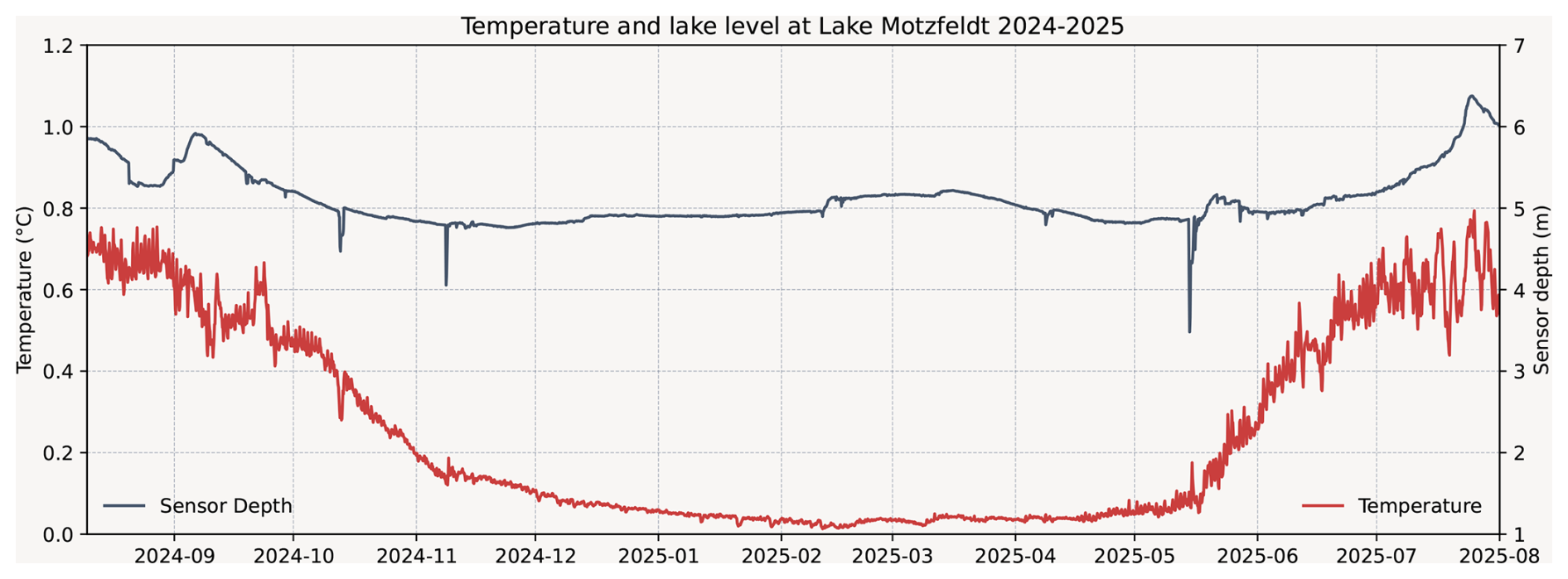
Figure A1 Temperature and sensor depth (meter water pressure) time series of the RBR sensor in Lake Motzfeldt. The location of the sensor is shown in Fig. 1. The sharp spikes in the depth data (pressure decrease) are due to the rope to which the sensor was attached, being moved, likely by icebergs or drifting lake ice. A pressure increase during winter (e.g mid February) can be linked to snow accumulating on the lake ice.

Figure A2 CTD measurements in Lake Motzfeldt. The locations are indicated in Fig. 1.

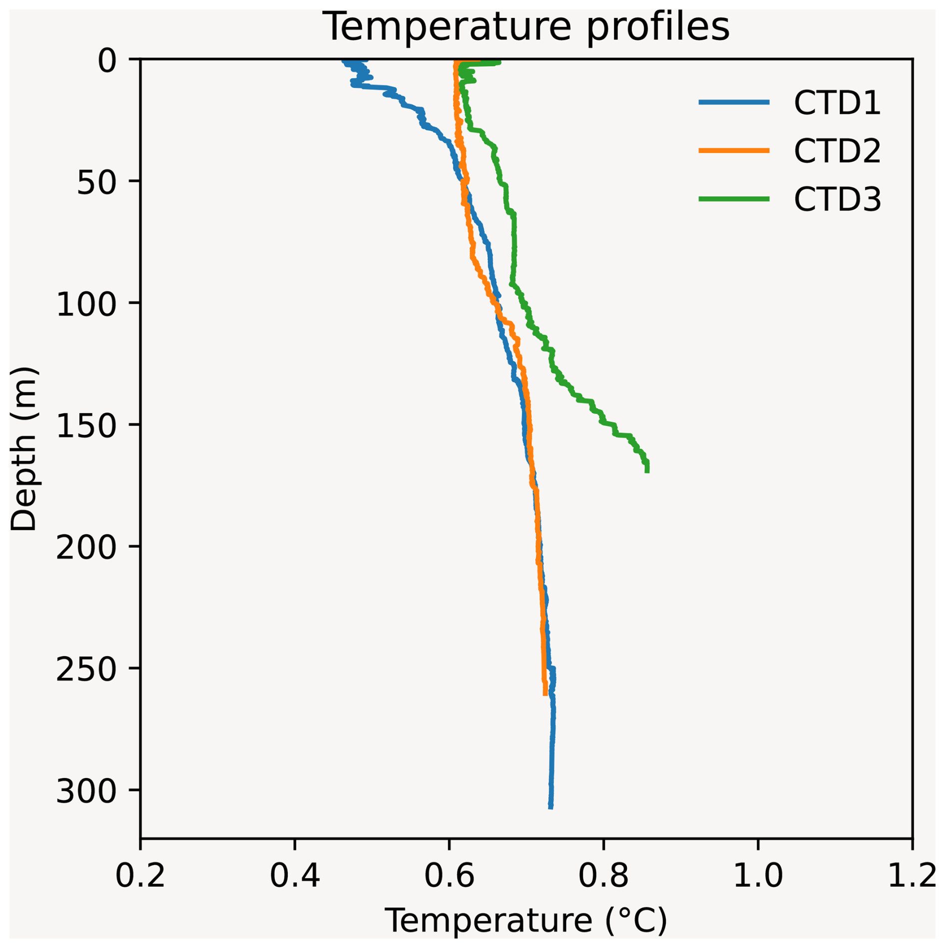
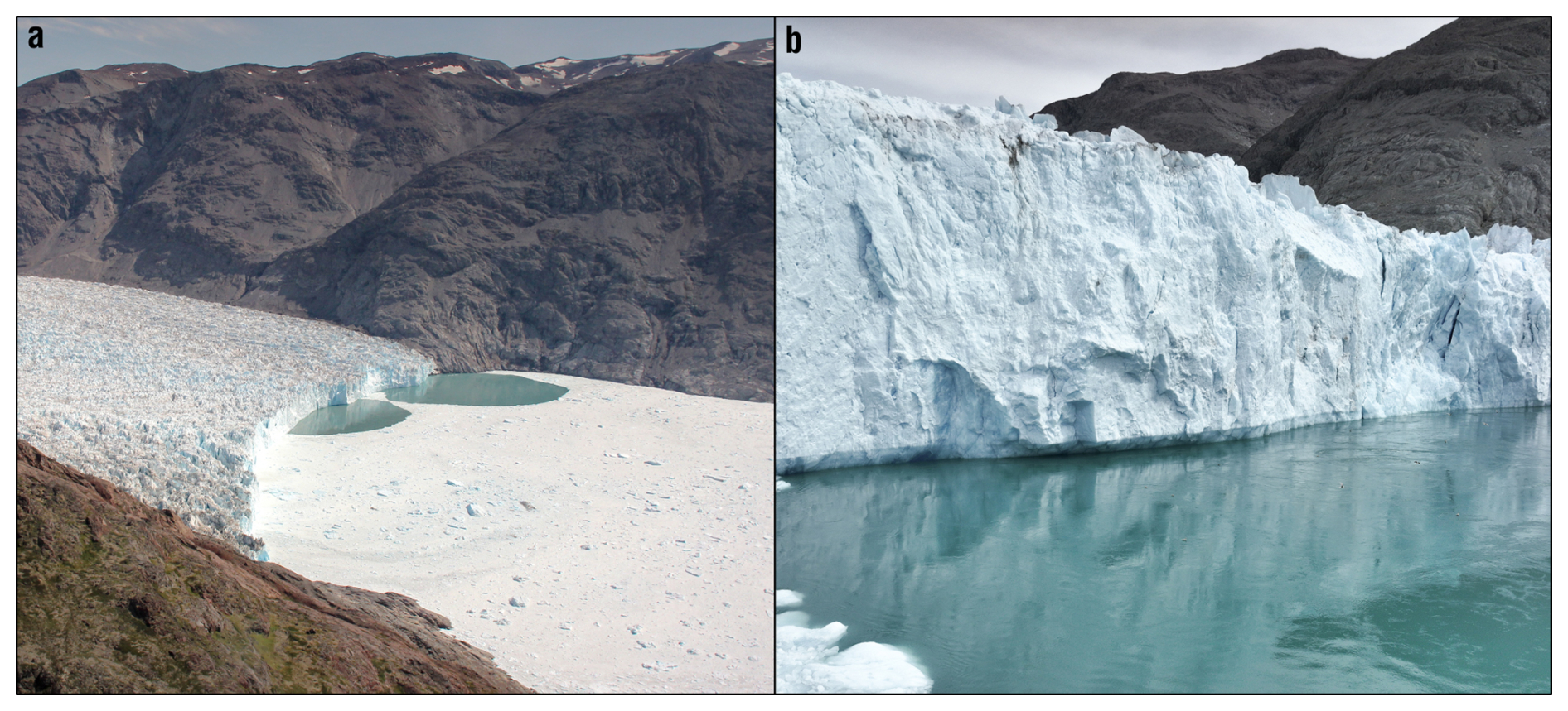
Figure A3 Melt water plume at the marine terminus of Qooqqup Sermia (a) two plumes observed at Qooqqup Sermia on 26 July 2025 (b) close up drone image showing the plume and undercutting at the glacier front.