30 m monthly glacier surface velocity mapping in the Kangri Karpo region (2015–2024) using multi-source remote sensing data fusion

To improve the accuracy and timeliness of glacier surface-velocity retrieval in complex mountain terrain, we develop a high-spatial-resolution fusion method combining Landsat, Sentinel-1/2, and UAV (Unmanned Aerial Vehicle) data, and produce monthly velocity products for the Kangri Karpo region for 2015–2024. Compared with existing large-area public datasets, the products offer markedly higher spatial resolution and better detection of small mountain glaciers; relative to single-sensor inputs prior to fusion, the valid-pixel ratio increases by ∼50 %, the average number of valid months per pixel over the decade rises by ∼50, and spatial smoothness improves – demonstrating the method's suitability for rugged terrain. Spatially, velocities follow the canonical “fast center, slow margins” pattern, with multi-year maxima >700 m yr⁻¹ and values in lower reaches and most tributaries generally <100 m yr⁻¹. Attribute analysis indicates significant correlations between velocity and area, slope, and aspect: larger glaciers flow faster overall; within individual glaciers, velocity responds more strongly to slope; and, with similar area and slope, south-facing glaciers are slightly faster than north-facing ones. Temporally, the intra-annual series shows clear seasonality, with peaks at the beginning and end of the melt season and sustained high speeds throughout. At the interannual scale, most pixelwise decadal trends lie within −36.5 to +36.5 m yr⁻¹ per decade (overall subdued change), and the median trend is slightly positive, indicating weak regional acceleration; ∼38.3 % of glaciers accelerate significantly, 25.5 % decelerate significantly, and 36.2 % show no significant trend (p≥0.05). By aspect, significant acceleration is concentrated on south- and west-facing glaciers, whereas significant deceleration occurs mainly on east- and north-facing glaciers. Month-resolved trends indicate acceleration primarily in April–May (∼54.7–73.0 m yr⁻¹ per decade), likely linked to enhanced meltwater input from an advanced melt season, and deceleration concentrated in July–August ($\le -\mathrm{54.7}$ m yr⁻¹ per decade), plausibly associated with intensified mass deficit.

1 Introduction

The cryosphere is an integral component of Earth's climate system, encompassing ice sheets, glaciers, permafrost, seasonal snow, and sea ice, and it serves as a key indicator and regulator of global climate change (Slaymaker and Kelly, 2007). As a major subsystem of the cryosphere, glaciers are both principal reservoirs of global freshwater and highly sensitive to warming; their retreat and accelerated melt exert far-reaching impacts by altering the hydrological cycle, modulating atmospheric circulation, and driving sea-level rise (Huss and Hock, 2015; Zemp et al., 2019). Evidence shows that glacier mass loss is now among the leading contributors to global sea-level rise (Ren et al., 2011; Liu et al., 2021), and its evolution affects regional water security while playing a significant role in climate-system feedbacks (Fountain et al., 2012).

Within the global glacier system, mountain glaciers account for only a small share of total ice storage but respond more sensitively to climatic perturbations (Zhang et al., 2015; Chen et al., 2019). Their meltwater directly shapes the spatiotemporal distribution of downstream runoff and underpins ecosystem stability (Slemmons et al., 2013; Zhang et al., 2020). In mid- to low-latitude, high-elevation regions such as the Qinghai–Tibet Plateau, glacier change not only governs headwater hydrology (Nan et al., 2025; Yao et al., 2023) but also has far-reaching implications for agriculture, ecosystems, and disaster-risk management (Zhang et al., 2007, 2020). Consequently, sustained, fine-resolution monitoring of mountain-glacier change is foundational for regional water-resource assessments and studies of climate responses (Zongxing et al., 2016).

Among the available indicators, glacier surface velocity is the central metric linking ice dynamics and mass balance. It captures the mechanical regulation of ice flow and associated energy-mass transfers, offering direct utility for diagnosing climate-forced dynamic responses, assessing downstream hydrologic risk, and characterizing glacier–climate coupling (Luckman et al., 2003; Huang and Li, 2011). Traditional in-situ techniques (e.g., theodolite, total station, GPS stake methods) yield high-accuracy point measurements but are constrained by high-elevation conditions, limited accessibility, and labor costs, impeding sustained, basin- to region-scale monitoring (Yan et al., 2015). By contrast, remote sensing – non-contact, synoptic, and repeatable – has become the primary approach for velocity monitoring (Luckman et al., 2007; Fan et al., 2019; Fu et al., 2022). Recent advances in multi-source data fusion and state-of-the-art algorithms have markedly improved the spatiotemporal resolution of velocity retrievals, strengthening our capacity to resolve dynamical evolution and its climatic drivers (Wang et al., 2019; Mohanty et al., 2025).

Recent studies have further advanced the integration and regularization of multi-sensor glacier-velocity observations. For example, Derkacheva et al. (2020) explored statistical and regression-based approaches for reducing and combining ice-velocity information derived from Landsat-8, Sentinel-1, and Sentinel-2. Greene et al. (2020) developed an approach for detecting seasonal ice dynamics from satellite image pairs, highlighting the importance of resolving sub-annual velocity variability. More recently, Charrier et al. (2025) proposed the TICOI framework to generate temporally regularized glacier-velocity time series from heterogeneous and overlapping multi-sensor observations. These studies demonstrate the growing importance of multi-source integration and time-series regularization for improving the continuity and interpretability of glacier surface velocity products.

Located at the eastern terminus of the Nyainqêntanglha Range in the southeastern Qinghai–Tibet Plateau, the Kangri Karpo region is one of the Plateau's most humid, maritime-glacier clusters, strongly influenced by the Indian monsoon, with elevations ranging from ∼2400 to 6600 m (Wu et al., 2021). Glacier area and volume there have changed markedly over recent decades. In 2015, the total glacierized area was approximately 2048.50 ± 48.65 km² (Wu et al., 2021), whereas in the 1980s it reached 2728.00 ± 34.24 km² (Wu et al., 2018). This implies a reduction of about 679.51 ± 59.49 km² – roughly 24.9 % of the total area – over the past three-plus decades (Wu et al., 2018), underscoring the region's pronounced sensitivity to climate change.

At present, no dedicated glacier surface-velocity dataset exists for the Kangri Karpo region. Global products that cover the area include: (i) GoLIVE (Global Land Ice Velocity Extraction from Landsat 8), derived from Landsat OLI imagery using the Python Correlation (PyCorr) image cross-correlation workflow, spanning 1 May 2013 to 30 April 2017 with a 16 d temporal resolution and 300 m×300 m spatial resolution (Fahnestock et al., 2016; Lei et al., 2021); and (ii) ITS_LIVE (Inter-mission Time Series of Land Ice Velocity and Elevation), produced with autoRIFT (autonomous Repeat Image Feature Tracking) from Landsat 4/5/7/8 imagery under NASA's MEaSUREs program, covering glaciers larger than 5 km² from 12 November 1982 to 27 April 2019, with temporal resolution of 6–546 d and 240 m×240 m spatial resolution (Gardner et al., 2018). Both datasets are available from the National Snow and Ice Data Center. However, these products have notable limitations: (1) relatively coarse spatial resolution, which hampers characterization of fine-scale velocity heterogeneity; (2) discontinued updates, limiting near-real-time monitoring and long-term trend analyses for recent years; and (3) substantial data gaps (NoData), which reduce completeness and reliability and complicate analysis. In sum, high-spatial-resolution glacier surface-velocity products remain scarce for the Kangri Karpo region.

The Kangri Karpo region features rugged relief and persistent cloud cover, which pose substantial challenges for remotely sensing glacier surface velocity. Optical sensors offer high spatial resolution, but their applicability is strongly constrained by persistent cloud cover, seasonal snow, and illumination effects such as topographic shadowing, especially for small glaciers in steep valleys, thereby limiting temporal coverage and data usability (Scherler et al., 2008; Berthier et al., 2005). Radar sensors operate in all weather and penetrate clouds, yet mountainous terrain induces layover, shadowing, and geometric distortions, leading to spatial data gaps (Kääb et al., 2005; Zhou et al., 2014). Consequently, fusing optical and radar observations provides complementary strengths in spatiotemporal resolution, observational completeness, and robustness, markedly improving the continuity and accuracy of velocity monitoring (Fan et al., 2019; Mohanty et al., 2025; Ye et al., 2024; Maksymiuk et al., 2016). This multi-source integration has become a key research direction for complex mountain-glacier environments, including the southwestern Tibetan Plateau.

Motivated by these limitations, this study develops a multi-sensor glacier surface-velocity product for the Kangri Karpo region. We perform weighted fusion of velocities derived from Landsat OLI, Sentinel-1 GRD, and Sentinel-2 MSI imagery to generate a high-spatiotemporal-resolution dataset for 2015–2024. We then examine spatiotemporal variability at decadal and seasonal scales to characterize glacier dynamics across the region, providing new support for glacier-velocity research in southeastern Tibet.

2 Study area

Located at the eastern terminus of the Nyainqêntanglha Range on the southeastern Qinghai–Tibet Plateau, the Kangri Karpo region is a relatively wet sector of the Plateau (Wu et al., 2021). It spans 29°00^′–29°30^′ N and 96°20^′–97°10^′ E, with elevations from ∼2400 to 6600 m.

Climatically, the area lies within the monsoonal temperate glacier region and is strongly influenced by the Indian monsoon (Yang et al., 2008), with pronounced seasonal hydroclimatic variability and frequent cloud cover. Owing to recent warming, glacier area and volume have declined markedly over recent decades, with signs of accelerated ablation. Given the region's complex climatic setting, Kangri Karpo glaciers exhibit pronounced sensitivity to climate variability, and their dynamics closely track local atmospheric fluctuations (Wu et al., 2021).

Glaciers are widely distributed across the massif. According to RGI 7.0 (RGI Consortium, 2023), the region contains 218 glaciers (Fig. 1): 162 smaller than 1 km², 30 between 1 and 5 km², and 26 larger than 5 km². Among the largest, the Yanong and Xirinongpu glaciers have surface areas of approximately 165 and 94 km², respectively. According to the published surge-type glacier inventory for High Mountain Asia (Lv et al., 2022; Guillet et al., 2022), no glaciers within our study area are identified as surge-type glaciers. Accordingly, surge-type behaviour is not considered in the subsequent analysis.

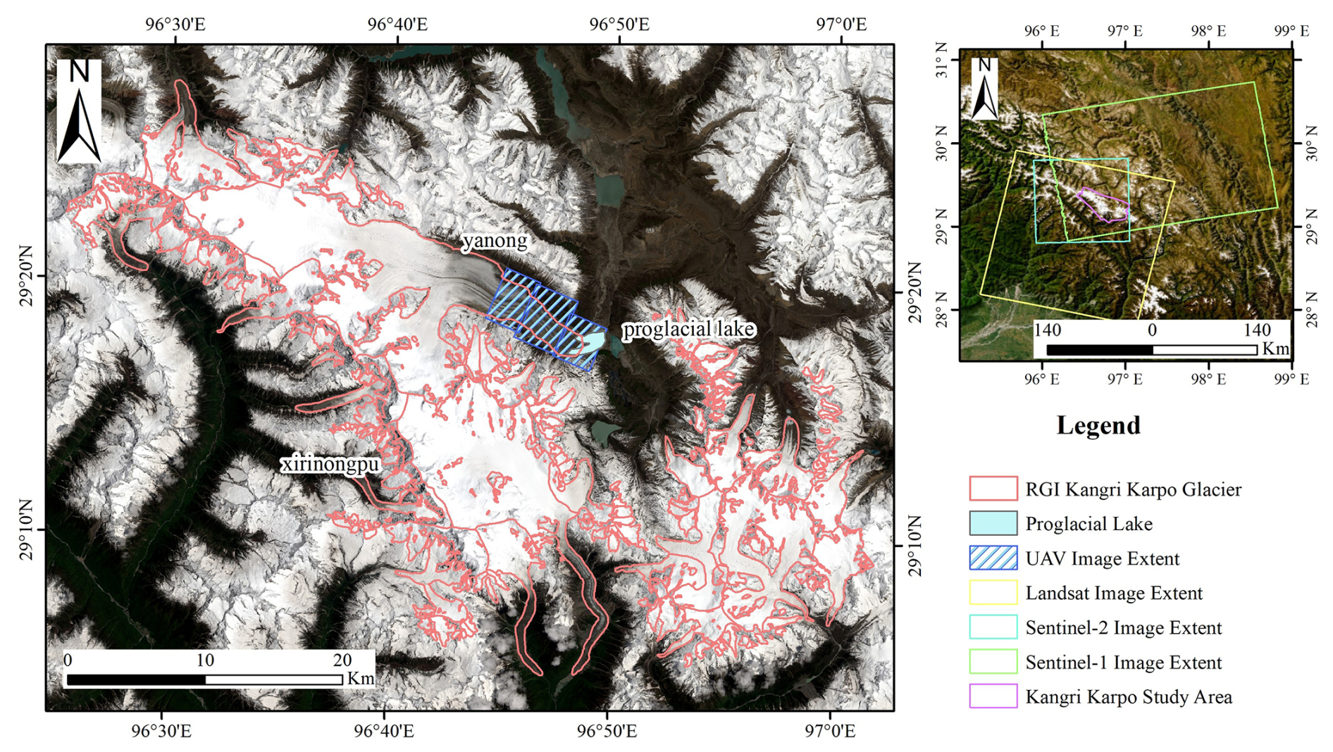
Figure 1 Study area of the Kangri Karpo region. Background: true colour image from Landsat 8/9 Collection 2 Level-1 (scene ID LC09_L1TP_134040_20230902_20230902_02_T1; acquired 2 September 2023), courtesy of the USGS (https://glovis.usgs.gov, last access: 11 September 2025). Inset (upper-right panel): Esri World Imagery (https://www.arcgis.com, last access: 11 September 2025) | Powered by Esri.

Beyond its climatic significance, Kangri Karpo is a key region for understanding glacier change across the Qinghai–Tibet Plateau. Continued retreat is likely to affect local ecosystems, water-resources management, and livelihoods. Long-term monitoring and analysis are therefore essential for anticipating future water-supply shifts and informing strategies to adapt to climate change.

3 Materials and methods

3.1 General workflow

To obtain a high spatiotemporal resolution glacier surface-velocity product for the Kangri Karpo region (monthly, 30 m), we designed a workflow centered on multi-sensor data fusion. The rationale is to exploit the complementarity of optical and radar observations: first retrieve displacements/velocities for each sensor stream using robust methods, then estimate fusion weights and repair gaps to produce a spatially consistent monthly field, followed by uncertainty quantification and spatiotemporal analyses.

Key steps are as follows: (1) Image pairing and preprocessing: Assemble monthly image pairs from Landsat-8/9 OLI and Sentinel-2 MSI (optical) and Sentinel-1 IW GRD (radar); perform geometric co-registration and basic corrections(e.g., applying orbit files to Sentinel-1 images). (2) Optical velocity retrieval: Apply frequency-domain phase correlation (COSI-Corr) for feature matching; derive east–west (E–W) and north–south (N–S) displacements and convert them to daily-mean speeds. (3) Radar velocity retrieval: Use intensity-based pixel-offset tracking on Sentinel-1 to estimate range/azimuth offsets in SAR image geometry, then apply terrain correction to geocode the results to map-projected ground geometry and convert them to velocity, providing stable coverage under cloudy conditions. (4) Temporal robustification and quality control: Remove mismatches using the signal-to-noise ratio (SNR) threshold and a robust time-series filtering method (described in detail later in Sect. 3.3) to improve cross-sensor consistency and reliability. (5) Constrained least-squares-based weighted fusion (CLS-based fusion): With co-temporal UAV-derived velocities as reference, estimate optimal weights for optical and radar fields and fuse them on a common grid, yielding a monthly product with fewer gaps and reduced noise. (6) Sentinel-1-guided gap filling: For residual voids, construct a spatially smoothed enhancement-coefficient field from the relationship between Sentinel-1 and the preliminary fused velocities, and use it to reconstruct missing pixels and improve spatiotemporal continuity. (7) Fusion evaluation and spatiotemporal analysis: Assess fusion performance using multiple diagnostics, quantify uncertainties, and analyze decadal and seasonal variability using the fused series.

The complete workflow is illustrated in Fig. 2.

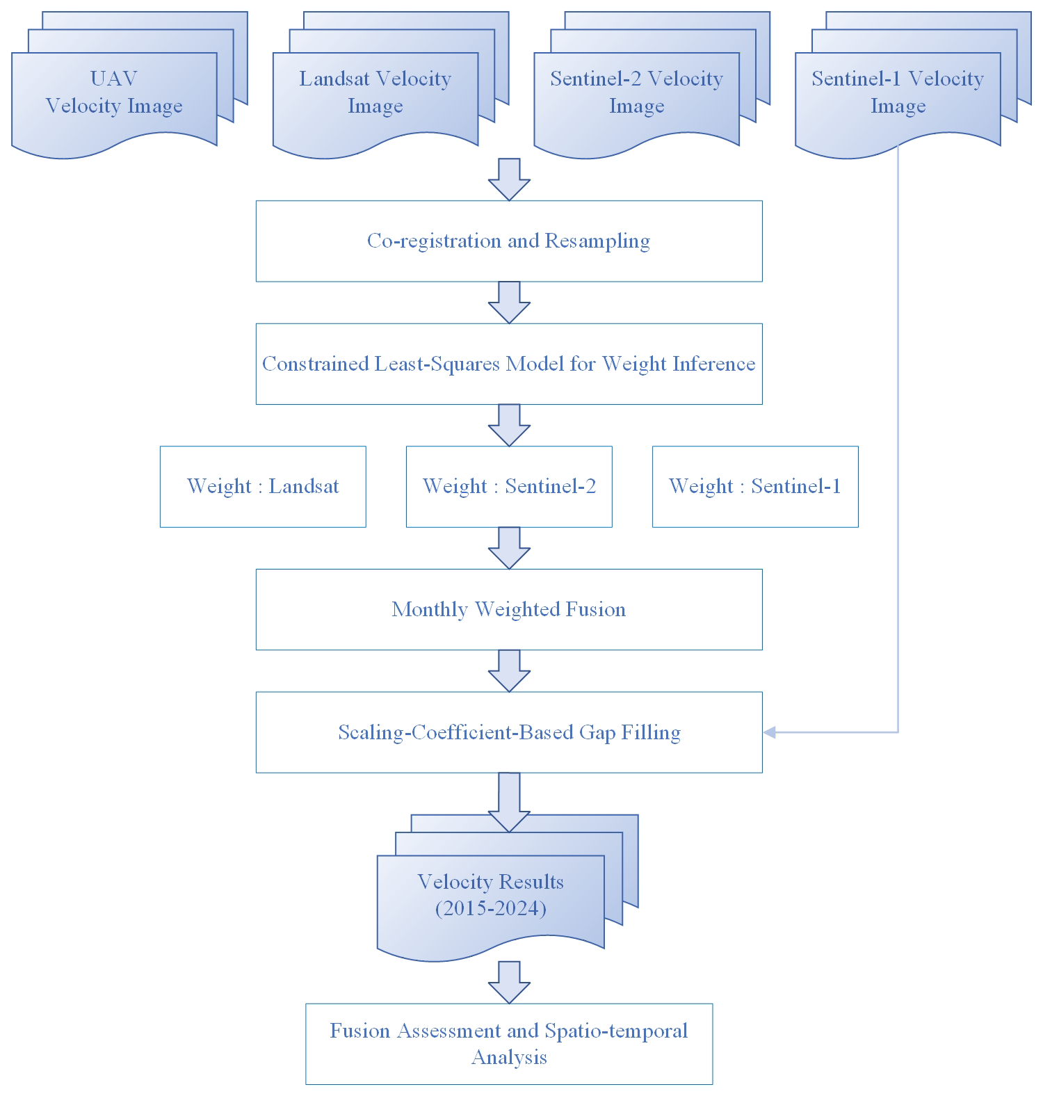
Figure 2 Workflow of this study. Input datasets and outputs are shown in gradient blue; processing and analysis steps are shown in white.

3.2 Imagery selection

For Landsat OLI imagery, we used Band 8 (panchromatic; 15 m). Scenes were downloaded from the USGS (http://glovis.usgs.gov, last access: 11 September 2025) as Collection-2 Level-1 products, which are system-corrected and directly suitable for analysis. To approximate a monthly product, we preferentially selected low-cloud scenes and paired acquisitions from the beginning and end of each month. Given the frequent cloud cover over high mountains, some months required extending the pairwise time interval to mitigate cloud contamination. The detailed information on the Landsat imagery used in this study is provided in Table S1 in the Supplement.

For Sentinel-1, we used Interferometric Wide (IW) mode, Ground Range Detected (GRD) scenes. To target a monthly cadence, we paired images near month start and end; because Sentinel-1A has a 12 d revisit, monthly coverage is not exact, and most pairs have temporal baselines of 24 or 36 d. All scenes were obtained from the Copernicus Data Space Browser (https://browser.dataspace.copernicus.eu, last access: 11 September 2025). Detailed information on the Landsat imagery used in this study is provided in Table S1. Landsat-8 OLI and Landsat-9 OLI-2 were treated jointly rather than as independent sensor streams because of their high inter-sensor consistency (Xu et al., 2024), and Landsat velocity pairs were therefore allowed to be formed from both same-satellite and cross-satellite acquisitions (Landsat-8/Landsat-8, Landsat-9/Landsat-9, and Landsat-8/Landsat-9).

For Sentinel-2 MSI, we used Band 8 (near-infrared; 10 m) from Level-1C products, which are geometrically corrected and usable as is. Data were downloaded from the same Copernicus portal, and the selection criteria matched those for Landsat (low cloud, early/late-month pairing). The detailed information on the Sentinel-2 imagery used in this study is provided in Table S3 in the Supplement.

In addition, we acquired UAV photogrammetry for reference and evaluation using a DJI Matrice 300 RTK equipped with an M6 Pro (M6P) metric mapping camera. Six orthomosaics were collected on 8 June, 4 July, 10 August, 1 September, 3 October, and 20 November 2023, forming five image pairs. Although coverage is limited to ∼30 km² near the Yanong Glacier terminus, the UAV surveys span heterogeneous conditions: (i) the period covers the ablation season through the transition to the early accumulation period, (ii) the mapped area includes both fast-flowing trunk regions and slower glacier margins, and (iii) surface types include debris-covered ice, clean ice, and crevassed areas. Therefore, this UAV subset provides a heterogeneous and useful reference for benchmarking the satellite-derived velocity products and for calibrating fusion weights in this study, although its limited spatial footprint means that full regional and year-round representativeness cannot be guaranteed.

3.3 Glacier surface velocity calculation

For Landsat and Sentinel-2 imagery, velocities were derived with COSI-Corr using a frequency-domain cross-correlation algorithm. The search window was 32×32 pixels; the step size was 2 pixels for Landsat OLI and 3 pixels for Sentinel-2 MSI; the correlation threshold was 0.95. East–west (E–W) and north–south (N–S) displacements were combined to form total displacement, which was then divided by the pairwise time baseline to derive the interval-mean glacier surface velocity for each image pair. Because the retrieved quantity represents the mean velocity over the full image-pair interval rather than discretely observed daily motion, all velocities reported in this study are expressed in m yr⁻¹. The resulting monthly velocity products were generated at 30 m spatial resolution.

To improve reliability, we first removed mismatches with speeds >1095 m yr⁻¹ and low-confidence pixels with SNR<0.9. For the optical-image-derived velocities (Landsat and Sentinel-2), additional stabilization is necessary because optical matching is more susceptible to cloud/cloud-shadow contamination, seasonal snow cover, illumination changes, and surface-texture variations, which can produce anomalously large or small mismatches in some months. Because no glaciers within our study area are identified as surge-type glaciers in the published High Mountain Asia inventory of Lv et al. (2022), such abrupt excursions are unlikely to reflect true surge-related dynamics. We therefore applied an intra-annual α-trimmed mean filter to stabilize each pixel's monthly time series and reduce the influence of residual outliers. Specifically, for each pixel, the 12 monthly speeds within a given year were ranked, and a symmetric trim with α=0.33 was applied, i.e., approximately the lower 33 % and upper 33 % of values were discarded and the central ∼34 % was averaged to obtain a year-representative reference value. We selected α=0.33 as a practical robust setting for a 12-month annual series, because it suppresses extreme values while retaining a central subset for stable estimation. Monthly values were then compared with this reference on a pixel-by-pixel basis; values greater than 1.5× the reference or smaller than 0.5× the reference were flagged as outliers and removed.

For Sentinel-1 GRD data, speeds were computed with SNAP's offset-tracking, using 128-pixel square matching windows and a correlation threshold of 0.95; results were resampled to 30 m. UAV-based glacier velocities were extracted with the ImGRAFT toolbox and likewise resampled to 30 m for estimating fusion weights.

To support pixel-wise CLS-based fusion fitting and the subsequent fusion, all velocity products were harmonized to a common 30 m reference grid prior to CLS-based fusion. We used the Sentinel-2 COSI-Corr velocity image as the reference geometry, and co-registered the Landsat-, Sentinel-1-, and UAV-derived velocity image to this grid using nearest-neighbour resampling, so that the original velocity values are preserved without interpolation smoothing.

3.4 Data fusion

In this section, we describe a constrained least-squares-based weighted fusion framework in which fusion weights are estimated using co-temporal UAV-derived velocities. Monthly velocity maps from Landsat, Sentinel-1, and Sentinel-2 are generated independently, and UAV orthomosaics are processed to provide a high-accuracy reference for the same periods. A constrained least-squares formulation is then used to estimate the optimal mixing coefficients for the three satellite products, which are subsequently applied in the weighted fusion of the monthly velocity maps.

Let V_uav(i,j) denote the UAV-derived velocity at pixel (i,j), and L(i,j), S₁(i,j), S₂(i,j) denote the Landsat, Sentinel-1, and Sentinel-2 velocities, with corresponding fusion weights w_L, w_S1, w_S2. The constrained least-squares objective is:

$$\begin{array}{}\text{(1)}& \begin{array}{rl}f\left(w\right)=\sum _{i=\mathrm{1},j=\mathrm{1}}^n[& V_{\text{uav}}(i,j)-(w_L\cdot L(i,j)\\ & +w_{S\mathrm{1}}\cdot S_{\mathrm{1}}(i,j)+w_{S\mathrm{2}}\cdot S_{\mathrm{2}}(i,j)){]}^{\mathrm{2}}\end{array}\end{array}$$

After defining the objective in Eq. (1), we estimated the fusion weights by minimizing f(w) subject to the constraints w_L≥0, w_S1≥0, w_S2≥0, and $w_L+w_{S\mathrm{1}}+w_{S\mathrm{2}}=\mathrm{1}$. The optimization was solved using the sequential quadratic programming algorithm implemented in MATLAB fmincon function. The simplex constraint ensures that the weights are directly interpretable as non-negative mixing fractions. To improve numerical convergence, the initial weights were defined from the inverse RMSE of each satellite-derived velocity product relative to the UAV-derived reference velocity over the common valid pixels.

We further tested for possible degenerate solutions. Such degeneracy may occur if two input velocity fields are identical or nearly linearly dependent over the calibration area, in which case different weight combinations can produce the same misfit. We therefore checked the pairwise similarity among the three input velocity fields, examined the rank and conditioning of the design matrix, and repeated the optimization using multiple initial weight vectors. No identical or linearly dependent input fields were detected in the UAV calibration area, and the optimization converged to the same weight combination at four-decimal precision. This indicates that the estimated weights are numerically stable for the calibration dataset used in this study. The resulting optimal weight triplet was then applied to fuse the remaining monthly velocity maps. The final sensor-level weights were w_L=0.3351, w_S1=0.0990, and w_S2=0.5659. These weights were treated as global constants and applied to all monthly velocity maps, with local renormalization performed only where one or more input datasets were missing. In the fusion stage, to address pixels with missing values (NoData), we introduced a binary mask to locally renormalize the weights, so that the weighted average at i,j was computed only over the valid input datasets. When at least one optical input was valid, i.e. $M_L+M_{S\mathrm{2}}>\mathrm{0}$, the fused value was mainly constrained by the optical velocity fields together with the available Sentinel-1 information. When both optical inputs were unavailable, i.e. M_L=0 and M_S2=0, but Sentinel-1 was valid, Eq. (2) reduced to a Sentinel-1-only estimate. Therefore, this step provided a preliminary Sentinel-1-based fill for optically missing pixels rather than a final corrected value. The preliminary fused velocity is:

$$\begin{array}{}\text{(2)}& F(i,j)={\displaystyle \frac{\left\{\begin{array}{c}{w}_{S\mathrm{1}}\cdot S_{\mathrm{1}}(i,j)\cdot M_{S\mathrm{1}}(i,j)\\ +w_{S\mathrm{2}}\cdot S_{\mathrm{2}}(i,j)\cdot M_{S\mathrm{2}}(i,j)\\ +w_L\cdot L(i,j)\cdot M_L(i,j)\end{array}\right\}}{\left\{\begin{array}{c}{w}_{S\mathrm{1}}\cdot M_{S\mathrm{1}}(i,j)+w_{S\mathrm{2}}\cdot M_{S\mathrm{2}}(i,j)\\ +w_L\cdot M_L(i,j)\end{array}\right\}}}\end{array}$$

When both optical inputs are unavailable (M_L=0 and M_S2=0) but Sentinel-1 is valid, Eq. (2) reduces to a Sentinel-1-only estimate. In our workflow, this value is treated as a preliminary fill rather than as the final corrected fused value.

Although weighted fusion can effectively integrate multi-source information,directly accepting Sentinel-1-only estimates in optical gaps may introduce local discontinuities or rough patches in the fused velocity field. This problem was observed in our preliminary results and is likely related to the reduced reliability of Sentinel-1 offset tracking in the steep and deeply incised terrain of the Kangri Karpo region, where layover, shadowing, radar-geometry effects, and local matching uncertainty can make Sentinel-1 velocities differ from the Landsat- and Sentinel-2-derived velocity patterns. To reduce these inconsistencies and enhance data continuity, this study introduces a sliding-window enhancement-coefficient infilling method. Because Landsat- and Sentinel-2-derived velocity maps often exhibit large gaps in this cloud- and snow-prone region, and simple interpolation can be unreliable in areas with spatially variable glacier motion, we use Sentinel-1 SAR velocities as a more spatially complete auxiliary field to guide gap repair after local correction, rather than being directly copied into the final product as raw values. This choice is also supported by the topographic characteristics of glacierized terrain: although Sentinel-1 offset tracking is generally less reliable in steep and deeply incised mountain areas, glacier surfaces are usually smoother and less topographically extreme than the surrounding stable slopes. Therefore, within glacierized areas, Sentinel-1 can still provide useful motion-pattern information for gap filling, while avoiding an over-reliance on simple interpolation. In this framework, Sentinel-1 is used as an auxiliary constraint to correct Sentinel-1-only filled pixels and to reconstruct remaining optically missing pixels where Sentinel-1 is available, rather than as the primary source for direct interpretation of the final fused velocities. Specifically, Sentinel-1 is used to infer the local spatial variation of the fused field through its relationship with neighbouring pixels where the preliminary fused velocity and Sentinel-1 velocity are both valid. For each pixel (i,j), we consider a 10×10 sliding window Ω(i,j) (stride=1 pixel) and estimate a local enhancement coefficient $\widehat{a}(i,j)$ that describes the response of the fused value to Sentinel-1:

$$\begin{array}{}\text{(3)}& \widehat{a}(i,j)={\displaystyle \frac{{\sum }_{(u,v)\in \mathrm{\Omega }(i,j)}F(u,v)\cdot S_{\mathrm{1}}(u,v)}{{\sum }_{(u,v)\in \mathrm{\Omega }(i,j)}{S}_{\mathrm{1}}(u,v{)}^{\mathrm{2}}}}\end{array}$$

Only pixels where both F(u,v) and S₁(u,v) are valid are included in the summation. Next, $\widehat{a}(i,j)$ is smoothed with a Gaussian filter (σ=2 pixels) to form a spatially varying enhancement-coefficient field a(i,j) over the entire image. Finally, for missing pixels (i,j) in the fused map, infilling is performed as

$$\begin{array}{}\text{(4)}& F_{\text{filled}}(i,j)=\left\{\begin{array}{ll}F(i,j),& \text{if }F(i,j)\text{is valid}\\ a(i,j)\cdot S_{\mathrm{1}}(i,j),& \text{if }F(i,j)=\text{Nodata}\end{array}\right.\end{array}$$

Through this enhancement-based infilling, the spatial completeness of the fused image is markedly improved and gaps are reasonably reconstructed, providing more stable and continuous data support for subsequent glacier-change analyses and time-series modeling.

3.5 Fusion performance assessment

To comprehensively assess the effectiveness of the fusion method in improving glacier surface-velocity image quality, we designed several experiments as follows.

We selected the two largest glaciers in the study area-Yanong Glacier and Xirinongpu Glacier-as representative test sites because of their large areas, intact morphology, well-defined boundaries, and good data coverage, which together provide strong representativeness for evaluating the method's adaptability and gains under different glacier conditions.

To visualize quality changes before and after fusion, we compared the fused results separately with velocities from two mainstream optical sources, Landsat and Sentinel-2. Both are widely used for glacier-velocity retrieval, but both are affected by cloud contamination in this region. Such contrasts help verify whether fusion effectively integrates complementary strengths and mitigates the weaknesses of the individual optical products. Note that although Sentinel-1 SAR is included in the framework, it is not contrasted separately: (i) it mainly supplements optical observations during cloudy periods and has limited standalone reliability in steep, deeply incised terrain; and (ii) its contribution to the main weighted-fusion result is limited by its relatively low sensor-level fusion weight (≈0.08). The enhancement-coefficient field is applied only afterward, in the gap-filling stage for residual NoData pixels. Accordingly, this section focuses on before–after comparisons for Landsat and Sentinel-2 to highlight systematic improvements to the primary optical observations.

The experiments evaluate improvements in three aspects: spatial completeness, temporal availability, and image smoothness. (1) Spatial completeness: For monthly rasters (2015–2024) of Landsat, Sentinel-2, and the fused product, we compute the valid-pixel ratio within the analysis mask (valid pixels/total pixels), compare coverage, and calculate the fusion improvement rate. (2) Temporal availability: Using per-pixel monthly validity over 2015–2024 (120 months), we count usable months for each pixel to form before-after comparisons. (3) Image smoothness: Image smoothness: Image smoothness was evaluated using the root-mean-square deviation (RMSD) of each monthly velocity map from a reference velocity map. The reference map was defined as the 2015–2024 mean fused velocity map. For each product and each month, RMSD was calculated within the corresponding glacier mask using the valid pixels available for that product:

$$\begin{array}{}\text{(5)}& {\text{RMSD}}_{\mathrm{t}}=\sqrt{{\displaystyle \frac{\mathrm{1}}{N_{\mathrm{t}}}}\sum _{(i,j)\in G_{\mathrm{t}}}\left[V_{\mathrm{t}}\right(i,j)-V_{\text{ref}}(i,j){]}^{\mathrm{2}}}\end{array}$$

where V_t(i,j) is the velocity of a given product in month t, V_ref(i,j) is the 2015–2024 mean fused velocity at pixel (i,j), G_t denotes the valid pixels used for the calculation, and N_t is the number of valid pixels. RMSD has the same unit as velocity (m yr⁻¹), making the magnitude of deviations from the reference velocity pattern directly interpretable. A lower RMSD indicates that the monthly velocity map deviates less from the reference field and therefore exhibits smoother and more stable image characteristics.

3.6 Uncertainty analysis

Given the limited temporal coverage of available reference velocity products, which precludes their use as accuracy benchmarks over the full study period, we conduct an uncertainty analysis using indirect metrics based on the fused data's internal consistency and stability. Considering the scarcity of long, continuous ground observations in high-mountain regions, we employ a stable-area velocity-fluctuation method, constructing an error model in manually selected topographically stable, snow-/ice-free bare-rock zones surrounding the glaciers to indirectly evaluate the velocity uncertainty of different products.

The basic assumption is that, in stable bare-rock areas outside glaciers, the surface exhibits no significant deformation or displacement, so the true velocity can be approximated as zero. Thus, velocities observed by a product in these areas can be treated as error, and their variability reflects the product's intrinsic uncertainty. The velocity error E_off is estimated as follows:

$$\begin{array}{}\text{(6)}& E_{\text{off}}=\sqrt{E_{\mathrm{m}}^{\mathrm{2}}+E_{\mathrm{s}}^{\mathrm{2}}}\end{array}$$

Where E_m denotes the mean pixel velocity within the stable area, reflecting systematic bias; E_s is the standard error of the velocities, characterizing random noise, given by:

$$\begin{array}{}\text{(7)}& E_{\mathrm{s}}={\displaystyle \frac{\mathit{\sigma }}{\sqrt{N_{\mathrm{e}}}}}\end{array}$$

Where σ denotes the standard deviation of velocities within the stable area, and N_e is the effective number of independent pixels after accounting for spatial autocorrelation; its computation is as follows:

$$\begin{array}{}\text{(8)}& N_{\mathrm{e}}={\displaystyle \frac{N_{\mathrm{t}}\times R}{\mathrm{2}D}}\end{array}$$

In the equation, N_t denotes the total number of valid velocity pixels within the stable area; R is the image spatial resolution (m); and (D) is the spatial autocorrelation distance. Following Sun et al. (2017), D can be approximated as 20 times the pixel size. Accordingly, by computing E_off in stable areas for different velocity products, we can conduct a cross-comparison under a common standard among Landsat, Sentinel-2, the fused result, ITS_LIVE, and GoLIVE, thereby evaluating the practical effectiveness of the fusion method in reducing velocity-retrieval uncertainty. In practice, bare, stable zones around two representative glaciers in the study area (Yanong and Xirinongpu) are selected as uncertainty-evaluation sites to ensure comparability and reliability.

3.7 Spatiotemporal analysis of velocity series

To characterize the spatial pattern, intra-annual seasonality, and multi-year trends of glacier surface velocity in the Kangri Karpo region, we performed quantitative spatiotemporal analyses using the monthly fused velocity product for 2015–2024, constrained by the RGI 7.0 glacier outlines (RGI Consortium, 2023).

Spatial dimension. (1) Aggregate all monthly rasters from 2015–2024 to compute a multi-year mean (2015–2024) velocity map and visualize regional spatial structure; (2) conduct pixel-level statistics at the single-glacier scale to depict spatial heterogeneity among glaciers; (3) use glacier area, slope, and aspect as explanatory variables and evaluate their relationships with velocity via Pearson correlation. Glacier area was obtained from RGI 7.0, while glacier slope and aspect were derived from the Copernicus DEM GLO-30 product (Copernicus Digital Elevation Model, 2023).

Temporal dimension. (1) Monthly velocities were extracted and averaged across years for each calendar month to derive the intra-annual climatological cycle; (2) per-pixel linear regression was applied within the study mask to estimate the 2015–2024 velocity trend, quantifying the direction and magnitude of decadal-scale change (units: m yr⁻¹ per decade); and (3) interannual trends were further analyzed for each month to identify the seasons of predominant acceleration or deceleration. ERA5-Land monthly reanalysis data were used to support the climatic interpretation of the seasonal and interannual velocity variations (Muñoz-Sabater et al., 2021).

4 Results and discussion

4.1 Quality improvements from multi-source fusion

All fusion results obtained in this study are presented in Figs. S1–S10 in the Supplement. To intuitively illustrate quality changes before and after fusion, this study compares the fused results with the pre-fusion Landsat and Sentinel-2 velocity products separately. These two mainstream optical remote-sensing sources are widely used for glacier velocity retrieval but suffer from limitations such as long revisit intervals and strong cloud interference. By contrasting with these primary inputs, we can determine whether the fusion method effectively integrates their strengths while mitigating the deficiencies of the original observations. On this basis, this subsection conducts comparative analyses from three perspectives – spatial completeness, temporal availability, and image smoothness – to comprehensively evaluate the performance of multi-source fusion in improving glacier velocity images.

Figure 3 presents the monthly fraction of valid pixels in velocity images from 2015–2024 for the two representative glaciers, Xirinongpu and Yanong. The results show that, in most months, the fused product attains a substantially higher valid-pixel ratio than either single-source dataset. Over Xirinongpu, the mean valid-pixel ratios for Landsat and Sentinel-2 are 57.4 % and 54.7 %, respectively, whereas the fused result reaches 97.9 %, corresponding to absolute increases of 40.5 and 43.2 percentage points, respectively. Over Yanong, Landsat and Sentinel-2 achieve 74.7 % and 77.1 %, while the fused image further increases to 99.2 %, corresponding to absolute increases of 24.5 and 22.1 percentage points, respectively. These findings indicate that the proposed fusion method effectively overcomes the limitations of individual sources and markedly enhances data availability and continuity.

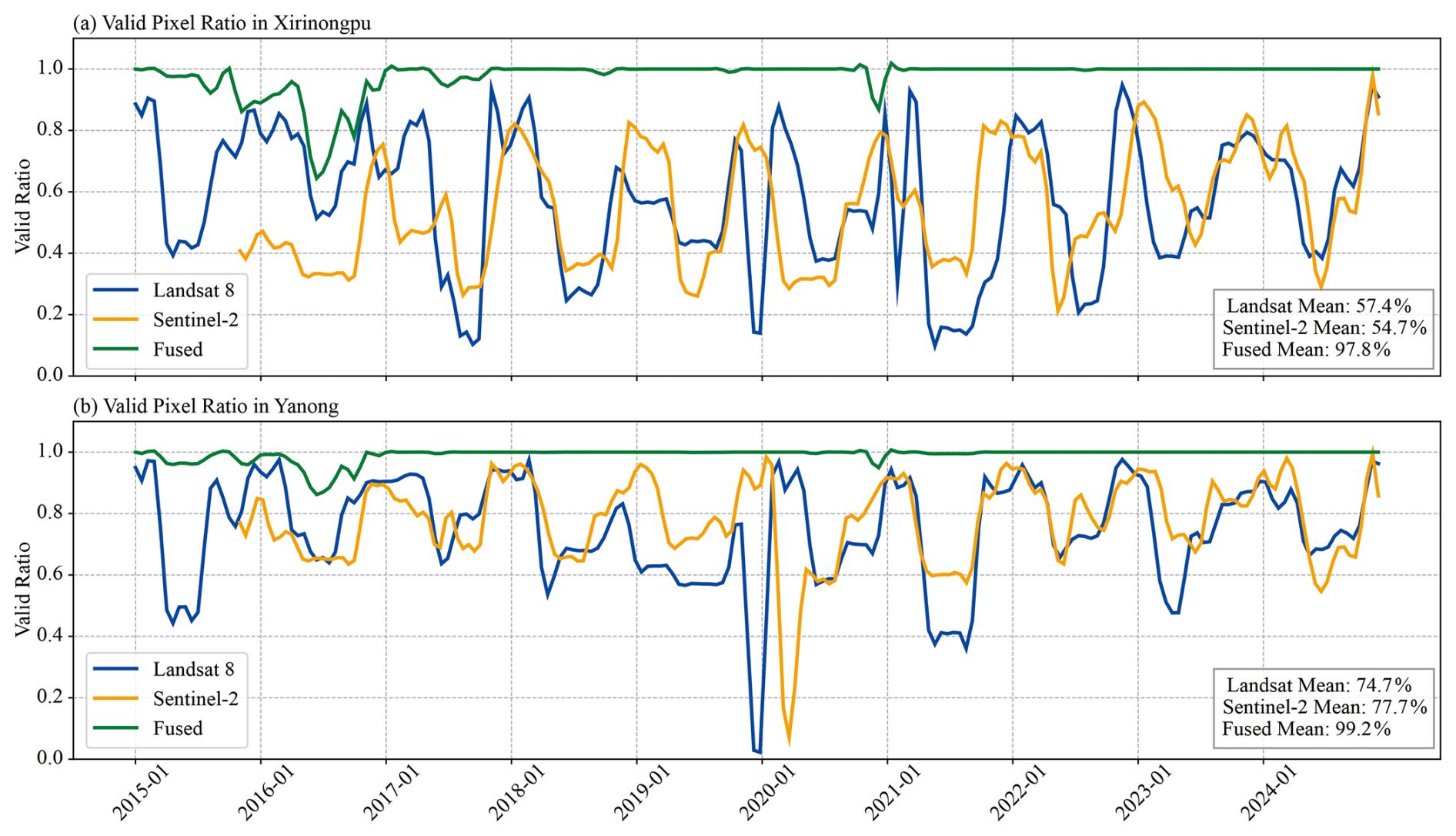
Figure 3 (a) Xirinongpu Glacier; (b) Yanong Glacier – proportion of valid pixels before and after fusion.

Figure 4 shows the spatial distribution of valid observation months before and after fusion over the representative Yanong and Xirinongpu glaciers. The fused product achieves near-complete temporal coverage in both areas: the vast majority of pixels have a full set of 120 monthly velocity values over the decade. For Yanong, the fused mean number of valid months is 117.8, compared with 76.3 for Landsat and 67.6 for Sentinel-2. For Xirinongpu, the fused mean reaches 117.2, versus 68.6 (Landsat) and 58.6 (Sentinel-2). Overall, the fusion method delivers substantial improvements in temporal availability.

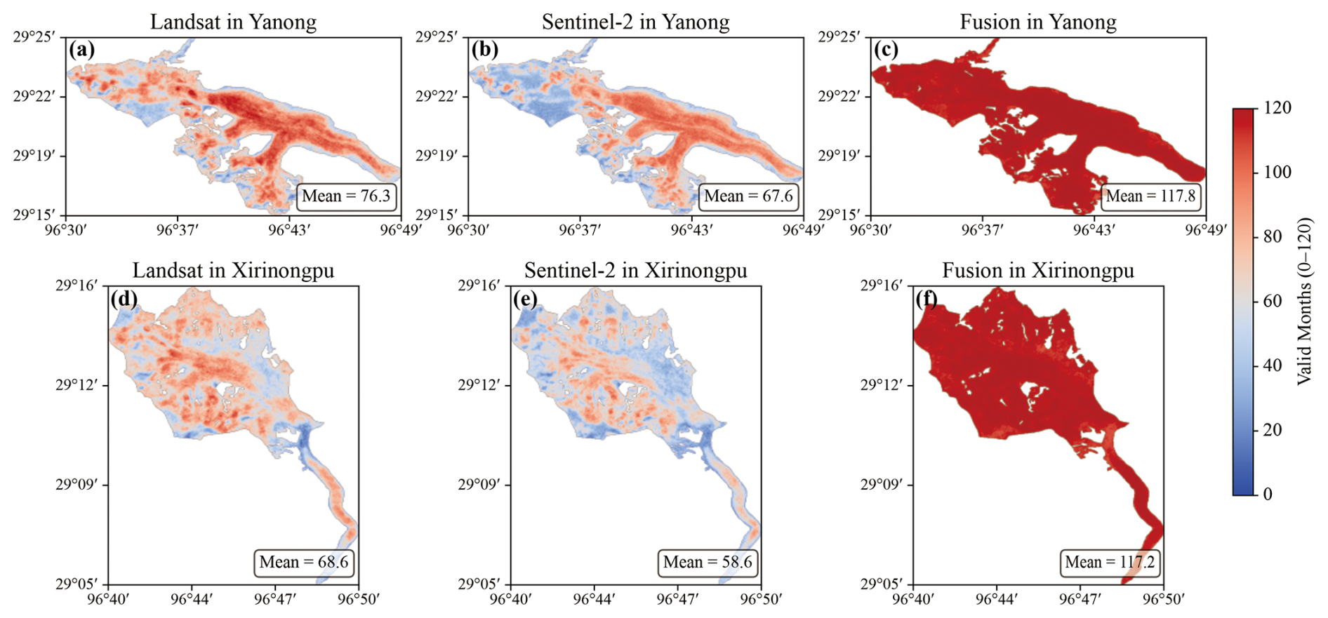
Figure 4 (a–c) Landsat / Sentinel-2 / fused velocity results: number of valid months on the Yanong Glacier; (d–f) Landsat / Sentinel-2 / fused velocity results: number of valid months on the Xirinongpu Glacier.

Figure 5 presents the RMSD-based image smoothness assessment for Yanong and Xirinongpu glaciers. RMSD was calculated as the root-mean-square deviation of each monthly velocity map from the 2015–2024 mean fused velocity map. This metric has the same unit as velocity and therefore provides a direct measure of the magnitude of deviation from the reference velocity field. A lower RMSD indicates that the monthly velocity map deviates less from the reference field and exhibits smoother and more stable image characteristics.

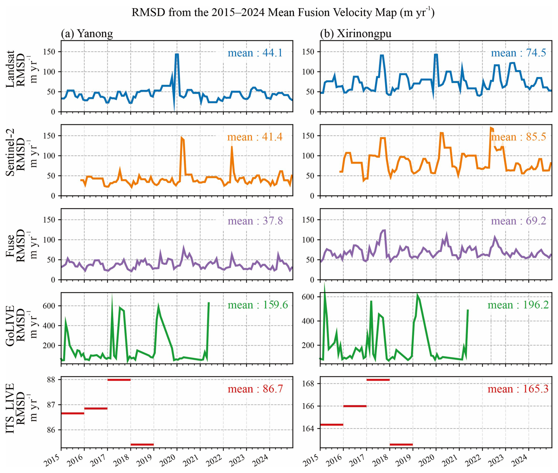
Figure 5 RMSD-based image smoothness assessment for the Landsat, Sentinel-2, fused, GoLIVE, and ITS_LIVE velocity products over (a) Yanong Glacier and (b) Xirinongpu Glacier. RMSD was calculated as the root-mean-square deviation of each monthly velocity map from the 2015–2024 mean fused velocity map within each glacier mask. GoLIVE and ITS_LIVE are shown only for the periods available in the corresponding datasets.

Over Yanong Glacier, the fused product has a mean RMSD of 37.8 m yr⁻¹, lower than Landsat (44.1 m yr⁻¹) and Sentinel-2 (41.4 m yr⁻¹), and much lower than GoLIVE (159.6 m yr⁻¹) and ITS_LIVE (86.7 m yr⁻¹). Over Xirinongpu Glacier, the fused product also shows the lowest mean RMSD, with a value of 69.2 m yr⁻¹, compared with Landsat (74.5 m yr⁻¹), Sentinel-2 (85.5 m yr⁻¹), GoLIVE (196.2 m yr⁻¹), and ITS_LIVE (165.3 m yr⁻¹). These results indicate that the fused velocity maps have lower deviations from the reference velocity field, suggesting improved image smoothness and reduced local fluctuations compared with the pre-fusion optical products and the two external datasets.

In sum, the proposed multi-source fusion not only enhances spatial completeness and temporal continuity, but also reduces RMSD from the reference velocity field, indicating improved image smoothness and providing a more stable basis for subsequent spatiotemporal modeling and change detection.

4.2 Uncertainty analysis

Figure 6 presents the temporal evolution of monthly velocity-uncertainty estimates in stable areas for Landsat, Sentinel-2, the fused product, GoLIVE, and ITS_LIVE. The fused product's E_off remains consistently low with relatively steady fluctuations; its mean uncertainty is 18.2 m yr⁻¹, markedly below the glacier-wide mean velocities and better than the pre-fusion Landsat (25.5 m yr⁻¹) and Sentinel-2 (21.9 m yr⁻¹) results, substantially lower than GoLIVE (116.9 m yr⁻¹), and slightly higher than the annual-scale ITS_LIVE (11.0 m yr⁻¹). Overall, the proposed multi-source fusion performs well not only in spatial completeness and continuity but also in uncertainty within stable zones, indicating strong practical utility and potential for broader application.

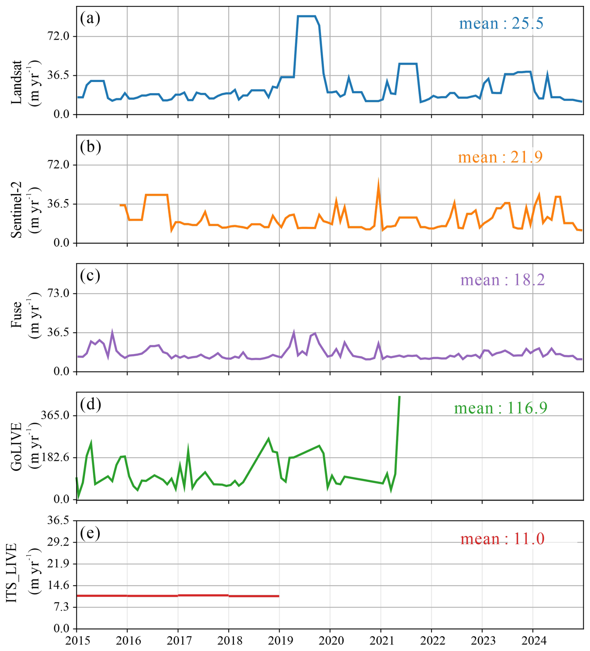
Figure 6 (a) Landsat velocity uncertainty; (b) Sentinel-2 velocity uncertainty; (c) Fused velocity uncertainty; (d) GoLIVE dataset uncertainty; (e) ITS_LIVE dataset uncertainty.

Figure 7 presents the uncertainty analysis results for the Landsat-derived velocities, Sentinel-2-derived velocities, UAV-derived velocities, and fused velocities within the UAV survey area. The results show that the fusion method effectively reduces uncertainty relative to the individual optical products. However, a substantial gap still remains between the fused results and the UAV-derived reference. This indicates that, although data fusion can reduce errors to some extent, it still does not achieve the accuracy level of high-precision UAV observations. Moreover, uncertainty estimates based on stable-ground pixels and subsequently propagated to glacier surfaces have inherent limitations. Therefore, the uncertainty obtained from the present data-fusion framework is likely to be underestimated.

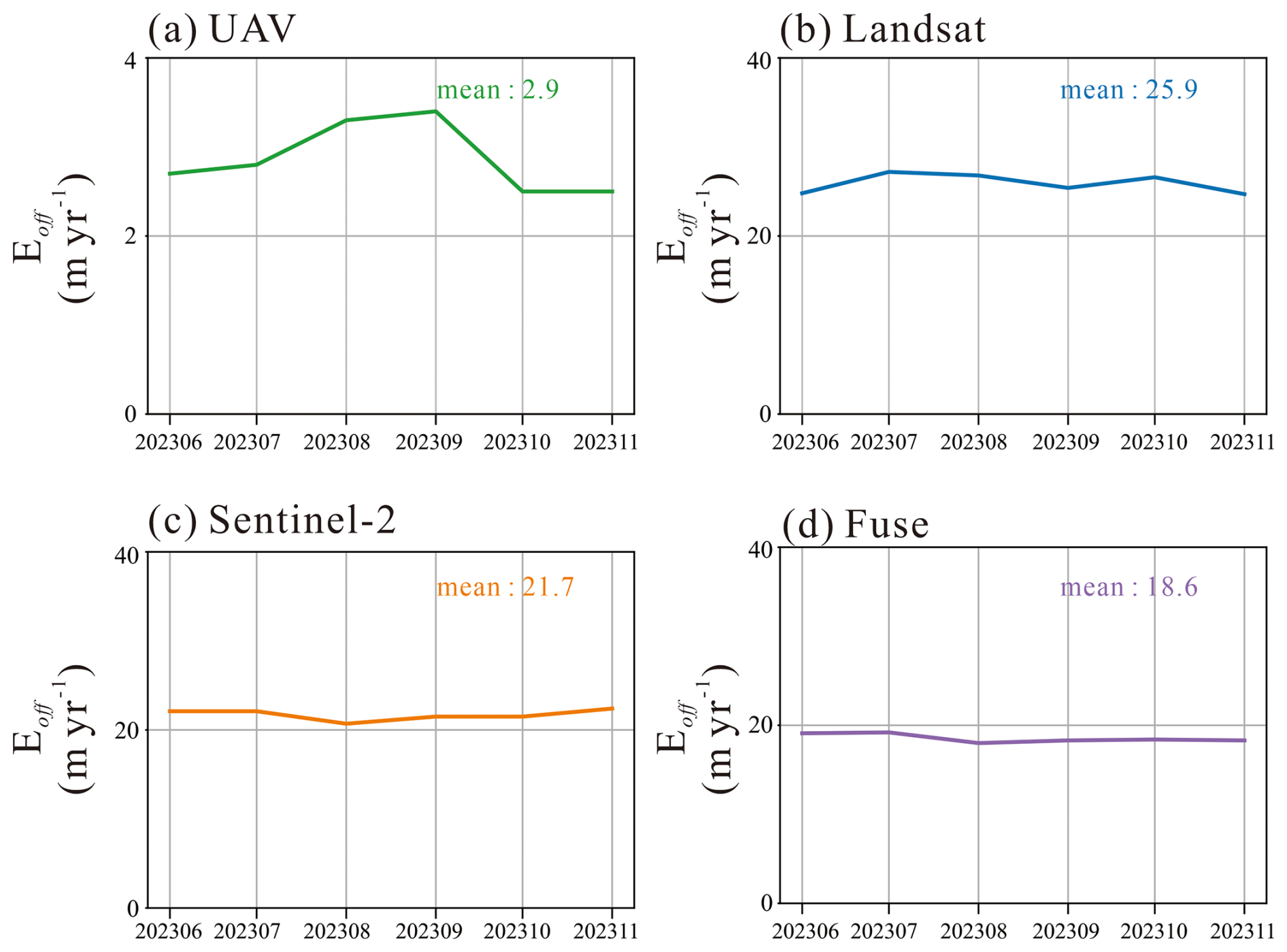
Figure 7 Uncertainty analysis of the four velocity products within the UAV survey area from June to November 2023: (a) UAV-derived velocity uncertainty; (b) Landsat-derived velocity uncertainty; (c) Sentinel-2-derived velocity uncertainty; and (d) fused velocity uncertainty.

4.3 Spatial patterns of glacier surface velocity and controlling factors

From 2015 to 2024, glacier surface velocity in the Kangri Karpo region shows the canonical “fast center, slow margins” spatial pattern (Fig. 8), with annual-mean maxima concentrated near the equilibrium line. The spatial organization of velocity is closely tied to glacier morphology. To identify the primary controls, we analyze glacier attributes-size (area), slope, and aspect-using correlation analysis, centerline profiles, and cluster-based grouping to assess their roles in shaping glacier dynamics.

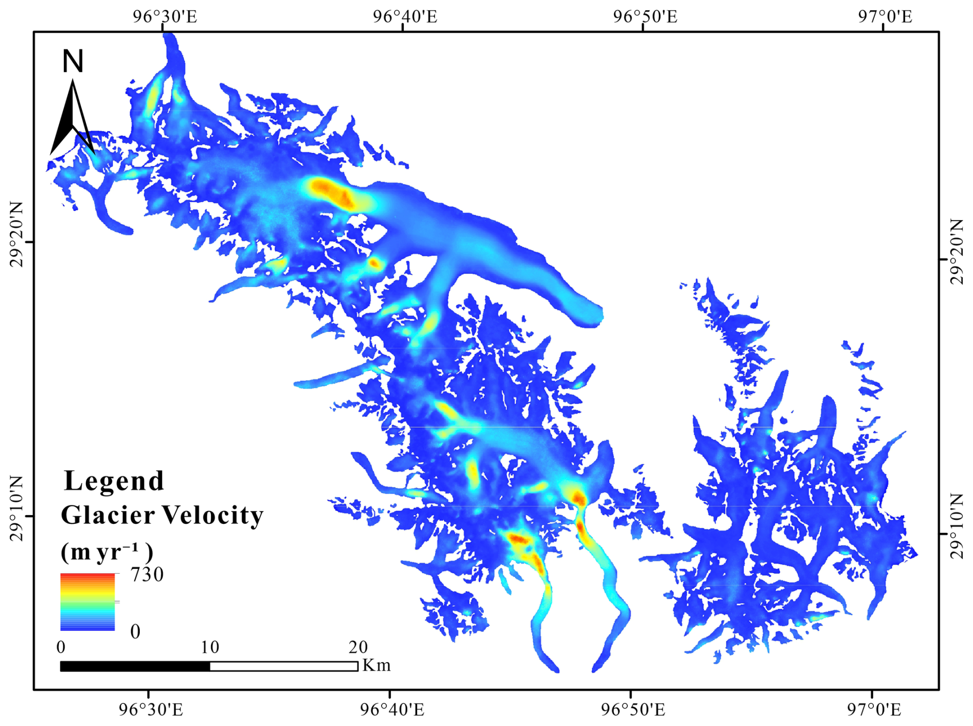
Figure 8 Mean glacier surface velocity in the Kangri Karpo region (2015–2024).

To examine how glacier size affects surface velocity in the Kangri Karpo region, we used total glacier area (km²) as the independent variable and the decadal mean surface velocity as the dependent variable, and performed a correlation analysis on log-transformed variables. As shown in Fig. 9, glacier area and mean surface velocity exhibit a moderate positive correlation (Pearson r=0.53, p<0.05), indicating a statistically significant tendency for velocity to increase with area. The presence of outliers suggests that factors beyond area – such as slope and aspect – also influence glacier speed.

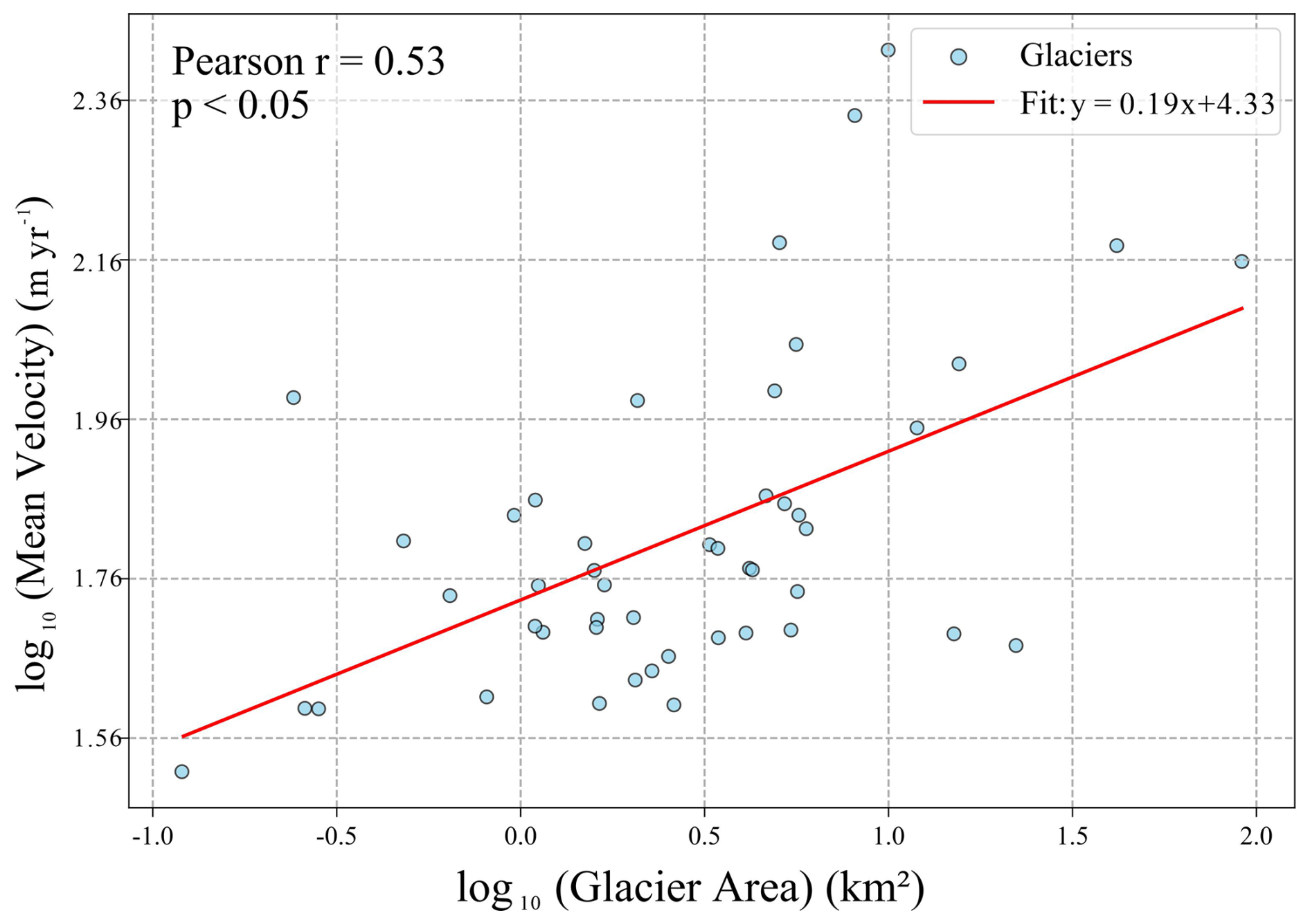
Figure 9 Correlation between glacier area and velocity. Blue points denote glaciers in the study area; the red solid line is the fitted regression; axes are logarithmic.

To further assess the role of slope, we conducted a pixel-level slope–velocity analysis along the main centerlines of two representative glaciers, Yanong and Xirinongpu (see Fig. 10).

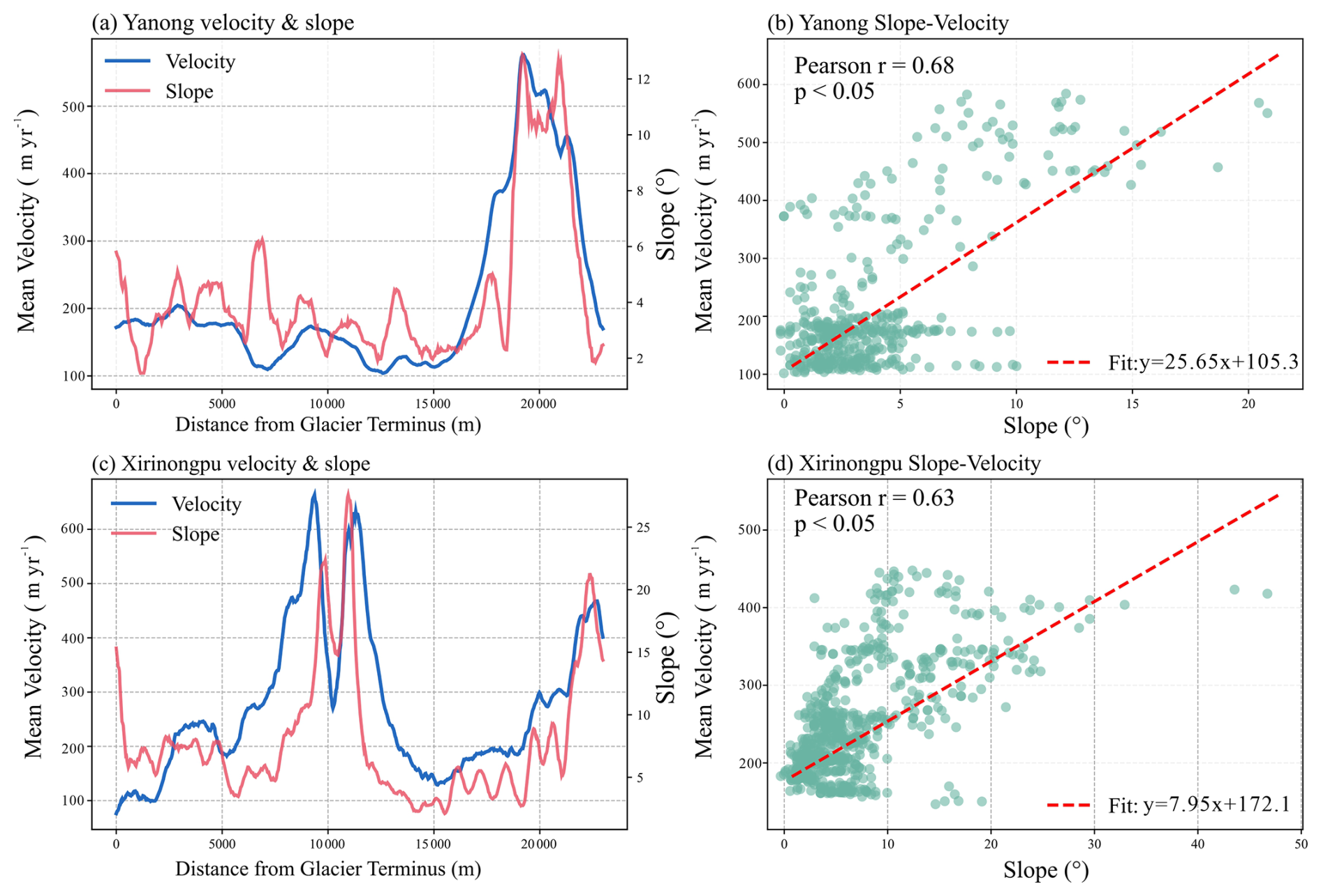
Figure 10 (a, c) Variations of glacier surface velocity and slope along the centerlines of the Yanong and Xirinongpu glaciers. Blue curve: velocity; red curve: slope. (b, d) Scatterplots of velocity versus slope for all pixels within the Yanong and Xirinongpu glacier masks; red dashed line: linear fit of the slope-velocity relationship.

Compared with regional mixed analyses, the centerline approach effectively controls for differences in glacier size, morphology, and aspect, helping reveal the intrinsic slope–velocity relationship within a single glacier. Along the Yanong centerline (0–23 000 m), both velocity and slope show phased rises and falls, with marked co-variation in several segments. Scatterplot regression indicates a significant positive correlation between slope and surface velocity (Pearson r=0.68, p<0.05). Xirinongpu exhibits similar behavior, with a correlation of r=0.63 (p<0.05); the fitted linear model has a slope coefficient of 15.42 and an intercept of 153.3. These results pass significance tests and suggest that, within an individual glacier, increasing slope promotes higher surface velocity, consistent with glacier-flow theory: a steeper centerline increases the downslope gravitational component, enhancing basal sliding and viscous deformation and thereby accelerating flow.

To systematically examine the relationship between surface velocity and aspect across the Kangri Karpo glaciers, we first grouped major glaciers by morphological attributes (e.g., area and slope) using k-means clustering (Fig. 11a). Clustering serves to control the confounding effects of area and slope when analyzing aspect–velocity links. The glaciers were partitioned into three clusters; because Cluster 3 contains only two glaciers and lacks statistical power, subsequent analyses focus on Clusters 1 and 2.

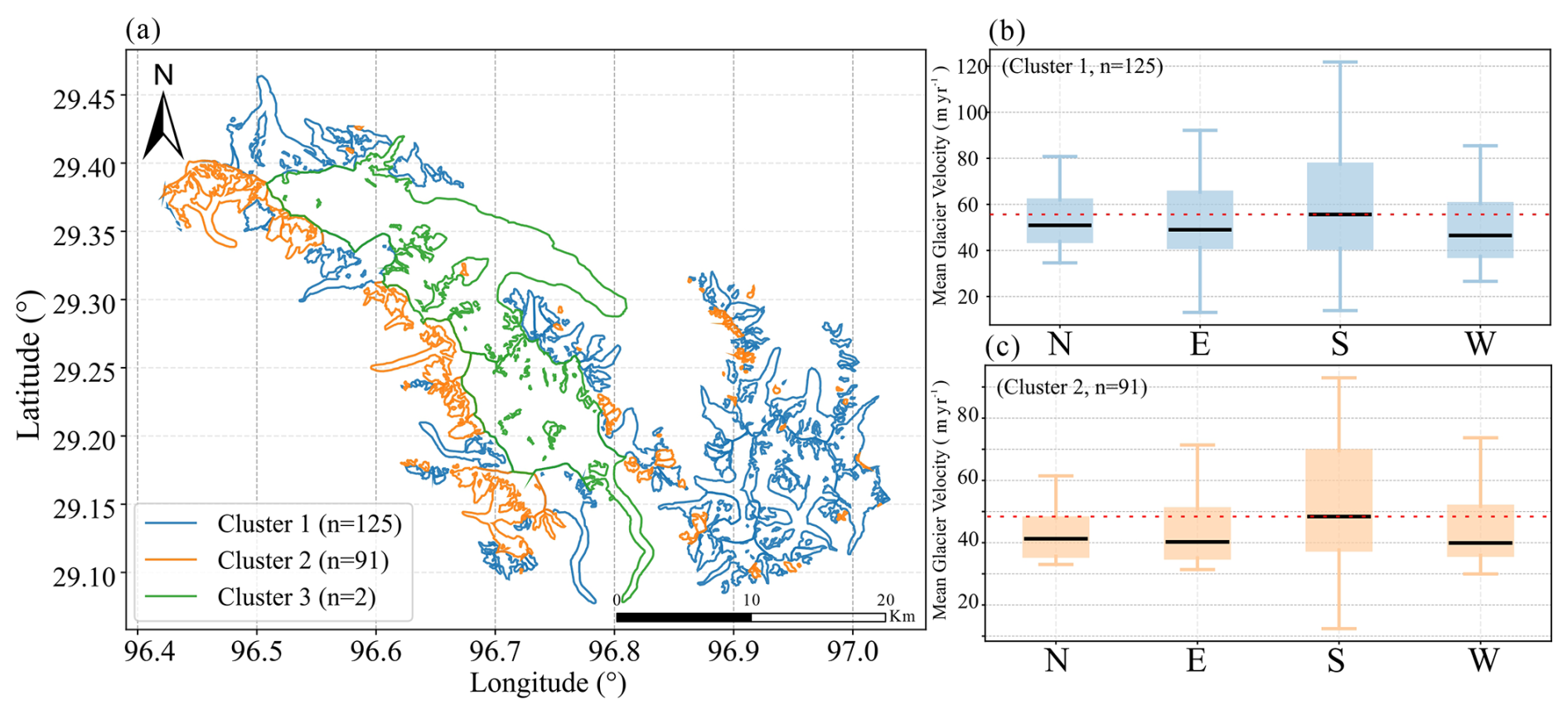
Figure 11 (a) K-means clustering (K=3) of all glaciers in the study area based on area and slope. (b, c) Boxplots of velocity by aspect for glaciers in Cluster 1 and Cluster 2, respectively. The box top is the upper quartile, the black line is the median, and the box bottom is the lower quartile; the red dashed line marks the median velocity of the aspect with the highest median.

Building on aspect-based grouping, we summarized glacier surface velocities across aspect classes. As shown in Fig. 10b and c, mean velocities differ by aspect (N, E, S, W), with both Cluster 1 and Cluster 2 exhibiting systematically higher velocities on south-facing S glaciers, and lower velocities on north-, east-, and west-facing glaciers. This pattern is consistent with the southeastern Tibetan Plateau's monsoonal climate: during summer, warm–moist air masses from the south enhance snowfall and meltwater supply on S-facing glaciers, favoring accumulation and flow. Stronger insolation on S-facing slopes also increases surface energy input, promoting basal or surface melt and further accelerating flow. By contrast, N/E/W aspects receive less moisture and energy due to shading and airflow blocking, yielding lower velocities. These features highlight the coupled control of regional climate and topography on glacier motion.

In sum, glacier surface velocity in the Kangri Karpo region reflects the combined influence of multiple topographic factors. Statistically, glacier area is positively correlated with mean surface velocity, implying faster flow for larger glaciers. Centerline analyses further confirm the key regulatory role of slope within individual glaciers. Aspect-based results after clustering show that, under Indian monsoon influence, S-facing glaciers move significantly faster than other aspects, revealing the joint effects of regional climate and terrain. Overall, glacier size, slope, and aspect jointly shape the spatial pattern of surface velocity and are key determinants for understanding dynamical change on the Plateau.

4.4 Intra-annual variability of glacier surface velocity

To characterize intra-annual variability in the Kangri Karpo region, we extracted monthly velocities from the 2015–2024 fused product and averaged each calendar month across years to derive a climatological annual cycle (Fig. 12). The resulting series shows a clear seasonal signal: velocities are relatively low in January–March, increase from March onward, reach a first peak in May, remain comparatively stable during summer, rise again to a second peak in October, and then decline. This indicates a bimodal intra-annual velocity pattern in the study region.

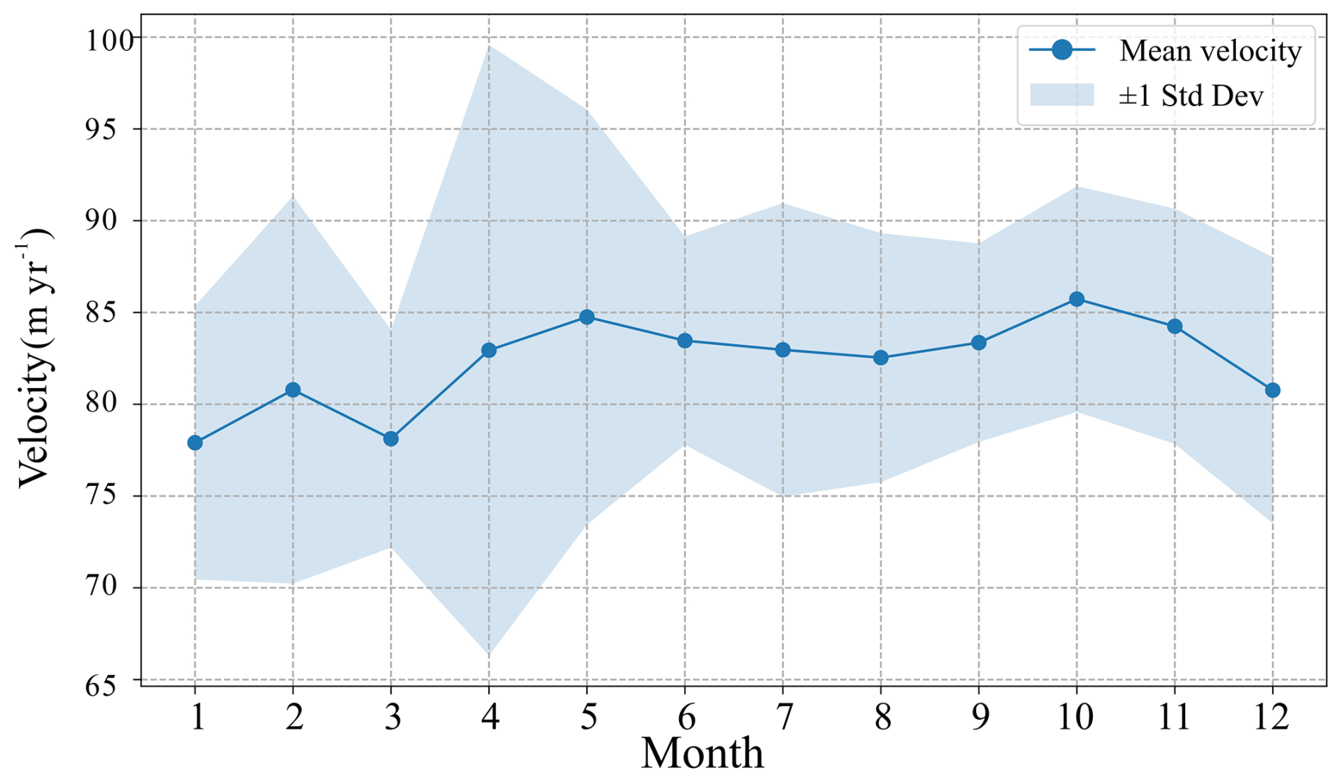
Figure 12 Monthly mean velocity (2015–2024). Blue points and line indicate the monthly means and their variation; blue shading shows ±1 standard deviation.

This bimodal pattern is broadly consistent with process-based interpretations proposed for temperate/maritime glaciers, in which seasonal changes in subglacial drainage efficiency modulate basal sliding. In particular, early-season meltwater and rainfall inputs may enhance sliding under a relatively inefficient distributed drainage system, whereas subsequent drainage-system evolution toward more efficient channelized flow may reduce mean basal water pressure and limit velocities later in the melt season; partial re-closure or renewed pressurization may contribute to a later-season acceleration. Similar seasonal acceleration behaviour, including autumn acceleration, has also been reported for mountain glaciers in other regions (e.g., Nanni et al., 2023). However, we emphasize that the present study does not include direct observations of subglacial hydrology, and therefore this interpretation should be viewed as plausible rather than diagnostic.

The standard-deviation envelope in Fig. 11 further suggests month-dependent interannual variability. Standard deviations are larger in April–May, when seasonal acceleration initiates, indicating stronger year-to-year differences in the timing and magnitude of acceleration. By contrast, variability is comparatively smaller from June to the following March. Taken together, these results indicate a clear seasonal velocity response in the Kangri Karpo region, with a recurrent bimodal intra-annual structure.

4.5 Interannual variability and long term trends

Using the monthly fused glacier-velocity images for 2015–2024, we applied linear regression to each pixel within the study mask in the Kangri Karpo region to quantify velocity trends (units: m yr⁻¹ per decade), thereby revealing the direction and magnitude of decadal changes in glacier surface speed (Fig. 13).

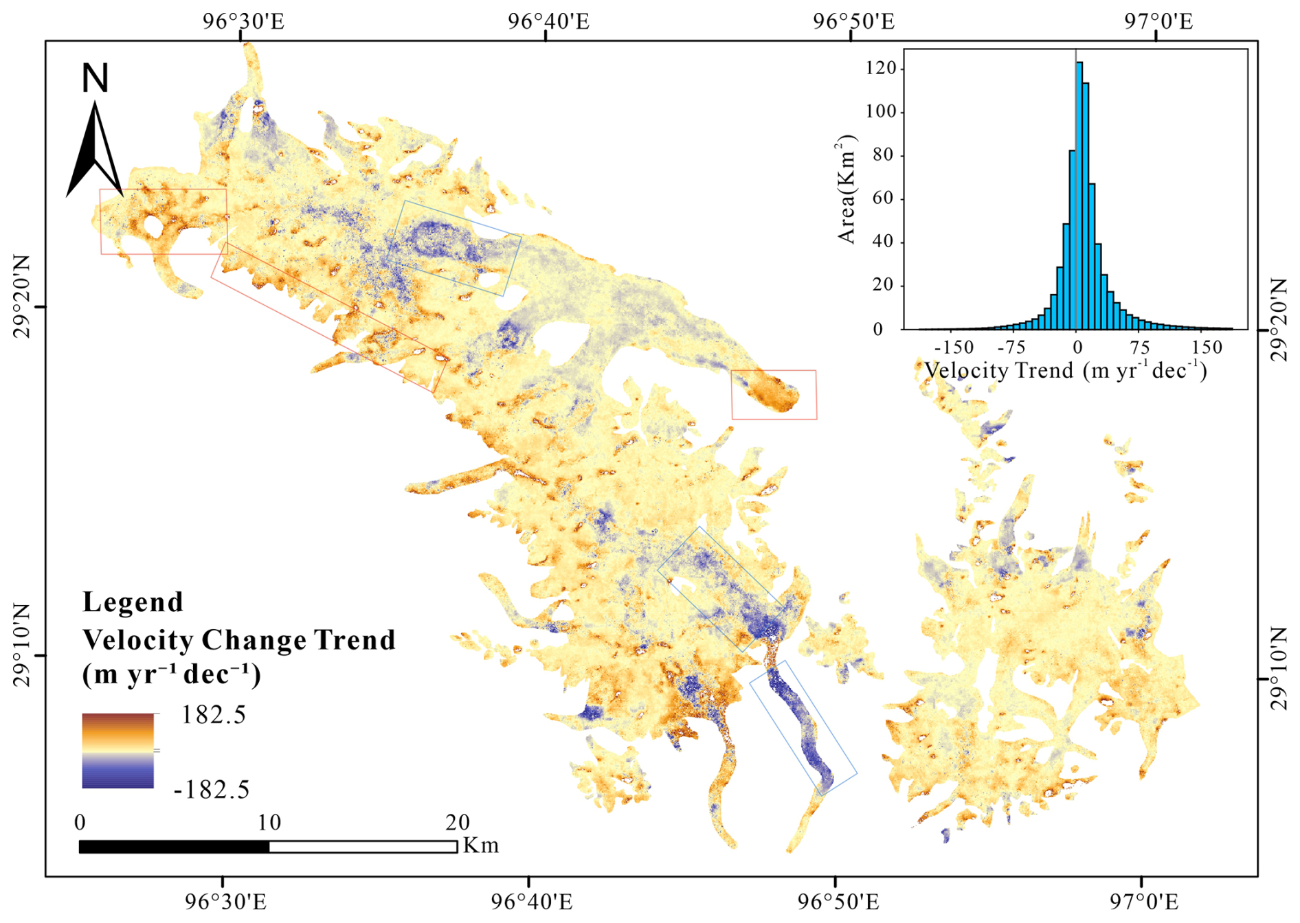
Figure 13 Main panel: per-pixel decadal trend in glacier surface velocity within the study mask (units: m yr⁻¹ per decade). Warmer (redder) colors indicate stronger acceleration; cooler (bluer) colors indicate stronger deceleration. Red and blue boxes highlight representative accelerating and decelerating areas. Upper-right inset: area-weighted distribution of trend values.

The results show pronounced differences in decadal trends among major glaciers. On the two largest – Yanong and Xirinongpu – broad swaths of negative trends (blue boxes in Fig. 13) indicate pronounced slowdowns, whereas the Yanong terminus exhibits marked acceleration, likely related to the influence of a proglacial lake. By contrast, smaller glaciers in the region (red boxes) display relatively clear acceleration.

Area-based statistics of the trend map (Fig. 13) approximate a normal distribution, with most pixels falling between −36.5 and +36.5 m yr⁻¹ per decade, implying generally modest changes. The median trend is slightly positive, indicating a weak, basin-wide acceleration during 2015–2024.

To further characterize interannual variability, we applied linear regression to the 2015–2024 velocity series and summarized each glacier's (>1 km²) trend together with its mean aspect. Unlike Fig. 13, which shows the direction and magnitude of pixel-wise trends without significance classification, Fig. 14 presents the glacier-level trend analysis with statistical significance testing. Figure 14 presents the multi-year trends of glacier surface velocity and the distribution of mean aspects across the Kangri Karpo region.

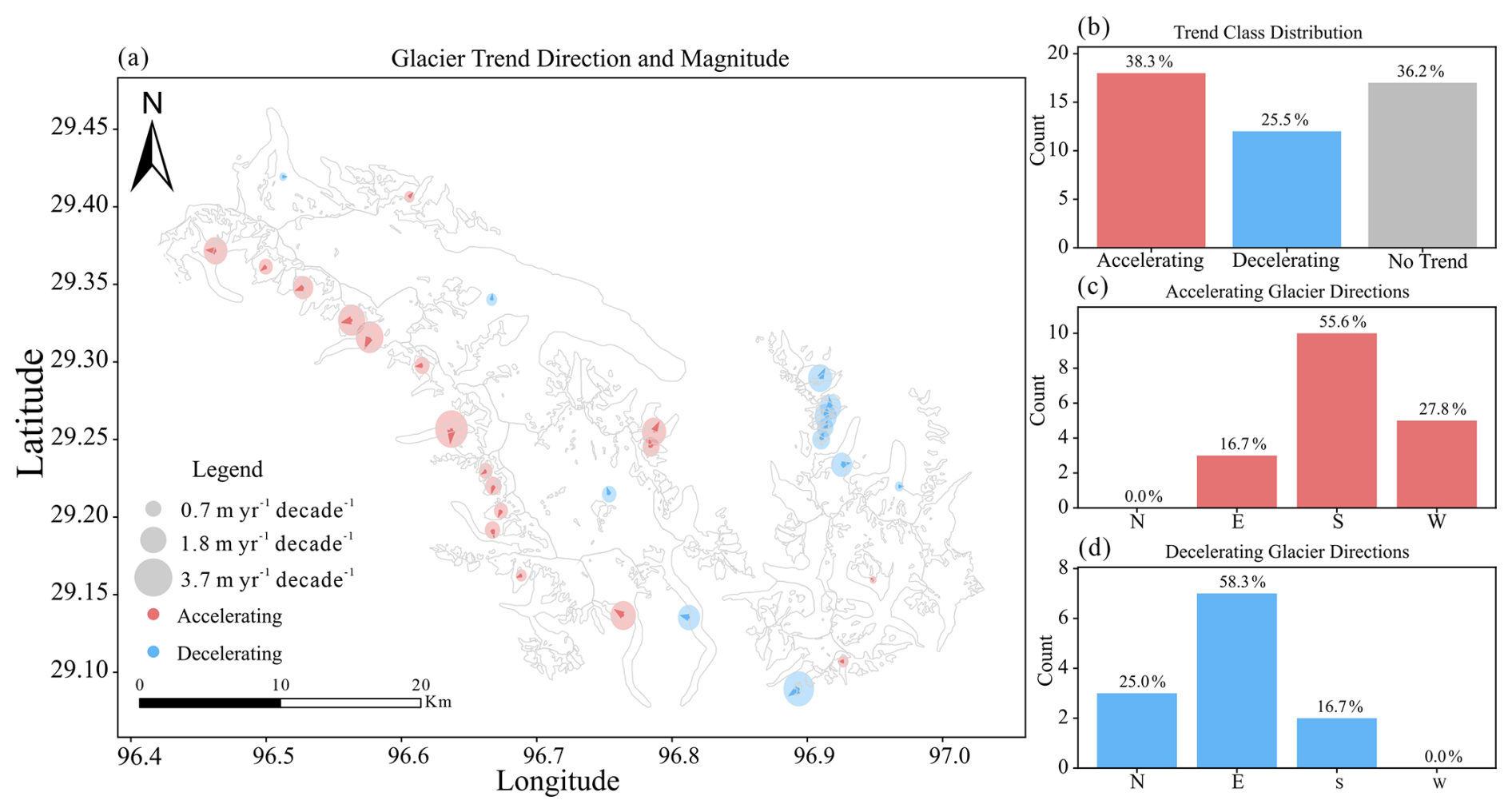
Figure 14 (a) Schematic map of glacier velocity trends across the study area. Circle color indicates trend direction (acceleration/deceleration); circle size indicates trend magnitude; the arrow inside each circle shows the glacier's mean aspect. Glaciers without circles exhibit no significant trend. (b) Counts and percentages of glaciers by trend class (significant acceleration / significant deceleration / no significant change). (c) Counts and percentages of significantly accelerating glaciers by aspect. (d) Counts and percentages of significantly decelerating glaciers by aspect.

Spatially, accelerating and decelerating glaciers show distinct patterns. Some accelerating glaciers are concentrated in the western and central sectors of the region, whereas decelerating glaciers are relatively clustered in the eastern sector and parts of the central area. Accelerating glaciers predominantly exhibit a southwest–northeast principal flow orientation, while decelerating glaciers are more clearly aligned east–west, indicating differences in multi-year trends by flow orientation.

The three bar charts on the right further summarize change characteristics by glacier type. Trend-class distributions show that ∼38.3 % of glaciers exhibit significant acceleration, 25.5 % show significant deceleration, and 36.2 % have no significant multi-year trend (based on the glacier-level linear regression test, p≥0.05). By mean aspect, significantly accelerating glaciers are concentrated on south-facing (50.0 %) and west-facing (27.8 %) slopes, whereas significantly decelerating glaciers are dominated by east-facing (58.3 %) and north-facing (25.0 %) slopes. These results indicate clear directional differences in recent glacier dynamics, likely governed by a combination of regional topography, snow/ice supply, and climatic conditions.

Figure 15 further presents monthly multi-year velocity trends (2015–2024) and their 95 % confidence intervals for different glacier types in the Kangri Karpo region: the upper panel shows significantly accelerating glaciers by month, and the lower panel shows significantly decelerating glaciers by month. The y axis is the decadal trend in velocity (m yr⁻¹ per decade). Line segments above the bars indicate the 95 % confidence interval of the monthly mean trend.

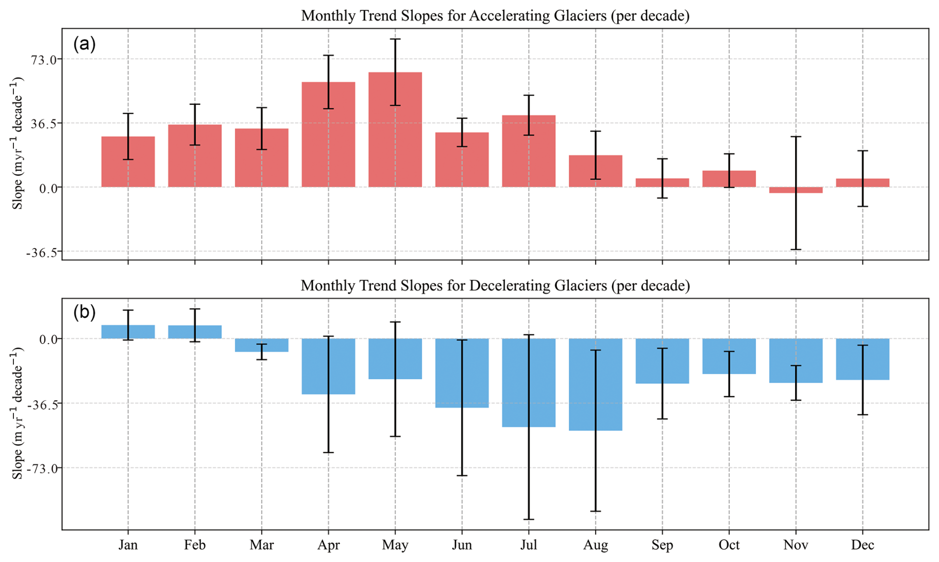
Figure 15 (a, b) Monthly velocity trends for significantly accelerating/decelerating glaciers; black lines above the bars indicate the 95 % confidence interval of the monthly mean trend.

From the accelerating-glacier subset, acceleration concentrates in late spring to early summer: April and May exhibit the largest multi-year trends (∼54.7–73.0 m yr⁻¹ per decade), with confidence intervals excluding zero, indicating strong significance. A plausible explanation is the recent advance of the melt season in southeastern Tibet (Li et al., 2025; Wu et al., 2022), during which a distributed subglacial drainage system has high storage and low efficiency, elevating basal water pressure and enabling earlier meltwater access to the bed – thus promoting early-season acceleration.

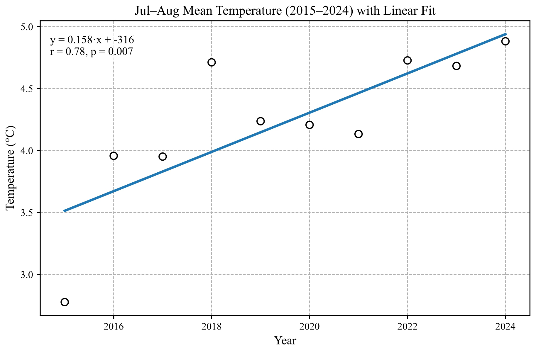
Figure 16 ERA5-Land temperature trends for July and August, 2015–2024. Circles denote each year's mean temperature; the blue solid line is the linear fit.

For decelerating glaciers, slowdown concentrates in summer – especially July–August – when trends fall below −54.7 m yr⁻¹ per decade, indicating the strongest deceleration. A plausible cause is the marked rise in July–August air temperature (ERA5-Land; Fig. 16), which intensifies mass loss, while the subglacial drainage system is channelized and efficient; glacier motion is then dominated by creep, so negative mass balance drives a pronounced deceleration peak in July–August.

By size, accelerating glaciers are generally smaller. Because creep is weaker in small glaciers, early-season hydrological acceleration can outweigh the year-scale mass deficit, making acceleration more common. Large glaciers are more strongly governed by creep, with mass balance the primary control on speed; hence they tend to decelerate in summer and over multi-year scales, consistent with the warming-driven, widespread slowdown across High Mountain Asia (Dehecq et al., 2019).

In summary, the “April–May acceleration vs. July–August deceleration” pattern reflects the joint effects of an advanced melt season (hydrological forcing) and mass balance. This broadly accords with current understanding, while highlighting that for some glaciers, early-season meltwater acceleration can exceed the decelerating influence of mass loss.

4.6 Limitations and future directions

A key limitation of this study is that the UAV reference data used to calibrate the fusion weights cover only a relatively small area near the Yanong Glacier terminus, rather than the full range of glacier and terrain conditions across the Kangri Karpo region. Although this UAV subset includes heterogeneous conditions, such as fast-flowing trunk ice, slower marginal zones, debris-covered and clean-ice surfaces, and observations spanning the ablation season to the early accumulation period, it does not fully encompass the broader diversity of aspect, slope, surface characteristics, glacier type, and seasonal states represented in the entire study area. Therefore, the present weighting scheme implicitly assumes that the relative performance of Landsat, Sentinel-1, and Sentinel-2 derived from this limited reference area is transferable to other glaciers and time periods, which may not always hold. This limitation should be kept in mind when interpreting the regional applicability of the fused product. Future work should therefore aim to develop spatiotemporally adaptive weighting strategies, for example by calibrating weights separately for different topographic settings, surface conditions, glacier types, and seasons, and by incorporating additional high-accuracy reference data from multiple glaciers and periods.

In addition, differences in sensor revisit cycles (Landsat ≈16 d; Sentinel-1 ≈12 d; Sentinel-2 ≈10 d) preclude strict month-to-month alignment, producing baseline-length mismatches, temporal overlap, and temporal smoothing that inevitably introduce additional uncertainty into the nominal monthly velocity series. Although glacier displacement was always divided by the exact temporal separation of each image pair, the resulting products should therefore be interpreted as nominal monthly interval-mean velocities rather than strictly calendar-month velocities. This limitation is particularly relevant for the analysis of intra-annual variability, because irregular and overlapping baselines may blur short-term temporal signals. Future work should explore regularized velocity time-series approaches that explicitly reconcile overlapping image-pair baselines, such as the framework proposed by Charrier et al. (2025), in order to generate temporally more rigorous and directly comparable glacier-velocity series.

Future work can proceed along two lines: (i) introduce spatiotemporally adaptive weighting – via stratified calibration or modeling conditioned on topography, surface texture, and acquisition geometry – to improve applicability over larger areas and longer periods; and (ii) standardize or assimilate time intervals by mapping multi-sensor displacements/velocities to a “standard month” framework to reduce baseline-induced biases. With higher-resolution, higher-cadence observations continuing to emerge, these refinements should substantially enhance the method's generalizability and support broader multi-sensor fusion.

5 Conclusions

This study proposes and implements a high-spatial-resolution glacier surface-velocity retrieval method based on multi-sensor data fusion, and produces monthly velocity products for the Kangri Karpo region for 2015–2024. Relative to existing large-area public datasets, our products markedly improve spatial resolution and enhance the detectability of small mountain glaciers. Compared with single-sensor inputs prior to fusion, the fused results increase the proportion of valid pixels by ∼50 %, add ∼50 valid months per pixel over the decade, and improve spatial smoothness – demonstrating that the method effectively mitigates single-source limitations under complex mountain conditions.

In spatial terms, glacier surface velocity during 2015–2024 exhibits the canonical “fast center, slow margins” pattern: multi-year mean maxima exceed 700 m yr⁻¹, whereas values in lower reaches and most tributaries are generally <100 m yr⁻¹. Regarding attribute controls, Pearson correlation analysis indicates statistically significant but moderate associations of velocity with glacier area, slope, and aspect: larger glaciers tend to flow faster; within individual glaciers, velocity is more strongly correlated with slope; and after accounting for area and slope, south-facing glaciers are slightly faster than glaciers of other aspects.

Seasonally, the series shows a clear cycle: peaks occur near the onset and end of the melt season, with persistently elevated speeds throughout the melt period. Interannually, most pixelwise decadal trends fall within −36.5 to +36.5 m yr⁻¹ per decade, indicating generally modest changes; the median trend is slightly positive, implying weak regional acceleration during 2015–2024. By significance class, ∼38.3 % of glaciers accelerate significantly, 25.5 % decelerate significantly, and 36.2 % show no significant trend (p≥0.05). By aspect, significant acceleration is concentrated on south- (50.0 %) and west-facing (27.8 %) glaciers, whereas significant deceleration is dominated by east- (58.3 %) and north-facing (25.0 %) glaciers. Month-resolved interannual trends show acceleration mainly in April–May (∼54.7–73.0 m yr⁻¹ per decade), likely reflecting earlier melt-season onset and meltwater-driven speed-up; deceleration concentrates in July–August ($\le -\mathrm{54.7}$ m yr⁻¹ per decade), likely reflecting mass-loss-driven slow-down.

These spatiotemporal patterns likely reflect interactions among glacier mass balance, subglacial hydrologic evolution, and regional climate (e.g., monsoon forcing). However, the specific drivers merit further process-based analysis integrating mass-balance observations and hydro-climatic factors.