Inferring subglacial topography using physics informed machine learning constrained by two conservation laws

Subglacial topography beneath the Greenland Ice Sheet is a fundamental control on its dynamics and response to changes in the climate system. Yet, it remains challenging to measure directly, and existing representations of the subglacial topography rely on a limited number of observations. Although the use of mass conservation and the development of BedMachine Greenland substantially improved the representation of the bed topography, this approach is limited to fast-flowing sectors and is less effective in regions with complex, alpine topography. As an alternative to traditional numerical methods, recent work has explored using Physics Informed Neural Networks (PINNs), constrained by only one physical law, to solve forward and inverse problems in ice sheet modeling. Building on this work, we assess three PINN frameworks constrained by distinct conservation laws, showing that PINNs informed with a single conservation law are not sufficient for regions with sparse measurements and complex topographies. To that end, we introduce a novel approach that involves coupling two conservation laws within a PINN framework to infer the subglacial topography and test this approach for three regions with distinct environments in Greenland. This PINN is trained with both the conservation of mass and an approximation of the conservation of momentum (the Shelfy-Stream Approximation), which allows us to simultaneously infer the ice thickness and basal shear stress using observations of ice velocities, surface elevation, surface mass balance, and ice thinning rates in a mixed inversion problem. We compare the predicted ice thickness to ground-truth ice-penetrating radar measurements of ice thickness, showing that the PINN informed with two conservation laws is capable of inferring ice thickness in sparsely surveyed regions. Furthermore, comparisons of predicted bed topographies with BedMachine Greenland show that this approach is capable of discovering new bed features in slower-moving regions and in regions of complex topography, highlighting its potential for better constraining the bed topography of the Greenland Ice Sheet.

1 Introduction

Approximately 58 and 7 m of sea level equivalent are sequestered in the Antarctic Ice Sheet and the Greenland Ice Sheet (GrIS), respectively (Morlighem et al., 2017; Morlighem et al., 2025; Morlighem et al., 2020; Morlighem, 2025; Pritchard et al., 2025), and they already contribute to global sea level rise at rates of 0.39 and 0.74 mm yr⁻¹, respectively (Otosaka et al., 2023). Despite an increase in the availability of remote sensing data and recent progress made in numerical ice sheet modeling (e.g., Nowicki et al., 2016; Goelzer et al., 2017, 2018; Nowicki et al., 2020; Seroussi et al., 2020, 2024), the uncertainty in the future mass balance of the ice sheets remains high (e.g., Aschwanden et al., 2021; Seroussi et al., 2020; Goelzer et al., 2020).

Among the sources of uncertainty, poorly constrained subglacial topography (or more simply, bed topography) remains one of the major factors affecting ice sheet model projections. While its impact at the ice sheet scale has not yet been rigorously quantified, Durand et al. (2011) showed that differences in the bed topography at resolutions greater than 2 km could lead to significant variations in ice sheet model behavior for regions prone to Marine Ice Sheet Instability (MISI). More recently, Castleman et al. (2022) reported that the uncertainty in Thwaites Glacier's contribution to sea level due to the bed topography alone may be as large 21.9 cm over the next 200 years. The ice discharge at the ice sheet margin and stability of the grounding line and calving fronts are often preconditioned by the bed topography, with retrograde bed slopes having the potential to induce rapid retreat through MISI (e.g., Schoof, 2012; Catania et al., 2018; Morlighem et al., 2019). In addition to controlling ice flow, the bed topography also influences the routing of subglacial water, which in turn affects basal sliding (e.g., Gagliardini et al., 2007; Schoof, 2010). Since the 1960s, ground-based and airborne ice-penetrating radars have been used to measure the ice thickness of the ice sheets, from which we can then obtain the bed elevation (e.g., Evans and Robin, 1966; Rutishauser et al., 2016; CReSIS, 2016; Paden et al., 2010). Yet, these observations are limited in spatial coverage with gaps reaching tens of kilometers in some areas of the ice sheet, thus not meeting the kilometer-scale spatial resolutions required by ice sheet models. Despite efforts to better constrain the bed topography through increased data acquisition (e.g., NASA's Operation IceBridge Paden et al., 2010), large uncertainties persist across many regions of the Antarctic and Greenland ice sheets.

Ice sheet models rely on indirect methods to resolve the bed topography between ice-penetrating radar-derived observations, which involve inferring the ice thickness (and subsequently the bed elevation) from observable ice sheet data. These observable data include surface elevation, ice velocities, surface mass balance, ice thinning rates, and sparse ice thickness measurements from ice-penetrating radar. Traditional indirect methods involve using geo-statistical methods like kriging (e.g., Bamber et al., 2001, 2013) or numerically inverting for ice thickness using mass conservation (e.g., Morlighem et al., 2011). A combination of these traditional methods culminated in the development of BedMachine Greenland (Morlighem et al., 2017; Morlighem et al., 2025) and BedMachine Antarctica (Morlighem et al., 2020; Morlighem, 2025), which are currently widely used by the cryosphere community. Yet, the mass-conserving approach of BedMachine is limited to fast-flowing sectors and is often challenging to apply in regions with sparse measurements and complex topography, such as the mountainous areas of Southeast Greenland.

Machine learning methods have risen as a promising new approach to improve upon existing representations of the bed and capture realistic bed topography features, with the ice thickness inversion framed as a “minimization problem” per the classification by Farinotti et al. (2017). However, standard machine learning methods may not necessarily account for the physical processes governing the dynamics of ice sheets and glaciers. Embedding prior knowledge, such as the fundamental conservation laws within a machine learning model architecture allows for the development of a robust framework (Raissi et al., 2019; Karniadakis et al., 2021). Such machine learning models, or neural networks, are called Physics-Informed Neural Networks (PINNs), which are designed to ensure that their predictions satisfy the governing physical principles (Raissi et al., 2019; Karniadakis et al., 2021). Within glaciology, PINNs were first used by Riel et al. (2021) to better understand the basal mechanics beneath glaciers. Since then, the literature on PINNs has grown (e.g., Riel and Minchew, 2023; Iwasaki and Lai, 2023; Jouvet, 2023; Cheng et al., 2024; Wang et al., 2025).

In this paper, we use PINNs to infer the ice thickness, and subsequently the bed topography, in sectors of the GrIS where traditional inversion methods (such as the mass-conserving approach of BedMachine) are less effective. Following Cheng et al. (2024), we solve a two-dimensional, mixed inverse problem in which both the ice thickness and basal friction are inferred for three glaciologically distinct regions in Greenland. Our experiments explore different configurations of physical constraints within the PINN framework: mass conservation alone, momentum conservation alone, and a coupled system incorporating both conservation laws. The PINNs for each experiment are implemented using the open-source Python package, Physics-Informed Neural Networks for Ice and CLimatE (PINNICLE, Cheng et al., 2025b). Our objective is to determine the PINN framework and the physical constraints that are most effective for improving on existing representations of the bed topography in sectors with complex, alpine topography and slower-moving sectors further inland that do not have a high density of ice thickness observations.

2 Methods

The overall approach outlined in this section builds on the framework described in Cheng et al. (2024). We only provide a brief overview of the general PINN framework and our methods specific to this study, and refer the reader to Cheng et al. (2024, 2025b) for further details.

2.1 General Framework

We initialize and train the PINNs with the Python package, PINNICLE (Cheng et al., 2025b). The PINN inputs are the spatial coordinates and the outputs are the state variables in the partial differential equations (PDEs) used to constrain PINN predictions. Following the architecture described in Raissi et al. (2019), the PINN learns a relationship between the input and output variables from both the training data and from the PDEs with the help of a loss function (or cost function), that describes the total error in PINN predictions, shown below:

$$\begin{array}{}\text{(1)}& \mathcal{L}={\mathcal{L}}_{\text{data}}+{\mathcal{L}}_{\mathit{\phi }},\end{array}$$

where ℒ_data is the data loss and ℒ_φ is the physical loss. Though the total loss can be defined in different ways (we refer the reader to Cheng et al. (2025b) for further details on loss function definitions), we use the mean squared error (MSE) to calculate the loss terms for this study. The data loss quantifies the misfit between PINN predictions and the training data. In particular, the PINN randomly selects a set of distinct spatial locations or “data points” within the region of interest and calculates the MSE between the PINN predictions and training data over these data points. The physical loss measures how well the PINN predictions satisfy the PDEs, thus serving as a soft constraint which enforces the physical laws. This is done by randomly selecting “collocation points” within the region of interest and calculating the MSE of the PDE residuals over these collocation points. During the training process, the PINN minimizes this loss function and updates its neural network coefficients accordingly, as illustrated in Fig. 1.

Our PINN framework (Fig. 1) uses 6 fully connected (“dense”) layers with 128 neurons each and a hyperbolic tangent activation function between layers. We use Adam optimization, a learning rate of $\mathrm{1.0}\times {\mathrm{10}}^{-\mathrm{4}}$, and train the PINN for 700 000 iterations, after which the predictions do not improve significantly and training is considered sufficient.

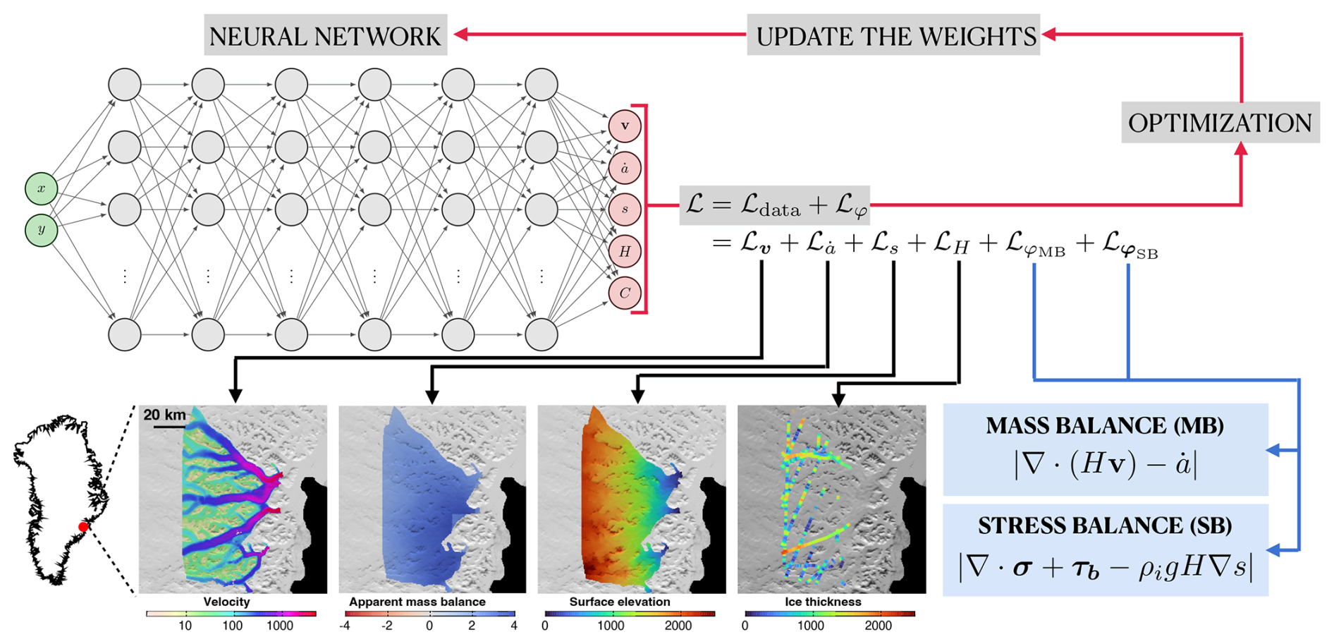
Figure 1 Illustration of the PINN framework, constrained by both mass conservation and momentum conservation, set up using the PINNICLE package. The inputs are the spatial coordinates and the outputs are the state variables of both PDEs. The loss function is comprised of data loss terms (black arrows) and physical loss terms (blue arrows).

2.2 Conservation Laws

Since we define our PINN output variables and select the training data according to the variables in the governing conservation laws, we first need to define the specific PDEs used for each of our experiments.

Let Ω⊂ℝ² be the two-dimensional region of interest. The two-dimensional, depth-integrated conservation of mass for ice, considered an incompressible fluid, reads:

$$\begin{array}{}\text{(2)}& {\displaystyle \frac{\partial H}{\partial t}}+\mathrm{\nabla }\cdot \left(H\mathit{v}\right)={\dot{M}}_{\mathrm{s}}-{\dot{M}}_{\mathrm{b}},\end{array}$$

such that for $\mathit{x}=(x,y{)}^{⊺}\in \mathrm{\Omega }$, H(x) is the ice thickness, $\mathit{v}\left(\mathit{x}\right)=(v_x,v_y{)}^{⊺}$ is the depth-integrated ice velocity, ${\dot{M}}_{\mathrm{b}}\left(\mathit{x}\right)$ is the basal melting rate, ${\dot{M}}_{\mathrm{s}}\left(\mathit{x}\right)$ is the surface mass balance, and $\partial H/\partial t$ is the ice thinning rate. Following Farinotti et al. (2009), we refer to the linear combination $\dot{a}\left(\mathit{x}\right)={\dot{M}}_{\mathrm{s}}\left(\mathit{x}\right)-{\dot{M}}_{\mathrm{b}}\left(\mathit{x}\right)-\partial H/\partial t$ as the “apparent mass balance”. Then, we denote the residual of the conservation of mass (or the mass balance residual), φ_MB(x), as

$$\begin{array}{}\text{(3)}& {\mathit{\phi }}_{\text{MB}}=\mathrm{\nabla }\cdot \left(H\mathit{v}\right)-\dot{a}.\end{array}$$

For the conservation of momentum, we use the Shelfy-Stream/Shallow-Shelf Approximation (SSA, Morland, 1987; MacAyeal, 1989). The residual of the conservation of momentum (or the stress balance residual), φ_SB(x), is expressed as follows,

$$\begin{array}{}\text{(4)}& {\mathit{\phi }}_{\text{SB}}=\mathrm{\nabla }\cdot {\mathit{\sigma }}_{\text{SSA}}+{\mathit{\tau }}_{\mathrm{b}}-{\mathit{\rho }}_{\mathrm{i}}gH\mathrm{\nabla }s,\end{array}$$

where ρ_i is the density of ice, g is the acceleration due to gravity, and s(x) is the surface elevation. σ_SSA refers to the stress tensor, which is expressed as follows:

$$\begin{array}{}\text{(5)}& {\mathit{\sigma }}_{\text{SSA}}=\mathit{\mu }H{\displaystyle }\left(\begin{array}{cc}\mathrm{4}\frac{\partial v_x}{\partial x}+\mathrm{2}\frac{\partial v_y}{\partial y}& \frac{\partial v_x}{\partial y}+\frac{\partial v_y}{\partial x}\\ \frac{\partial v_x}{\partial y}+\frac{\partial v_y}{\partial x}& \mathrm{2}\frac{\partial v_x}{\partial x}+\mathrm{4}\frac{\partial v_y}{\partial y}\end{array}\right)\end{array}$$

where μ(x) is the ice viscosity determined using Glen's flow-law (Glen, 1958). τ_b(x) refers to the basal shear stress calculated using Weertman's friction law (Weertman, 1957), shown below:

$$\begin{array}{}\text{(6)}& {\mathit{\tau }}_{\mathrm{b}}=-C^{\mathrm{2}}|\mathit{v}{|}^{m-\mathrm{1}}\mathit{v}\end{array}$$

where C(x) represents the spatially-varying basal friction coefficient and $m=\mathrm{1}/\mathrm{3}$. It should be noted that, in two-dimensions, Eq. (4) consists of 2 equations, thus φ_SB is a (2×1) vector.

2.3 Training Data

The training data include both direct measurements and reanalysis model outputs. More specifically, we provide the PINN with ice velocity, surface mass balance, ice thinning rates, surface elevation, and sparse ice thickness measurements, all of which are variables in Eqs. (3), (4), and shown in Fig. 2. Ice velocity data from NASA MEaSUREs products (Joughin et al., 2018) are randomly selected for N_v distinct locations, $\mathit{\{}{\mathit{x}}_j{\mathit{\}}}_{j=\mathrm{1}}^{N_{\mathrm{v}}}\in \mathrm{\Omega }$, and denoted in tensor form, ${\widehat{\mathit{v}}}_{\text{data}}=({{\widehat{\mathit{v}}}_x}_{\text{data}},{{\widehat{\mathit{v}}}_y}_{\text{data}}{)}^{⊺}$. For the apparent mass balance, surface mass balance data from the regional climate model RACMO 2.3 (Noël et al., 2016) are combined with ICESat-2 derived ice thinning rates (Smith et al., 2020) and are randomly selected for $N_{\dot{a}}$ distinct locations, $\mathit{\{}{\mathit{x}}_j{\mathit{\}}}_{j=\mathrm{1}}^{N_{\dot{a}}}\in \mathrm{\Omega }$, and denoted in tensor form as ${\widehat{\dot{\mathit{a}}}}_{\text{data}}$. It should be noted that we assume the basal melting rate is small and therefore set ${\dot{M}}_{\mathrm{b}}=\mathrm{0}$ m yr⁻¹. Surface elevation data from the Greenland Ice Mapping Project (GIMP, Howat et al., 2014) are randomly selected for N_s distinct locations, $\mathit{\{}{\mathit{x}}_j{\mathit{\}}}_{j=\mathrm{1}}^{N_{\mathrm{s}}}\in \mathrm{\Omega }$, and denoted in tensor form as ${\widehat{\mathit{s}}}_{\text{data}}$. Ice-penetrating radar measurements of ice thickness from CReSIS radar depth sounder data (CReSIS, 2016) are randomly selected for N_H distinct locations, $\mathit{\{}{\mathit{x}}_{\mathit{j}}{\mathit{\}}}_{j=\mathrm{1}}^{N_H}\in \mathrm{\Omega }$, and denoted in tensor form as ${\widehat{\mathit{H}}}_{\text{data}}$. Unlike other training data, ${\widehat{\mathit{H}}}_{\text{data}}$ are only available along ice-penetrating radar flight tracks. Figure 2 depicts the aforementioned training data for a few regions in Greenland.

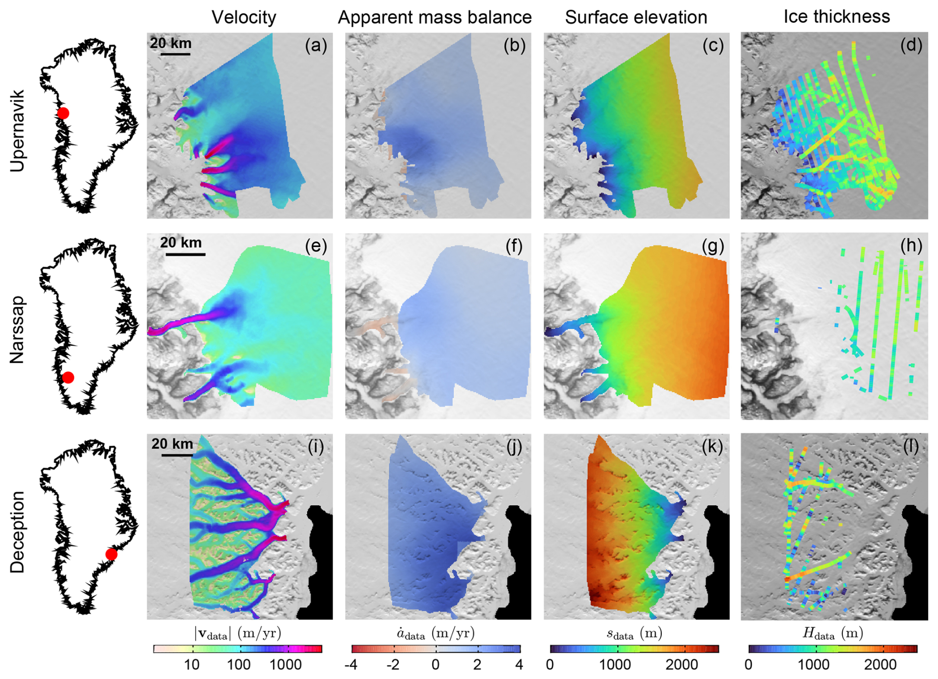
Figure 2 Training data for three regions in Greenland. Each row corresponds to the data for the (a–d) Upernavik, (e–h) Narssap, and (i–l) Deception regions from which we select data points for training each PINN. The first column on the left shows the location of these regions on the GrIS. The subsequent columns, from left to right, contain the following information for the whole region: (a, e, i) magnitude of the ice velocity from NASA MEaSUREs, $\left|{\mathit{v}}_{\text{data}}\right|$ in log₁₀ scale, (b, f, j) apparent mass balance calculated using surface mass balance from RACMO 2.3 and ICESat-2 derived ice thinning rates, ${\dot{a}}_{\text{data}}$, (c, g, k) surface elevation from GIMP, s_data, and (d, h, l) ice thickness H_data, obtained along ice-penetrating radar flight tracks.

2.4 Regions of Interest

We focus on three different regions of Greenland in order to test the PINN frameworks in different environments as shown in Figs. 2 and 3. We first focus on the region depicted in Fig. 2a–d in West Greenland, which includes Nunatakassaap Sermia and the three main branches of Upernavik Isstrøm, labelled in Fig. 3a. For simplicity we will refer to this region as the “Upernavik” region. The bed topography in this region is well constrained as there are relatively dense ice thickness measurements from ice-penetrating radar, as shown in Fig. 2d, making it appropriate for assessing the overall performance of the PINN. We then focus on a region in Southwest Greenland, where the ice velocities are slower, ice thickness measurements are limited, and the bed topography is not well known. This “Narssap” region, shown in Fig. 2e–h includes Narssap Sermia, Qamanaarsuup Sermia, and Akullersuup Sermia, labelled in Fig. 3b. Finally, we focus on the “Deception” region in Southeast Greenland, which has several fast-flowing, tributary ice streams, shown in Fig. 2i–l. The main outlet glaciers are Unnamed Deception Ø Central North, Unnamed Deception Ø Central South, Unnamed Uunartit Islands, and Kruuse Fjord, which are labelled in Fig. 3c. This region has sparse ice thickness measurements, a complex, alpine-like bed topography and slower ice velocities in between fast-flowing ice streams, making the mass-conserving approach of BedMachine difficult to implement (Morlighem et al., 2017).

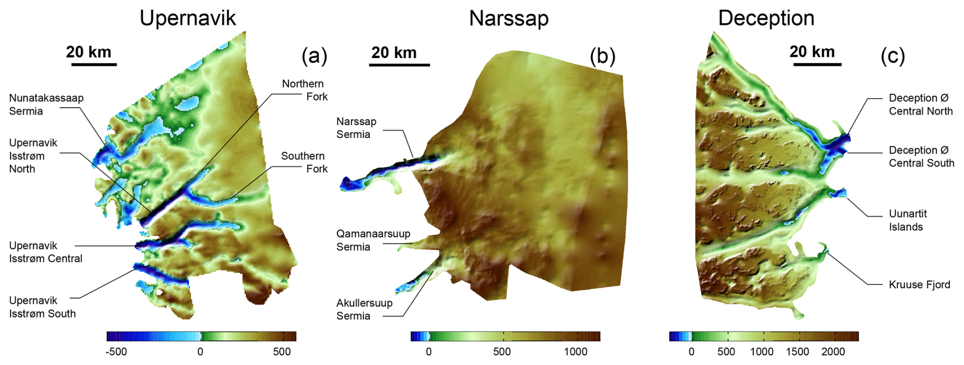
Figure 3 BedMachine Greenland (Version 6) bed topographies for (a) Upernavik, (b) Narssap, and (c) Deception regions, which we calculate using surface elevation from GIMP and BedMachine ice thickness. Each of the regions are annotated with the main outlet glaciers and fast-flowing ice streams.

2.5 Loss Function

Following the PINN architecture in Fig. 1, when a PINN constrained by two conservation laws is provided with input tensors $(\widehat{\mathit{x}},\widehat{\mathit{y}})$, it will predict tensors of the state variables of both mass balance and stress balance at the distinct locations selected for training (i.e., the data points), including $\widehat{\mathit{v}}=({\widehat{\mathit{v}}}_x,{\widehat{\mathit{v}}}_y{)}^{⊺}$ (predicted ice velocity), $\widehat{\dot{\mathit{a}}}$ (predicted apparent mass balance), $\widehat{\mathit{s}}$ (predicted surface elevation), $\widehat{\mathit{H}}$ (predicted ice thickness), and $\widehat{\mathit{C}}$ (predicted basal friction coefficient).

Let all N_(⋅) terms represent the number of data points associated with their corresponding subscripts (as defined in Sect. 2.2). We denote different N_(⋅) values for each variable because these data points are not necessarily in the same location as each other, which is standard practice when training PINNs (e.g., Cheng et al., 2024, 2025b). Then, supposing that $\Vert \widehat{\mathit{f}}{\Vert }^{\mathrm{2}}={\mathrm{\Sigma }}_{j=\mathrm{1}}^N(f_j{)}^{\mathrm{2}}$ for any tensor $\widehat{\mathit{f}}=(f_{\mathrm{1}},\mathrm{\dots },f_N{)}^{⊺}$, we define the following data loss terms:

$$\begin{array}{ll}{\displaystyle }{\mathcal{L}}_{\mathrm{v}}& {\displaystyle }={\displaystyle \frac{{\mathit{\gamma }}_{\mathrm{v}}}{N_{\mathrm{v}}}}\Vert {{\widehat{\mathit{v}}}_x}_{\text{data}}-{\widehat{\mathit{v}}}_x{\Vert }^{\mathrm{2}}+{\displaystyle \frac{{\mathit{\gamma }}_{\ln \mathrm{v}}}{N_{\mathrm{v}}}}{∥\ln {\displaystyle \frac{\left|{{\widehat{\mathit{v}}}_{\mathit{x}}}_{\text{data}}\right|+\mathit{\epsilon }}{\left|{\widehat{\mathit{v}}}_x\right|+\mathit{\epsilon }}}∥}^{\mathrm{2}}\\ \text{(7)}& {\displaystyle }& {\displaystyle }+{\displaystyle \frac{{\mathit{\gamma }}_{\mathrm{v}}}{N_{\mathrm{v}}}}\Vert {{\widehat{\mathit{v}}}_y}_{\text{data}}-{\widehat{\mathit{v}}}_y{\Vert }^{\mathrm{2}}+{\displaystyle \frac{{\mathit{\gamma }}_{\ln \mathrm{v}}}{N_{\mathrm{v}}}}{∥\ln {\displaystyle \frac{\left|{{\widehat{\mathit{v}}}_{\mathit{y}}}_{\text{data}}\right|+\mathit{\epsilon }}{\left|{\widehat{\mathit{v}}}_y\right|+\mathit{\epsilon }}}∥}^{\mathrm{2}},\text{(8)}& {\displaystyle }{\mathcal{L}}_{\dot{a}}& {\displaystyle }={\displaystyle \frac{{\mathit{\gamma }}_{\dot{a}}}{N_{\dot{a}}}}\Vert {\widehat{\dot{\mathit{a}}}}_{\text{data}}-\widehat{\dot{\mathit{a}}}{\Vert }^{\mathrm{2}},\text{(9)}& {\displaystyle }{\mathcal{L}}_s& {\displaystyle }={\displaystyle \frac{{\mathit{\gamma }}_s}{N_s}}\Vert {\widehat{\mathit{s}}}_{\text{data}}-\widehat{\mathit{s}}{\Vert }^{\mathrm{2}},\text{(10)}& {\displaystyle }{\mathcal{L}}_H& {\displaystyle }={\displaystyle \frac{{\mathit{\gamma }}_H}{N_H}}\Vert {\widehat{\mathit{H}}}_{\text{data}}-\widehat{\mathit{H}}{\Vert }^{\mathrm{2}},\end{array}$$

where the data loss terms ℒ_(⋅) correspond to the MSE with respect to their subscripts (as defined in Sect. 2.2). The velocity data loss term ℒ_v shown in Eq. (7) includes two additional logarithmic terms that allow the PINN to capture slower ice velocities. These logarithmic terms include a small number $\mathit{\epsilon }\sim {\mathrm{10}}^{-\mathrm{16}}$ to prevent taking the natural log of or dividing by zero. Given the framework depicted in Fig. 1, we note that the PINN is required to predict the basal friction coefficient in order to compute the stress balance residual, however we do not include a basal friction data loss term in the overall loss function since we do not have direct observations of the same.

For the physical loss terms, we randomly select N_φ collocation points $\mathit{\{}{\mathit{x}}_j{\mathit{\}}}_{j=\mathrm{1}}^{N_{\mathit{\phi }}}\in \mathrm{\Omega }$ to compute mass balance and stress balance shown in Eqs. (3) and (4) respectively. In particular, we denote tensors of the mass balance and stress balance residuals at these collocation points as ${\widehat{\mathit{\phi }}}_{\text{MB}}$ and ${\widehat{\mathit{\phi }}}_{\text{SB}}=({\widehat{\mathit{\phi }}}_{{\text{SB}}_x},{\widehat{\mathit{\phi }}}_{{\text{SB}}_y}{)}^{⊺}$ respectively. Then, we define the following physical loss terms:

$$\begin{array}{}\text{(11)}& {\displaystyle }{\mathcal{L}}_{{\mathit{\phi }}_{\text{MB}}}& {\displaystyle }={\displaystyle \frac{{\mathit{\gamma }}_{\text{MB}}}{N_{\mathit{\phi }}}}\Vert {\widehat{\mathit{\phi }}}_{\text{MB}}{\Vert }^{\mathrm{2}},\text{(12)}& {\displaystyle }{\mathcal{L}}_{{\mathit{\phi }}_{\text{SB}}}& {\displaystyle }={\displaystyle \frac{{\mathit{\gamma }}_{\text{SB}}}{N_{\mathit{\phi }}}}\Vert {\widehat{\mathit{\phi }}}_{{\text{SB}}_x}{\Vert }^{\mathrm{2}}+{\displaystyle \frac{{\mathit{\gamma }}_{\text{SB}}}{N_{\mathit{\phi }}}}\Vert {\widehat{\mathit{\phi }}}_{{\text{SB}}_y}{\Vert }^{\mathrm{2}}.\end{array}$$

where the ${\mathcal{L}}_{{\mathit{\phi }}_{(\cdot )}}$ terms correspond to the MSE of the PDE residuals with respect to their subscripts: MB (Mass Balance) and SB (Stress Balance).

Table 1 Typical values of variables, selected weighting terms for the loss function, and number of data points and collocation points chosen for all three regions

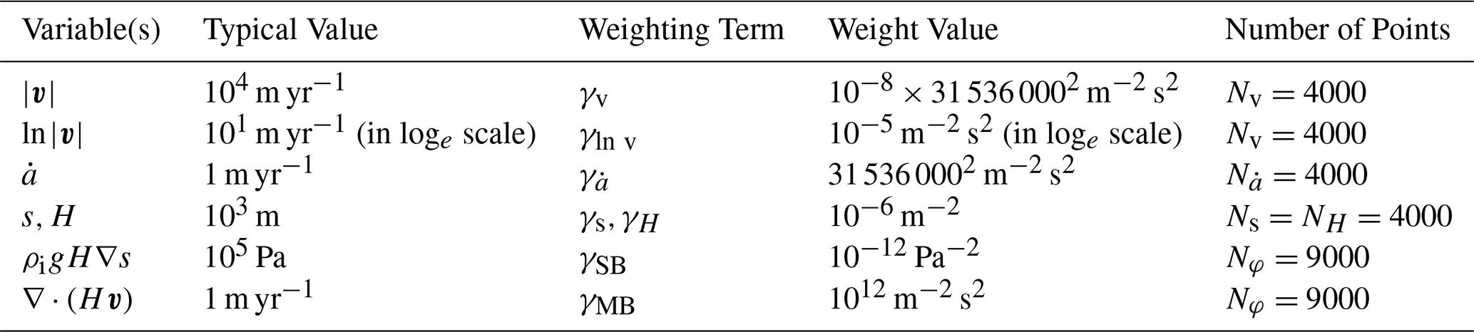
All the γ_(⋅) coefficients represent carefully selected scaling terms, or loss function weights, following a similar strategy to Cheng et al. (2024). All γ_(⋅) weights ensure that each of the loss terms contribute similarly to the overall loss within the SI unit system. Both the data loss and physical loss terms are scaled to roughly the same order of magnitude using the typical values of variables in ice sheet modeling applications, as shown in Table 1. While we are using the same weighting terms (from Table 1) for all of our regions, we acknowledge that there is scope for more flexibility in choosing these weighting terms as the PINN output variables will have different values for different regions of the GrIS. Indeed, the γ_(⋅) coefficients presented in this paper differ slightly from those provided by Cheng et al. (2024, 2025b). Table 1 provides further details on the typical values of these variables, the corresponding weights, and the number of data points and collocation points chosen for training.

2.6 Experiments

For each of the three experiments, described below, we train the same PINN multiple times to obtain a median prediction for each of the PINN output variables. This approach is necessary because the mixed inverse problem is ill-posed and the PINN training process is sensitive to randomness. More specifically, the initial state of the PINN (i.e., the initial neural network weights), the locations of collocation points, and the selection of data points are all determined randomly, implying that the final PINN predictions for each region may vary. As such, we train five PINNs for each experiment with different random seeds and retrieve the median prediction over a given region of interest. We find an ensemble of five PINNs for each region to be suitable given the computational cost of training a single PINN (further details on compute time can be found in the Results section). Moreover, since we have chosen a high number of iterations for training each PINN, we expect the predictions to generally converge. It should be noted that we choose to retrieve the median prediction rather than the mean prediction, which is less robust to biases.

2.6.1 Mass Balance

The goal of this experiment is to assess how well PINNs perform in regions where the mass-conserving approach of BedMachine is challenging to implement, such as regions where the ice is moving too slowly and the inversion is not well constrained. Hence, we train PINNs constrained with only the mass balance residual shown in Eq. (3) for Deception, which is a complex region with sparse measurements and slow-moving ice in between fast-flowing ice streams. Henceforth, we will refer to this PINN as “PINN (MB)” (or PINN constrained with Mass Balance only).

The architecture of the PINN (MB) differs slightly from the architecture illustrated in Fig. 1. When provided with input tensors $(\widehat{\mathit{x}},\widehat{\mathit{y}})$, PINN (MB) will predict output tensors of the state variables of the conservation of mass. Therefore, we construct the following loss function, denoted by ℒ_MB, to inform predictions:

$$\begin{array}{}\text{(13)}& {\mathcal{L}}_{\text{MB}}={\mathcal{L}}_{\mathrm{v}}+{\mathcal{L}}_{\dot{a}}+{\mathcal{L}}_H+{\mathcal{L}}_{{\mathit{\phi }}_{\text{MB}}}\end{array}$$

where all the loss terms ℒ_(⋅) are defined in Eqs. (7), (8), (10), and (11). We retain all N_(⋅) and γ_(⋅) values from Table 1 for PINN (MB). The PINN (MB) is constrained by ice thickness data along the ice-penetrating radar flight tracks shown in Fig. 2l.

2.6.2 Stress Balance

Recent work by Cheng et al. (2024) demonstrated the application of PINNs constrained with only the conservation of momentum to the fast-flowing region of Helheim Glacier. However, it remains unclear whether this PINN framework would be as effective as BedMachine in regions with more complex topography, sparse measurements, and slower ice velocities. To explore this further, we implement a PINN constrained with only the stress balance residual shown in Eq. (4) for the Deception region. We refer to this PINN as “PINN (SB)” (or PINN constrained with Stress Balance only).

Similar to PINN (MB), the architecture of PINN (SB) also differs slightly from the architecture illustrated in Fig. 1. When provided with input tensors $(\widehat{\mathit{x}},\widehat{\mathit{y}})$, PINN (SB) will predict output tensors of the state variables of the conservation of momentum. Therefore, we construct the following loss function, denoted by ℒ_SB, to inform predictions:

$$\begin{array}{}\text{(14)}& {\mathcal{L}}_{\text{SB}}={\mathcal{L}}_{\mathrm{v}}+{\mathcal{L}}_s+{\mathcal{L}}_H+{\mathcal{L}}_{{\mathit{\phi }}_{\text{SB}}}\end{array}$$

where all the loss terms ℒ_(⋅) are defined in Eqs. (7), (9), (10), and (12). We retain all N_(⋅) and γ_(⋅) values from Table 1 for PINN (SB). Cheng et al. (2024) included additional loss terms describing boundary conditions on the calving front of Helheim Glacier, however since we are only solving the inverse problem (and not the forward problem), we do not include any loss terms for calving. The PINN (SB) is constrained by randomly selected ice velocity data both within the domain and along the boundaries of the region of interest.

2.6.3 Coupling Mass Balance and Stress Balance

The results of BedMachine Greenland and Cheng et al. (2024) suggest that that informing PINNs with mass conservation or momentum conservation alone may not be sufficient to retrieve accurate predictions of ice thickness in slower-moving regions with sparse ice thickness measurements and complex topographies. While using the classical adjoint method to solve for the ice thickness and basal sliding coefficient is technically difficult, this PINN framework (Fig. 1) allows us to easily and flexibly introduce multiple PDE constraints within our loss function. Hence, we implement a PINN constrained with both mass balance, Eq. (3), and stress balance, Eq. (4), for the regions of interest, described above. These PDEs are coupled within the PINN framework as predicted ice thickness values that satisfy the mass balance residual are directly substituted into the stress balance residuals, and vice versa. Henceforth, we refer to the PINN in this experiment as “PINN (MB + SB)” (or PINN constrained with both Mass Balance and Stress Balance).

As shown in Fig. 1, when this PINN (MB + SB) is provided with input tensors $(\widehat{\mathit{x}},\widehat{\mathit{y}})$, it will predict output tensors of the state variables of both the conservation of mass and the conservation of momentum. Therefore, we construct the following loss function, denoted by ℒ, to inform predictions:

$$\begin{array}{}\text{(15)}& \mathcal{L}={\mathcal{L}}_{\mathrm{v}}+{\mathcal{L}}_{\dot{a}}+{\mathcal{L}}_{\mathrm{s}}+{\mathcal{L}}_H+{\mathcal{L}}_{{\mathit{\phi }}_{\text{MB}}}+{\mathcal{L}}_{{\mathit{\phi }}_{\text{SB}}}\end{array}$$

where the loss terms ℒ_(⋅) are defined in Eqs. (7), (8), (9), (10), (11), and (12). We retain all N_(⋅) and γ_(⋅) values from Table 1 for this PINN (MB + SB). Similar to previous experiments, constraints for this mixed inverse problem are provided by ice-thickness and velocity data.

3 Results

Depending on the configuration of PDE constraints, each PINN took approximately 3–17 h to train using one NVIDIA A100 PCIE 40GB GPU (Texas Advanced Computing Center, 2026). We train five PINNs for each experiment with different random seeds to deal with the random nature of the PINN training process. Unless otherwise stated, all reported results refer to the median prediction of five PINNs.

3.1 Effect of Different Physical Constraints

To assess the effect of different physical constraints, we present PINN (MB), PINN (SB), and PINN (MB + SB) predictions of the bed topography for Deception. For each experiment, we use predictions of the ice thickness, H, and the surface elevation from GIMP, s_data, to calculate the predicted bed topography, $b=s_{\text{data}}-H$ for the whole region, as depicted in Fig. 4a–c. The differences between predicted bed topographies and BedMachine Greenland (Version 6) are depicted in Fig. 4d–f, with the areas in which BedMachine applies a mass-conserving approach outlined in black; henceforth we will refer to these outlined areas as Ω_mc.

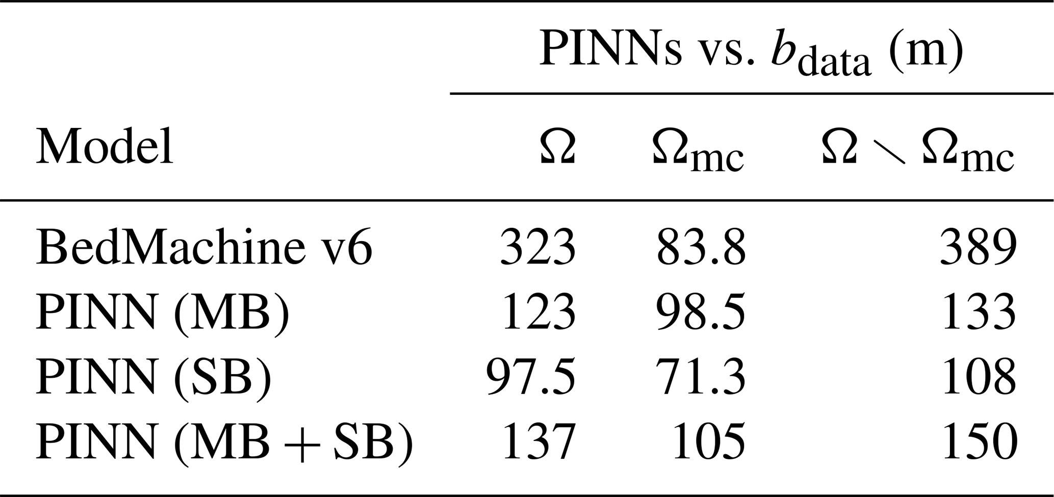
Table 2 Bed topography RMSEs for Deception along ice-penetrating radar flight tracks, for different physical constraints.

To assess the accuracy of the predicted bed topographies, we compare predictions along ice-penetrating radar flight tracks to “ground-truth data” obtained along the same flight tracks. We compute these reference bed elevations by taking the difference between observed surface elevation along the flight tracks and ice thickness measurements, $b_{\text{data}}=s_{\text{data}}-H_{\text{data}}$. The root mean squared errors (RMSEs) between the inferred and reference bed topographies are compiled into Table 2.

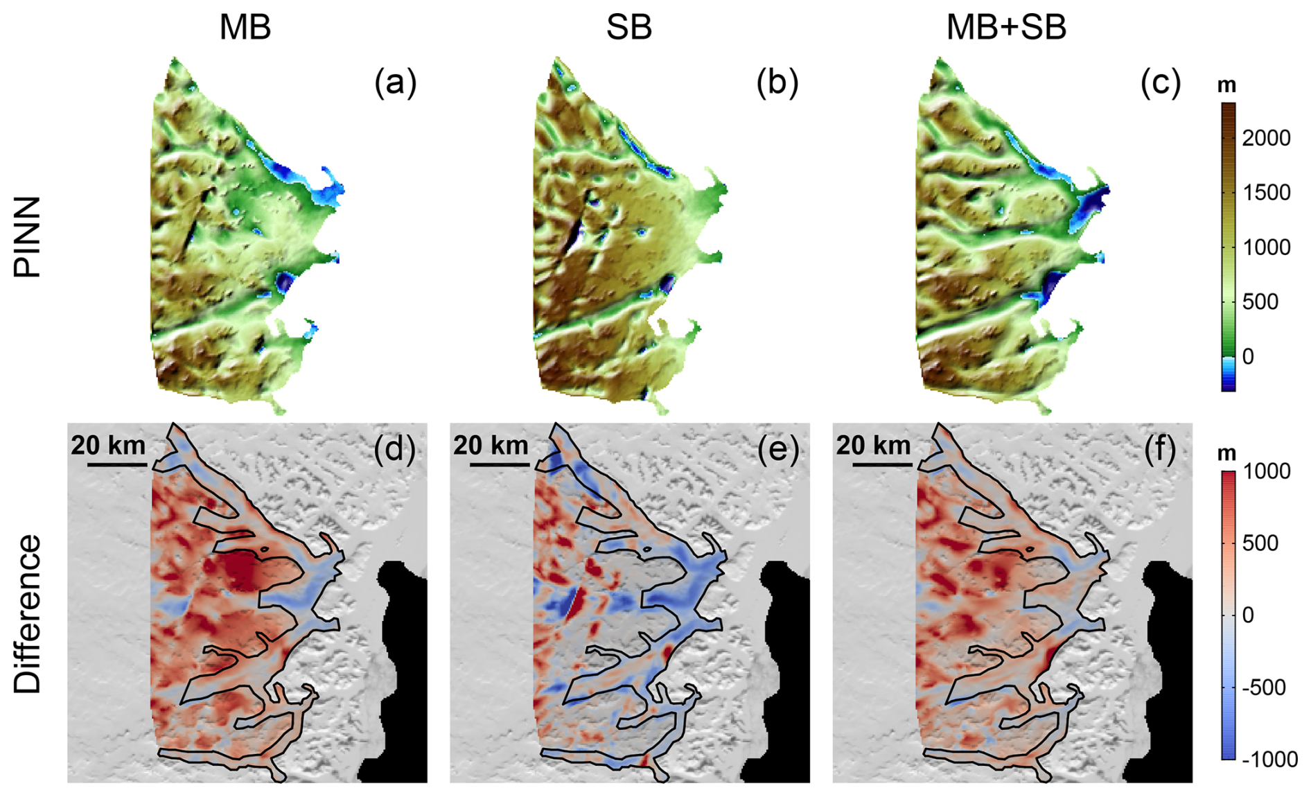
Figure 4 Inferred bed topography maps for Deception to demonstrate the effect of different physical constraints. The depicted maps are for (a, d) PINN (MB), (b, e) PINN (SB), and (c, f) PINN (MB + SB). From top to bottom, (a)–(c) show the PINN inferred bed topography maps, and (d)–(f) show the difference between BedMachine and PINN bed topography maps, b_BedMachine−b (m). On these difference maps, we outline the areas in which BedMachine uses a mass-conserving approach, Ω_mc (i.e., the black outline).

The BedMachine and PINN (MB) topographies are quite different as shown in Fig. 4d, especially outside of Ω_mc where differences exceed 800 m in some areas. PINN (MB) predictions align more closely with the ground-truth bed topography, as indicated by the relatively low RMSE of 123 m compared to the BedMachine RMSE of 323 m (see Table 2). However, we also notice that PINN (MB) predicts bed features that are highly correlated to the ice-penetrating radar flight tracks in Fig. 2l. Within Ω_mc, the average difference between BedMachine and PINN (MB) is significantly reduced, with differences of approximately 300 m. Yet, PINN (MB) tends to predict thinner ice than ice-penetrating radar measurements suggest. As a result, PINN (MB) does not capture the depth of the troughs beneath Deception Ø Central North, Deception Ø Central South and Uunartit Islands that are better resolved by BedMachine. Indeed, the PINN (MB) RMSE within Ω_mc of 98.5 m is higher than the BedMachine RMSE of 83.8 m (see Table 2).

For PINN (SB), we notice that the predicted bed topography for Deception is relatively similar to BedMachine outside Ω_mc, as shown by the grey areas on the difference map in Fig. 4e. More quantitatively, the PINN (SB) RMSE of 108 m outside Ω_mc is significantly lower than the BedMachine RMSE of 389 m outside Ω_mc (see Table 2). We observe that PINN (SB) predicts isolated crater-like depressions along ice-penetrating radar flight tracks, shown in Fig. 4b. Within Ω_mc, the difference between BedMachine and PINN (SB) is more pronounced, with differences of approximately 600 m. Interestingly, though the PINN (SB) RMSE of 71.3 m is slightly lower than the BedMachine RMSE of 83.8 m within Ω_mc, PINN (SB) predicts thinner ice than ice-penetrating radar measurements suggest and fails to capture the troughs beneath Deception Ø Central North, Deception Ø Central South and Uunartit Islands that are well captured in BedMachine.

Lastly, we observe that the Bedmachine and PINN (MB + SB) bed topographies are significantly different. However, unlike PINN (MB) and PINN (SB), which predict isolated bed features that coincide with radar flight tracks, the PINN (MB + SB) bed topography for Deception consists of an intricate network of troughs that are not well captured in BedMachine. PINN (MB + SB) appears to connect and interpolate bed features between radar flight tracks, where we have direct observations. Though we observe differences of over 600 m outside Ω_mc, as shown in Fig. 4f, the PINN (MB + SB) RMSE of 137 m is lower than that of BedMachine (see Table 2). Within Ω_mc, PINN (MB + SB) does capture the troughs beneath Deception Ø Central North, Deception Ø Central South and Uunartit Islands. However, the predicted ice thickness is slightly thinner than suggested by radar-derived measurements and BedMachine. As a final note, we determine that PINN (MB + SB) produces accurate predictions through a separate validation study and refer the reader to Appendix B.

3.2 Predictions for Regions of Interest

We present the applications of PINN (MB + SB) to the three regions of interest: Upernavik, Narssap, and Deception. Further detail on our results, including the predicted basal friction coefficients, can be found in Appendix A.

3.2.1 Predictions of the Bed Topography

We calculate the predicted bed topography, b, for each region as shown in Fig. 5a–c and compare these bed topographies to the BedMachine bed topographies shown in Fig. 3. We show the difference between the BedMachine and PINN bed topographies in Fig. 5d–f, annotated with Ω_mc. To assess the PINN results, we compare predictions along ice-penetrating radar flight tracks to ground-truth bed topography data, b_data, and compile the RMSEs into in Table 3. We also estimate the uncertainty in PINN predictions of ice thickness by assessing the spread in ice thickness projections of the PINN (MB + SB) ensemble (Fig. 6).

Table 3 Bed topography RMSEs for Upernavik, Narssap, and Deception along ice-penetrating radar flight tracks. The table contains RMSEs between PINN-predicted bed topographies and ground-truth ice-penetrating radar observations, b_data (m), both within and outside Ω_mc. For comparison, we also include RMSEs between BedMachine (Version 6) bed topographies and ground-truth ice-penetrating radar observations within and outside Ω_mc.

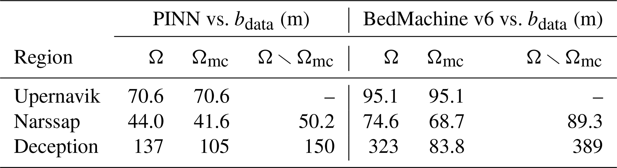
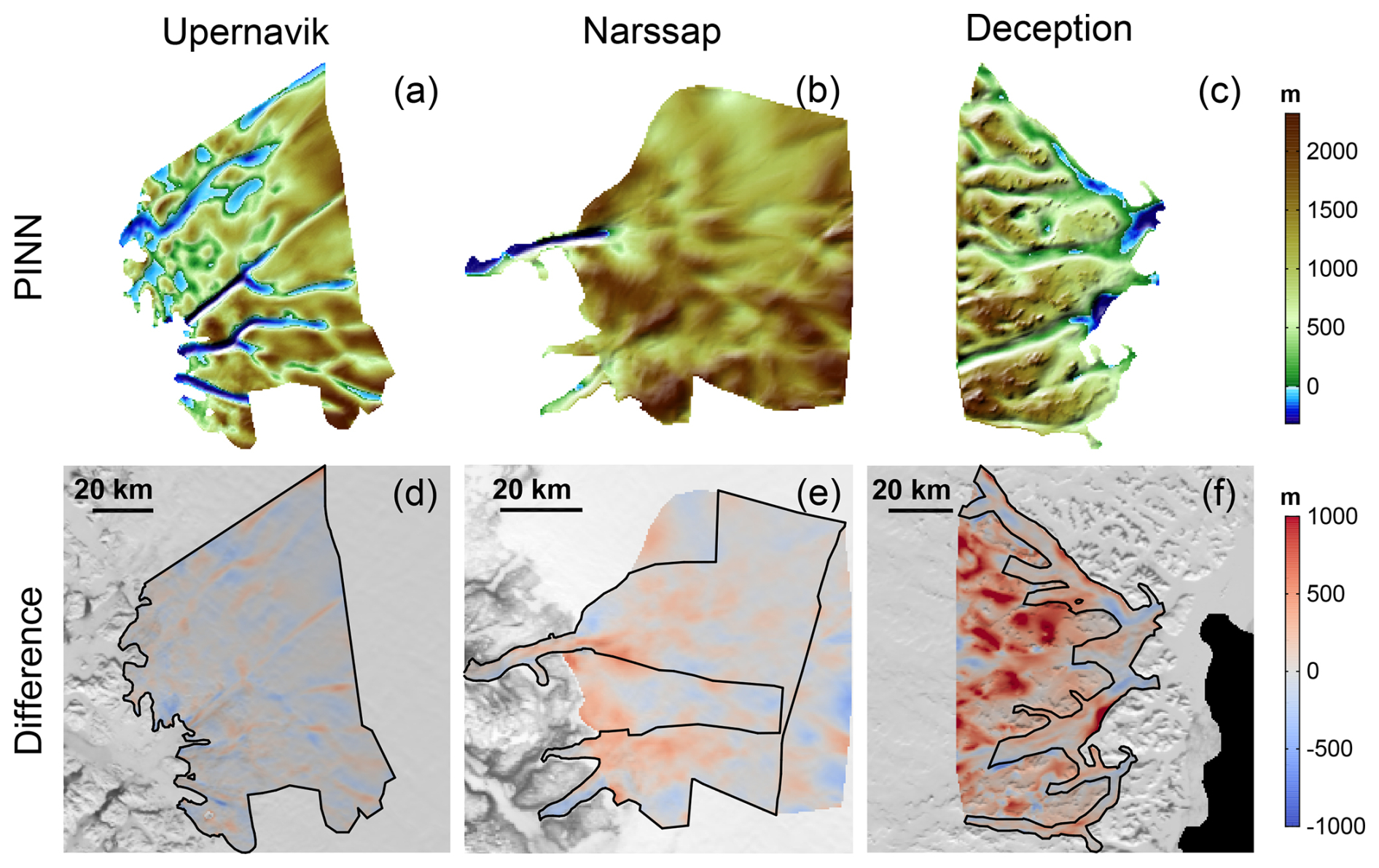
Figure 5 PINN (MB + SB) bed topography and difference maps for (a, d) Upernavik, (b, e) Narssap, and (c, f) Deception. (a)–(c) depict the PINN (MB + SB) predicted bed topography maps, and (d)–(f) depict the difference between BedMachine and the PINN bed topography maps, b_BedMachine−b (m). These difference maps are also annotated with an outline of Ω_mc for each region (in black).

For Upernavik, the BedMachine and PINN bed topographies, shown in Figs. 3a and 5a respectively, are broadly similar with an average difference of less than 100 m for the whole region. The PINN RMSE of 70.6 m (compared to ground-truth bed topography data) is lower than the BedMachine RMSE of 95.1 m (see Table 3), and indeed, we observe a few noticeable differences between these bed topographies. Going from north to south, the PINN predicts a continuous trough beneath Nunatakassaap Sermia, while BedMachine does not. Second, the PINN indicates that the trough beneath the northern fork of Upernavik Isstrøm North extends further inland than BedMachine suggests. Lastly, the PINN predicts a “disconnected” trough beneath the southern fork of Upernavik Isstrøm North, while BedMachine suggests that this trough is continuous.

Comparing the PINN bed topographies for Narssap in Fig. 5b and BedMachine in Fig. 3b, we observe that the PINN infers glacial valleys in the bed, especially outside Ω_mc. These features satisfy ground-truth bed topography data as indicated by the relatively low RMSE of 50.2 m compared to the BedMachine RMSE of 89.3 m (see Table 3). Within Ω_mc, the PINN predicts troughs beneath Narssap Sermia and Akullersuup Sermia that are shallower than those in both BedMachine and ground-truth data by approximately 200 m.

The BedMachine and PINN bed topographies for Deception, shown in Figs. 3c and 5c are significantly different. The PINN predicts an intricate network of troughs that coincide with the fast-flowing ice streams and are not well captured in BedMachine. These differences are especially evident outside Ω_mc in Fig. 5f, with the PINN showing that the bed topography is deeper than that of BedMachine by over 600 m. Despite this rather large difference with respect to BedMachine, these PINN inferred bed features satisfy ground-truth bed topography data, as indicated by the relatively low RMSE of 150 m compared to the BedMachine RMSE of 389 m outside Ω_mc (see Table 3). Within Ω_mc, the PINN predicts troughs beneath Deception Ø Central South and Uunartit Islands that are shallower than that of both BedMachine and ground-truth data by approximately 250 m.

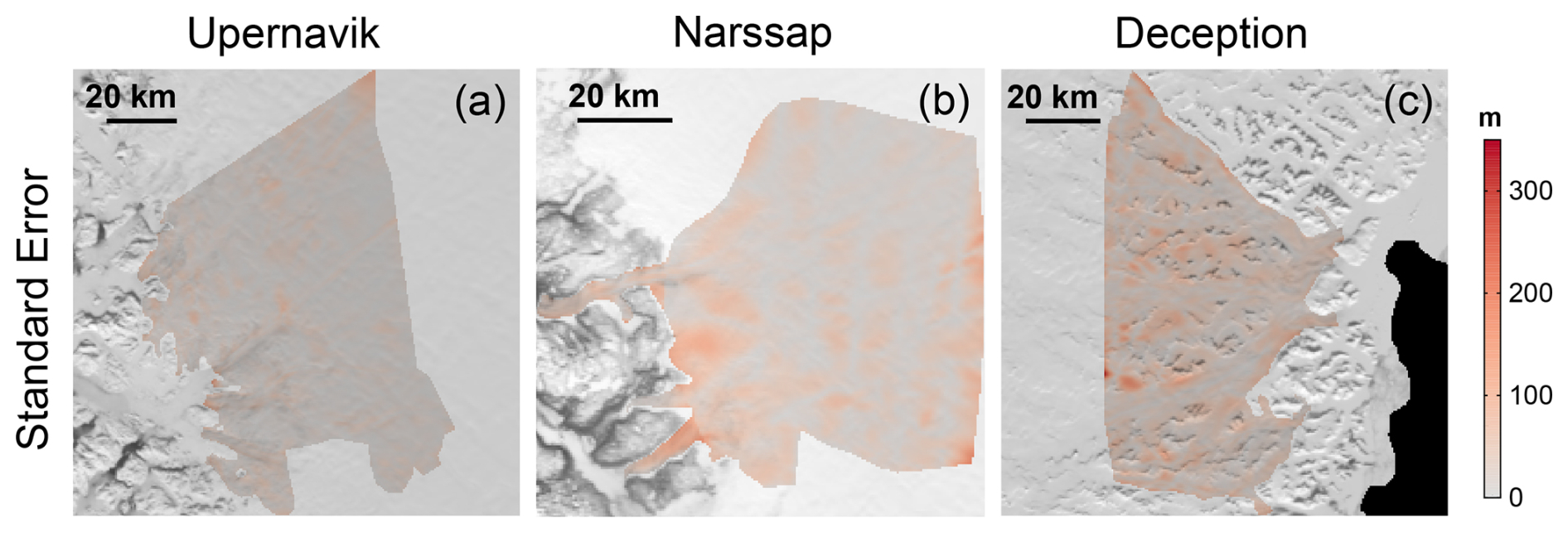
Figure 6 Standard error in PINN (MB + SB) ice thickness predictions for (a) Upernavik, (b) Narssap, and (c) Deception. Note that we calculate the standard error by dividing the standard deviation in ice thickness predictions by the square root of the sample size n=5 (i.e., number of PINNs in the ensemble).

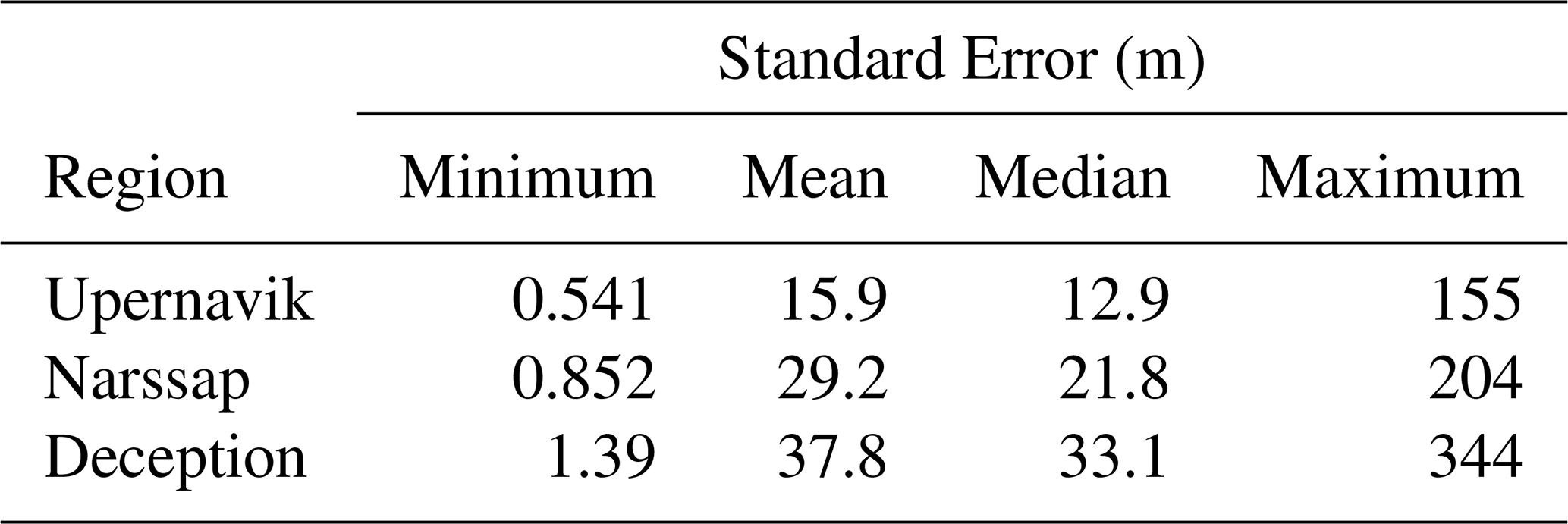
Since we train an ensemble of PINNs and retrieve the median prediction, in reality we have a range of ice thickness predictions for each (x,y) location. To estimate the uncertainty due to the initial state of the PINN, we assess the spread in PINN predictions within the ensemble for each region by calculating the standard error of the ice thickness predictions, shown in Fig. 6. The mean and median standard errors in ice thickness predictions across all regions are ≲40 m. For the Upernavik region, we generally observe lower standard error values with a maximum of 155 m. The standard errors for Narssap and Deception are slightly higher, with maximum standard error values of 204 and 344 m respectively. These results are compiled into Table 4.

Table 4 Standard Error in ice thickness predictions within PINN (MB + SB) ensemble for Upernavik, Narssap, and Deception. For each region of interest, we determine the minimum and maximum standard error in ice thickness predictions. Additionally, we also calculate the mean and median standard error values to provide more insight into the distribution of these standard errors.

3.2.2 Predictions of Observable Ice Sheet Features

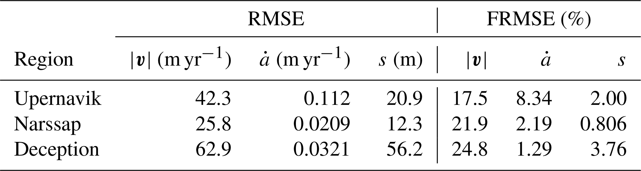
We present PINN predictions of the observable ice sheet features (including v, $\dot{a}$, and s) for all three regions of interest. It is important that the PINN accurately predicts these observable features as these predictions are used to compute the PDE residuals in the loss function, and therefore the bed prediction. Table 5 describes the RMSEs and fractional root mean squared errors (FRMSEs) between PINN predictions and the training data for these observable features. Note that we calculate the FRMSE (as a percentage) using Eq. (16):

$$\begin{array}{}\text{(16)}& \begin{array}{rl}\text{FRMSE (\%)}& ={\displaystyle \frac{\sqrt{{\displaystyle \frac{\mathrm{1}}{N}}{\sum }_{i=\mathrm{1}}^N(y_{{\text{data}}_{\mathrm{i}}}-y_{\mathrm{i}}{)}^{\mathrm{2}}}}{{\displaystyle \frac{\mathrm{1}}{N}}{\sum }_{i=\mathrm{1}}^N\left|y_{{\text{data}}_{\mathrm{i}}}\right|}}\times \mathrm{100}\mathit{\%}\\ & ={\displaystyle \frac{\text{RMSE}}{{\displaystyle \frac{\mathrm{1}}{N}}{\sum }_{i=\mathrm{1}}^N\left|y_{{\text{data}}_{\mathrm{i}}}\right|}}\times \mathrm{100}\mathit{\%}\end{array}\end{array}$$

The PINNs are generally able to capture the ice velocities, though predictions have larger differences of over 100 m yr⁻¹ along fast-flowing ice streams, as shown in Fig. A1. Upernavik and Narssap velocity predictions have lower RMSEs of 42.3 and 25.8 m yr⁻¹ respectively, while the Deception velocity prediction has a higher RMSE of 62.9 m yr⁻¹, which is to be expected since Deception has faster-flowing glaciers. Interestingly, even though we see differences in the RMSEs of velocity predictions, the FRMSEs are all close to ∼20 %. Among all the observable features, the PINNs best capture the apparent mass balance within FRMSEs of 10 % for each region (shown in Table 5), though we notice minor differences along the margins, as shown in Fig. A2. The Narssap and Deception apparent mass balance predictions have lower RMSEs of 0.0209 and 0.0321 m yr⁻¹ respectively, while the RMSE of the apparent mass balance for Upernavik is an order of magnitude higher at 0.112 m yr⁻¹. The PINNs also generally capture the surface elevation for each region within FRMSEs of 5 %, though these predictions are smoother, implying that they are lower frequency approximations of the observed surface elevation from GIMP, as shown in Fig. A3. In other words, the PINNs do not resolve fine-scale (≲500 m) details in the surface elevation. The surface elevation predictions for Upernavik and Narssap have lower RMSEs of 20.9 and 12.3 m respectively, while the prediction for Deception, which has a complex topography, has an RMSE of 56.2 m. Further details on the predictions of the observable ice sheet features can be found in Appendix A.

Table 5 RMSEs and FRMSEs between PINN predictions (of the other variables in the PDEs) and the training data for each region.

4 Discussion

We first discuss the effect of informing PINNs with different physical constraints for the Deception region. After determining the most effective physical constraints for inferring the bed topography, we discuss PINN results for the three regions of interest. While the focus of this paper is on PINN predictions of the ice thickness, and subsequently the bed topography, a brief discussion of the PINN predictions for the second unknown, the basal friction, can be found in Appendix A. A further comparison of the PINN predicted bed topography to another bed topography product generated using a quantile regression forest approach (Palmer et al., 2025) can be found in Appendix D.

4.1 Determination of Physical Constraints

From the results presented in Fig. 4, we observe that all three PINNs (i.e., MB, SB, and MB + SB) predict significantly different bed topographies than that of BedMachine for the Deception region, especially outside Ω_mc. All three PINNs satisfy ground-truth bed topography data better than BedMachine outside Ω_mc, as indicated by the RMSEs in Table 2. However, PINN (MB) and PINN (SB) predict isolated, crater-like features along radar flight tracks as shown in Fig. 4a, b. Given the presence of fast-flowing, tributary ice streams in this region, these crater-like bed features are unrealistic. We expect that PINN (MB) and PINN (SB) are fitting the training data too closely and not interpolating or “connecting” inferred bed features. In other words, PINN (MB) and PINN (SB) are overfitting the training data, resulting in artificially lower RMSEs than that of BedMachine outside Ω_mc. PINN (MB + SB), however, predicts several troughs that coincide with the fast-flowing ice streams and satisfy ground-truth bed topography data outside of Ω_mc. Therefore we observe that PINN (MB + SB) successfully connects inferred bed features, leading to a far more realistic bed topography map for Deception. The PINN (MB + SB) RMSE of 150 m outside Ω_mc is slightly higher than the PINN (MB) and PINN (SB) RMSEs of 133 and 108 m respectively. This modest increase in the RMSE is expected, as PINN (MB + SB) uses multiple physical constraints, introducing additional regularization terms in its loss function. As a result, the slightly higher RMSE suggests that PINN (MB + SB) is learning a more generalized solution for the whole Deception region rather than overfitting the training data.

Within Ω_mc, the difference between BedMachine and PINN (SB) in Fig. 4e is more pronounced. Yet, interestingly, the PINN (SB) RMSE of 71.3 m is slightly lower than the BedMachine RMSE of 83.8 m within Ω_mc (see Table 2). The differences of over 500 m in Fig. 4(e) could be explained by the different physical constraints imposed within Ω_mc (i.e., PINN (SB) imposes stress balance while BedMachine imposes mass balance), though a more likely explanation for the PINN (SB) RMSE being low is due to overfitting. On the other hand, the reduced difference within Ω_mc for PINN (MB) and PINN (MB + SB) confirms that these PINNs are indeed using mass conservation to inform predictions. Yet, both PINN (MB) and PINN (MB + SB) predict thinner ice than that suggested by BedMachine and ice thickness measurements, failing to capture the full depth of the troughs beneath Deception Ø Central North, Deception Ø Central South, and Uunartit Islands. Indeed, the PINN (MB) and PINN (MB + SB) RMSEs of 98.5 and 105 m respectively is higher than the BedMachine RMSE even though the physical constraints imposed for all three are the same. We attribute this difference to the fact that BedMachine is exposed to all the available ice thickness, ice velocity, and apparent mass balance data, whereas the PINN is only exposed to a small subset of the ice thickness training data. Furthermore, BedMachine numerically solves for the ice thickness using the conservation of mass with the ground-truth ice velocity and apparent mass balance data directly. The PINN, on the other hand, makes predictions of the observable ice sheet features that are then used within the mass balance residual (in the loss function), thus not using the velocity and apparent mass balance data directly. The PINN predictions of these observable ice sheet features ($\mathit{v},\dot{a},s$) are not exactly equal to the ground-truth data, as shown by the differences in predicted and ground-truth ice velocities in Fig. A1, likely introducing numerical errors in the computation of the mass balance residual. These arguments imply that BedMachine imposes mass conservation more “strongly” within Ω_mc, while the PINNs impose the physical constraints more “weakly”. This may explain why BedMachine is able to resolve the full depth of the troughs beneath Deception Ø Central North, Deception Ø Central South, and Uunartit Islands within Ω_mc better than the PINNs.

To summarize, our results indicate that constraining the PINN with mass balance alone and stress balance alone is not sufficient for predicting realistic bed topography in complex regions, like Deception. Both PINN (MB) and PINN (SB) are prone to overfitting, especially outside Ω_mc. We determine that PINN (MB + SB) is most effective for inferring the bed topography as multiple physical constraints help mitigate overfitting, allowing for a more generalized prediction of the bed topography. It should be noted here that solving such a problem (i.e., coupling mass balance and stress balance) using the classical adjoint method, while theoretically possible, is technically difficult. While previous work has derived the classical adjoint using a first-order approximation of the Stokes equations and depth-integrated conservation of mass to simultaneously infer basal sliding and ice thickness (e.g., Perego et al., 2014), this problem is considerably more involved and, in practice, typically may necessitate automatic differentiation. The proposed PINN (MB + SB) framework provides a straightforward and flexible way to combine multiple physical constraints, thus exceeding their individual limitations while also fitting the training data, allowing for more realistic predictions.

4.2 Applications to Regions of Interest

We examine the predicted bed topography for Upernavik, shown in Fig. 5a. The difference map shown in Fig. 5d reveals that BedMachine and the PINN have broadly similar bed topography maps because they conserve the physical laws for the entire Upernavik region. The PINN is successful at “connecting” and extrapolating ice thickness measurements, revealing a realistically-looking, continuous trough beneath Nunatakassaap Sermia and an extended trough beneath the northern fork of Upernavik Isstrøm North, both of which are not captured in BedMachine. Given that the PINN RMSE of 70.6 m is lower than that of BedMachine, we expect that these new bed features satisfy ground-truth bed topography data and are realistic. Yet, in some cases where the PINN has no data points to further constrain it's predictions, it may not capture important bed features. For instance, the PINN does not infer a continuous trough beneath the southern fork of Upernavik Isstrøm North where there are no ice-penetrating radar measurements (see the ice thickness measurements along flight tracks in Fig. 2d). This means that the PINN would need to rely completely on the mass balance and stress balance residuals to infer the ice thickness, and subsequently the trough beneath. When we have no data points within Ω_mc to constrain predictions, we expect that BedMachine will produce more realistic results as it imposes mass conservation more “strongly” within Ω_mc, while the PINN enforces mass conservation and momentum conservation “weakly” (as discussed in Sect. 4.1). This may explain why the PINN did not successfully capture a continuous trough beneath the southern fork of Upernavik Isstrøm North, where the PINN has no data points to further constrain its predictions of ice thickness.

For Narssap, we note that Ω_mc generally encompasses the region with ice velocities that are ∼100 m yr⁻¹ or greater (see Fig. 2e). The PINN suggests glacial valleys outside Ω_mc which are not captured in BedMachine and satisfy ground-truth ice-penetrating radar measurements (see RMSEs in Table 3). We find these bed features to be realistic as they coincide directly with faster-flowing sectors, where velocities are approximately 50–100 m yr⁻¹. Within Ω_mc, we find that the PINN RMSE is lower than the BedMachine RMSE, implying that the PINN is satisfying ground-truth measurements better than BedMachine. However, in the fast-flowing region, we note that the PINN predicts thinner ice than that shown in Figs. 2h and 3b beneath Narssap Sermia and Akullersuup Sermia, implying that it is not able to recover the depth of the trough beneath these outlet glaciers. As mentioned above, PINN predictions of the ice velocity have larger uncertainties for the fast-flowing regions, such as Narssap Sermia and Akullersuup Sermia, which likely affects the computation of the PDE residuals. The PINN predictions of the surface elevation are smooth, which could also contribute to uncertainty in the PDE residuals, but since the PINN RMSE of 12.3 m for the surface elevation is relatively small we expect that most of the uncertainty in the PDE residuals is due to the velocity predictions. Furthermore, we observe that Narssap is a region with sparse ice thickness measurements and that the PINN conserves mass and momentum more “weakly” than BedMachine which “strongly” imposes mass balance along these fast-flowing regions within Ω_mc, likely explaining why BedMachine is able to recover the depth of the trough beneath Narssap Sermia and Akullersuup Sermia, while the PINN is not as successful.

The Deception region is known to have a complex topography and we note that Ω_mc is quite small, covering only the margins of the region as indicated by the black outline in Fig. 5f, where the ice velocities are approximately 1000 m yr⁻¹ or greater. The PINN unveils an intricate network of troughs outside Ω_mc that satisfy ground-truth bed topography measurements with lower RMSEs than BedMachine (see Table 3). Similar to Narssap, we find that these inferred features coincide with fast-flowing ice streams outside Ω_mc. Yet, also similar to Narssap, the PINN predicts thinner ice than shown in Fig. 2i within Ω_mc and consequently does not quite capture the full depth of the trough beneath Deception Ø Central North, Deception Ø Central South and Uunartit Islands. Similar to previous cases, this difference is explained by the fact that Ω_mc encompasses the region with fast-flowing ice where the PINN predictions of the ice velocity are more uncertain (see Fig. A1f) and by the fact that the PINN imposes the conservation laws weakly compared to BedMachine.

The uncertainty or spread in PINN predictions in the ensemble is generally ≲40 m across all regions (as indicated by the mean and median standard error values in Table 4). This implies that the uncertainty in predictions due to randomness and differences in the initial states of each PINN within the ensemble is generally lower than the overall bed topography RMSE values of Table 3. As expected, the spread in ice thickness predictions is lower for the Upernavik region than the other two regions as Upernavik has denser ice thickness measurements, meaning that the ice thickness predictions are more constrained. For Narssap and Deception, we notice that the standard errors are higher, especially between ice-penetrating radar flight tracks where predictions are more difficult to constrain. Yet, it is clear from the low mean and median standard error values (Table 4) as well as the standard error maps in Fig. 4 for all three regions that the PINNs generally agree with each other and converge to similar solutions for the ice thickness.

4.3 Limitations and Next Steps

Regarding the differences in the PINN predictions of the state variables (i.e., $\mathit{v},\dot{a},s$), we expect that these can be explained by the PINN model resolution. In other words, these differences are likely the result of too few data points provided to the PINN during the training process. We observe that the PINN captures observable features with gradual, smoother transitions (or gradients) better than those with sharper transitions. For instance, the PINN accurately predicts the apparent mass balance, which changes far more gradually across the regions of interest, but struggles to capture faster flowing ice velocities that have sharper gradients. As a result, increasing the number of data points and providing the PINN with more spatial information regarding these observable features will help limit the differences in all state variable predictions. That being said, it should be noted that increasing the number of data points and collocation points would lead to an increase in computational cost. Furthermore, we expect that we will not be able to limit small differences altogether with our current framework due to the nature of the PINN architecture itself (Krishnapriyan et al., 2021); the de-noising nature of the PINN lends itself to smoother, lower-frequency predictions. To address this limitation, we may have to employ a multi-stage training scheme (Wang and Lai, 2024).

Another main limitation of the PINN (MB + SB) framework is that it does not account for some of the physics, such as vertical shear and internal deformation. We acknowledge that vertical shear should not be neglected in areas of slower-moving ice, which is not accounted for in our current stress balance residual (i.e., the Shallow-Shelf Approximation). In making the assumption that the surface velocities are similar to depth-averaged velocities, we actually have slightly “inflated” depth-averaged velocities. Therefore, in order for the stress balance residual to be satisfied, the PINN would have to predict thinner ice to maintain the same ice flux. As our next steps will likely involve applying this method to interior regions of the Greenland Ice Sheet where BedMachine does not use a mass-conserving approach and internal deformation is likely to dominate, we will likely have to modify our framework to include higher-order physics (e.g., Blatter, 1995; Pattyn, 2003; Dias dos Santos et al., 2022).

5 Conclusions

In this paper, we use PINNs to solve a two-dimensional inverse problem, set up using the open source package, PINNICLE. With this framework, we improve inference of ice thickness, and subsequently the bed topography beneath the GrIS. We apply our framework to three diverse regions: Upernavik, Narssap, and Deception, to assess its performance in different glaciological settings. By testing PINNs constrained by mass conservation alone, momentum conservation alone, and both conservation laws, we determine that using both mass balance and stress balance is most effective for slower-moving sectors with sparse measurements and complex bed topographies. Our method is especially effective outside the region where BedMachine uses a mass-conserving approach, as confirmed by the discovery of new bed features beneath Narssap and Deception. We conclude that the PINN framework provides a viable alternative to BedMachine and is especially well-suited to inferring bed features where BedMachine does not use a mass-conserving approach. We recommend using this approach to infer the bed topography in the ice sheet interior where BedMachine relies on simple interpolation methods and where PINNs would provide a more physically based estimate of the bed topography, especially when constrained with two conservation laws.

Appendix A: Extended Results and Discussion

A1 Extended Results

PINN (MB + SB) predicts the ice velocities for each region, the magnitudes of which are shown in Fig. A1a–c. These velocity predictions are used in the velocity data loss and both physical loss terms of the loss function (${\mathcal{L}}_{\mathrm{v}},{\mathcal{L}}_{{\mathit{\phi }}_{\text{MB}}},{\mathcal{L}}_{{\mathit{\phi }}_{\text{SB}}}$ in Eq. (15). To evaluate how well this PINN captures ice velocities, we calculate the difference between the velocity training data from NASA MEaSUREs (Joughin et al., 2018) and the predicted ice velocities; these difference maps are shown in Fig. A1d–f. The difference maps show that the PINN is generally able to capture the velocities of both fast-flowing and slower-moving ice (RMSEs and FRMSEs are shown in Table 5), though predictions are less accurate along fast-flowing ice streams. Though Upernavik and Narssap velocity predictions have lower RMSEs of 42.3 and 25.8 m yr⁻¹ respectively and the Deception velocity prediction has a higher RMSE of 62.9 m yr⁻¹, the FRMSEs of approximately 20 % (see Table 5) for all three regions suggests that the PINN is performing similarly for all regions despite differences in the velocity profile.

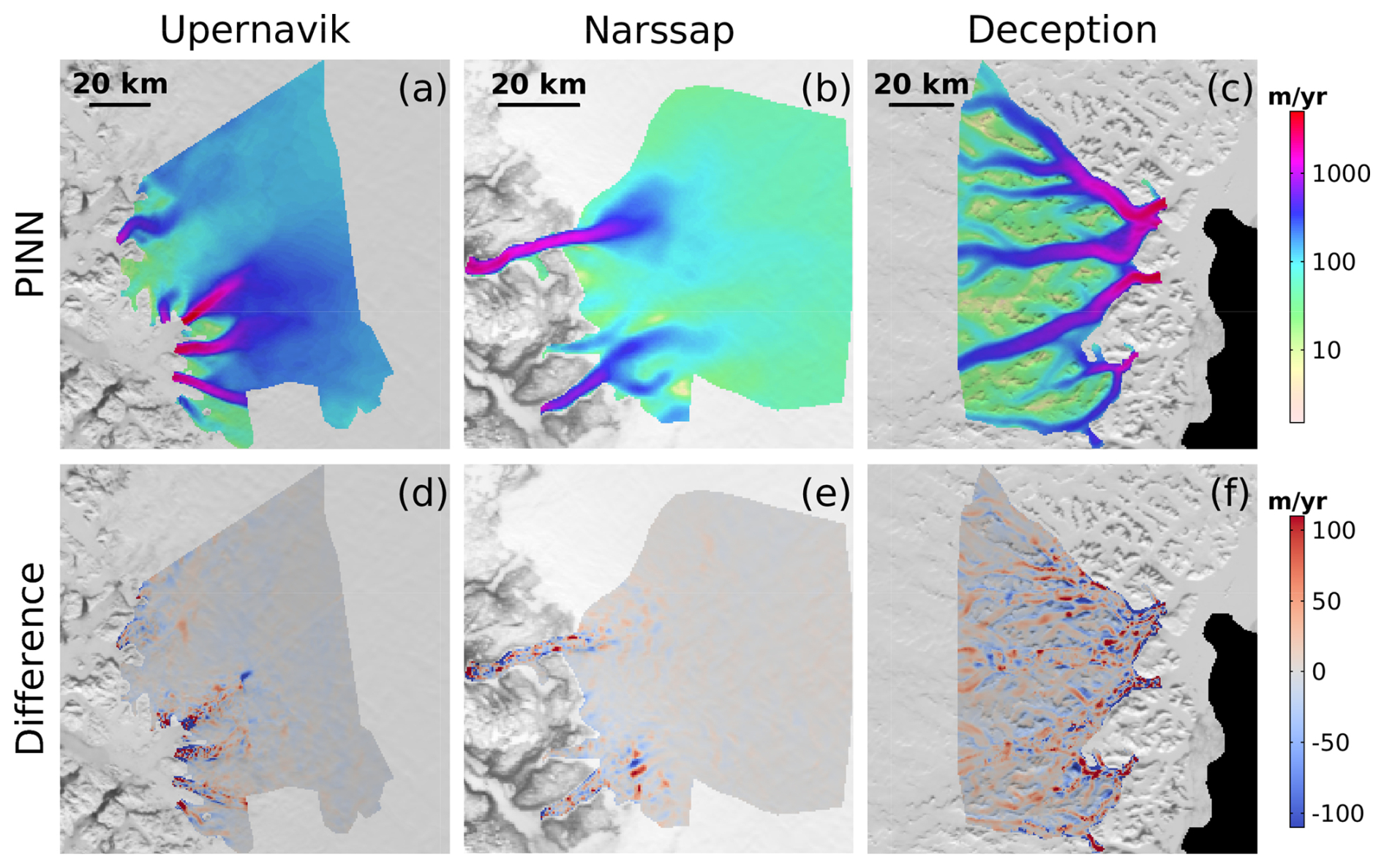
Figure A1 PINN (MB + SB) predicted ice velocity and difference maps for (a, d) Upernavik, (b, e) Narssap, and (c, f) Deception. (a)–(c) depict the PINN (MB + SB) predicted ice velocity maps and (d)–(f) depict the difference between ice velocity from NASA MEaSUREs shown in Fig. 2a, e, i and PINN velocity maps.

PINN (MB + SB) predicts the apparent mass balance, or the linear combination of surface mass balance and ice thinning rates, ($\dot{a}$) for each region as shown in Fig. A2a–c. These predictions are used in the $\dot{a}$ data loss and mass balance physical loss term of the loss function (${\mathcal{L}}_{\dot{a}},{\mathcal{L}}_{{\mathit{\phi }}_{\text{MB}}}$ in Eq. 15). To evaluate how closely the PINN captures $\dot{a}$, we calculate the difference between the training data from RACMO 2.3 (Noël et al., 2016) and ICESat-2 derived ice thinning rates (Smith et al., 2020) and the predicted values; these difference maps are shown in Fig. A2d–f. The difference maps show that the PINN successfully captures $\dot{a}$ (RMSEs and FRMSEs shown in Table 5) within an RMSE of 0.5 m yr⁻¹ and an FRMSE of 10 % for all three regions. Narssap and Deception $\dot{a}$ predictions have lower RMSEs of 0.0209 and 0.0321 m yr⁻¹ respectively, while the Upernavik $\dot{a}$ prediction has an RMSE that is an order of magnitude higher at 0.112 m yr⁻¹.

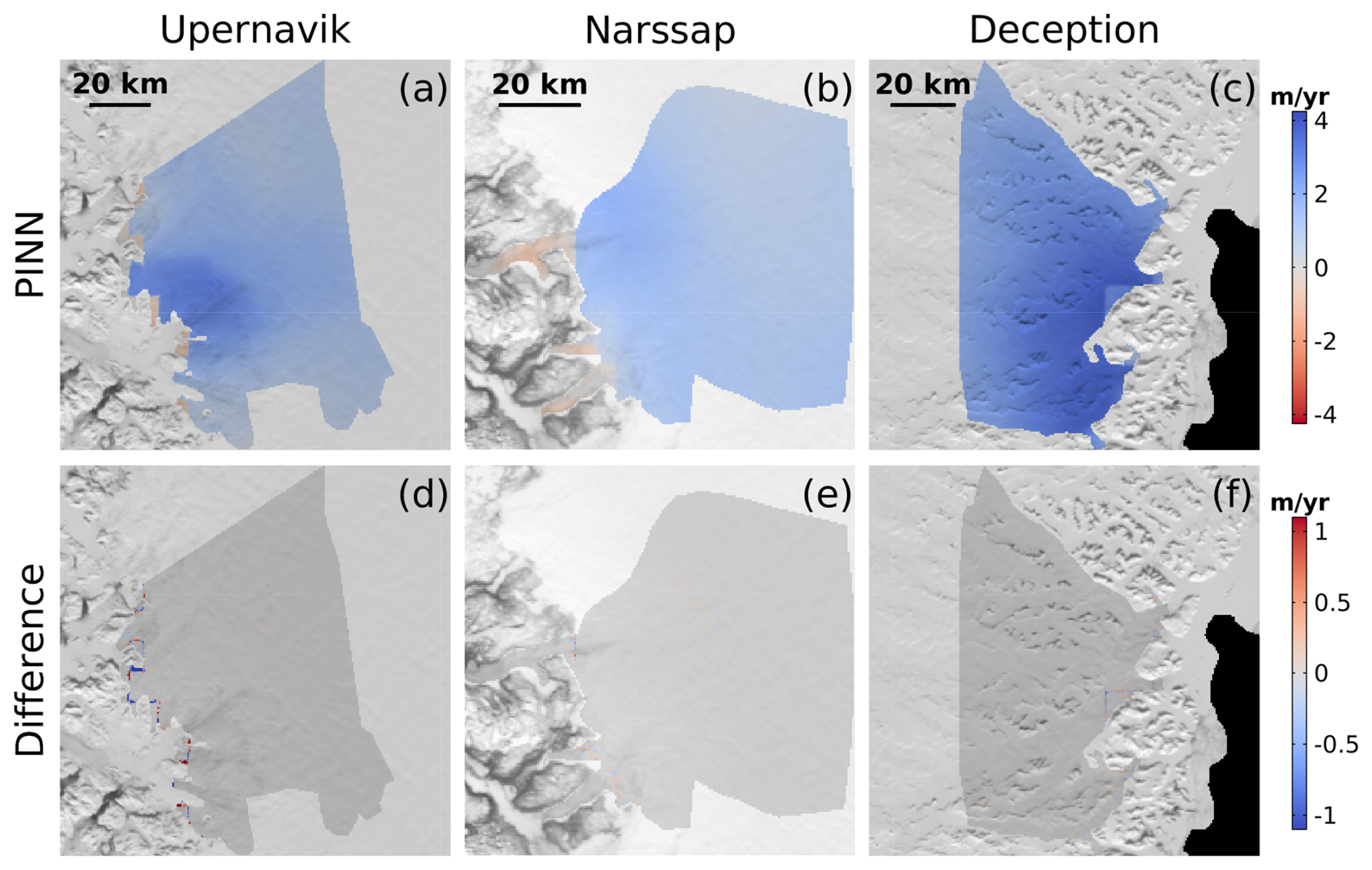
Figure A2 PINN (MB + SB) predicted $\dot{a}$ and difference maps for (a, d) Upernavik, (b, e) Narssap, and (c, f) Deception. (a)–(c) depict the PINN (MB + SB) predicted $\dot{a}$ maps and (d)–(f) depict the difference between $\dot{a}$ derived from RACMO 2.3 and ICESat-2 shown in Fig. 2b, f, j and the PINN $\dot{a}$ maps.

PINN (MB + SB) also predicts the surface elevation for each region, shown in Fig. A3a–c. These predictions are used in the surface elevation data loss and stress balance physical loss term of the loss function (${\mathcal{L}}_s,{\mathcal{L}}_{{\mathit{\phi }}_{\text{SB}}}$ in Eq. 15). To evaluate how well the PINN predicts the surface elevation, we calculate the difference between the surface elevation training data from GIMP (Howat et al., 2014) and the predicted surface elevation, shown in Fig. A3d–f. While the difference maps show that the PINN does generally capture the surface elevation (RMSEs and FRMSEs are shown in Table 5), these maps also suggest that the PINN predictions yield a far smoother surface elevation profile than GIMP. Even so, the FRMSE values for all three regions are within 5 %, suggesting that the PINN is capable of capturing the general, lower frequency approximation of the surface elevation. Upernavik and Narssap surface elevation predictions have lower RMSEs of 20.9 and 12.3 m respectively, while the Deception surface elevation prediction has a higher RMSE of 56.2 m.

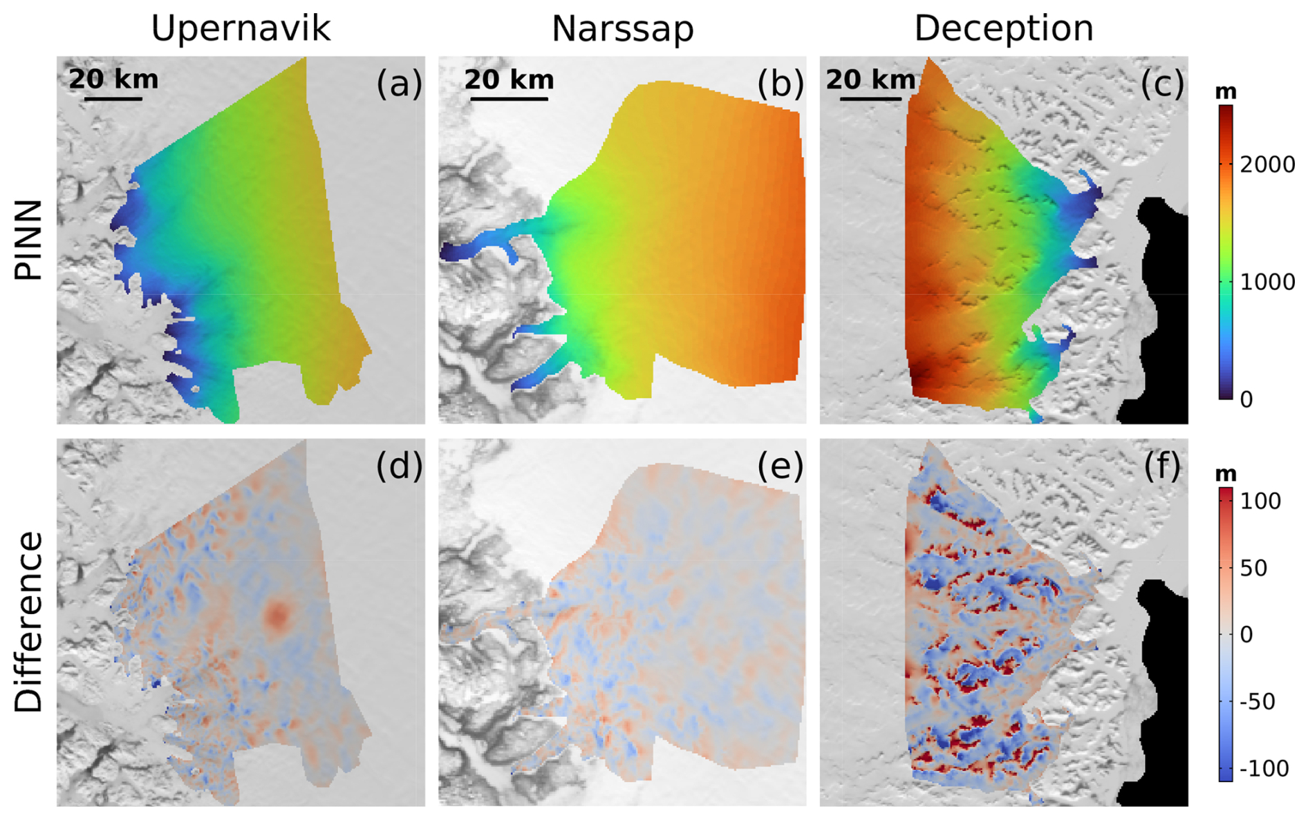
Figure A3 PINN (MB + SB) predicted surface elevation and difference maps for (a, d) Upernavik, (b, e) Narssap, and (c, f) Deception. (a)–(c) depict the PINN (MB + SB) predicted surface elevation maps and (d)–(f) depict the difference between surface elevation from GIMP shown in Fig. 2c, g, k and PINN surface elevation maps.

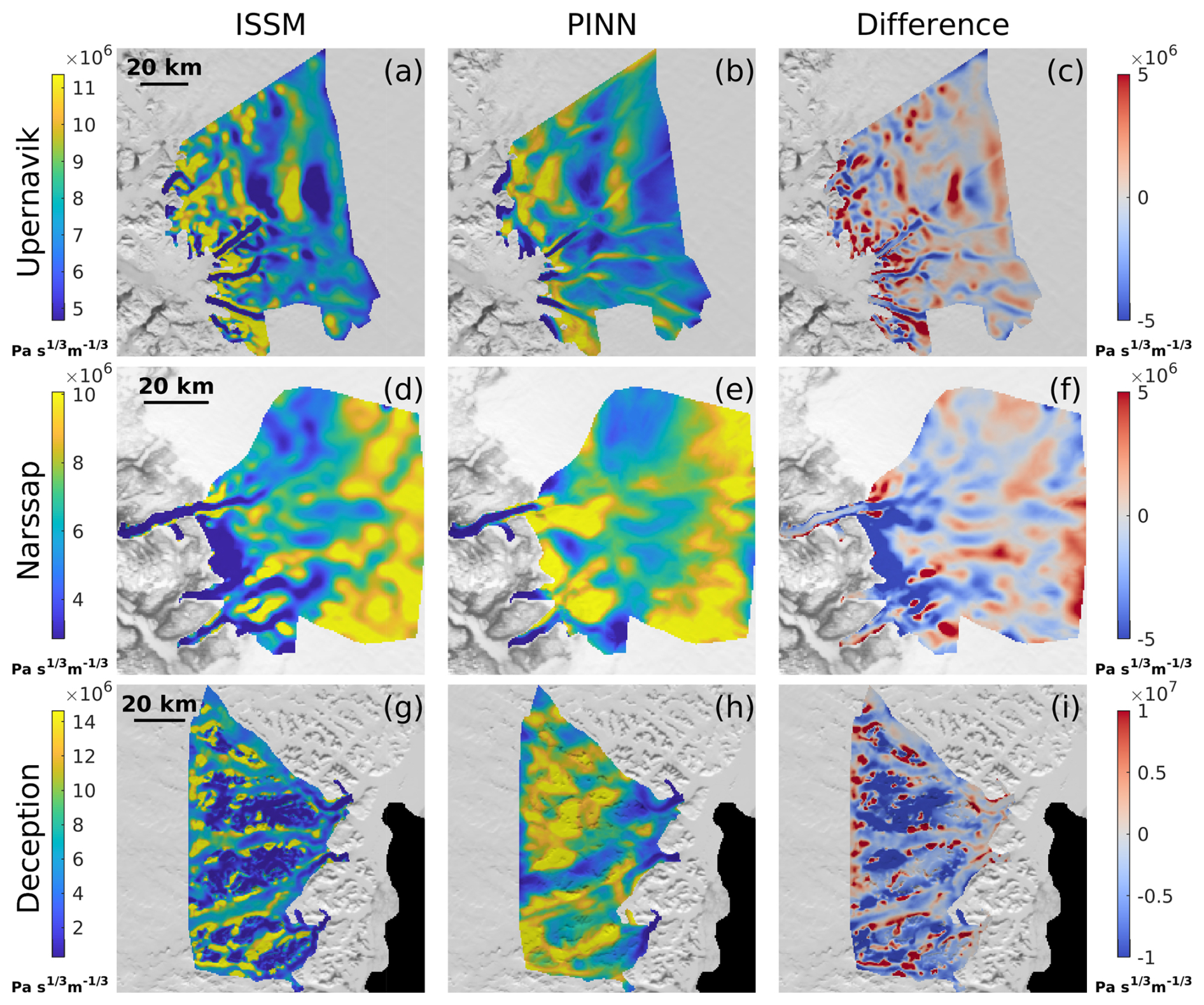
Figure A4 Squared basal friction coefficients and difference maps for (a–c) Upernavik, (d–f) Narssap, and (g–i) Deception. (a), (d), (g) depict the ISSM inverted squared basal friction coefficients, (b), (e), (h) depict the PINN (MB + SB) predicted squared basal friction coefficients, and (c), (f), (i) depict the difference between the inverted and predicted squared basal friction coefficients.

In addition to the aforementioned observable features, PINN (MB + SB) also predicts the basal friction coefficients for each region. These predictions are used only in the stress balance loss terms of the loss function(${\mathcal{L}}_{{\mathit{\phi }}_{\text{SB}}}$ in Eq. (15). Since we do not provide the PINN with any training data for the basal friction coefficients, to assess the quality of PINN predictions we invert for the basal friction coefficients using the Ice-sheet and Sea-level System Model (ISSM, Larour et al., 2012) with the method described in Morlighem et al. (2013). Note that to obtain the inverted basal friction coefficients, we initialize our ISSM models with BedMachine (version 6) ice thickness values. Given the formulation of Weertman's friction law, Eq. (6), we plot maps of the PINN predicted squared basal friction coefficient values (C²) that are used to calculate the basal shear stress (Eq. 6); these are shown in Fig. A4b, e, h. Figure A4a, d, g depict the squared basal friction coefficient values ($C_{\text{ISSM}}^{\mathrm{2}}$) obtained through an inversion using ISSM. The differences between these two squared basal friction coefficient maps are shown in Fig. A4c, f, i.

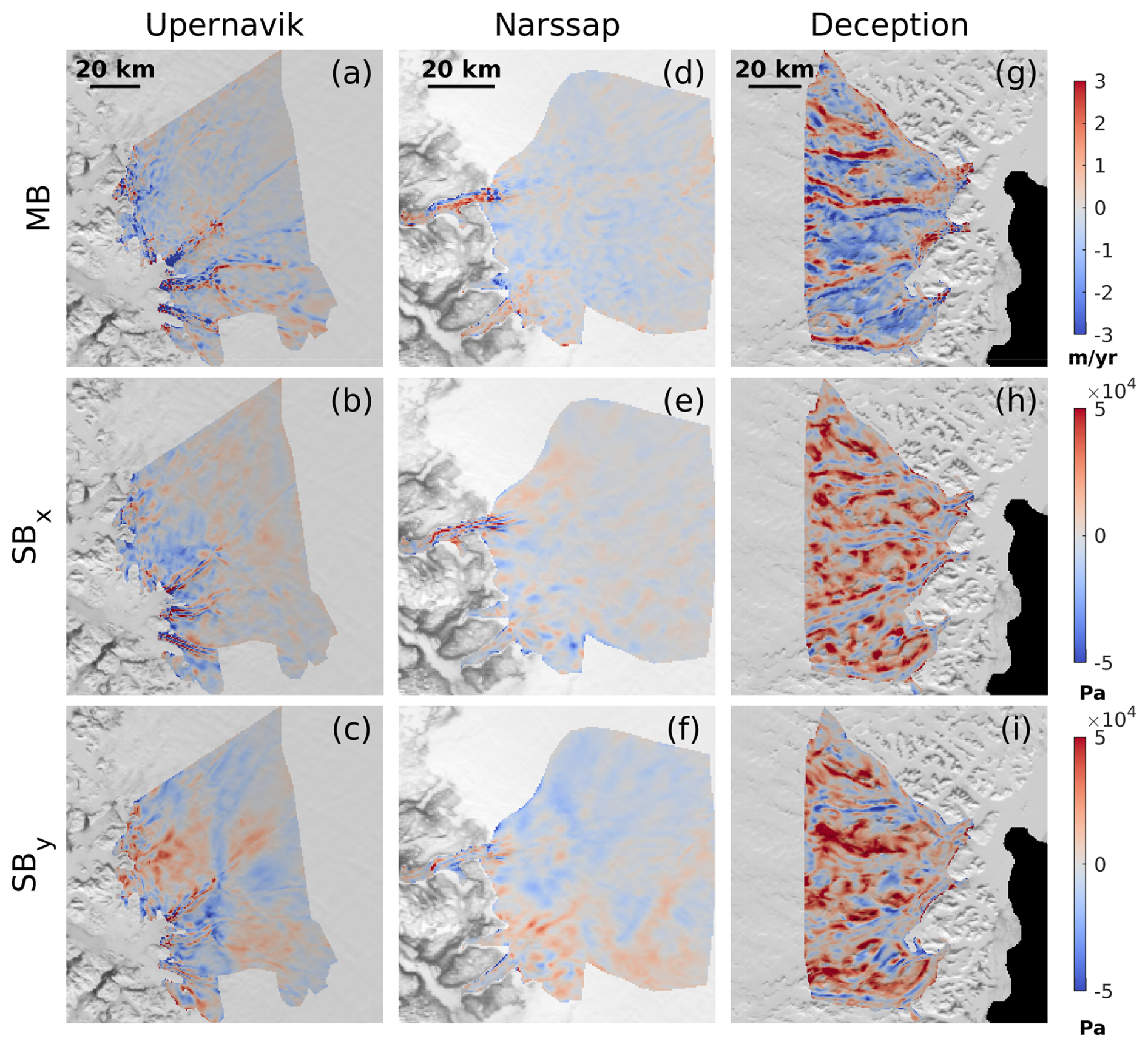
Figure A5 Predicted variables from PINN (MB + SB) substituted into the PDE residuals for (a, b, c) Upernavik, (d, e, f) Narssap, and (g, h, i) Deception. We compute the (a, d, g) mass balance residuals (Eq. 3) as well as the (b, e, h) stress balance residuals in x and the (c, f, i) stress balance residuals in y (Eq. 4) for each region of interest.

We observe that the inverted and predicted squared basal friction coefficients for Upernavik and Narssap share some similarities, with lower coefficients in regions of fast-flowing ice and higher coefficients in regions where the ice is slower-moving. However, we also observe these maps have notable differences of $\sim \mathrm{5}\times {\mathrm{10}}^{\mathrm{6}}$ Pa s${}^{\mathrm{1}/\mathrm{3}}$ m${}^{-\mathrm{1}/\mathrm{3}}$ located in the areas of fast-flowing ice. For Deception, we observe that the squared basal friction coefficient maps are significantly different, especially in the region where the PINN predicts an intricate network of troughs, outside the MC domain, where the PINN bed topography is over 600 m deeper than that of BedMachine.

Lastly, we substitute these values back into the PDE residual terms of our loss function, ${\mathcal{L}}_{{\mathit{\phi }}_{\text{MB}}},{\mathcal{L}}_{{\mathit{\phi }}_{\text{SB}}}$ to assess how well the PINN (MB + SB) predictions are satisfying the physical laws. Figure A5a, d, g depict the mass balance residuals for each region, which are generally the same order of magnitude as the mass balance typical value, ∼ 1 m yr⁻¹ (see Table 1). Figure A5b, e, h depicts the stress balance residual in x while Fig. A5c, f, i depicts the stress balance residuals in y for all three regions. These values are generally an order of magnitude smaller than the typical values for stress balance, ∼10⁵ Pa (see Table 1). These residual maps suggest that the PINN (MB + SB) is indeed minimizing the PDE residuals and constraining predictions of the state variables such that the PDEs are satisfied, especially in slow-moving regions. We find that the PDE residuals tend to be greater near the fast-flowing regions (which is especially evident for Upernavik, Fig. A5a, b, c), which likely arises since the PINN struggles to capture sharp transitions in the ice velocity.

A2 Extended Discussion

While the focus of this paper is on PINN predictions of the ice thickness, and subsequently the bed topography, we briefly discuss PINN (MB + SB) predictions of our second unknown: the basal friction coefficient. From Fig. A4, we observe that though the inverted and predicted basal friction coefficients share some similarities, there are significant differences that likely occur for a few reasons. First, since the PINN has no training data with which to constrain its predictions for the basal friction coefficient, it must rely solely on the PDE constraints. Yet, as established earlier, there are often uncertainties associated with the PINN predictions of observable ice sheet features that are substituted into the PDE residuals, especially along fast-flowing ice streams, as shown in Fig. A5. Second, we expect that some of the difference in the basal friction coefficients can be explained by the PINN model resolution. Since the PINN is relying solely on the PDE constraints to infer the basal friction coefficients, it will only compute these for the randomly selected collocation points within a region of interest. Therefore, we expect that increasing the number of collocation points (i.e., increasing the PINN model resolution) could improve PINN predictions of the basal friction coefficients. Lastly, minor differences could be explained by the differences in model geometries as the inverted basal friction coefficients rely on BedMachine ice thickness while the PINN basal friction coefficients use the PINN predicted ice thickness. Indeed, we observe that there is a significant difference in bed topography of over ∼600 m in the northwest sector of the Deception region, where we also observe that the difference in basal friction coefficients is more pronounced (see Figs. 5f and A4).

Appendix B: Validation

B1 Effect of Ice-Penetrating Radar Track Spacing

We assess the accuracy of our PINN (MB + SB) framework by training a PINN (coupling mass balance and stress balance) for the Upernavik region shown in Figs. 2a–d and 3a. We find this region to be appropriate for a validation study as the bed topography is well constrained with dense ice thickness measurements as shown in Fig. 2d. We create three distinct validation experiments, each of which involves training a PINN using randomly selected data points from a subset of the available ice thickness measurements along ice-penetrating radar flight tracks with different spacing and keep the rest of the ice thickness measurements “hidden”. The “hidden” measurements will be used later for testing the accuracy of PINN predictions within the region of interest.

B2 Experiment 1 (∼15 km)

We keep a subset of ice-penetrating radar flight tracks for training (i.e., the black flight tracks in Fig. B1d that are ∼15 km apart) and keep the rest “hidden” (i.e., the yellow flight tracks in Fig. B1d). Most notably, we hide majority of the ice thickness measurements along Upernavik Isstrøm North to ascertain whether the PINN can infer the trough beneath from sparse ice thickness observations. Henceforth we refer to the PINN trained for this experiment as “PINN (V1)” (or the validation PINN 1).

B3 Experiment 2 (∼30 km)

We assess how well the PINN performs with sparse ice thickness data, we reduce our training data set to three flight tracks (that are oriented across the flow direction) ∼30 km apart within in the Upernavik region, as shown by the black flight tracks in Fig. B1e. We keep all other flight tracks “hidden” for testing the PINN predictions. Henceforth we refer to the PINN trained for this experiment as “PINN (V2)” (or the validation PINN 2).

B4 Experiment 3 (∼60 km)

We expose the PINN to a single flight track close to the inflow boundary within the Upernavik region, ∼60 km from the outflow boundary, indicated by the black flight track in Fig. B1f. We keep all other flight tracks “hidden” for testing the PINN predictions. Henceforth we refer to the PINN trained for this experiment as “PINN (V3)” (or the validation PINN 3).

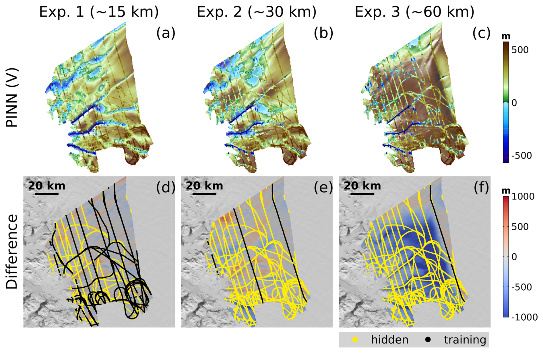
Figure B1 Results of the PINN validation experiments for the Upernavik region. (a), (b), (c) show the PINN predicted bed topography maps for each validation experiment, which we overlay with ground-truth bed topography data calculated along ice-penetrating radar flight tracks. (d), (e), (f) show the difference between BedMachine and PINN bed topography maps, b_BedMachine−b (m). We also plot the subset of flight tracks from which we select data points for training the validation PINNs (i.e., PINN (V)) as black lines and the subset of flight tracks that are hidden for validation as yellow lines on the difference maps. (a, d) Experiment 1, the PINN is trained using only a subset of the ice thickness measurements, most of the data is hidden along Upernavik Isstrøm North. (b, e) Experiment 2, the PINN is trained using only three flight tracks, while the rest are hidden. (c, f) Experiment 3, the PINN is trained using ice thickness data along a single flight track, close to the inflow boundary of the Upernavik region.

Table B1 RMSEs for the each of the distinct experiments in the validation study along “training” and “hidden” ice-penetrating radar flight tracks for the Upernavik region.

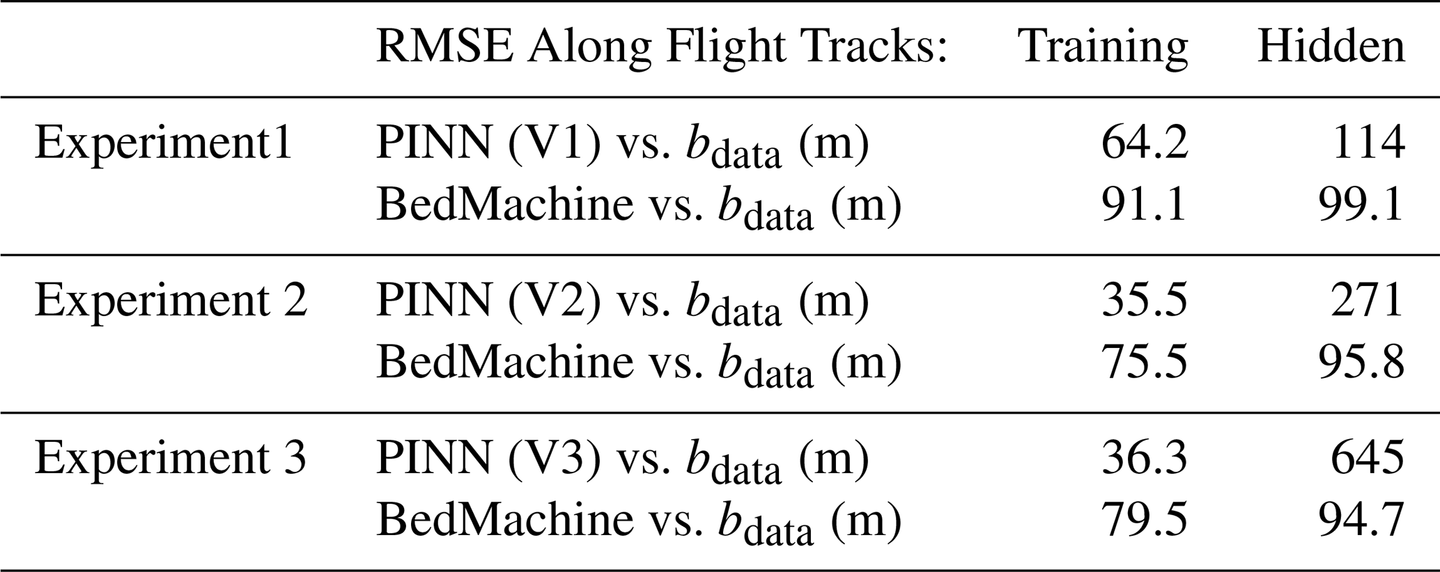
We compare the PINN (V1), PINN (V2), and PINN (V3) predictions to ground-truth bed topography data ${\widehat{\mathit{b}}}_{\text{data}}$, calculated along ice-penetrating radar flight tracks. Table B1 shows the RMSEs between ground-truth and predicted bed topography values along the training and hidden ice-penetrating radar flight tracks. For comparison, we also include the RMSEs between ground-truth and BedMachine bed topography values in Table B1.

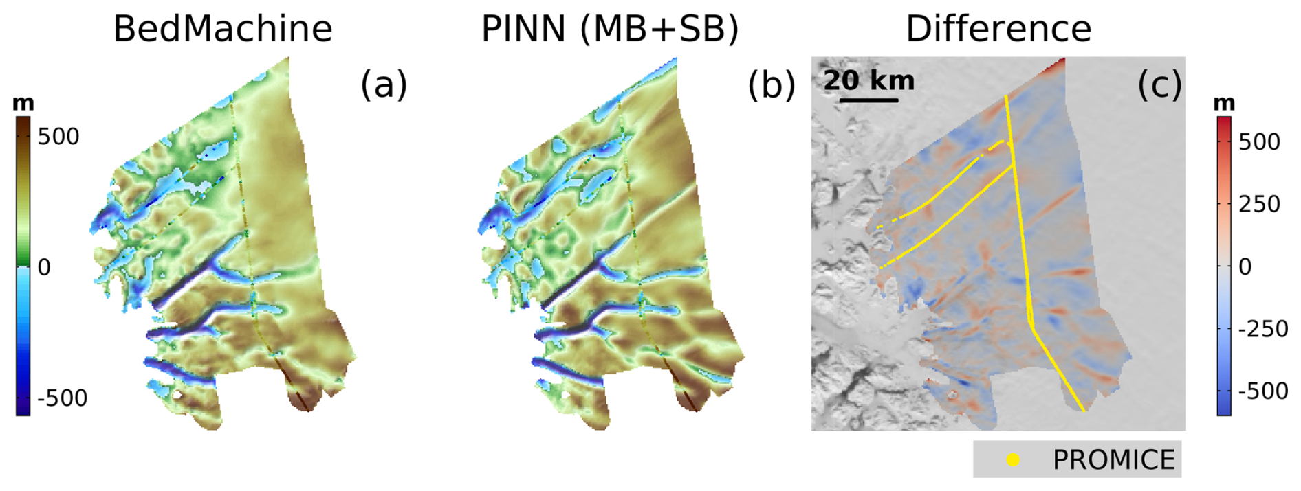
Figure B2 Comparison of PINN (MB + SB) predictions with independent ice thickness data set. we show the bed topography maps of (a) BedMachine (version 6) and (b) PINN (MB + SB) (i.e., our main results from Fig. 5a), which we overlay with PROMICE ice thickness data. (c) shows the difference between BedMachine and the PINN bed topography maps, b_BedMachine−b (m). We also plot the PROMICE flight track, where we have ice thickness data, on the difference map (i.e., the yellow lines).

PINN (V1) predicts a bed topography map, shown in Fig. B1a, that is similar to that of BedMachine, with differences less than ∼ 250 m. Despite being exposed to randomly sampled ice thickness measurements from the training subset (black lines only) of flight tracks in Fig. B1d situation ∼15 km apart, we find that PINN (V1) is able to recover a trough along Upernavik Isstrøm North. Along the training flight tracks for Experiment 1, the PINN (V1) RMSE of 64.2 m is lower than the BedMachine RMSE of 91.1 m, implying that PINN (V1) is satisfying the ground-truth observations better than BedMachine. However, along the hidden flight tracks (for the same experiment), we observe that the PINN (V1) RMSE of 114 m is slightly higher than the BedMachine RMSE of 99.1 m. This is likely because Bedmachine has been exposed to all the ice thickness measurements along the hidden flight tracks, whereas PINN (V1) has been exposed to none of these measurements. Given that BedMachine has been exposed to all the hidden flight tracks and the PINN (V1) has been exposed to none of them, we find it highly promising that these RMSEs are similar. The results of this experiment reveal that by coupling mass balance with stress balance in our PINN framework, we are indeed able to predict a realistic bed topography using observable ice sheet features and sparse ice thickness measurements.

Even though PINN (V2) is only exposed to three flight tracks that are situated ∼ 30 km apart during the training process (Fig. B1e), we find that PINN (V2) predicts a bed topography map with differences of less than ∼ 400 m compared to BedMachine (Fig. B1b). Most importantly, PINN (V2) successfully recovers troughs beneath Upernavik Isstrøm North, Upernavik Isstrøm Central, and Upernavik Isstrøm South. PINN (V2) does predict a disjointed trough beneath Nunatakassaap Sermia, but this is to be expected since it is not exposed to much ice thickness data along flow. Along the training flight tracks for Experiment 2, the PINN (V2) RMSE of 35.5 m is significantly lower than the BedMachine RMSE of 75.5 m. Similar to the trend we observed in Experiment 1, along the hidden flight tracks for Experiment 2, the PINN (V2) RMSE of 271 m is greater than the BedMachine RMSE of 95.8 m. This could be explained in part by the fact that BedMachine has been exposed to all the ice thickness measurements along the hidden flight tracks and PINN (V2) has been exposed to none of these. Another reason for the high PINN (V2) RMSE (along hidden flight tracks) could be that the PINN is exposed to limited data along flow, meaning that its predictions are not as well constrained. Still, we find it promising that even with as few as three flight tracks of training data, PINN (V2) has successfully recovered the general bed characteristics of the Upernavik region.

For Experiment 3, PINN (V3) is exposed to data only along one flight track near the inflow boundary of the Upernavik region and predicts an unrealistic bed topography with much thinner ice, as shown in Fig. B1c, f. We find that PINN (V3) does not recover the troughs beneath Upernavik Isstrøm North, Upernavik Isstrøm Central, and Upernavik Isstrøm South, as well as the trough beneath Nunatakassaap Sermia. While PINN (V3) predictions along the training flight tracks are fairly well constrained (as indicated by the low RMSE of 36.3 m in Table B1), the predictions along the hidden flight tracks are not close to the measured bed topography values (as shown by the high RMSE of 645 m). We expect that this is because PINN (V3) does not have enough data along flow to constrain its predictions, implying that the PINN (MB + SB) architecture needs ice thickness measurements from at least one more flight track within the region of interest.

B5 Validation using Independent Data: PROMICE

We further validate our PINN (MB + SB) framework by comparing our main result (Fig. 5a) to ground-truth bed topography derived using ice thickness measurements from the PROMICE airborne surveys (Sandberg Sørensen et al., 2018). Since the PINN (MB + SB) is trained only using ice thickness data from CReSIS radar depth sounder data (CReSIS, 2016), the ice thickness measurements from the PROMICE airborne surveys provides an independent data set for validation. Figure B2a, b depict the bed topography maps from BedMachine Greenland (version 6) and PINN (MB + SB) respectively, which we overlay with ground-truth bed topography data calculated using ice thickness measurements along the PROMICE flight track. Figure B2c depicts the difference between BedMachine and PINN (MB + SB), with the PROMICE flight track plotted in yellow.

Table B2 RMSEs for the validation study on Upernavik using an independent ice thickness data set from PROMICE airborne surveys.

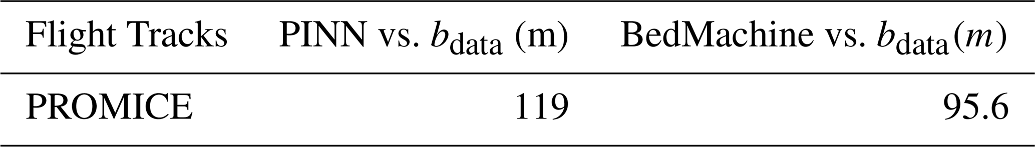
As indicated in Table B2, the RMSE in PINN (MB + SB) predictions compared to ground-truth PROMICE data is 119 m, which is slightly higher than the RMSE of 95.6 m between BedMachine and PROMICE data. We note that the BedMachine RMSE is likely lower since it has been exposed to all of the PROMICE ice thickness data whereas the PINN has been exposed to none of these. Even so, we find that the similar RMSEs suggest that the PINN (MB + SB) framework successfully resolves the bed topography along the PROMICE flight track, despite not being exposed to the ice thickness data.

Appendix C: Resampling of Collocation Points

Resampling the collocation points (on which the PDE residuals are evaluated) during the training process is possible in the PINNICLE package (Cheng et al., 2025b). However, using this resampling technique can add to the computational cost because resampling the collocation points often leads to slower convergence. In our experiments, we have instead opted to use a high number of collocation points (N_φ=9000), to ensure good coverage and ensure that the physical laws are generally conserved throughout the region. Since we train an ensemble of five PINNs (each initialized with different random seeds, resulting in different collocation points chosen for each) and retrieve the median prediction, we expect this final result to be similar to the result of a PINN trained with resampling of collocation points.

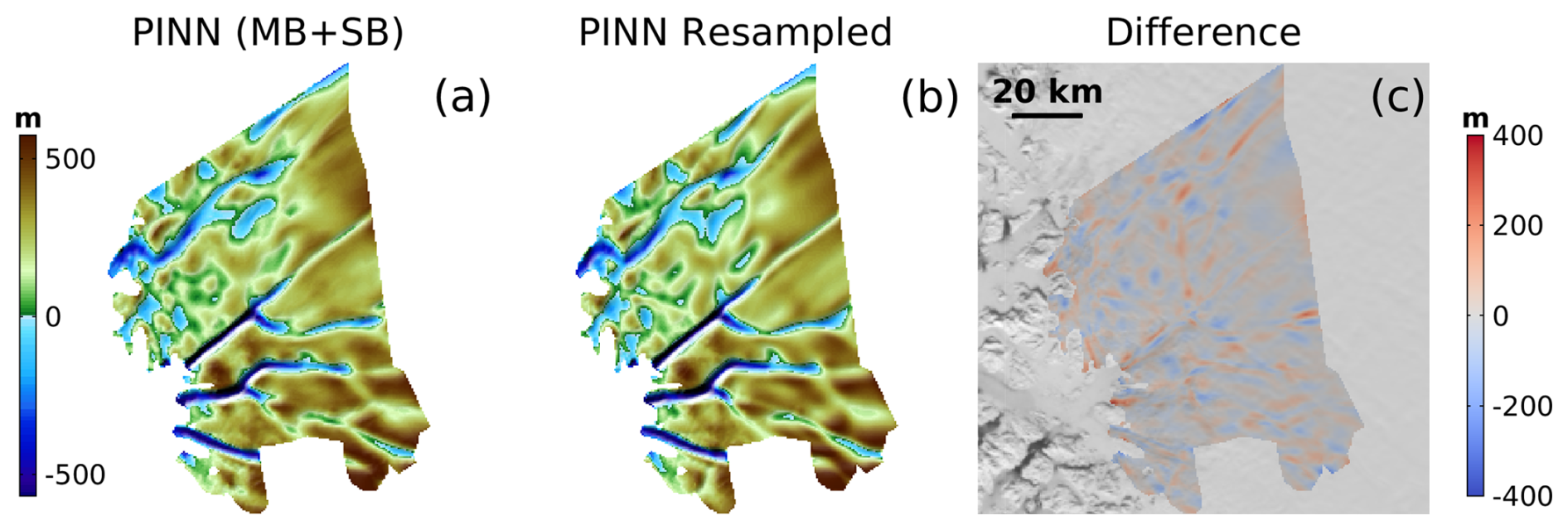
Figure C1 Bed topography for the Upernavik region from (a) ensemble PINN (MB + SB) predictions and (b) PINN (coupling mass balance and stress balance) with re-sampling every 100 iterations. (c) shows the difference between these two maps, $b_{\text{PINN }(\mathrm{MB}+\mathrm{SB})}-b_{\text{PINN Resampled}}$.

To that end, we train a single PINN (with coupled mass balance and stress balance) for the Upernavik region, using 4000 collocation points that are resampled every 100 iterations. All other model parameter choices, including number of data points, total number of iterations, and loss function weights, are retained from the PINN (MB + SB) experiment. The result of this resampling experiment is shown in Fig. C1b. Comparing this with our ensemble PINN (MB + SB) bed topography prediction for Upernavik, Fig. C1a, we note that differences between these two bed topography maps are ∼200 m, as shown in Fig. C1c.

The highly similar bed topography maps in Fig. C1a, b suggest that the ensemble PINN (MB + SB) and the PINN trained with resampling of collocation points yield similar results. We note that resampling is indeed a powerful implementation as the result of a single PINN is highly similar to our ensemble prediction using five PINNs. This is to be expected since collocation points are resampled every 100 iterations (out of a total of 700 000 iterations), leading to a better coverage for the entire region of interest. Interestingly, with the resampling, though the PINN prediction is “smoother” (not capturing much realistic bed roughness), we see that it is closer than the ensemble PINN (MB + SB) in recovering the trough beneath the Southern Fork of Upernavik Isstrøm North. Therefore, an ensemble PINN prediction may still be necessary to resolve finer-scale bed roughness details.

Appendix D: Comparison to an Independent Bed Topography Product

We compare the PINN (MB + SB) predicted bed topography to an independent bed topography product generated using another machine learning, quantile regression forest (QRF) approach (Palmer et al., 2025). For the Deception region, the QRF bed topography is highly similar to that of the PINN predicted bed topography. Both maps show an intricate network of troughs that coincide with the fast-flowing ice streams in the region (as shown in Fig. D1). We also find that the QRF approach better captures the depth of the troughs beneath Deception Ø Central North, Deception Ø Central South, and Uunartit Islands, similar to BedMachine. The QRF map for the Upernavik region is fairly similar to that produced by PINN approach (as shown in Fig. D1). Similar to the PINN, the QRF approach predicts a discontinuous trough beneath the southern fork of Upernavik Isstrøm North, perhaps implying the need for more data in this region to better constrain the bed topography. However, unlike the PINN approach, the QRF approach predicts a discontinuous trough beneath Nunatakassaap Sermia. For the Narssap region, we find that the QRF approach and the PINN approach yield completely different bed topography maps, as the QRF approach does not seem to detect the presence of a trough beneath Narssap Sermia, which is present in both BedMachine and the PINN predicted bed topography.

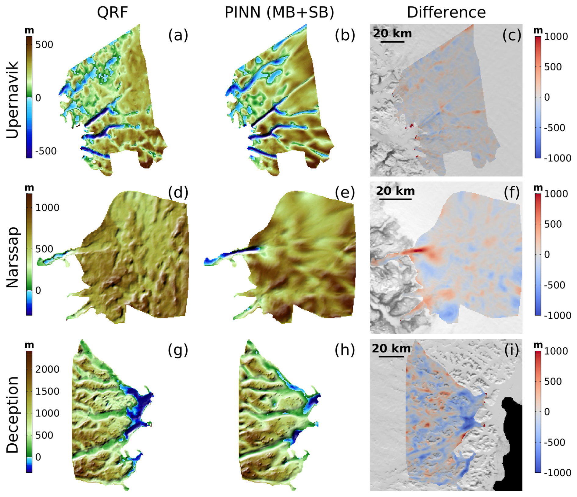
Figure D1 Comparison of PINN (MB + SB) predictions with the Quantile Regression Forest (QRF) approach to estimating the bed topography (Palmer et al., 2025) for the (a, b, c) Upernavik, (d, e, f) Narssap, and (g, h, i) Deception regions. (a), (d), (g) depicts the QRF bed topography maps, (b), (e), (h) depicts the PINN (MB + SB) bed topography predictions, and (c), (f), (i) depict the differences between the QRF and the PINN (MB + SB) bed predictions, ${\widehat{\mathit{b}}}_{\text{QRF}}-\widehat{\mathit{b}}$ (m).