Detection and attribution of the role of anthropogenic climate change in industrial-era retreat of Pine Island Glacier

The West Antarctic Ice Sheet (WAIS) has undergone rapid change over the satellite era, characterized by significant thinning, grounding-line retreat, and mass loss. More than a third of the ice loss from this region is from Pine Island Glacier (PIG). However, robust causal links between anthropogenic climate change and PIG ice loss have yet to be established. Here we attempt to quantify the role of anthropogenic climate change in observed retreat of PIG over the 20th century and how this may evolve up to 2200. To do so, we use an ensemble Kalman inversion data assimilation method embedded into an uncertainty quantification framework, called calibrate-emulate-sample (CES). This procedure, which assimilates observations of grounding-line retreat and ice volume, yields observationally constrained probability distributions of both model and climate forcing parameters. Our analysis suggests that it is unlikely that the extent of 20th century PIG retreat would have taken place without anthropogenically driven trends in ice-sheet forcing and that anthropogenic forcing exacerbated the extent of PIG retreat over the 20th century, by approximately 18 %. These results are, importantly, conditional on our choice of initial state. For our chosen initial state, we find that the parameter combinations compatible with these observational constraints require PIG to lose mass (but not experience grounding-line retreat) over the entire simulated period since 1750, not just after the 1940s when grounding-line retreat was initiated. This preconditioned ice mass loss introduces significant uncertainty into our quantification of 20th century forcing contributions. In simulations with no anthropogenic trend in forcing, we still observe significant retreat; this may result either from a larger-than-actual initial state, or may suggest that the earlier ice state preconditioned the industrial era retreat, possibly implicating longer term changes to WAIS in the present retreat.

1 Introduction

The West Antarctic Ice Sheet (WAIS) has undergone rapid change over the satellite era, characterized by significant ice acceleration (Mouginot et al., 2014), thinning (Smith et al., 2020), grounding-line retreat (Rignot et al., 2014), and mass loss (Rignot et al., 2019). Almost all of the ice loss from the Antarctic Ice Sheet over the satellite era has come from the WAIS (Otosaka et al., 2023). Of this, a majority comes from two major outlet glaciers: the Pine Island and Thwaites Glaciers (Morlighem et al., 2020).

Despite these changes occuring at the same time as anthropogenic climate change, robust causal links between climate change and West Antarctic Ice Sheet loss have yet to be established (Meredith et al., 2019; Fox-Kemper et al., 2021). Several lines of evidence point to contributions to retreat from different sources; these include long, slow retreat since the Last Glacial Maximum, a period of anomolously high forcing in the 1940s which triggered rapid ice loss over the 20th century, internal ice and ocean feedbacks, and anthropogenically driven changes in climatic forcing. We first briefly document this evidence.

1.1 Evidence linking WAIS retreat to anthopogenic forcing

Geological and geophysical evidence implies that at the Last Glacial Maximum (around 25 000 years ago), the West Antarctic Ice Sheet extended close to the continental shelf edge along the Amundsen Sea and Bellingshausen Sea margins (Larter et al., 2014). By around 10 000 years ago, grounding lines in the region had retreated significantly, approaching locations close to the present day (Larter et al., 2014). This retreat, on the order of 500 km over 15 000 years (i.e. approx 33 m per year on average), is much slower than present day retreat rates, which are on the order of several hundred metres per year (Chartrand et al., 2024). Since then, the ice-sheet geometry has remained broadly similar, albeit with localised retreat (Larter et al., 2014), which has accelerated in recent decades. Owing to their large size and high viscosity, ice-sheet response timescales (the timescale on which an ice-sheet responds to changes in climate forcing), are very long, potentially on the order of tens of thousands of years. Therefore, memory of the slow retreat of WAIS since the last glacial maximum may plausibly still be playing a role in its evolution today.

Analysis of sediment cores taken beneath the Pine Island (Smith et al., 2017) and Thwaites (Clark et al., 2024) Glaciers indicates that the present phase of rapid retreat was initiated in the 1940s. They also indicate that Pine Island Glacier was stably grounded on a prominent seabed ridge prior to the 1940s, with the ice shelf finally detaching from the ridge in the 1970s (Jenkins et al., 2010; Smith et al., 2017). Once initiated, a range of ice and ocean feedbacks would have helped to sustain its retreat; these include: grounding-line retreat towards a deeper bed (Favier et al., 2014), increasing ice damage (Lhermitte et al., 2020), increased access of warm water into sub-ice-shelf cavities (De Rydt et al., 2014), retreat of the ice front (Bradley et al., 2022), increased ice base area exposed to warm ocean water (Holland et al., 2023), and spinup of circulation inshore of the ridge (De Rydt and Naughten, 2024). There is evidence that, following its complete unpinning, Pine Island underwent a period of irreversible retreat until the 1990s (Reed et al., 2024a, b). However, the present phase of retreat cannot be purely self-sustaining because ice discharge remains responsive to ocean forcing (Christianson et al., 2016; Jenkins et al., 2018).

During the initial retreat in the 1940s, high pressure and wind over the Amundsen Sea Embayment (Schneider and Steig, 2008) are thought to have driven increased warm Circumpolar Deep Water (CDW) access to ice shelf cavities and therefore increased ice shelf basal melting (Steig et al., 2012). Increases in basal melting reduce the restraining back-pressure (“buttressing”) that ice shelves apply to the adjacent ice-sheet (Shepherd et al., 2004; Pritchard et al., 2012). O'Connor et al. (2023) demonstrated that, although the pressure and wind anomalies in the 1940s are exceptional in the context of the past century, they are not exceptional in the context of the last 10 000 years: an event of this magnitude would have occurred tens to hundreds of times over the last 10 000 years. Thus, the 1940s event is unlikely to be solely responsible for the current phase of retreat: events of this magnitude have taken place many times before, but have not initiated ongoing rapid centennial scale retreat.

This raises the question: why did the increase in CDW in the 1940 event initiate retreat? And, to what extent were anthropogenic trends in forcing responsible? Proxy-constrained climate simulations suggest that westerly winds at the Amundsen Shelf break were changing over the 20th century (Holland et al., 2019), but the anthropogenic (rather than internal) component of this trend only emerged in the 1960s (Holland et al., 2022). Trends in westerly winds over the Amundsen Sea are a well established response of the Southern Hemisphere climate to anthropogenic emissions (e.g. Arblaster and Meehl, 2006). In ocean simulations, these wind changes drive CDW under the ice shelf cavities more frequently on decadal timescales, increasing ice shelf melting (Naughten et al., 2022). One plausible narrative is that WAIS retreat may have been triggered in the 1940s by naturally occuring climate change, but was then sustained by anthropogenic climate forcing since the 1960s. Without this change, WAIS might have recovered, as it appears to have done many times before in the past (Holland et al., 2022; O'Connor et al., 2023).

1.2 Challenges in attributing West Antarctic Ice Sheet retreat

In this study, we aim to quantify the role of anthropogenic trends in forcing on retreat of the Pine Island Glacier (PIG). We focus on PIG specifically (rather than the whole of the WAIS) because of the availability of grounding-line constraints prior to the satellite era (Smith et al., 2017) and because using a smaller domain reduces computational expense in the large ensemble of model simulations required. As in other attribution studies (e.g. Otto, 2017), we compare simulations of PIG response under all climate forcings with simulations under only natural forcings, aiming to reproduce the behaviour of the glacier since 1750. We take a probabilistic approach, as in other studies, to account for uncertainties in climatic forcing, model parameters, and future forcing scenarios (Bradley et al., 2024b).

There are three key challenges to address. First, simulations of ice sheet change are sensitive to choices of model parameters, some of which are very poorly-constrained. This makes reconstructing the magnitude and timing of PIG retreat challenging because only a small subspace of model parameter values are compatible with the observed retreat (discussed further in “Methods”). Simulations in idealized geometries indicate that ice sheet retreat attribution assessments are highly sensitive to the choice of fixed model parameters (Christian et al., 2022). Therefore, parametric uncertainty (that arising from poorly constrained model parameters) must be explicitly included in attribution assessments (Bradley et al., 2024b).

Second, evaluation of past ice sheet simulations is usually limited by a lack of data before the satellite era (i.e. around 1979). Here, our focus on PIG allows us to use the sediment-based records of grounding-line location change from the 1940s to 2010 (Smith et al., 2017) to constrain the ice-sheet model parameter distributions.

Finally, changes in Southern Ocean since 1750 are very poorly-known. We therefore use an ensemble of ocean forcing realisations, as in previous studies (Naughten et al., 2022, 2023), to include this aleatoric uncertainty (Robel et al., 2019; Aschwanden et al., 2021). The anthropogenic trend in ocean forcing is treated as an unknown parameter to be inferred in the attribution study: in this way, we learn what the anthropogenic forcing must have been in order to reproduce the past.

The issue of sensitivity of ice sheet model behaviour to poorly constrained model parameters has led to the use of observations of past ice sheet change to constrain model parameters, typically using Bayesian weighting (e.g. Ritz et al., 2015; Nias et al., 2019, 2023; Bevan et al., 2023; Wernecke et al., 2020; Coulon et al., 2024) or history matching (McNeall et al., 2013; DeConto and Pollard, 2016; Edwards et al., 2019). Essentially, the idea is to sample model parameters and then simulate ice sheet behaviour over the historical period using each of these. The parameter sets are then calibrated, either by weighting them (in the case of Bayesian weighting) or by ruling out certain combinations (history matching) based on their agreement with observations over the historical period. When combined with model-emulation (constructing a computationally cheap surrogate emulator of the expensive simulator), observationally-constrained distributions of model parameters can be obtained (e.g. Aschwanden and Brinkerhoff, 2022; Rosier et al., 2024; Jantre et al., 2024; Berdahl et al., 2020). One issue with such parameter sampling is that when the likely parameter space (the region of parameter space where model output agrees with observations) is small, it may be only sampled with a small number of simulations, or not at all. This is particularly pertinent when large numbers of model parameters are involved or systems are non-linear (ice-sheet models have both of these features).

In this paper, we overcome this sampling challenge by using an ensemble Kalman Inversion (EKI) sampling strategy, within an uncertainty quantification framework – “calibrate-emulate-sample” (outlined in “Methods”). Rather than selecting all parameter samples at the outset (i.e. before any simulations are performed, as is typical in ice-sheet modelling), the EKI is an iterative method: the model parameters sampled are updated iteratively based on agreement between previous model simulations and observations. The EKI also benefits from being a gradient-free optimization method: it is not necessary to compute the gradient of the model–observable error with respect to model parameters (Garbuno-Inigo et al., 2020; Kovachki and Stuart, 2019) in order to perform the update. The EKI has been successfully applied to calibrate model parameters in climate models (e.g. Dunbar et al., 2021; Mansfield and Sheshadri, 2022; King et al., 2024), but we believe this is its first application in ice sheet modelling. Ensemble Kalman filters (Gillet-Chaulet, 2020; Choi et al., 2025) have been applied to estimate the state of an ice sheet model; this is in contrast to the EKI, whose purpose is to estimate model parameters. Following the EKI (the calibrate step of CES), we emulate model outputs and perform Markov chain Monte Carlo sampling to obtain posterior distributions of parameters (Cleary et al., 2021) and therefore probabilistic ice sheet reconstructions.

1.3 Aims and outline

There are two main aims of this paper. Firstly, to obtain observationally-constrained distributions of parameters using CES, and thus reconstruct the statistics of PIG retreat over the industrial period. Secondly, to quantify the role of anthropogenic trends in forcing in the observed retreat of the Pine Island Glacier over the 20th century, and assess how these trends might evolve in the future.

This paper is structured as follows: in Sect. 2, we outline the methods in two parts: in the first (Sect. 2.1), we outline the model setup, discussing the climate and model parameters which are calibrated, and the initial state from which the simulation begins. In the second (Sect. 2.2), we describe how posterior distributions of model parameters are obtained, outlining each of the steps of the CES procedure. In Sect. 3, we present the observationally-constrained posterior distributions of climate and model parameters and present our attribution assessments, obtained using an ensemble of simulations based on these posterior distributions. These simulations cover a time period from 1750 to 2200, allowing us to reconstruct the evolution of the role of anthropogenic forcing in the past, as well as describing how it might evolve in the future. In Sect. 4, we describe the implications of, and uncertainties associated with, our results. In Sect. 5, we summarise our results.

2 Methods

2.1 Model and Climate Forcing Parameters

We simulate the retreat of the PIG over the industrial era using the WAVI ice-sheet model. A full model description can be found in Arthern et al. (2015) and Bradley et al. (2024a); here we note several features of this model, which are relevant to our model parameter choices. In particular, we discuss three poorly constrained model parameters: a basal sliding prefactor, an ice viscosity prefactor, and an ice-shelf basal melt rate exponent prefactor; observationally-constrained posterior distributions of these three parameters, alongside a further three climate forcing parameters (see Sect. 2.1.3), are determined using the CES procedure (see Sect. 2.2). In this section, we describe how these model and climate parameters enter into our model and its initial state.

2.1.1 Ice sheet model and parameters

In WAVI, the ice viscosity η is related to the ice flow velocity components ($u,v,w$) by (Goldberg, 2011)

$$\begin{array}{}\text{(1)}& \begin{array}{rl}\mathit{\eta }={\displaystyle \frac{(A_{\mathrm{0}}A{)}^{-\mathrm{1}/n}}{\mathrm{2}}}& \left[u_x+v_y+u_x{v}_y+{\displaystyle \frac{\mathrm{1}}{\mathrm{4}}}(u_x+v_y{)}^{\mathrm{2}}+{\displaystyle \frac{\mathrm{1}}{\mathrm{4}}}{u}_z^{\mathrm{2}}\right.\\ & {\left.+{\displaystyle \frac{\mathrm{1}}{\mathrm{4}}}{v}_z^{\mathrm{2}}\right]}^{\frac{\mathrm{1}-n}{\mathrm{2}n}},\end{array}\end{array}$$

where subscripts denote partial derivatives with respect to Cartesian co-ordinates ($x,y,z$), and n=3 is the Glen coefficient. Here, A is a “Glen A coefficient” and A₀ is a spatially constant, order one prefactor which allows the ice viscosity to be tuned (note that higher A₀ corresponds to lower viscosity). The field A is determined using an inverse method, as outlined in Arthern et al. (2015); this procedure yields both A and a bed friction field (see below) which minimise the misfit between modelled and observed ice velocity and surface elevation rate-of-change fields. We use MEaSUREs 2014/2015 for surface velocities (Mouginot et al., 2017) and surface elevation change from Smith et al. (2020).

WAVI applies a Weertman-type sliding law, in which the basal shear stress, τ_b, is related to the basal sliding speed, u_b, by

$$\begin{array}{}\text{(2)}& {\mathit{\tau }}_{\mathrm{b}}=C_{\mathrm{0}}C{\left|u_{\mathrm{b}}\right|}^{\mathrm{1}/m}.\end{array}$$

Here, m=3 is a Weertman sliding exponent, and C is the spatially variable field of basal sliding coefficient from the inversion. C₀ is an order 1 prefactor, which permits the precise basal sliding field to be tuned, and is referred to here as a “basal sliding prefactor”.

As outlined in the introduction, PIG retreated from a prominent seabed ridge over the 20th century (Fig. 1a–b). Therefore, there are areas of our model domain in which the ice was grounded in the past, which are not grounded in the present day geometry, on which the inversion is based. In these areas, the inversion returns a basal sliding coefficient of zero (there is negligible friction at the ice shelf-ocean interface). It is not possible to invert for bed friction at the time when the ice was grounded in these areas (i.e. prior to the 1970s) because the satellite records do not extend this far back. Following Reed et al. (2024a), we set the basal sliding coefficient C in these regions to be a constant value of 10 000 Pa m${}^{-\mathrm{1}/\mathrm{3}}$ a${}^{\mathrm{1}/\mathrm{3}}$. Note that the basal sliding prefactor pre-multiplies the drag in these areas and therefore the basal shear stress there is also tunable, however these must be co-varied; since basal drag exerts an important control on ice dynamics, future studies may wish to treat the grounded and ungrounded basal drag coefficient as independent tunable parameters. The value of the ungrounded drag co-efficient is an order of magnitude estimate (it is the 23rd percentile of the values in the inferred areas from the inversion).

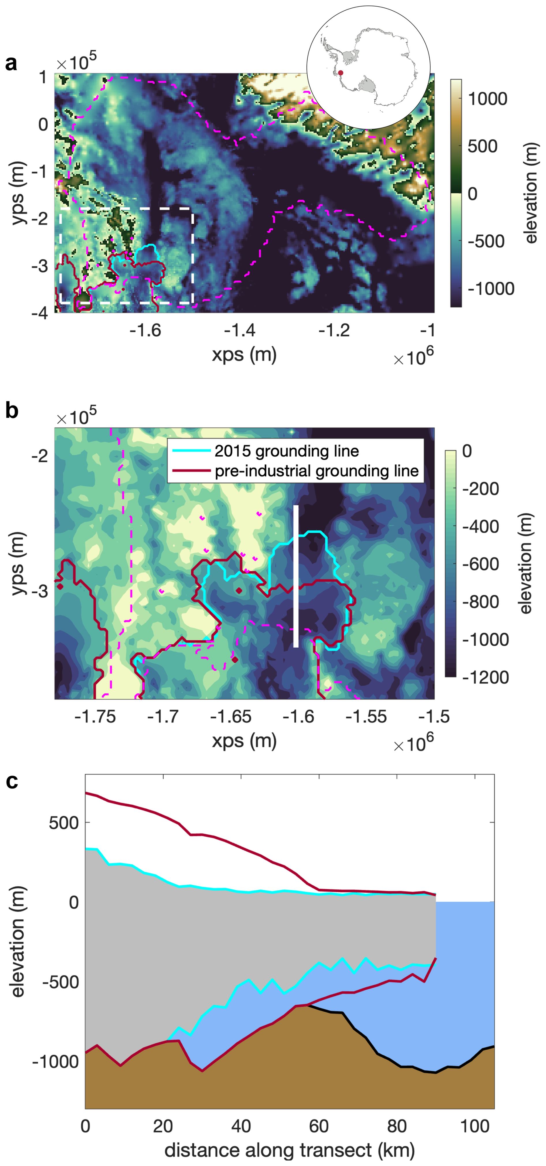
Figure 1 (a) Pine Island Glacier bed elevation (colours) with an outline of the ice mask (pink dashed line). The cyan and red lines indicate the grounding-line position in 2015 and in the initial state (after the cold forcing spin-up), respectively. The inset shows the location of Pine Island Glacier in Antarctica as a red point. xps and yps are co-ordinates in the polar stereographic projection. (b) As in (a), but zoomed in on the Pine Island Ice Shelf (the white dashed box in a). The thick white line indicates the centreline along which the transects in (c) are taken, and along which grounding-line retreat is measured. (c) Along centreline bed topography (shaded brown) alongside ice geometry in 2015 (shaded grey, cyan outline) and in the pre-industrial steady state (red).

The WAVI model comes equipped with a suite of melt rate parametrizations (Bradley et al., 2024a). Here, we apply a quadratic parametrisation of basal melting, where the basal melt rate on floating ice shelves is

$$\begin{array}{}\text{(3)}& \dot{m}=M{T}_{*}^{\mathrm{2}}.\end{array}$$

Here $M=\mathrm{5.0}\times {\mathrm{2}}^{M_{\mathrm{0}}}$ m °C⁻² a⁻¹ is a variable melting calibration coefficient, with M₀ referred to as the melt rate exponent prefactor, and

$$\begin{array}{}\text{(4)}& T_{*}={\mathit{\lambda }}_{\mathrm{1}}{S}_{\mathrm{a}}+{\mathit{\lambda }}_{\mathrm{2}}+{\mathit{\lambda }}_{\mathrm{3}}{z}_{\mathrm{b}}-T_{\mathrm{a}}\end{array}$$

is the local thermal forcing on the ice shelf. T_a and S_a are, respectively, the local ambient temperature and salinity (see Sect. 2.1.3) and z_b is the basal elevation. Here, ${\mathit{\lambda }}_{\mathrm{1}}=\mathrm{5.73}\times {\mathrm{10}}^{-\mathrm{2}}$ °C is the liquidus slope with salinity, ${\mathit{\lambda }}_{\mathrm{2}}=\mathrm{8.32}\times {\mathrm{10}}^{-\mathrm{4}}$ is the freezing temperature offset, and ${\mathit{\lambda }}_{\mathrm{3}}=\mathrm{7.61}\times {\mathrm{10}}^{-\mathrm{4}}$ °C m⁻¹ is the liquidus slope with depth. The melt rate (Eq. 3) is applied everywhere on floating ice shelves, which have a fixed ice front, indicated in Fig. 1b. This ice front position is equal to the 2025 ice front position.

We apply a temporally constant surface accumulation field from Arthern et al. (2006) across our domain, set to present day values.

We simulate the retreat of the PIG on a numerical grid with 3 km resolution. This resolution is chosen as a balance between retaining accuracy and permitting large ensembles of simulations to be run. Recent work (Williams et al., 2025) has shown that numerical simulations are not overly sensitive to resolution in WAVI, provided they are at or below 3 km.

In all simulations, we use a fixed time-step of 0.05 years. However, the Courant-Friedrichs-Levy (CFL) condition, which determines numerical stability, is model parameter dependent. When model parameters are varied in the EKI procedure, we therefore occasionally encounter numerical instabilities. These instabilities manifest as “stripy” ice velocities and thicknesses, particularly in the fast flowing regions of the Pine Island Ice Shelf. Comparison with simulations in which the timestep is reduced reveal that, despite this, modelled ice volume change and grounding-line retreat (which we use as observational constraints on our model – see Sect. 2.2.2) are not affected by this. In addition, simulations which violate the CFL condition are typically associated with rapid retreat (e.g. they correspond to very low basal friction), much faster than observations suggest. These simulations have poor agreement with observations and therefore do not contribute significantly to model parameter estimation.

2.1.2 Initial state

To simulate the evolution of PIG over the industrial era, we need to specify the ice sheet geometry at the start of the simulation. Since this is prior to the satellite era, we do not have observational constraints on ice sheet geometry. Therefore, to obtain a “pre-industrial” state, we follow Reed et al. (2024a): we first take the present day PIG state (Fig. 1a–b) and advance the grounding line to the seabed ridge on which it was grounded prior to the 1940s. This is achieved by turning melting off entirely and timestepping the model forwards for 500 years. After this time, the ice sheet is stably grounded on the ridge with a constant grounding-line position and ice volume. In this configuration, the grounding-line position is consistent with sediment records (Smith et al., 2017), but the ice shelf is too large (Fig. 1c): we do not have observational constraints on the ice geometry prior to the satellite era, but at least some ice shelf basal melting must have been taking place. To address this, we run a spin-up period in which melting is turned on, with M₀=0, and cold ocean forcing conditions (corresponding to the coldest observed conditions, defined formally in Sect. 2.1.3) applied. With M₀=0, basal melt rates in the present day geometry yield total freshwater fluxes that closely match observations (Dutrieux et al., 2014). This spin-up period lasts 50 years; during this time, the grounding line retreats slightly, but remains grounded on the ridge.

The ice geometry after the spin-up is considered to be the pre-industrial state, and is referred to as the initial state. All results presented here are conditional on this choice. In our framework, this state is not a true steady state for each simulation because we vary the model parameters at the start of the simulation (see Sect. 2.1.3) and the ice will respond to this perturbation. The time that this takes depends on the specific model parameter perturbation; it is hard to assess a priori, as the CES procedure itself selects model parameter values which are compatible with observations. For the prior-mean parameter combinations, this response time is small (years), but, as we shall see, for some model and climate forcing parameter the CES procedure nudges parameter distributions some way from the priors.

Each of our simulations begins in 1750, using the same initial state. Ideally, we would run our simulations for longer, by setting the initial state to correspond to further back in time, allowing memory of the initial state to be lost and removing the effect of the initialisation shock. However, this incurs an additional computational expense, and 1750 is chosen as a balance between extra computational expense and attempting to run for long enough to minimise initial state dependence. We discuss the implications of this choice in Sect. 4.

2.1.3 Climate Forcing and Parameters

Following the spin-up, variable climate forcing is applied to the ice sheet via the ambient ocean temperature (T_a) and salinity (S_a) in the melt rate parametrization (Eq. 3). We take ambient temperature and salinity profiles which are similar to observations (De Rydt et al., 2014; Dutrieux et al., 2014). These profiles are piecewise linear: they are constant in both an upper (temperature −1 °C, salinity 34 PSU, corresponding to Winter Water) and lower layer (temperature 1.2 °C, salinity 34.7 PSU, corresponding to Circumpolar Deep Water), which are separated by a pycnocline of 400 m thickness, across which the temperature and salinity vary linearly (Fig. 2a–b). Ocean variability and trends in the Amundsen Sea are primarily manifested as a thickening or thinning of the deep Circumpolar Deep Water layer, rather than substantial variation in the temperature or salinity of the upper or lower layers (Dutrieux et al., 2014; Naughten et al., 2023). Therefore we impose all climatic variability by raising and lowering the pycnocline, and so the depth of the centre of the pycnocline, denoted P_c, parameterizes the entire ambient temperature and salinity profile.

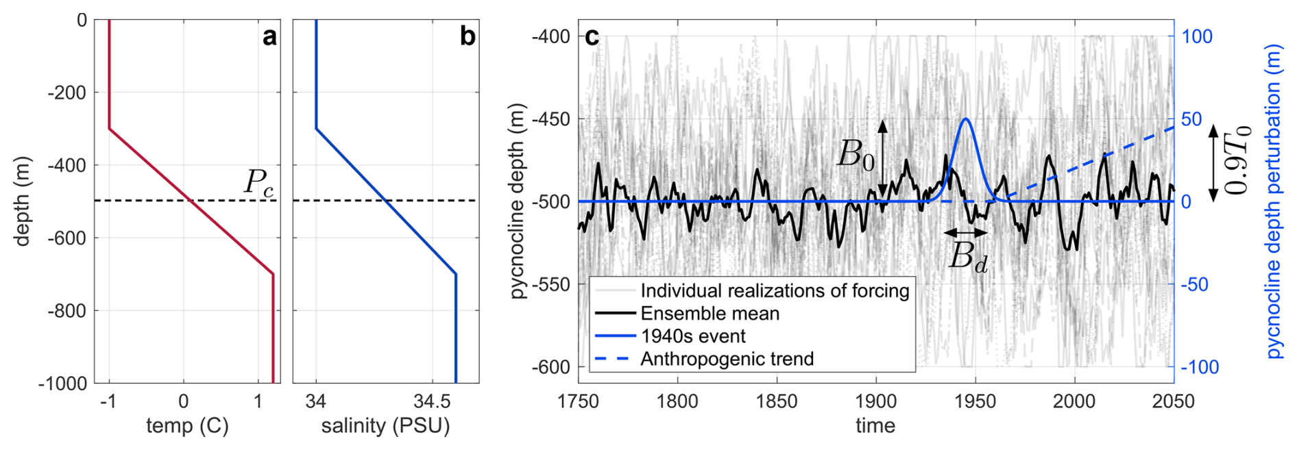
Figure 2 Example ambient temperature (a) and salinity profiles (b) used in the melt rate parameterization (Eqs. 3–4). The pycnocline is displaced up and down to represent climatic variability, with no change in upper or lower layer properties, so the depth of the pycnocline centre, P_c, parametrizes the profiles. In the examples shown here, $P_{\mathrm{c}}=-\mathrm{500}$ m. (c) Components of the forcing (Eq. 5). Translucent black curves indicate individual realizations of internal variability, $P_{\mathrm{c},\mathrm{0}}+\mathit{\alpha }R\left(t\right)$, and the solid black curve indicates the ensemble mean of these. Also shown (corresponding to the right-hand axis) are the 1940s event perturbation to the forcing, B(t) (solid blue), and anthropogenic trend, T(t) (dashed blue). In this case, we show B_d=5 years, B₀=50 m, T₀=50 m (0.9T₀ is indicated because the centennial trend is initiated in 1960 and plotted until 2050, i.e. 90 years).

The temporally varying pycnocline centre depth encodes information about climate forcing. It is expressed as term corresponding to internal variability super-imposed on terms corresponding to the 1940s event and anthropogenic trends in forcing, with the latter two representing the theorised leading order controls on retreat over the industrial era. These are encoded by setting the pycnocline centre as (Fig. 2c):

$$\begin{array}{}\text{(5)}& P_{\mathrm{c}}\left(t\right)=P_{\mathrm{c},\mathrm{0}}+\mathit{\alpha }{\displaystyle \frac{R\left(t\right)}{\mathrm{4}}}+B\left(t\right)+T\left(t\right)\end{array}$$

Here, $P_{\mathrm{c},\mathrm{0}}=-\mathrm{500}$ m is a typical observed pycnocline depth (Webber et al., 2017). Below, we describe each of these components in detail.

The second term on the right hand side of Eq. (5) corresponds to internal variability other than the 1940s event (see below). The shallowest and deepest observed pycnocline depths are approximately −400 and −600 m, respectively (Dutrieux et al., 2014) and thus the parameter α=200 m is the magnitude of differences between warmest and coldest conditions associated with internal variability. R(t) is a dimensionless timeseries generated from a modified first-order autoregressive process: it is as in Christian et al. (2022) and Bradley et al. (2024b), with interdecadal-to-decadal timescales well represented, but is truncated between −2 and 2 (so α is four times the standard deviation of this autoregressive process). Noise in the autoregressive process has a Gaussian distribution. We take a decorrelation timescale of 10 years in the autoregressive process, which ensures that it captures decadal variability (Jenkins et al., 2018). Note that this formulation of forcing assumes that the pre-industrial pycnocline centre and amplitude is equivalent to present day pycnocline centre and amplitude, respectively; this is consistent with an assumption of zero anthropogenic trend in forcing, which we take as the prior value on this quantity (see Sect. 2.2.1).

In the spin-up period described in the previous section, the pycnocline centre is set to a constant value of −600 m. This is to ensure that ice sheet is in a pseudo-steady state after the spin-up period, for those parameters used for the spin up. When the stochastic forcing (Eq. 5) is turned on, the mean pycnocline centre becomes −500 m. The ice sheet will respond to this perturbation at the start of the simulation (in addition to responding to the changes in ice sheet model parameters, including those that relate to ice shelf melting, that take place at the same time).

To facilitate a quantification of aleatoric uncertainty (uncertainty associated with the chaotic forcing), we repeat the CES procedure outlined in the following section for multiple realizations of the autoregressive process, which we refer to as realizations of forcing. In total, we consider 14 individual realizations of forcing, shown in Fig. 2c. The ensemble mean of the autoregressive internal variability components is close to, but not zero (Fig. 2c), owing to the finite size of the ensemble of different realizations.

The purely random internal variability component does not capture the anomalously strong 1940s event in the ensemble mean (Fig. 2c). To probe the effect of the 1940s event in 20th century PIG retreat, we therefore explicitly superimpose a term capturing the effect of this event in the internal variability. This is imposed by setting

$$\begin{array}{}\text{(6)}& B\left(t\right)=B_{\mathrm{0}}\text{exp}\left[-{\displaystyle \frac{(t-\mathrm{1945}{)}^{\mathrm{2}}}{\mathrm{2}{B}_{\mathrm{d}}^{\mathrm{2}}}}\right],\end{array}$$

where B₀ is the magnitude of the 1940s pycnocline displacement (away from the internal variability component) in metres and B_d is its duration (Fig. 2c). B₀ and B_d are variable parameters, whose posterior distributions are inferred using the CES procedure, i.e. our parameter inference provides estimates of how long and how large the 1940s event was in terms of its effect on the pycnocline position. It is important to stress that the 1940s event is technically part of the internal variability, viewed as independent of anthropogenic influence. We choose to impose it in this deterministic (rather than stochastic) way to enable us to quantify its effect on 20th century PIG retreat.

The final component of the pycnocline position Eq. (5) is the anthropogenic trend in forcing,

$$\begin{array}{}\text{(7)}& T\left(t\right)=T_{\mathrm{0}}\left({\displaystyle \frac{t-\mathrm{1960}}{\mathrm{100}}}\right)\times H(t-\mathrm{1960}),\end{array}$$

where T₀ is the per-century-trend in pycnocline height in metres, and H(ξ) is the Heaviside function, taking the value of one for ξ≥0 and zero for ξ<0 (in particular, this means that the anthropogenic trend in forcing continues indefinitely). T₀ is considered a variable parameter, to be inferred from the CES procedure; in making inference into this parameter, we are addressing the question: how large does the anthropogenic trend in forcing have to have been to explain the PIG retreat that has occurred over the industrial era? Note that in setting the trend according to Eq. (7), we assume that the trend begins in the 1960s and is linear, which is consistent with trends in shelf-break winds (Holland et al., 2019, 2022).

2.2 Observationally-constrained posterior parameter distributions using CES

We aim to produce observationally constrained posterior distributions of the set of model and climate parameters, $\mathrm{\Theta }=(A_{\mathrm{0}},C_{\mathrm{0}},M_{\mathrm{0}},B_{\mathrm{0}},B_{\mathrm{d}},T_{\mathrm{0}})$. To do so, we follow the calibrate, emulate, sample procedure outlined in Cleary et al. (2021). In this section, we describe each of these steps in detail, as well as the observations used as constraints. For each of the 14 realizations of internal variability in the forcing from the autoregressive process, we produce a unique posterior distribution of the parameters. Samples from these posterior distributions are then taken and run over the industrial period (see Sect. 3) to reconstruct the behaviour of PIG since 1750 and facilitate an attribution assessment.

The steps of the CES procedure are as follows: in the first step (calibrate), an adaptive procedure (here, EKI) is used to obtain parameter samples that minimise model–observation error. Having many samples in the “likely” region of parameter space, where the model–observation error is small, ensures that the emulator constructed in the following step (emulate) is accurate, with low uncertainty, for parameters in this region. This emulator gives statistical approximations to the model output, and thus model–observation error, everywhere in parameter space. In the final step (sample), Markov-chain Monte Carlo sampling is used to generate posterior distributions of model and climate parameters, with step updates in the Markov-chain based on the approximate model–observation error constructed in the emulate step.

2.2.1 Prior distributions of model and climate parameters

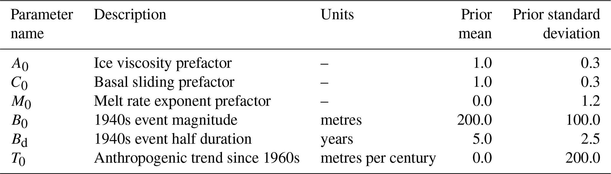
Prior distributions of model parameters (i.e. before observations have been assimilated) are assumed to be all Gaussian, with mean and standard deviation as shown in Table 1. The prior mean on the basal melt rate exponent prefactor (M₀=0) results in a melt rate parametrization $\dot{m}=\mathrm{5.0}{T}_{*}^{\mathrm{2}}$; as mentioned, this choice ensures that the basal melt flux in the present day with warm ambient conditions ($P_{\mathrm{c}}=-\mathrm{400}$ m) matches the basal melt flux with corresponding conditions in 2009, the warmest year on record (Dutrieux et al., 2014). We assume relatively broad priors on model and climate forcing parameters, indicating little prior knowledge about their likely values. Crucially, we assume that the prior mean on the anthropogenic trend in forcing is zero, so as not to precondition the procedure to select an anthropogenic trend.

Table 1 Descriptions of the model and climate parameters and values of their prior means and standard deviations.

2.2.2 Observations used in the CES procedure

Posterior distributions of model and climate parameters are determined by assimilating observations of ice sheet behaviour. Here, we use observations of grounding-line position in 1930 and 2015, and the volume of grounded ice in 2015. The grounding-line position is measured along the centreline indicated in Fig. 1, and is determined as the weighted average of the positions of the first partially grounded cell and the last full floating cell (measured in the direction into the grounded ice), with the grounded fraction of a grid cell determined using the procedure outlined in Seroussi and Morlighem (2018). The 1930 grounding-line position is taken as that from the initial state geometry, i.e. before any retreat has been initiated. The 2015 grounding-line position and grounded volume are computed from the model ice sheet state following the inversion with present-day observations. In the following, we express the grounding-line position as a grounding-line retreat, measured relative to the 1930 grounding-line position. We assume that both observations of grounding-line position are relatively poorly constrained, taking the observational errors in these quantities to be 3 km, equivalent to one grid cell. The observational error on the 2015 grounded volume is taken to be 10¹² m³. This is a conservative order of magnitude estimate (0.2 % of the ice volume in the initial state), based on errors in mass balance estimates from Otosaka et al. (2023), which are on the order of millimetres of sea level rise, while PIG contains order meters of sea level rise potential. For simplicity, we assume that the observational errors are uncorrelated.

2.2.3 Calibrate

In the calibrate step of the procedure, we use an ensemble Kalman inversion, which is an iterative procedure in which the set of simulated model parameters is updated step-by-step so that model outputs are nudged progressively closer to observations. In simple terms, there are four main substeps within the calibrate step: firstly, an ensemble of parameter samples are chosen and, for each, the model is run and we calculate how close its prediction is to the real observations. Then, we calculate the overall pattern of how far off the simulated values from these parameter samples are from the observations, which informs the direction in which the parameter samples need to move. Next, based on these errors and how sensitive the model is to changes in the parameters, the parameters are nudged, with each guess moving in the direction that reduces the error. Finally, the model is run again with these updated guesses and the update step is repeated until the model predictions are close enough to the observations.

In more detail, the EKI is initialized by sampling J times from the prior distribution of model parameters, giving a set of parameter values ${\mathrm{\Theta }}_{\mathrm{0}}^{\mathrm{1}},\mathrm{\dots },{\mathrm{\Theta }}_{\mathrm{0}}^J$, where the “0” subscript refers to this being the zeroth iteration (in this section, we use subscripts to denote the iteration number and superscripts to denote the samples within this iteration).

After the ith iteration, the jth sample is updated with an update step (second term on the right hand side below) to (Cleary et al., 2021; Bach and Dunbar, 2023)

$$\begin{array}{}\text{(8)}& {\mathrm{\Theta }}_{i+\mathrm{1}}^j={\mathrm{\Theta }}_i^j+C_i^{\mathrm{\Theta }\mathcal{G}}{\left(\mathrm{\Gamma }+C_i^{\mathcal{G}\mathcal{G}}\right)}^{-\mathrm{1}}\left[y-\mathcal{G}\left({\mathrm{\Theta }}_i^j\right)\right].\end{array}$$

The update step is expressed as the product of a step size, $C_i^{\mathrm{\Theta }\mathcal{G}}{\left(\mathrm{\Gamma }+C_i^{\mathcal{G}\mathcal{G}}\right)}^{-\mathrm{1}}$, and a model-observation error, $y-\mathcal{G}\left({\mathrm{\Theta }}_i^j\right)$. In the model–observation error term, y are the observations (i.e. an array containing the grounding-line position in 1930 and 2015, and the ice volume in 2015) and Γ is the error in the these observations. $\mathcal{G}\left({\mathrm{\Theta }}_i^j\right)$ are the modelled values corresponding to the observations, i.e. the simulator (the ice sheet model) 𝒢 evaluated at parameter values ${\mathrm{\Theta }}_i^j$.

In the step size, we have

$$\begin{array}{}\text{(9)}& C_i^{\mathrm{\Theta }\mathcal{G}}={\displaystyle \frac{\mathrm{1}}{J}}\sum _{j=\mathrm{1}}^n\left[\left({\mathrm{\Theta }}_i^j-{\stackrel{\mathrm{‾}}{\mathrm{\Theta }}}_i\right){\left(\mathcal{G}\left({\mathrm{\Theta }}_i^j\right)-{\stackrel{\mathrm{‾}}{\mathcal{G}}}_i\left(\mathrm{\Theta }\right)\right)}^T\right],\end{array}$$

which plays the role of a cross-covariance between parameters Θ and model outputs 𝒢(Θ), encoding how changes in the model parameters relate to changes in the model predictions. Here, the overbar denotes an average over the ensemble members at this iteration. In Eq. (8), we also have

$$\begin{array}{}\text{(10)}& C_i^{\mathcal{G}\mathcal{G}}={\displaystyle \frac{\mathrm{1}}{J}}\sum _{j=\mathrm{1}}^J\left[\left(\mathcal{G}\left({\mathrm{\Theta }}_i^j\right)-{\stackrel{\mathrm{‾}}{\mathcal{G}}}_i\left(\mathrm{\Theta }\right)\right){\left(\mathcal{G}\left({\mathrm{\Theta }}_i^j\right)-\stackrel{\mathrm{‾}}{\mathcal{G}}\left({\mathrm{\Theta }}_i\right)\right)}^T\right],\end{array}$$

which plays the role of the output covariance of 𝒢(Θ), encoding how much the model outputs vary together across the ensemble.

In the results generated in this study, we use J=20 ensemble members and five iterations, giving 100 simulations for each realization of forcing. The total number of simulations is thus 1400=20 ensemble members ×5 iterations ×14 realizations of forcing. There is no general rule on how many ensemble members and iterations should be used in an EKI. However, we found that with fewer ensemble members (J=10), parameter updates (Eq. 8) would be swamped by some ensemble members with large model–observation errors, which drives the whole ensemble away from the optimal parameter values. Other studies (e.g. Cleary et al., 2021; Mansfield and Sheshadri, 2022), with different model operators 𝒢, have found that smaller J yields good convergence.

Figure 3a–b demonstrate how trajectories of grounded ice volume and grounding-line retreat converge as iterations proceed, indicating the potential of the EKI to obtain trajectories of ice sheet change which are consistent with observed changes. Corresponding parameter values are shown in Fig. 3c–h. Parameter values do not converge to a single value, but towards a distribution, which are approximate samples from the posterior of the parameters (Cleary et al., 2021).

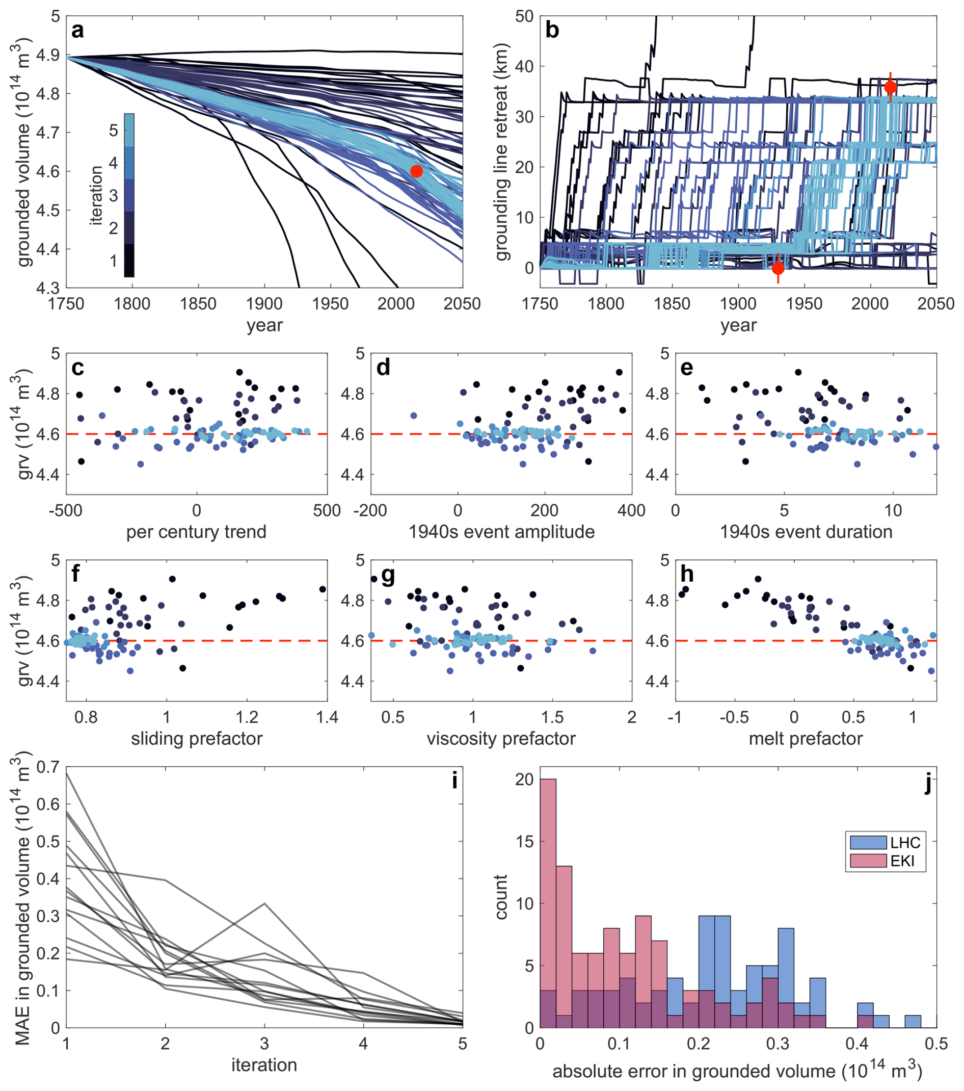
Figure 3 (a–b) Trajectories of (a) grounded volume and (b) grounding-line retreat in simulations of Pine Island Glacier. Colours correspond to the different iterations, as indicated by the colour bar in (a). Results are shown for a single realization of forcing. Red points indicate observational constraints used on trajectories in the EKI, with error bars indicating uncertainties in observations (note that the error bar does not extend beyond the point in a). (c–h) Scatter plots of grounded ice volume (grv) in 2015 as a function of (c–e) climate and (f–h) model parameters for simulations whose trajectories are shown in (a)–(b) (and are therefore only for a single realization of forcing). Colours of points correspond to iterations as indicated in (a). In each panel, the red dashed line indicates the observational constraint. (i) Mean (over ensemble members) absolute error in the grounded volume as a function of iteration number. Results are shown for all 14 realizations of forcing. (j) Histograms of absolute errors in the grounded volume obtained from the EKI (red) and a Latin hypercube sampling method (blue), for a single realization of forcing. In both cases, the ensemble consists of 100 simulations.

We find that in each realization of forcing, by the fifth iteration the mean absolute error – the mean (over the ensemble members) of the model–observation error – in the grounded volume is below 0.05×10¹⁴ m³ (approximately 1 % of the total ice volume, see Fig. 3i).

It is interesting to compare the outcomes of the EKI procedure with those from Latin hypercube sampling (Fig. 3j), the current standard sampling method in ice sheet modelling. Latin hypercube sampling ensures that the parameter space is evenly covered, usually by applying a space-filling algorithm which ensures that the distance between points is maximised. To generate a Latin hypercube sample, a fixed range of parameters must be specified; for the comparison here, we set these limits to be two standard deviations either side of the mean of the prior distributions. Histograms of errors in the grounded volume (Fig. 3j) confirm that the errors in the EKI ensemble (based on all iterations of the EKI) are significantly smaller than those in the LHC ensemble: for this particular problem, EKI sampling is superior to LHC sampling when assessed in terms of observational constraints. Additionally, errors in the final iteration of the EKI (left most bin of Fig. 3j) are small and considerably lower than the average from the LHC.

2.2.4 Emulate

In the next step, we train emulators (computationally cheap statistical approximations of the expensive simulator) on the calibrated simulations described in the previous section. Essentially, the emulators are cheap models, based on the expensive simulations, which approximate the model's prediction of the three observational values. Doing so allows us to evaluate the model output, and thus construct model–observation errors, for any parameter values (i.e. not just those sampled with model simulations during the calibration step). This model–observation error is used in the Markov chain Monte Carlo (MCMC) sampling, described in the following section.

In more detail, the simulator can be considered a map M_s between input parameters Θ and predictions of the quantities for which we have observations, i.e.

$$\begin{array}{}\text{(11)}& \begin{array}{rl}{M}_{\mathrm{s}}\left(\mathrm{\Theta }\right)=& \left(\mathrm{1930}\text{grounding-line position},\right.\\ & \mathrm{2015}\text{grounding-line position},\\ & \left.\mathrm{2015}\text{grounded ice volume}\right).\end{array}\end{array}$$

The emulators are approximations to the map M_s. We construct emulators for each of the observational constraints individually, giving maps $M_{\mathrm{e}}^{\mathrm{1}}\left(\mathrm{\Theta }\right),M_{\mathrm{e}}^{\mathrm{2}}\left(\mathrm{\Theta }\right),M_{\mathrm{e}}^{\mathrm{3}}\left(\mathrm{\Theta }\right)$ where

$$\begin{array}{}\text{(12)}& \begin{array}{rl}& (\text{1930 grounding line, 2015 grounding line,}\\ & \text{2015 grounded ice volume})\\ & =M_{\mathrm{s}}\left(\mathrm{\Theta }\right)\approx \left(M_{\mathrm{e}}^{\mathrm{1}}\right(\mathrm{\Theta }),M_{\mathrm{e}}^{\mathrm{2}}(\mathrm{\Theta }),M_{\mathrm{e}}^{\mathrm{3}}(\mathrm{\Theta }\left)\right).\end{array}\end{array}$$

Importantly, the functions $M_{\mathrm{e}}^{\mathrm{1}}\left(\mathrm{\Theta }\right),M_{\mathrm{e}}^{\mathrm{2}}\left(\mathrm{\Theta }\right),M_{\mathrm{e}}^{\mathrm{3}}\left(\mathrm{\Theta }\right)$ can be evaluated everywhere in parameter space, whereas the map M_s(Θ) is only known at discrete values where the simulations exist. The emulators match the simulated values for each point in the parameter space where there is a simulation, and provide predictions for all other points in the parameter space, alongside an estimate of uncertainty in this prediction.

This process is repeated for each realization of forcing, giving $\mathrm{14}\times \mathrm{3}=\mathrm{42}$ emulators in total. Each emulator is a Gaussian process – a non-parametric method that treats the simulator as an unknown function of its inputs (O’Hagan, 2006). For a given set of inputs, a Gaussian process returns a Gaussian distribution of outputs, which is characterised by its mean and standard deviation. The mean and standard deviation can be considered the emulator's central estimate of the model output and its uncertainty in this prediction, respectively, for these parameter values. Importantly, the Gaussian processes provides uncertainty estimates, which are not directly available in many other emulation methods, such as neural networks (Gawlikowski et al., 2023). These uncertainty estimates are propagated through the MCMC sampling to ensure that emulator error is robustly represented in posterior distributions of model and climate parameters. We train the emulators on all the simulations from the EKI, rather than following the suggestion of Cleary et al. (2021) and only use those simulations from the final iteration, as this was found to improve emulator performance, i.e. the ability of the emulators to reproduce the simulated model output. This is likely because using all iterations means that the training data set (the set of simulated model outputs and corresponding input parameters Θ) is larger.

To construct the emulators, we use the R package RobustGaSP (Gu et al., 2019). Each emulator uses a Matérn 3/2 kernel, which we found displayed the best coverage (the percentage of emulator predictions of model output that are more than two emulator standard deviations away from corresponding model output), and lowest RMSE of five standard kernel choices: Matérn (3/2), Matérn (5/2), and three members of the power exponential family with high, medium, and low exponent values (α=1.9, α=1.0, and α=0.1) in a leave-one-out-cross-validation experiment (Bastos and O’Hagan, 2009), which is described in the next paragraph.

To validate our emulators, we perform a leave-one-out-cross-validation. In this procedure, each emulator is sequentially trained on the output of every set of parameter values used in the EKI except for one (i.e. on 99 parameter sets), and then evaluated on the remaining parameter set. For each, we note the emulator prediction and uncertainty in the prediction. We use the coverage as a metric for emulator performance (Fig. 4a). We find that most emulators have coverages between 80 % and 90 % (mean 85 %, 87 %, and 91 % standard deviation 3 %, 4 %, and 3 % for 2015 grounded ice volume, 1930 grounding-line retreat and 2015 grounding-line retreat, respectively), reflecting good performance. In addition, many of the data points outside the two emulator standard deviation bands have low root mean squared error.

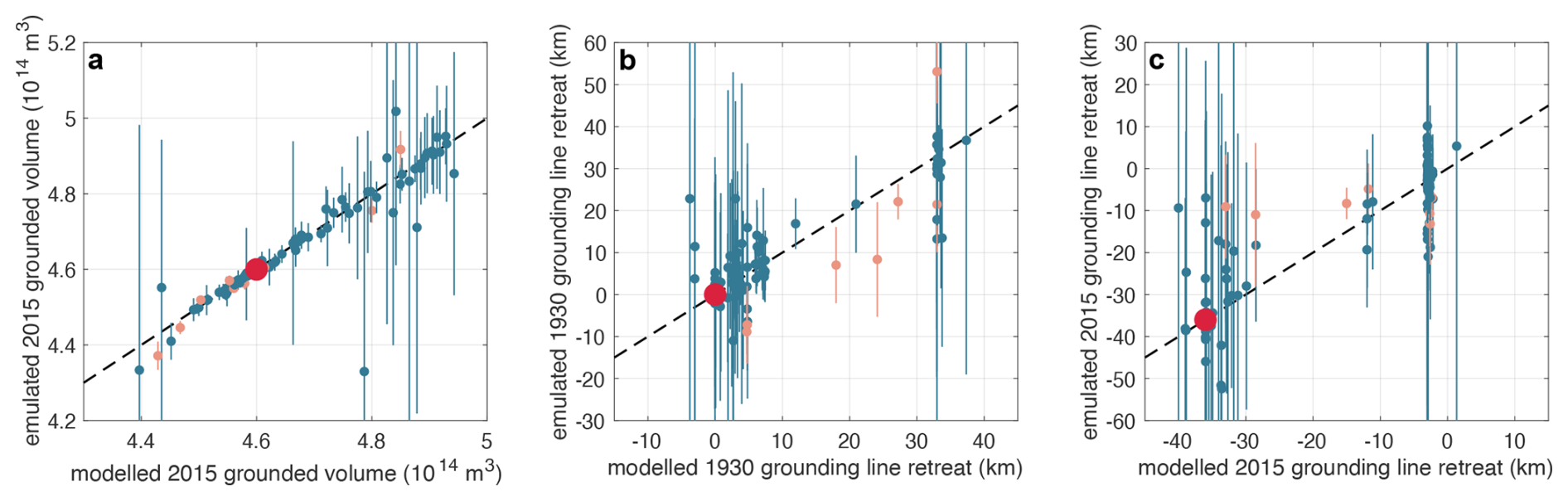
Figure 4 Results of a leave-one-out-cross validation of model emulators. Each panel contains a scatter plot of modelled versus emulated quantities, as follows: (a) 2015 grounded ice volume, (b) 1930 grounding-line retreat relative to the pre-industrial position and (c) 2015 grounding-line retreat relative to the pre-industrial position. In each case, blue (orange, respectively) markers are used for simulations in which the emulated quantity is inside (outside) one emulator standard deviation of the modelled value. Error bars indicate the standard deviation of each emulator prediction. Black dashed lines are 1–1 lines, onto which each point would fall if the emulated values perfectly matched the modelled values. Results are shown for a single realization of forcing.

2.2.5 Sample

Having emulated model predictions of observational constraints, we construct posterior distributions of model and climate parameters using MCMC sampling. The sampling step uses the fast emulator to explore a wide range of possible inputs quickly, generating many outputs. This allows us to determine which parameter values are likely (and which aren't) based on agreement between outputs and observations, without having to run the slow, full simulation repeatedly.

The Markov chains move through the space of model and climate parameters Θ. Each is initialized with parameter values that are the mean of the final iteration of the EKI: writing Φ_n for the state of the Markov Chain at its nth step, we take ${\mathrm{\Phi }}_{\mathrm{0}}={\stackrel{\mathrm{‾}}{\mathrm{\Theta }}}_{\mathrm{5}}$. Following Cleary et al. (2021), we use a Metropolis-Hastings algorithm for the update step of the Markov chain. The size of this update step in this algorithm is determined from a multivariate Gaussian distribution whose covariance is given by the empirical covariance of the ensemble from the EKI – essentially the spread and relationship of the previous samples from the EKI (see below). These choices of initial state and update step size pre-condition the Markov chain with approximate information about the posterior distribution of model and climate parameters from the EKI, allowing the MCMC to be initialized into a state close to the posterior mean (Cleary et al., 2021).

Explicitly, the MCMC algorithm is as follows (see italic text at the start of each step for a non-mathematical explanation):

1. Start the procedure with the parameters corresponding to the end of the EKI procedure.
   Initiate the MCMC with parameter values ${\mathrm{\Phi }}_{\mathrm{0}}={\stackrel{\mathrm{‾}}{\mathrm{\Theta }}}_{\mathrm{5}}$.

2. To make a step, suggest new values of the parameters. The size of this step depends on the spread and relationship of the samples from the EKI.
   At the kth step in the chain, propose a new Markov chain state ${\mathrm{\Phi }}_{k+\mathrm{1}}^{*}={\mathrm{\Phi }}_k+{\mathit{\zeta }}_k$ where

   $$\begin{array}{}\text{(13)}& {\mathit{\zeta }}_k\sim \mathcal{N}\left(\mathrm{0},{\displaystyle \frac{\mathrm{1}}{J}}\sum _{j=\mathrm{1}}^J\left[\left({\mathrm{\Theta }}_{\mathrm{5}}^J-\stackrel{\mathrm{‾}}{\mathrm{\Theta }}\right)\otimes \left({\mathrm{\Theta }}_{\mathrm{5}}^J-\stackrel{\mathrm{‾}}{\mathrm{\Theta }}\right)\right]\right),\end{array}$$

   with 𝒩 denoting a normal distribution and ⊗ is the tensor product.

3. Calculate the relative likelihood of the previous and proposed parameters. These likelihoods are based on how well the corresponding emulator outputs (i.e. the emulator output for the current and proposed parameters) agree with observations, as well as the prior likelihood of these parameters (i.e. before any data assimilation), and how uncertain the emulator is for these parameters. Lower likelihoods are obtained for parameter sets which: have higher emulator-observation error; have less likely prior; and for which the emulator is more uncertain.
   Compute the acceptance probability $a({\mathrm{\Phi }}_k,{\mathrm{\Phi }}_{k+\mathrm{1}}^{*})$ where

   $$\begin{array}{}\text{(14)}& \begin{array}{rl}a(s,t)& =\text{min}\left\{\mathrm{1},\text{exp}\left[\left({\mathrm{\Psi }}^M\left(s\right)+{\displaystyle \frac{\mathrm{1}}{\mathrm{2}}}\left|\right|s|{|}_{{\mathrm{\Gamma }}_{\mathrm{\Theta }}}^{\mathrm{2}}\right)\right.\right.\\ & -\left.\left.\left({\mathrm{\Psi }}^M\left(t\right)+{\displaystyle \frac{\mathrm{1}}{\mathrm{2}}}\left|\right|t|{|}_{{\mathrm{\Gamma }}_{\mathrm{\Theta }}}^{\mathrm{2}}\right)\right]\right\}\end{array}\end{array}$$

   where

   $$\begin{array}{}\text{(15)}& \begin{array}{rl}{\mathrm{\Psi }}^M\left(\mathrm{\Theta }\right)& ={\displaystyle \frac{\mathrm{1}}{\mathrm{2}}}{\left(\left|\right|y-\mathcal{G}\left(\mathrm{\Theta }\right)|{|}_{{\mathrm{\Gamma }}_{\mathrm{GP}}+{\mathrm{\Gamma }}_y}\right)}^{\mathrm{2}}\\ & +{\displaystyle \frac{\mathrm{1}}{\mathrm{2}}}\text{log}\left\{\text{det}\left[{\mathrm{\Gamma }}_{\mathrm{GP}}\left(\mathrm{\Theta }\right)+{\mathrm{\Gamma }}_y\right]\right\},\end{array}\end{array}$$

   with $\left|\right|a|{|}_A=|\left|A^{-\mathrm{1}/\mathrm{2}}a\right||$ for any positive-definite matrix A and $\left|\right|.\left|\right|$ denoting the L2-norm. Γ_GP(Θ) is the (parameter dependent) covariance matrix of the emulators. Γ_y is the covariance matrix of the observations. Γ_Θ is the covariance matrix of the prior distribution of model and climate forcing parameters Θ.

4. Decide whether to move to the proposed parameters based on the likelihood calculated in the previous step.
   Update the chain to Φ_k+1 to ${\mathrm{\Phi }}_{k+\mathrm{1}}^{*}$ with probability $a({\mathrm{\Phi }}_k,{\mathrm{\Phi }}_{k+\mathrm{1}}^{*})$; otherwise set ${\mathrm{\Phi }}_{k+\mathrm{1}}={\mathrm{\Phi }}_k$.

5. Repeat the previous steps many times to build up a distribution of sampled parameters.
   Repeat steps 2–4 S times. In the results presented here, we use S=50 000.

6. Remove some samples from the start, where the chain has not yet settled into the right area.
   Remove the first S_burn samples from the sequence (the “burn in” period). In the results presented here, we use S_burn=1000.

Samples from the MCMC yield posterior distributions of model and climate parameters. Note that the likelihood Eq. (15) consists of a first term corresponding to the model–observation error and a second term corresponding to uncertainty in both the observations Γ_y and the emulator Γ_GP(Θ), i.e. emulator uncertainty is explicitly accounted for in the posterior distributions of model and climate parameters.

3 Results

3.1 Posterior distributions of climate and model parameters

Posterior distributions of climate and model parameters are shown in Fig. 5. In general, the posterior distributions are much tighter than the priors, indicating that the three observational constraints assimilated during the CES procedure provide strong controls on model and climate forcing parameters. In other words, the region of parameter space which is compatible with the particular retreat of PIG over the 20th century is small, despite our choice to permit fairly broad errors on observational constraints. Although the posterior distributions for each realization of forcing are relatively narrow, the combined posterior distribution (obtained by taking all samples from the 14 individual CES procedures) can remain broad, particularly for the ice viscosity prefactor (Fig. 5b), anthropogenic trend (Fig. 5d), and the 1940s event duration (Fig. 5f). This indicates that aleatoric uncertainty is a major contributor to uncertainties in model and climate parameters. This finding is consistent with previous work (Robel et al., 2019), which has demonstrated that aleatoric uncertainty plays an important role in ice-ocean systems, particularly those which are subject to strong ice-ocean feedbacks. Thus, we re-iterate that ice sheet modelling studies should consider multiple realizations of forcing when making assessments of future and past change. Furthermore, internal variability in the chaotic climate system is unpredictable, so this demonstrates an irreducible source of uncertainty inherent in all ice sheet predictions.

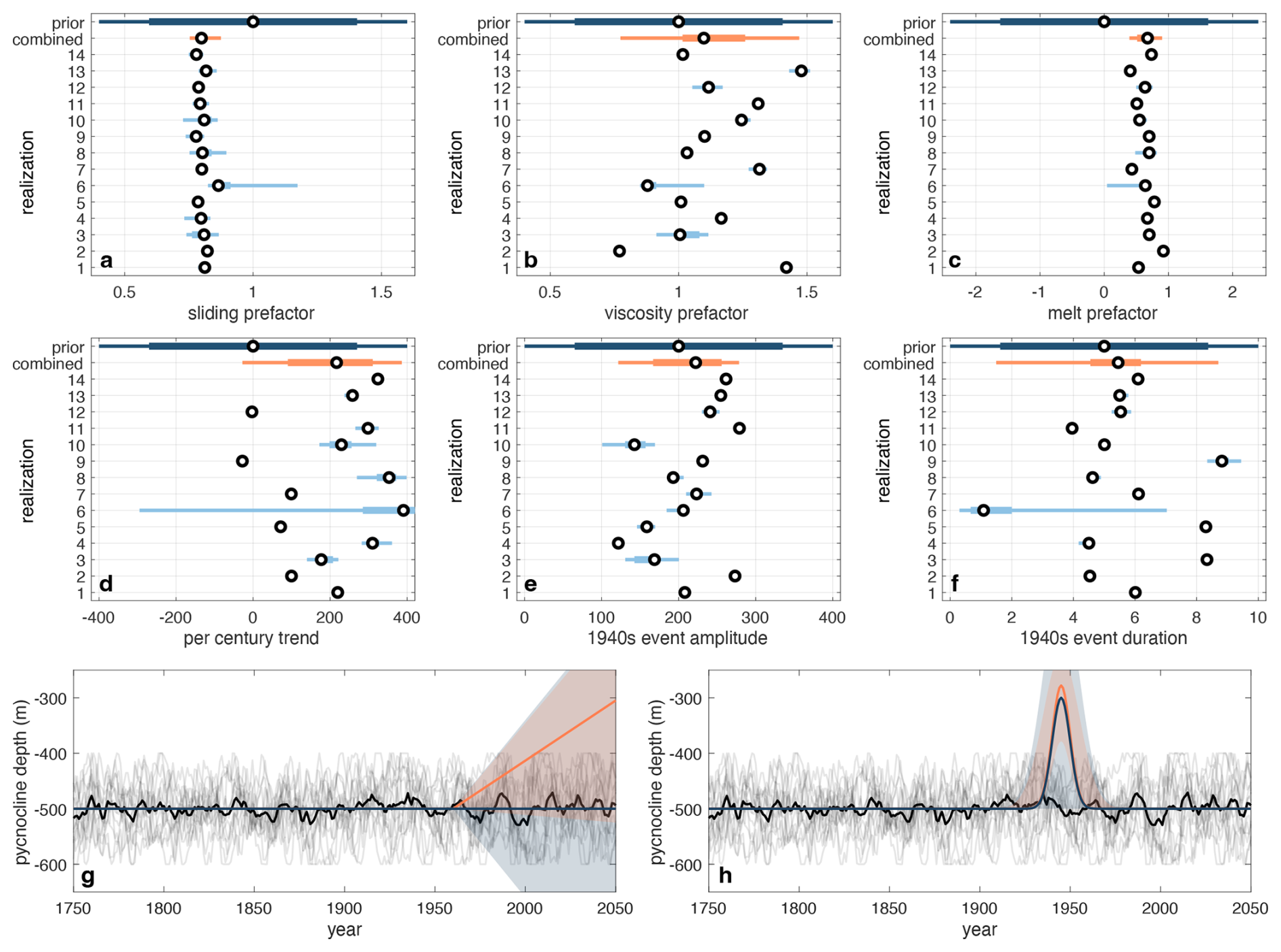
Figure 5 (a–f) Posterior distributions of model and climate parameters. Each panel corresponds to an individual parameter as labelled on the abscissae. Distributions are shown for each realization of forcing (numbered 1–14, light blue), for the combined posterior distribution (orange), and for the prior (dark blue). For each, narrow lines indicate the 95 % interval, thick lines indicate the interquartile range, and black points indicate the median. (g–h) Prior and posterior trajectories of climate forcing. In both panels, contributions to the forcing from the prior and posterior mean (shading: 95 % confidence interval) arising from the anthropogenic trend in forcing (g) and 1940s event (h) are shown in blue and orange, respectively. As in Fig. 2c, the individual realizations of forcing are shown as translucent black curves and the ensemble mean of these is shown as a thick black curve.

Our observationally constrained posterior distributions provide inference into both the past climate as well as the physical model. We find that the posterior distribution on the basal sliding prefactor is tight relative to the prior, (posterior mean: 0.79, 95 % confidence interval: [0.75, 0.87], while the prior has a 95 % confidence interval of [0.412, 1.588]). This indicates that the field of basal sliding coefficients should be adjusted by approximately 20 % to correctly capture the evolution of the Pine Island Glacier over the 20th century, within the context of the other parameters varied and model structure (see below).

Similarly, the posterior distribution on the melt rate exponent prefactor has mean 0.67 (95 % confidence interval: [0.39, 0.9]), indicating that the melt rate is significantly higher (by a factor of 1.59, 95 % confidence interval: [1.31, 1.87]) than the prior. Recall that the prior is constrained by observations: the prior mean is determined by matching modelled and observed meltwater fluxes from Pine Island Ice Shelf. Thus, our model predicts that higher melt rates are required to drive retreat than are observed. The posteriors on the sliding prefactor and melt prefactor are most constrained compared to their priors, and a partial covariance analysis reveals them to be weakly anti-correlated ($R=-\mathrm{0.0668}$); physically this is to be expected: a higher (lower, respectively) sliding prefactor would reduce (promote) retreat, while a higher (lower) melt prefactor has the opposite effect, promoting (reducing) retreat.

These shifts, towards lower basal friction and higher basal melt rate, suggest that the CES procedure is shifting parameters to make the model more sensitive to climatic forcing. This may be either because other feedbacks which increase ice sheet sensitivity (e.g. De Rydt et al., 2014; De Rydt and Naughten, 2024; Bradley et al., 2022; Bett et al., 2020; Bradley and Hewitt, 2024; Holland et al., 2023) are not included in our model, or because the model structure (e.g. basal sliding parametrisation, melt rate parametrization) is not correct.

Our simulations suggest that the 1940s event was a 222 m (95 % confidence interval: [121, 278] m) shoaling of the pycnocline (Fig. 5h). Note that this must be superimposed on the internal variability which, although close to zero, is non-zero because of the finite number of realizations of forcing. The inferred median duration of this event was 5.45 years (95 % confidence interval: [1.49, 8.70] years). The shallowness of the implied pycnocline depth perturbation would represent an extremely large ocean anomaly (Fig. 5h). The posterior 1940s event is outside the range of imposed internal variability in the model and warmer than any event in the observational record (Dutrieux et al., 2014). Although the 1940s event was exceptional in the context of centennial events, as it stands out in regional climate proxies (Schneider and Steig, 2008; O'Connor et al., 2023) and induced substantial ice sheet change (Smith et al., 2017; Clark et al., 2024), the values inferred here are large even in this context. There are several possible explanations for this: firstly, it may well be that the 1940s event was indeed larger than previously understood (noting that previous work has focussed on non-oceanographic climate variables), which this work evidences from an ice dynamics perspective. Secondly, it may suggest that our model is not sufficiently sensitive to climate forcing (for the reasons mentioned above) and therefore a very large anomaly is required to initiate retreat. Finally, our choice of prior 1940s event, which includes a large anomaly, may have shifted posterior values towards a large 1940s event.

Our observationally constrained posterior distribution of anthropogenic trend reveals that, given the magnitude of PIG retreat over the 20th century, it is highly likely that PIG was subject to an anthropogenic trend in forcing. The posterior mean suggests a 216 m/century (95 % confidence interval: [−27, 386] m) shoaling of the pycnocline is required to reconstruct the observed retreat (Fig. 5g). A student t-test reveals that the 14 posterior mean anthropogenic trends from the individual realizations of forcing are significantly different from zero (p<0.001). The probability that the combined posterior distribution is negative (i.e. that the trend was zero or negative) is 16 %. In the following section, we explore the implications of these likely non-zero trends in forcing on the PIG retreat that took place over the 20th century.

The posterior centennial trend in forcing is approximately double the amplitude of internal variability (100 m). This signal-to-noise ratio is within the range of reconstructions and projections relevant to the region: Holland et al. (2019) report centennial trends in westerly winds approximately equal to the amplitude of internal variability; Holland et al. (2022) report trends in shelf winds which are approximately twice the amplitude of internal variability; and Naughten et al. (2022) and Naughten et al. (2023) report centennial historical trends in ocean temperature which are approximately equal to the amplitude of internal variability, while future centennial trends from Naughten et al. (2023) are approximately four times the amplitude of internal variability, regardless of emissions scenario.

3.2 Past and future retreat of Pine Island Glacier

Having constructed posterior distributions of model and climate parameters, we reconstruct the corresponding statistics of past retreat of the Pine Island Glacier by sampling from these parameter distributions and using these to perform a set of optimised model simulations. We also extend these simulations into the future to provide an assessment of possible future PIG retreat.

For each of the 14 realizations of forcing, we take 10 samples from the posterior distributions of model and climate parameters (giving 140 simulations in total), and run these from 1750, with the same configuration as in the calibration step (note that these samples are not necessarily in the initial EKI ensembles). We run these simulations out to 2200, rather than 2050 as above. It would also be possible to obtain the statistics of retreat trajectories by emulating time-series of model evolution obtained during the calibration step; however, any evolution beyond 2050 would be outside the training set of such an emulation method, potentially introducing inaccurate results.

Trajectories of grounding-line retreat for each realization of forcing are shown in Fig. 6. These trajectories are data-constrained reconstructions of grounding-line retreat, with quantified uncertainty arising from incomplete knowledge of model and climate forcing parameters. All but one of our reconstructed grounding-line trajectories passes through the observational constraints, to within the observational and parametric uncertainty. This confirms that the posterior distributions of model and climate forcing parameters are consistent with the observational constraints. In general, reconstructed grounding-line trajectories slightly underestimate the level of retreat over the 20th century (Fig. 6). We attribute this to the choice of the prior parameter distributions, which are associated with lower retreat than observed (the prior influences the posterior distributions via the MCMC step) (Eq. 14). In particular, assimilating observations of retreat nudges the distributions of model and climate parameters to have (i) lower basal sliding prefactors (Fig. 5a), (ii) higher basal melt rates (Fig. 5c), and (iii) higher anthropogenic trends (Fig. 5d) than the priors, each of which promotes enhanced retreat.

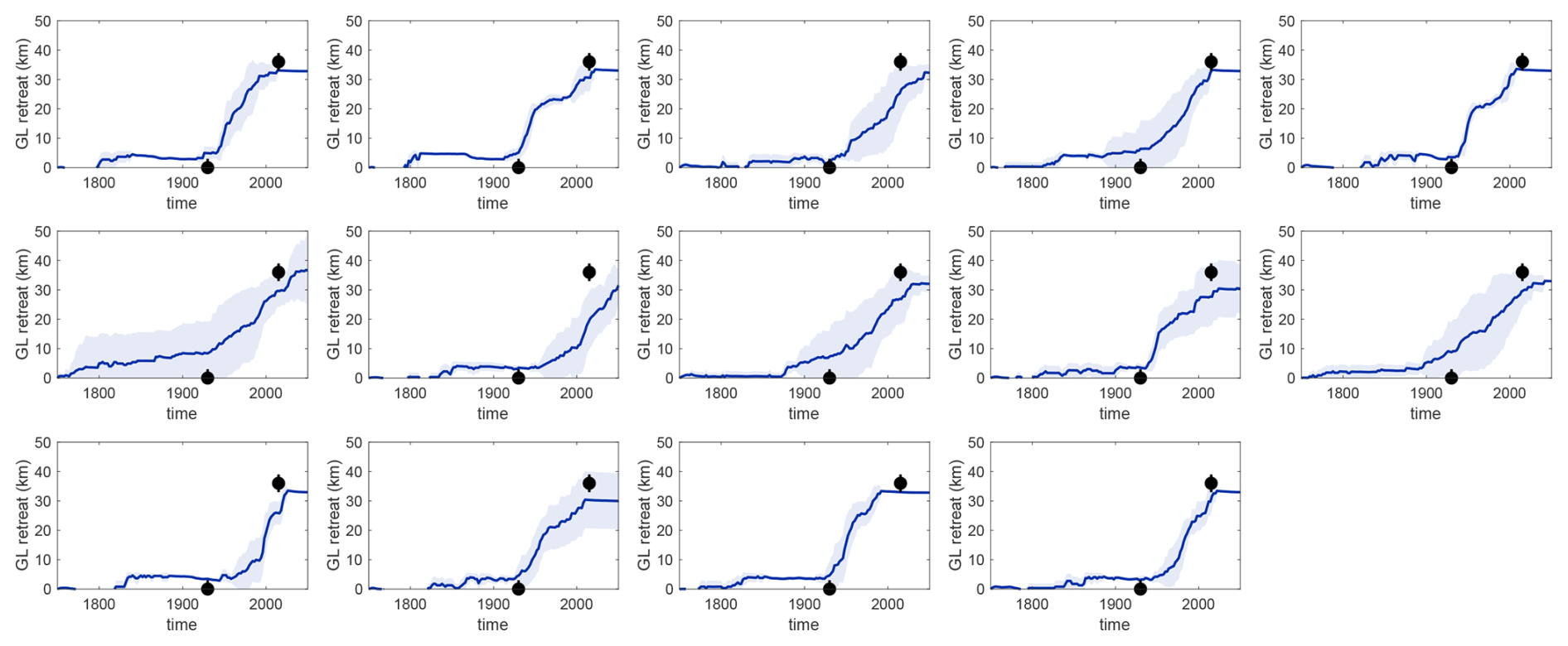
Figure 6 Trajectories of grounding-line retreat from posterior samples. Each panel corresponds to an individual realization of forcing. The shaded band indicates one standard deviation around the central estimate (solid curve). Black points with error bars indicate observational constraints.

In Fig. 7, we show trajectories of grounding-line retreat and grounded volume from all 140 samples from the posterior distributions. These trajectories (blue curves in Fig. 7) represent our best estimates of reconstructed grounding-line position and ice volume, accounting for both aleatoric and parametric uncertainty, given our choice of initial state. As for the trajectories for individual realizations of forcing, the posterior samples reproduce the observed retreat, albeit with a slight underestimation. Uncertainties in these trajectories are relatively small, indicating that, as for the posterior distributions, even our small number of observational constraints provides strong constraints on trajectories.

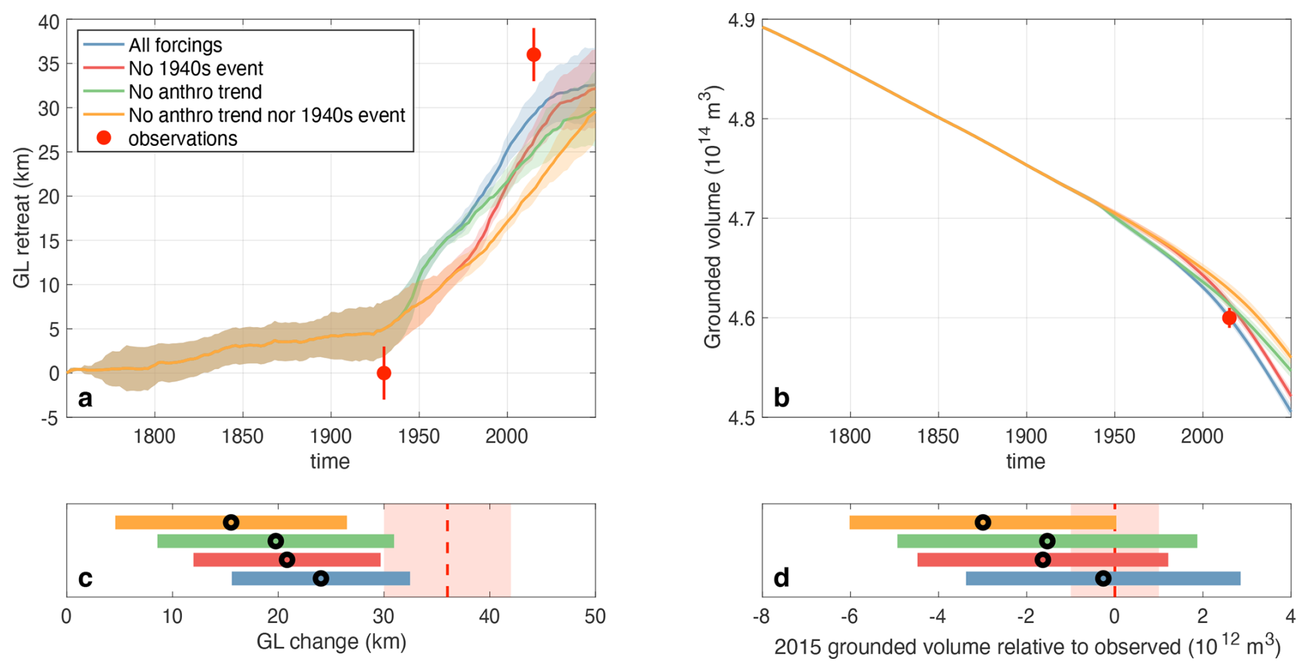
Figure 7 Trajectories of (a) grounding-line retreat and (b) grounded volume from posterior samples. Results are shown for several different ensembles as follows: all forcings (blue), with no 1940s event (red), no anthropogenic trend (green), and neither a 1940s event nor an anthropogenic trend (orange; see main text for an explanation of these scenarios). Shaded regions indicate one standard deviation around the central estimate (solid line). Note that the trajectories and shaded regions are indistinguishable for the four scenarios prior to the 1940s. Red points with error bars indicate observational constraints. Panels (c) and (d) indicate the mean (black circles) and standard deviation (solid lines) of distributions of grounding-line retreat between 1940 and 2015 and grounded volume relative to the 2015 value. Red dashed lines and shaded area indicate the central estimate and uncertainty in the observations, respectively.

In our statistical reconstruction, the grounding line remains pinned on the ridge until the 1940s, when retreat is initiated (Fig. 7a). This is consistent with the imposed observational constraint on grounding-line position in the 1940s. The grounded volume, however, decreases from the beginning of the simulation, with accelerating retreat beginning in the 1960s (Fig. 7b). The parameters selected by the procedure, which result from our experimental design (in particular, our three observational controls, combined with choice of initial state), effectively precondition the ice sheet to lose volume, but not experience grounding-line retreat, from the start of the simulation, with grounding-line retreat initiated in the 1940s. Without a pre satellite-era control on ice volume, it is difficult to ascertain whether, in reality, the ice sheet was losing mass over this entire period or not. An alternative scenario is that the ice volume was close to steady state for several hundred years prior to the satellite record, but that scenario cannot be considered by this analysis. Given that the grounding-line position is stable, but the ice volume decreases prior to the 1940s, the ice sheet is adjusting during this period to the change in parameter values imposed on it at the start of the simulation (the initialisation shocks discussed in Sect. 2). We do not know in advance how long these adjustment periods will be, because we do not know which parameters will be selected by the CES procedure. However for those parameters selected here, it appears to continue for some time into the simulation. Therefore, the effect of trends in forcing are likely obscured by these initial condition effects. In what follows, we therefore report all attribution results as conditional on our choice of initial state. We discuss possible solutions to this problem in the discussion.

In the previous section, we demonstrated that the observed retreat of PIG over the 20th century is consistent with a strong anthropogenic trend in forcing, and that it is likely there was a sustained anomaly in forcing in the 1940s. We now move on to assess how much additional grounding-line retreat and ice loss took place because of this likely trend and 1940s event. To do so, we construct three further ensembles of simulations, supplementing the posterior samples described above (referred to henceforth as the “all-forcings” ensemble). Each of these further ensembles are identical to the “all-forcings” ensemble, with 140 simulations, but with the following climate forcing components changed: in the first, all samples have no anthropogenic trend in forcing, i.e. T₀=0 (referred to as the “no-trend” ensemble); in the second, all samples have no 1940s event, imposed by setting B₀=0 (referred to as “no 1940s event” ensemble); in the third, all samples have no anthropogenic trend in forcing nor 1940s event ($T_{\mathrm{0}}=\mathrm{0},B_{\mathrm{0}}=\mathrm{0}$, referred to as “no trend nor 1940s event” ensemble).

Trajectories of grounding-line retreat and grounded volume for these ensembles are shown in Fig. 7. Prior to the 1930s, each of the four ensembles have identical trajectories. Shortly after the 1940s, trajectories in the “all-forcings” and “no-trend” ensembles display rapid grounding-line retreat, indicating that our reconstructions capture the role of the 1940s event as a trigger for the present phase of retreat. However, even in the “no 1940s event” and “no trend nor 1940s event” ensembles, grounding-line retreat still occurs after the 1940s (red and orange curves in Fig. 7), despite the anthropogenic trend in forcing only entering from 1960 (where present). We discuss this further in Sect. 4, but note that this is consistent with a picture of ice volume loss over the entire simulation period (Fig. 7b) discussed above: once the ice sheet has shrunk sufficiently, grounding-line retreat also initiated. By the 1970s, the effect of the anthropogenic trend starts to emerge: the all-forcings (blue) and no 1940s event (red) ensembles display enhanced grounding-line retreat rates compared to the no trend (green) and no trend nor 1940s event (orange) ensembles, respectively.

In Fig. 7c, we show distributions of grounding-line change between 1930 and 2015 in the four ensembles. Only in the all-forcings and no-trend ensembles is the ensemble mean plus one standard deviation within the observational range, accounting for the observational error (i.e. the right hand of the bars for the ensembles lies within the red shaded area). From this we see clearly how both the anthropogenic trend in forcing and 1940s event shift the distribution of grounding-line retreat towards enhanced retreat. However, consistent with the retreat of all ensembles, as outlined above, these shifts are not extreme and the distributions still overlap.

To quantify the role of the anthropogenic trend and 1940s event in the retreat of PIG, we compare the magnitude of retreat that has taken place in these ensembles by 2015. We focus on grounding-line retreat because, unlike the grounded volume, this metric is constrained prior to the satellite era. We calculate the fraction of attributable retreat as

$$\begin{array}{}\text{(16)}& \begin{array}{c}\text{fraction of}\\ \text{attributable retreat}\end{array}={\displaystyle \frac{\begin{array}{c}\mathrm{\text{all forcings retreat between 1930 and 2015}}-\\ \mathrm{\text{no trend retreat between 1930 and 2015}}\end{array}}{\mathrm{\text{all forcings retreat between 1930 and 2015}}}}\end{array}$$

The fraction of attributable retreat is interpreted as the fraction of the retreat which the anthropogenic trend in forcing is responsible for (a value of 1 would indicate that anthropogenic forcing is responsible for 100 % of the retreat). Our simulations indicate that the fraction of attributable retreat is 0.18. In other words, anthropogenic trends in forcing enhanced the retreat of PIG since the 1940s and are responsible for just under one fifth of the retreat over the industrial era, conditional on our choice of initial state. This is equivalent to an excess grounding-line retreat of 4.3 km.

Repeating the calculation (Eq. 16) for the 1940s event (i.e. replacing the no trend retreat with no 1940s event retreat in Eq. 16) reveals that 1940s event is responsible for around 13 % of the grounding-line retreat of PIG over the industrial era, corresponding to an excess grounding-line retreat of 3.2 km, conditional on our choice of initial state.

Figure 7a indicates that the anthropogenic signal in retreat has only just started to emerge (the green and blue lines have only recently deviated from one another). This begs the question of whether the anthropogenic signal of retreat will continue to persist beyond climatic noise. To address this question, we consider the evolution of the ensembles beyond the present day. To produce these future continuations, we extend the generation of autoregressive internal variability for each of the 14 realisations, and simply extend the pycnocline trends forward in time, where present, so that the pycnocline rises indefinitely (for upper end estimates of the trend in forcing, the pycnocline reaches the surface towards the end of the simulations, and no additional forcing occurs because all the water is at the temperature of the deep water).

In these simulations (Fig. 8a), the retreat of all ensembles temporarily stabilizes at a location roughly equivalent to the present day grounding-line position, by the mid-end of the 21st century. This position corresponds to a local topographic high (Fig. 1c), and is consistent with locations of relative PIG stability (Rosier et al., 2021; Reese et al., 2023). The all forcings and no 1940s event ensembles reach this position synchronously, at around 2050; by this time, approximately 100 years after it occurred, simulations have lost memory of the 1940s event. This highlights the long timescales on which even relatively short periods of anomalously high melting can influence glacial retreat. Between approximately 2075 and 2100, all four of the ensembles are grounded at or close to this local topographic high; during this time, the fraction of attributable retreat approaches zero (calculated by replacing the 2015 in Eq. 16 with the relevant year, Fig. 8b), i.e. the anthropogenic signal is undetectable in the grounding-line position.

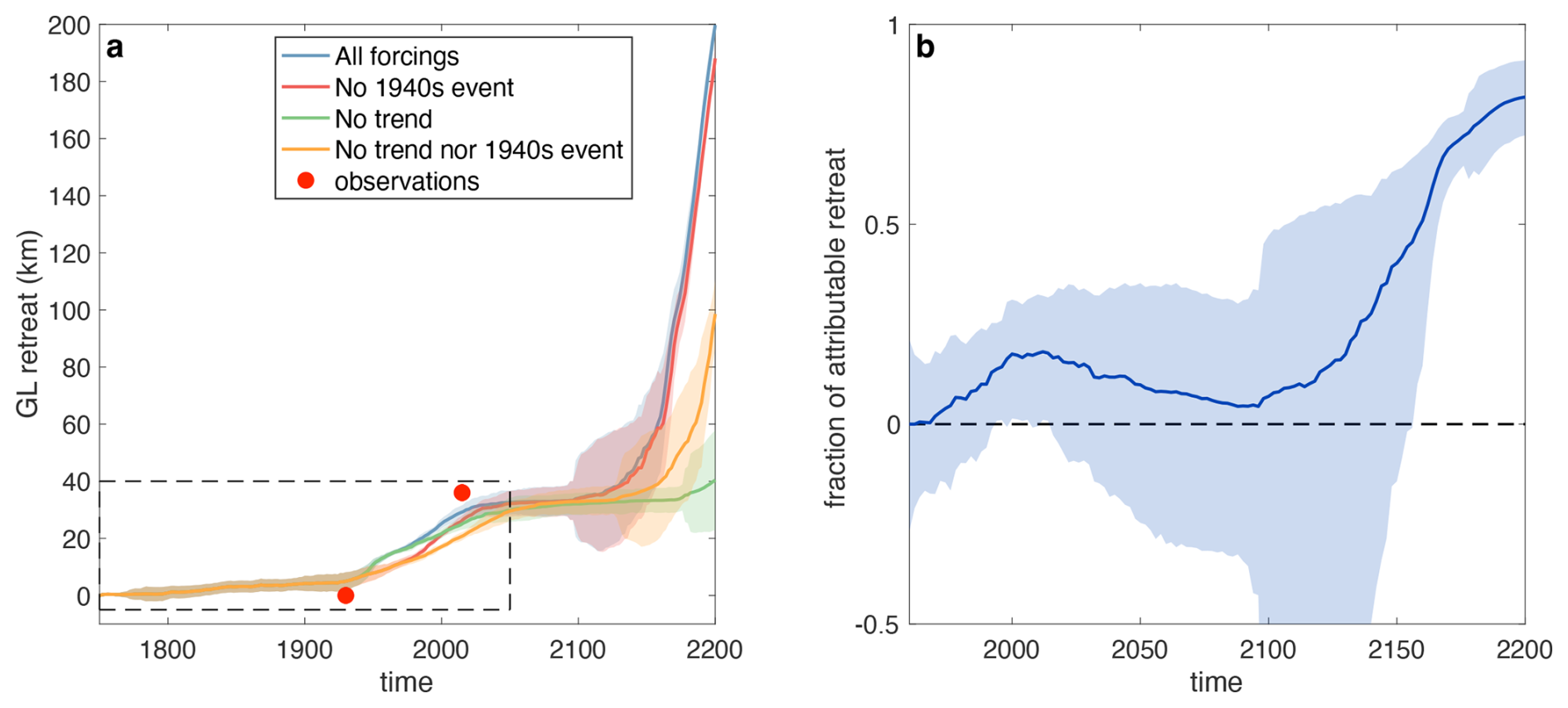
Figure 8 (a) As in Fig. 7a, but for simulations extended out until 2200. The dashed box indicates the area shown in Fig. 7a. (b) Time evolution of the fraction of attributable retreat (Eq. 16). The solid line shows the central estimate, obtained using the mean of trajectories shown in (a). The filled area shows the error in this quantity.

Around 2100, retreat is re-initiated in the central estimate of ensembles with an anthropogenic trend, while those without a trend remain at the topographic high for longer. Concomitantly, the fraction of attributable retreat increases (note that the ensemble spread increases beyond this because several ensemble members re-advance at this point). Essentially the fraction of attributable retreat is controlled by the persistence time at pinning-points, with anthropogenic trends in forcing leading to removal from these points sooner, as has been demonstrated to be a leading order control on future WAIS retreat rates (Bett et al., 2024). By 2150, the fraction of attributable retreat becomes significantly different from zero. Thus, our simulations suggest that while the anthropogenic signal in the retreat is detectable at present in PIG's grounding-line position, this will not persist beyond the 2030s, and the next time that this signal will be present is in the middle of the 22nd century. By 2200, almost all of the retreat is attributable to anthropogenic trends in forcing. We stress, however, that these projections are conditional on the idealised forcing scenario that the linear trend in anthropogenic forcing continues indefinitely.

We also note that deglaciation occurs sooner in the ensemble with no trend and no 1940s event, compared to that with just no trend. We suggest that is because of the role of history in the retreat (as we have elaborated above): the retreat in the no trend no event ensemble over the 1950–2050 period occurs more steadily, which we suggest preconditions it for sooner retreat off the temporarily stable ridge.

4 Discussion

In this paper, we have made progress in two areas: firstly, we have demonstrated how the calibrate-emulate-sample framework (Cleary et al., 2021) may be used to efficiently infer observationally-constrained posterior distributions of model and climate forcing parameters in ice sheet models; and, secondly, we have used the results of this to perform an attribution assessment on the retreat of the PIG over the industrial era and into the future. These simulations suggest that it is unlikely that the magnitude of industrial era PIG retreat would have occurred without an anthropogenic trend in forcing and that the likely trends in forcing that occurred since the 1960s enhanced the retreat of PIG. We have quantified this effect, finding that anthropogenic trends in forcing since the 1960s are responsible for approximately 18 % of the PIG retreat over the industrial era. Our analysis also indicates that the 1940s event, which was synchronous with the beginning of the phase of rapid retreat (Smith et al., 2017), played an important role in the retreat of PIG over the industrial era. These results are conditional on our choice of initial state, which, after having completed the CES procedure, imposes that PIG must lose mass consistently since 1750 to reproduce the observed ice volume in 2015. The overall response is a combination of a contribution from the initialization shock and a contribution from 20th century forcing components (the 1940s event and the anthropogenic trends), but we cannot disentangle these with our setup. If we removed the effects of initialisation shock (for example, by allowing the procedure to also pick the initial state, as outlined above), then the response would be purely a result of the 20th century forcing or long-term thinning trends. We therefore conclude that the precise quantified role of 20th century forcing components is highly uncertain.

Our study is, to the best of our knowledge, the first to quantify the role of anthropogenic trends in forcing on retreat of an individual glacier in an ice sheet (i.e. not a mountain glacier). This study builds upon frameworks for attributing retreat of such glaciers (Christian et al., 2022; Bradley et al., 2024b) and supports the growing literature on attribution of mountain glacier retreat (Vargo et al., 2020; Stuart-Smith et al., 2021; Marzeion et al., 2014; Roe et al., 2021) demonstrating that anthropogenic forcing has a strong influence on glacier evolution.

As discussed, our results are conditional on the choice of initial state and experimental setup. It may be that this initial state is accurate, in which case our results suggest that PIG has been losing volume consistently over the industrial era. This would suggest that the ice sheet state prior to the industrial era was not stable, supporting the hypothesis that the long, slow retreat of the WAIS since the last glacial maximum is an important contributor to the current phase of retreat, with anthropogenic trends in forcing since the 1960s expediting retreat. In our experiments, we included (parametrisations of) what we thought were the two main contributors to forcing: the 1940s event and the anthropogenic trend. However, the results of the experiments suggests that we require a refocus on the quantification of the preindustrial volume and conditions, in addition to the 1940s bump and trend, and that pre-industrial ice sheet trends in forcing may also have an important role to play and should be considered in future attribution studies of the West Antarctic Ice Sheet.

The alternative hypothesis to the correct initial state is that the imposed initial state is larger than it should be in practice. In this case, the interpretation of our results is that the CES procedure selects the parameters which are consistent with retreat being initiated in the 1940s, regardless of the 1940s event or anthropogenic trends in forcing after the 1960s. This picture is confused by initialization shocks, which, in our framework, are necessary step changes in the forcing and model parameters at the start of the simulations; the model's response to these changes appears to blur into the effects of 20th century climate forcings of interest. Without pre-satellite era controls on ice volume, distinguishing between these two hypothesis is difficult.

To address these potentially important initialization issues, we recommend that the initial state and historical forcing be treated as additional parameters to be constrained by the CES procedure. The former could be achieved, for example, by scaling the size of the ice volume by a prefactor (we effectively took a prior distribution on this parameter to be a delta function, with no uncertainty), or perhaps by including an extra parameter that defines a shift to the initialization date. More generally, our results highlight the importance of selecting an appropriate initial state when simulating retreat of the Antarctic Ice Sheet.

For the particular system considered here, using the CES procedure, only a small number of observational constraints can provide strong controls on permissible model parameters, resulting in narrow (relative to the priors) posterior distributions of model and climate parameters. It is important to stress that the CES procedure is generic (Cleary et al., 2021): all that is required is to construct an array of model–observation errors for the system that is being modelled. Ice sheet and glacier systems are typically highly non-linear and thus the space of likely parameters may be small. In these cases CES may be particularly effective at constructing observationally constrained posterior distributions and therefore be an effective parameter calibration method for ice sheet and glacier models. For the system considered here, the EKI embedded within CES outperforms latin hypercube sampling, the current state of the art in ice sheet modelling.

The procedure applied here can also be considered a transient calibration of ice sheet model parameters over a long period (though using fewer observations and with fewer parameters in the control space – several scalars rather than whole fields – than other transient calibration studies (e.g. Goldberg et al., 2015)). Our calibrated simulations suggest that PIG will soon stabilise at a local topographic high, close to its present day grounding-line position. It will remain grounded at this local topographic high for approximately 100 years, before accelerating rapidly in the middle of the 22nd century. These results assume that anthropogenic trends in forcing persist indefinitely. Ocean simulations suggest, however, that ocean forcing could accelerate in the coming decades (Naughten et al., 2023), regardless of the emissions pathway followed, potentially expediting this retreat. In addition, these projections implicitly assimilate (through both the initial sampling of parameters in the EKI and in the update step of the MCMC) prior distributions of model and climate forcing parameters. In this case, the prior distributions nudge the model towards lower retreat than suggested by observational constraints. Thus, future retreat may be faster than our simulations suggest.

We also made several choices during the CES procedure, which should be noted. Firstly, we chose to use observations of grounding-line position in 1930 and 2015, and grounded volume in 2015. There are a wide variety of satellite observational datasets available which we which could have further assimilated into the procedure. However, we elected not to as most of these are already used in the inversion, so are already taken into account in the full methodology. In addition, for the CES procedure to work well in this instance, all we need are large scale bulk metrics that are well spread over time, to constrain the centennial evolution. Satellite observations are good to constrain the present-day inversion, but weaker for the CES machinery as their changes over the modern observational era are small on the scale of the 1940s–present changes. In addition, including further present day observations into the procedure naturally down-weights the 1940s observations which are crucial and only create one data point (we have already prioritised the present day somewhat by including both volume and grounding-line position for 2015). Secondly, we use Gaussian processes to emulate these observations and, in particular, individual Gaussian processes for each of the observational constraints. We chose to emulate the observational constraints individually as, when attempting to emulate them all simultaneously, we encountered convergence issues arising from the fact that the matrix required to be inverted during the training process is poorly scaled. Our choice of Gaussian processes enables us to obtain uncertainty estimates in emulated values of these quantities, which are propagated through to attribution assessments via posterior distributions of model parameters. Given that our emulator displays good performance, and our results include emulator uncertainties, we do not believe that the results would change if another, different emulator with similar performance was chosen, but future work should investigate the sensitivity of posterior distributions to the choice of emulator.

In addition, we have used present day, time-invariant ice viscosity in our simulations; in the past, however, the Pine Island Ice Shelf likely had higher structural integrity (Lhermitte et al., 2020) and thus lower effective viscosity; as the ice shelf continues to degrade in the future, its buttressing effect will reduce, expediting retreat. Additionally, loss of ice shelf area, not included in our model, may encourage ice sheet retreat either directly via loss of buttressing (Joughin et al., 2021) or indirectly via changes in basal melt rates (Bradley et al., 2023, 2022; Yoon et al., 2022).

Projected future increases in accumulation may, however, offset future ice losses (we assume constant accumulation in this study). This assumption may also obscure attribution assessments: although reconstructed WAIS surface mass balance shows no trend since 1800, there is a negative trend over the past 1000 years (Thomas et al., 2017). These longer timescale trends might have enhanced ice sheet retreat, underscoring the role of longer term trends in the present phase of WAIS retreat. Here, we focussed on trends in ocean forcing because it is understood to be the dominant driver of recent WAIS retreat (Shepherd et al., 2004; Pritchard et al., 2012), but future attribution assessments should also consider trends in accumulation.

Our study demonstrates that it is possible to attribute the component of retreat of glaciers in the Antarctic Ice Sheet due to anthropogenic climate change. As the World's ice sheets continue to represent an ever-increasing fraction of the global sea level rise budget (IPCC, 2022), such studies will pave the way for global attribution assessments of sea level rise, building upon those from other sources of sea level rise particularly mountain glaciers (Roe et al., 2021; Marzeion et al., 2014) and thermosteric sea level rise (Slangen et al., 2014). Attribution studies are increasingly used to support recourse for the harms associated with anthropogenic climate change both in the courtroom (Marjanac and Patton, 2018) and in policy (Burger et al., 2020); therefore, studies attributing retreat of glaciers to anthropogenic climate change may play an important role in supporting recourse for the harms associated with sea level rise.

5 Conclusions

In this paper, we have used the calibrate-emulate-sample procedure to quantify the role of anthropogenic trends in forcing on the retreat of the Pine Island Glacier over the industrial era. We have demonstrated that the CES procedure is effective at constraining model and climate forcing parameters, even when only a small number of observational constraints are assimilated. We find that it is unlikely that the extent of the observed PIG retreat over the industrial era would have occurred without anthropogenic trends in forcing. In addition, anthropogenic trends in forcing almost certainly increased the industrial era retreat of PIG. These trends are responsible for an extra 18 % of the retreat over this period. These results are conditional on our choice of initial state, which, after having completed the CES procedure, imposes that PIG must lose mass consistently since 1750 to reproduce the observed ice volume in 2015. The overall response is a combination of a contribution from the initialization shock and a contribution from 20th century forcing components (the 1940s event and the anthropogenic trends), but we cannot disentangle these with our setup. We therefore conclude that the precise quantified role of 20th century forcing components is highly uncertain.