A multisensor C-band synthetic aperture radar (SAR) approach to retrieve freeze/thaw cycles: a case study for a low Arctic environment

This study investigates the spatial variability of surface freeze/thaw (F/T) cycles in low arctic tundra retrieved from multisensor SAR backscatter time series. To increase the temporal resolution of SAR observations, we combined measurements from Sentinel-1 and RADARSAT-2. An incidence angle normalization was applied to the backscatter time series to remove the influence of the acquisition angle on backscatter. A seasonal threshold algorithm (STA) was used to detect F/T transitions and applied to HH, HV and HH+HV polarization datasets. The classification threshold was optimized using soil temperature measurements from spatially distributed sites. A detection accuracy of over 93 % was calculated with an optimized classification threshold of 0.62 for the HH+HV time series on those sites. We created surface F/T day of the year (DOY) maps of the study area for the 2018 and 2019 freezing transitions, and for the 2019 thawing transition using the HH+HV time series with the optimized classification threshold. Those maps were combined with a terrestrial ecosystem (ecotype) map to investigate the impact of ecotypes on the F/T transitions. Three generalized least squares (GLS) models were fitted on the coupling of the maps. Differences of about 2–3 d were observed between ecotype classes. Based on these differences, we hypothesize that differences during the freezing transition were probably due to the underlying soil moisture and during the thawing transition, to the influence of vegetation. Our study demonstrates the power of merging two C-band SAR time series to create near-daily F/T maps over arctic environment to allow for better understanding of surface F/T processes happening at small spatial scale in arctic environments.

1 Introduction

Over the last 4 decades, important signs of climate change have been observed across the Arctic (Dai et al., 2019) amplified by enhanced warming due to positive climate feedback (Serreze and Barry, 2011). The observed increase in surface temperatures at two to three times the rate observed elsewhere on the planet has significant impacts on the cryosphere and arctic ecosystems. Increased air temperature across the Arctic influences several cryosphere-related phenomena, such as the precipitation type and phase (Jeong and Sushama, 2018; Langlois et al., 2017), the snow cover accumulation and distribution (Derksen and Brown, 2012), the spatial and temporal evolution of vegetation cover (Bjorkman et al., 2018; Martin et al., 2017), and the soil thermal regime (Smith et al., 2010), including permafrost temperature and active layer depth.

The permafrost active layer refers to the soil surface layer which undergoes an annual freeze and thaw (F/T) cycle. This cycle impacts the surface energy budget (Schuur et al., 2015), hydrological and carbon cycles (Wang et al., 2009), vegetation growing seasons (Kim et al., 2012), underlying permafrost state and active layer thickness (ALT; Yi et al., 2019). Snow strongly influences those processes because of its low thermal conductivity and its high albedo that regulate ground temperatures (Domine et al., 2018b; Zhang et al., 2018). As such, snowpack properties like total depth, density, and microstructure influence the F/T cycles of the underlying soil (Prince et al., 2019). However, one of the most significant consequences of a warming Arctic is a reduction in snow cover duration with the snow cover forming later in the fall and melting early in the spring (Derksen and Brown, 2012; Brown et al., 2017). Furthermore, tundra vegetation, which modulates snow distribution through trapping effects (Barrere et al., 2018; Busseau et al., 2017; Royer et al., 2021), is also changing significantly (Bjorkman et al., 2018; Martin et al., 2017). Royer et al. (2021) suggested that changes in the snowpack microstructure and distribution patterns, linked to the increase of vegetation height and coverage, could further amplify permafrost warming (Callaghan et al., 2011). These complex soil/vegetation/snow interactions closely tied to FT cycles govern a large part of carbon fluxes in Arctic environments. On one hand, FT processes control the growing season length in arctic environments, where the period of productivity and carbon sequestration through photosynthesis for plants is short and critical for the ecosystems. Hence, changes of few days in FT processes could lead to significant change in the growing season length of certain species potentially leading to important ecological impacts (Gehrmann et al., 2022). On the other hand, soil FT also govern the soil carbon emission through temperature and the availability of liquid water for microbial activity in the soil (Natali et al., 2019; Mavrovic et al., 2023, 2025). Hence, during the zero curtain, which can last from several days to few weeks depending on the soil moisture regime in tundra environments (Davesne et al., 2022), the soil temperature's near-freezing state can sustain microbial activity, which has significant implications for carbon fluxes where can have similar total or probably higher emissions to the rest of the winter (Arndt et al., 2022). Knowing the critical importance of spatio-temporal variation of FT cycles on Arctic ecosystems, it is though essential to improve our capacity to monitor FT processes and high temporal and spatial resolution over Arctic environments.

Several studies have developed F/T detection algorithms using satellite passive microwave (PMW) measurements (Chen et al., 2019a; Derksen et al., 2017; Kim et al., 2011; Prince et al., 2018; Rautiainen et al., 2016; Roy et al., 2015, 2020; Xu et al., 2016; Zheng et al., 2017). The potential of using low-frequency passive microwave data for developing F/T cycle detection algorithms have increased due to the available L-Band satellite missions (e.g., Aquarius, SMOS, SMAP). Despite the clear potential for detecting and monitoring soil F/T cycles, the strong landscape heterogeneity within the coarse grid spacing of these datasets (∼25 km) leads to a misrepresentation of the spatial variability, biases, and uncertainty in the F/T retrievals (Ponomarenko et al., 2019; Prince et al., 2019).

Satellite Synthetic Aperture Radar (SAR) measurements fill this gap, because of their much finer spatial resolution: typically, from 1 to 100 m. The SAR backscatter signal (sigma nought; σ⁰) depends on the dielectric (e.g., moisture and water phase) and geometric (e.g., roughness) properties of the target, leading to a strong sensitivity to dielectric contrasts during soil surface phase transition seasons (i.e., freezing and thawing). Given the very high dielectric constant of water in the microwave spectrum, the dielectric constant for dry or frozen soil is small compared to that of wet or thawed soils (Ulaby et al., 1986). SAR backscatter information can thus help to detect changes in the dielectric constant of the soil surface during F/T cycles for different ecosystems such as agriculture (Baghdadi et al., 2018; Fayad et al., 2020; Taghipourjavi et al., 2024), forested (Jagdhuber et al., 2014; Cohen et al., 2021; Cohen et al., 2024; Moradi et al., 2024) and permafrost covered (Park et al., 2011; Chen et al., 2019b, 2022; Zhou et al., 2022; Taghavi-Bayat et al., 2024; Bartsch et al., 2025) environments. C-Band SAR observations generally allow to get the signal from the soil top layer with a limited penetration depth of about 5 cm depending on the properties of the soil (Ulaby et al., 1986). The easy access to PMW data and its daily temporal coverage have favoured their use compared to SAR data in the detection of F/T cycles (Park et al., 2011). However, constellations such as Sentinel-1 (since 2016; Bourbigot et al., 2016) and the RADARSAT Constellation Mission (RCM; since 2019) allow improved temporal coverage of σ⁰ data, thus increasing the potential for daily observations across the Arctic.

This study aims to retrieve surface F/T cycle onset in a low arctic tundra environment using SAR backscatter time series. This paper thus aims to (1) create a near-daily multisensor C-band normalized backscatter time series, and (2) evaluate those time series' potential to retrieve surface F/T cycles, using a simple seasonal classification algorithm and a study site in a low arctic environment. This case study relies on a unique ecotype map created from unsupervised classification of 2011 WorldView-2 multispectral imagery (Ponomarenko et al., 2019) based on the Canadian arctic-subarctic Biogeoclimatic Ecosystem Classification (CASBEC) defined in McLennan et al. (2018).

2 Study site and data

2.1 Overview of the study area

This study focuses on the Intensive Monitoring Area (IMA) north of the Greiner Lake watershed, near Cambridge Bay, Victoria Island, NU, Canada (Fig. 1). The site is instrumented with a meteorological station and characterized by low and sparse vegetation, low annual precipitation, and flat topography, typical of arctic tundra environments. The IMA region was chosen due to the availability of a unique high-resolution detailed ecotype map (Sect. 2.2.3) which will be used for the small-scale spatial variability case study. The mean annual air temperature is around −10 °C, and rarely goes above 18 °C during the warm season or below −41 °C during the cold season. For our study, we used daily soil temperature data derived from a spatially distributed network of i-Buttons deployed across the IMA over 2018–2019, in the most dominant ecotypes (Ponomarenko et al., 2019) present in the area (Fig. 1).

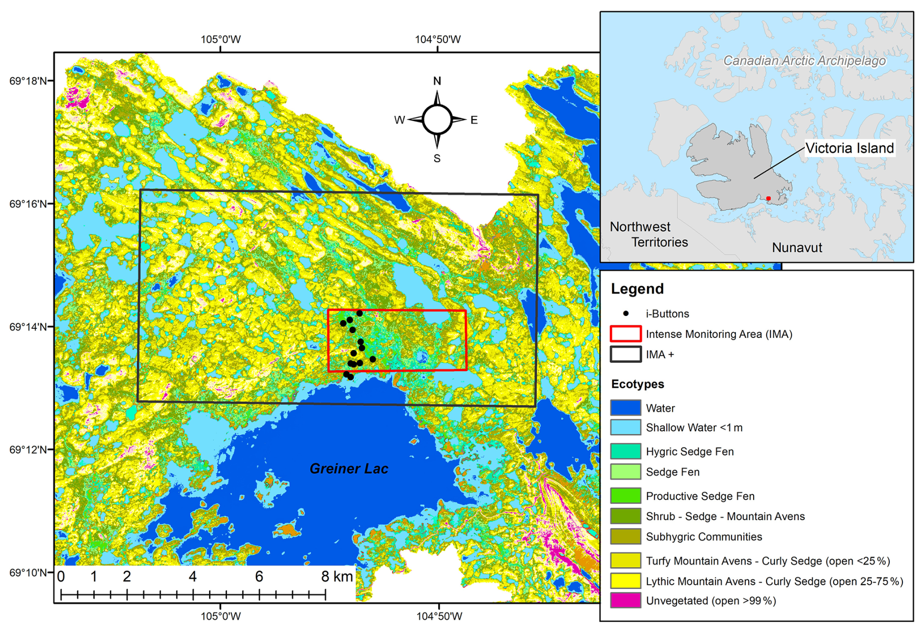
Figure 1 Study site of the IMA (red) and the extent covered by the F/T maps created in this study referred to as the IMA+ (black) near Cambridge Bay, Victoria Island, NU, with the ecotypes as a base map and i-Button locations. Legend of the ecotypes only includes dominant classes.

2.2 Data Description

2.2.1 Soil and air temperature

We developed and validated the F/T detection algorithm based on reference soil (T_soil) and air (T_air) temperature data (Fig. 2).

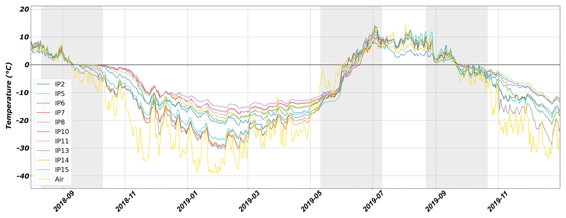
Figure 2 T_soil for the 10 reference sites (IP) and T_air from ECCC for the study period of August 2018 to December 2019 with the transition seasons (in grey) for freezing in 2018 and 2019 and thawing in 2019.

Soil temperature

Soil temperature (T_soil) was measured using low-cost sensors (i-Buttons) deployed within the IMA over 2 years from July 2018 to mid-July 2019 in ten sites; and from mid-July 2019 to August 2020 in seven of the ten previous sites. The i-Buttons measured the soil temperature every three hours and have been placed at three depth ranges in the soil: from 2 to 4 cm; from 10 to 20 cm and from 20 to 30 cm in the following sites (IPX): Hydric sedge fen (IP2), Sedge fen (IP7, IP8 and IP14), Productive sedge fen (IP6 and IP11), Subhygric communities (IP5 and IP10), Turfy mountain avens – Curly sedge (open <25 %) (IP15), and Unvegetated (open >90 %) (IP13) as detailed in McLennan et al. (2018). Only the i-Buttons located at the surface (first 4 cm of the soil) were used in the study, since C-band measurements are sensitive to changes near the surface and show limited soil penetration (Rowlandson et al., 2018). A fixed uncertainty of 0.5 °C was considered on the data since the observed biases are within the manufacturer's precision (Prince et al., 2019). Soil temperatures were averaged daily since daily soil temperature variability is of the order of the i-Buttons uncertainty. The surface was considered frozen when T_soil≤0.5 °C and thawed when T_soil>0.5 °C according to i-Button data, considering its accuracy and the clear zero curtain observed around 0 °C during the freezing in fall (Fig. 2). The zero curtain refers to the extended period during the freezing or thawing of the soil where the temperature stays around 0 °C due to the release of the residual latent heat or water in the soil (Domine et al., 2018a). Surface freezing (D_fr) and thawing (D_th) reference transition day of the year (DOY) were derived from the daily mean T_soil. D_fr(soil) was defined as the first day of a series of 7 consecutive days when the surface was considered frozen for every i-Buttons, and D_th(soil), as the first day of a series of 7 consecutive days considered thawed.

Air temperature

Average daily air temperature (T_air) data for 2018 to 2019 were obtained from the Environment and Climate Change Canada meteorological station (ECCC, https://climat.meteo.gc.ca/historical_data/search_historic_data_f.html, last access: April 2026) located at the Cambridge Bay airport, about 15 km from the IMA. Global reference transition DOY (D_th(air) and D_fr(air)) were calculated from T_air as the first day of a series of 7 consecutive days classified as frozen (T_air≤0 °C) or thawed (T_air>0 °C). Since T_air is considered constant over the study site, reference transition seasons were derived as ±30 d around D_th(air) and D_fr(air) (grey area in Fig. 2).

2.2.2 Synthetic Aperture Radar (SAR) dataset

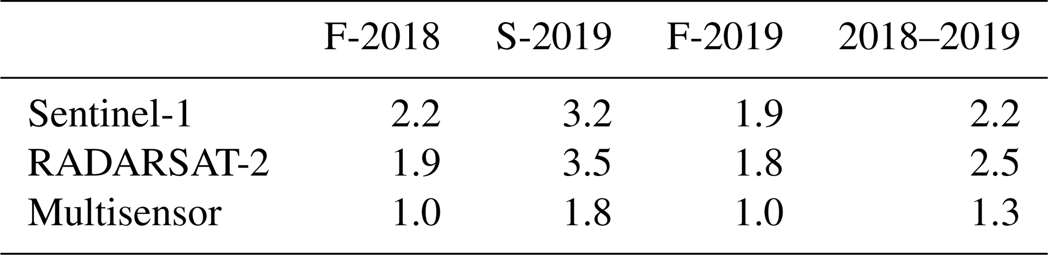
In this study, we used the C-band SAR backscatter obtained from the sensors of two satellite missions, namely the Sentinel-1A-1B constellation (available since 2016), and RADARSAT-2 (made available for this study between August 2018 and December 2019). Both SAR operates at a center frequency of 5.405 GHz. This study focuses on the period spanning from August 2018 to December 2019, where the overlap between both data source allows for quasi-daily revisit time in the transition seasons of Fall 2018 (F-2018), Spring 2019 (S-2019) and Fall 2019 (F-2019). Using both sensors, the average revisit times are respectively 1 d for F-2018 and F-2019, and approximately 2 d for S-2019 (see Table 2 in Sect. 3.1). Both datasets were preprocessed independently with a standardized processing chain (Sect. 3.1) and resampled to a standard 50 m × 50 m grid to be combined into one multisensor time series. Note that all Sentinel-1A-1B and most RADARSAT-2 observations were taken around 13:00 UTC. Hence, only 14 % of SAR observations were taken around 00:00 UTC (all RADARSAT-2 observations).

Sentinel-1A-1B

We used 270 Level-1 GRD Extra Wide Swath (EW) images from Sentinel-1A-1B in dual polarization (HH, HV) with a grid spacing of 40 m × 40 m. Due to the combination of measurements from multiple orbits, the acquisition incidence angles ranged from 20 to 46°. Descending/ascending scenes were used together.

RADARSAT-2

We used 200 ScanSAR wide SAR Georeferenced Fine product (SGF) RADARSAT-2 images in dual polarization (HH, HV) with a 50 m × 50 m grid spacing. We also used multiple orbits with an acquisition incidence angle ranging from 20 to 49°, including both descending and ascending scenes.

2.2.3 Ecotypes map

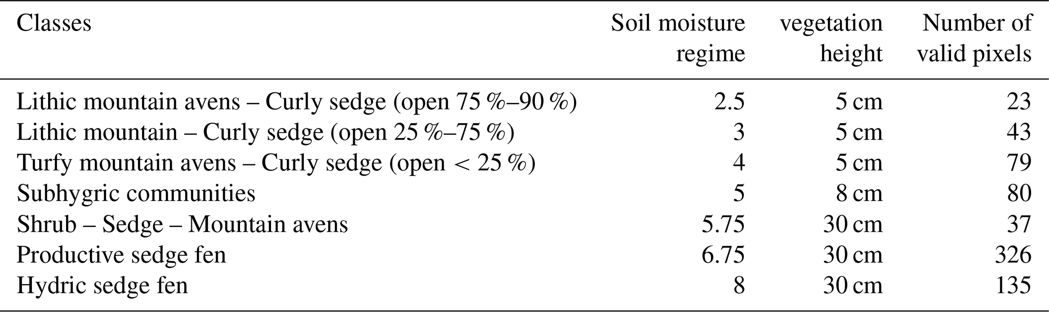
This study also presents a case study relying on a unique ecotype map created from unsupervised classification of 2011 WorldView-2 multispectral imagery (Ponomarenko et al., 2019) based on the Canadian arctic-subarctic Biogeoclimatic Ecosystem Classification (CASBEC) defined in McLennan et al. (2018). The CASBEC classification is based on terrestrial ecosystems (i.e., ecotypes) and includes vegetation characteristics, as well as the soil moisture regime (SMR). The ecotypes are mapped for Greiner Lake's watershed at a spatial resolution of 10 m and contain 19 map units regrouping 21 ecotypes. Resampling the 10 m × 10 m map to a 50 m × 50 m grid allowed to match the SAR imagery time series resolution. The analysis only included the pixels where 90 % of the original 10 m × 10 m pixels within a 50 m × 50 m pixel have the same ecotype value. Waterbodies and ecotype classes with pixel count smaller than 20 were also excluded from the case study analysis. Table 1 present the number of pixels left from the resampling for the remaining ecotype classes. More details on the ecotypes can be found in Ponomarenko et al. (2019) from which a summary of the key characteristics relevant to this study are presented in Table 1: the soil moisture regime (SMR) and the vegetation height. The soil moisture regime is defined by a scale ranging from 0 to 9, where 0 is very xeric and 9 is aquatic.

Table 1 Ecotypes classes found in the IMA+ and used inside the spatial analysis of F/T onset with soil moisture regime (SMR) and vegetation height (Ponomarenko et al., 2019).

3 Methods

3.1 SAR processing

Both SAR datasets were preprocessed independently using a common chain (Fig. 3), which includes radiometric calibration, speckle filtering, orthorectification and incidence angle normalization. PCI Geomatica functionality with python scripts were used in the study. First, we applied a radiometric calibration to the backscatter coefficient (σ⁰). The calibration removed the dependency of the observation to the sensor characteristics; allowing us to combine the datasets from both sensors. To decrease spatial noise in each image, we then applied a Lee speckle filter with a window of 7 pixels×7 pixels. Finally, to allow the combination of dataset, images were then orthorectified to a fixed grid of 50 m×50 m using a cubic interpolation method. The orthorectification was performed with the rational function model and the ArcticDEM digital elevation model at 2 m (Porter et al., 2023).

Figure 3 Flowchart of the SAR imagery (i.e., Sentinel-1 and RADARSAT-2) preprocessing.

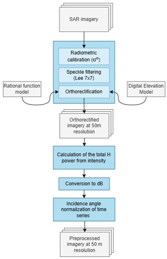
Since this study focuses on dual polarization (i.e., horizontally transmitted, horizontally or vertically received), the total measured power in horizontal polarization (referred to as Total H power or HH+HV) then corresponds to the sum of both intensities (Woodhouse, 2006). The Total H power was calculated as one new time series and was used in the ecotype analysis (Sect. 3.4). The three time series (i.e., HH, HV and HH+HV) were then converted to decibels (dB).

Radar backscatter values were normalized for the different incidence angles of the various orbits used in this study. A linear regression between the backscatter coefficient (σ⁰; in dB) and the incidence angle (θ_incidence; in degrees) was calculated for each pixel independently such as

$$\begin{array}{}\text{(1)}& {\mathit{\sigma }}^{\mathrm{0}}\left({\mathit{\theta }}_{\text{incidence}}\right)=\mathit{\alpha }\cdot {\mathit{\theta }}_{\text{incidence}}+\mathit{\beta }\end{array}$$

where α represents the slope of the relation and β, the intercept (Chen et al., 2019; Mäkynen et al., 2002; Widhalm et al., 2018). During the thawed season, important changes in biomass and soil moisture levels influence the signal evolution. Therefore, the relationship between the incidence angle and the backscatter is less significant than in winter, where those changes are less likely to impact the backscatter between acquisitions (Chen et al., 2019). The α calculated from the regression using the backscatter during frozen period was then used to explain the year-round angular dependency for the datasets. The slope (α) was then calculated for each pixel independently for periods when the surface is considered completely frozen (DOY 1–60 for Sentinel-1, and DOY 305–365 and 1–60 for RADARSAT-2) for the combination of 2018, 2019 and 2020 when available. The temporal periods for both sensors were chosen to get similar sample sizes for the same period. The time series were normalized at the median incidence angle of 34° as:

$$\begin{array}{}\text{(2)}& {\mathit{\sigma }}_{\mathrm{34}}^{\mathrm{0}}={\mathit{\sigma }}^{\mathrm{0}}-\mathit{\alpha }\cdot ({\mathit{\theta }}_{\text{incidence}}-{\mathrm{34}}^{\circ })\end{array}$$

Sentinel-1 and RADARSAT-2 time series were then combined to create a multisensor time series with a quasi-daily mean temporal resolution for all three transition seasons (Table 2).

Table 2 Mean temporal resolution (in days) of the combined Sentinel-1/RADARSAT-2 normalized datasets for three transition seasons and for the whole time series (2018–2019).

3.2 F/T detection algorithm

This study applies an empirical detection algorithm to identify the surface F/T state, using the same approach as the SMAP L3 EASE-Grid Freeze/Thaw State product (Derksen et al., 2017). The algorithm uses seasonal reference values to calculate a scale factor that is then classified into frozen or thawed state using a defined threshold (Rautiainen et al., 2016, 2014). Based on the work of Roy et al. (2015), using passive microwave data, we compared three methods to calculate seasonal reference values (Sect. 4.2.1). The first method (“average”) uses the average backscatter coefficients for a period during which, based on soil and air temperature measurements, the soil is completely frozen (1 December 2018 to 1 April 2019; σ_fr) or completely thawed (1 July 2019 to 1 September 2019; σ_th). The second method (“median”) uses the median backscatter coefficients over the same periods. Finally, the third method (“average-5”) uses the average of the five lowest backscatter observations during the frozen period, and the average of the five highest backscatter values during the thawed period. Frozen (σ_fr) and thawed (σ_th) seasonal reference values are calculated for every pixel independently, and subsequently used to calculate the seasonal scale factor (Δ) for every observation at time t as:

$$\begin{array}{}\text{(3)}& \mathrm{\Delta }\left(t\right)={\displaystyle \frac{\mathit{\sigma }\left(t\right)-{\mathit{\sigma }}_{\text{fr}}}{{\mathit{\sigma }}_{\text{th}}-{\mathit{\sigma }}_{\text{fr}}}}\end{array}$$

where σ(t) is the backscattering coefficient for one pixel at time t. Each standardized Δ(t) values are then classified as frozen or thawed with a defined threshold (T) such that:

$$\begin{array}{}\text{(4)}& \left\{\begin{array}{l}\mathrm{\Delta }\left(t\right)\le T\to \text{Frozen}\\ \mathrm{\Delta }\left(t\right)>T\to \text{Thawed}\end{array}\right.\end{array}$$

The threshold (T) was optimized by calculating the accuracy of the classification for threshold values ranging between 0 and 1, at an increment of 0.01 using Eq. (5) on the ten reference sites. D_th-fr(sol) and D_th-fr(air) were used as reference values to calculate the amount of good observation (#good observation) for the classification with every increment of thresholds (Sect. 4.2.2).

$$\begin{array}{}\text{(5)}& \text{Accuracy}\left(\mathit{\%}\right)={\displaystyle \frac{\mathit{\#}\text{good observation}}{\mathit{\#}\text{total of observations}}}\cdot \mathrm{100}\end{array}$$

3.3 Case study

3.3.1 Surface F/T maps

The optimized threshold, defined with the ten reference sites, was then used to create the surface F/T maps covering the IMA and its surroundings (IMA+; Fig. 1). The algorithm was applied on a cell-by-cell basis to retrieve the transition onset for F-2018, F-2019 and S-2019. We applied a hydrographic mask to remove any non-terrestrial pixel. Pixels with equal or higher frozen than thawed reference values (σ_fr≥σ_th) were also discarded. The temporal evolution of the backscatter in those cases did not allow for the detection of the dielectric discontinuity between soil state during the transition seasons, potentially linked to the presence of rocks of higher rugosity inside the pixels. Also, since T_air was considered constant across our study area, detected freezing and thawing dates falling outside the 60 d periods defined around D_th(air) and D_fr(air) were considered false detections, and were therefore discarded during the creation of the surface F/T maps. We chose to use the Total H power for the creation of the F/T maps to decrease the impact of the target orientation (e.g., vegetation distribution). Furthermore, by using this approach, we also increased the signal-to-noise ratio (SNR; Entekhabi et al., 2014), linked to the increase in signal quantity.

3.3.2 Ecotypes analysis

To analyze the impact of ecotypes on the surface F/T DOY, we compared the surface F/T maps derived from HH+HV to the resampled ecotypes map, and calculated the mean surface and standard deviation of surface F/T DOY per ecotype. A generalized least square model (GLS) was used to predict values of surface freezing and thawing DOY in function of the ecotype class. The gls function in R was used. This function fits a linear model using generalized least squares and considered when the ordinary least square regression assumptions are not met, i.e. errors are correlated and/or have unequal variances We created 3 models, one per transition season (freezing transition 2018 and 2019 and thawing transition 2019). A variance and spatial autocorrelation structure were defined in the models. F/T transition DOY derived from the models were used to establish if the differences of the timing in transition DOY between ecotype class were statistically significant.

4 Results

4.1 Incidence angle normalization

Figure 4 compares the temporal evolution of backscatter with the same Sentinel-1 (Fig. 4a and b) and RADARSAT-2 (Fig. 4c and d) pixel, after the basic preprocessing (e.g., before incidence angle normalization) and after the incidence angle normalization. The incidence angle normalization decreases the noise in the temporal signature by reducing the impact of multiple orbits for a given pixel. It reduces the incidence angle dependency of each observation, allowing a greater distinction between freeze and thaw signals. For winter months, we found that the normalization, on average over the 10 studied sites, decreased the signal standard deviation by 39 %, 46 % and 33 % for HH, HV and HH+HV polarizations for Sentinel-1 respectively, and by 37 %, 84 % and 37 % for RADARSAT-2 at the ten reference sites. For summer months, that decrease was 48 %, 88 % and 46 % for Sentinel-1, and 37 %, 69 % and 36 % for RADARSAT-2.

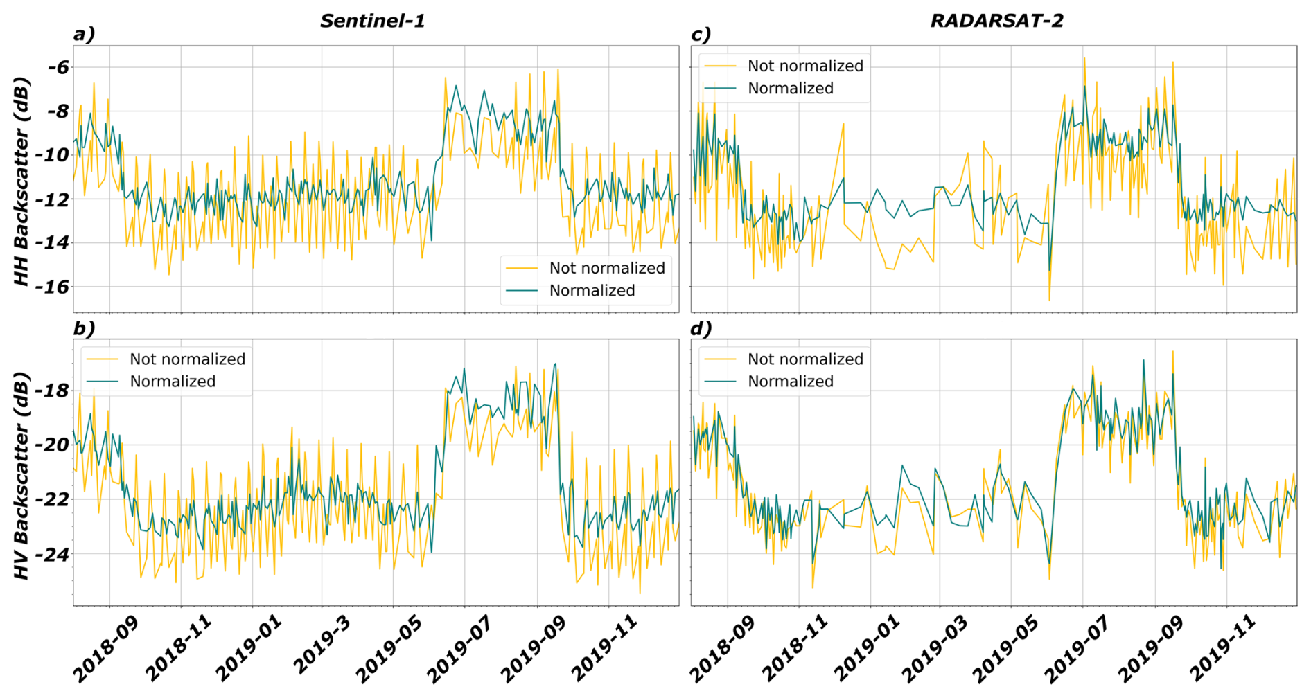
Figure 4 Examples of the backscatter time series for one pixel of Sentinel-1 and RADARSAT-2 data for the study period after basic preprocessing (yellow) and incidence angle normalization (green).

4.2 F/T detection algorithm development

As mentioned earlier, we evaluated three different methods to deduce the seasonal reference value for the algorithm (Sect. 4.2.1). A threshold optimization was conducted from the calculation of accuracy for increments of threshold between 0 and 1 (Sect. 4.2.2).

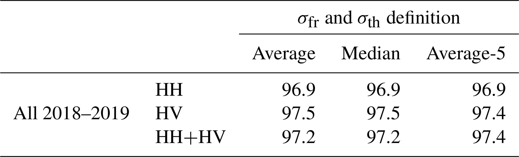
4.2.1 Comparison of the σ_fr and σ_th reference value

The two reference values σ_fr and σ_th were calculated independently for each of the reference sites. Table 3 shows that for the combination of the reference sites, the performance of the algorithm is not impacted by the approach used to determine the reference values over the complete study period, with a difference of less than 0.5 % in detection accuracy. The same similarities were observed when calculating the accuracy per transition season for each reference value method. Those similarities between methods confirm that C-band signal can easily discern the two thermodynamic stages of the soil independently from the method chosen. Even though we observed close to no difference, the “average-5” method could be more sensitive to the presence of residual noise or outlier backscatter measurements left in the time series, just as the “average” method could be. Therefore, we used the “median” method for the following analysis.

Table 3 Multisensor F/T detection highest accuracy (%) calculated with T_soil reference data, for the three reference values definitions of σ_fr and σ_th for the time series of 2018 to 2019.

4.2.2 Threshold optimization

Figure 5 shows the accuracy of the detection algorithm as a function of the threshold between 0 and 1 (at a 0.01 increment) on HH, HV and HH+HV datasets. The accuracy is calculated for the ten reference sites combined, with T_soil (solid line) and T_air (dashed line) reference values over (a) the entire time series; (b) the freezing transition periods for 2018 and 2019 combined; and (c) the thawing transitions for 2019. The algorithm applied over the entire time series (Fig. 5a) suggests high accuracy (>95 %) for threshold values ranging between 0.40 and 0.65 for all polarizations and temperature datasets. Figure 5b and c show the difference in the retrieval accuracy along the increment of thresholds during the freezing (11 August to 10 October 2018) and thawing (11 May to 10 July 2019) periods respectively. Results show that a clear threshold value maximizing the accuracy exists between 0.50 and 0.65 for the classification of the freezing period (Fig. 5b) for all datasets. For the thawing transition, multiple threshold values across a larger range yield a high accuracy (Fig. 5c).

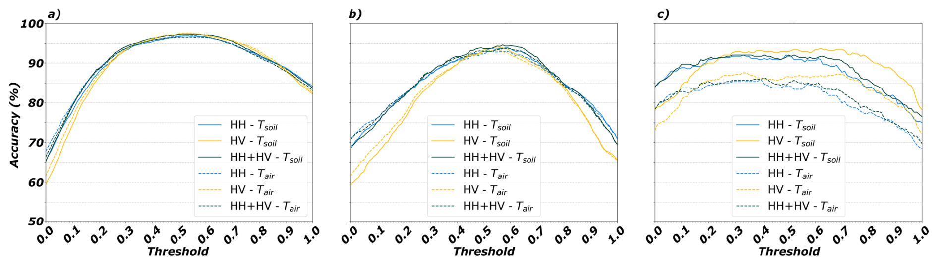
Figure 5 Accuracy of the seasonal algorithm over 0.01 increments on the threshold for (a) the entire time series of 2018 to 2019, (b) the freezing transition of 2018 and 2019, and (c) the thawing transition of 2019.

The signal classification during the thawing transition is largely insensitive to the threshold over a wide range of increments, where the accuracy remains mostly stable (0.2 to 0.6 for HH, 0.3 to 0.7 for HV and 0.2 to 0.7 for HH+HV polarization). A common threshold for both transition periods could then be considered for the surface F/T detection. Figure 5c also suggests that in the classification accuracy, the soil temperature performs better by almost 10 % when compared to air temperature over the range of thresholds presented. We therefore chose the optimized threshold from the best accuracy compared to T_soil measurements for the combination of both transition seasons. A threshold of 0.56 was defined as maximizing the accuracy of transition seasons for HH polarization and of 0.53 for HV polarization (Table 4).

Table 4 Accuracy for the combined transition period (F-2018, S-2019 and F-2019) with optimized threshold.

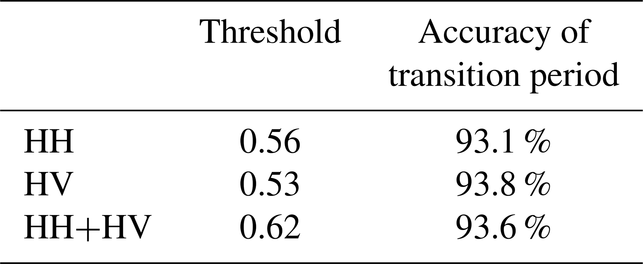
Since both polarizations show similar accuracy results for the F/T detection, the combination of the two polarizations also gives similar high results. The same threshold optimization was done on the Total H power time series and a threshold of 0.62 was found to optimize the accuracy of detection (Table 4).

4.3 Case study: impact of ecotype on surface F/T for a low arctic environment

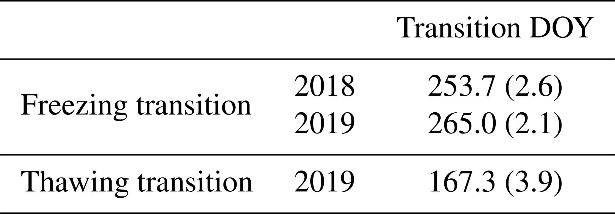
We created surface F/T maps with the optimized threshold of 0.62 using the Total H power over the three transition seasons, yielding three maps (Fig. 6) for the IMA+, one for each transition season. Depending on the transition season, between 74 % and 81 % of the original area appear in those maps after applying the masks (see Sect. 3.3). Table 5 shows the mean DOY for freezing and thawing transition seasons from 2018 and 2019 with the standard deviation calculated from the maps. For average DOY detected, S-2019 shows a higher standard deviation than F-2018 and F-2019. Overall, we can see that in 2019, the soil froze around 10 d later than in 2018.

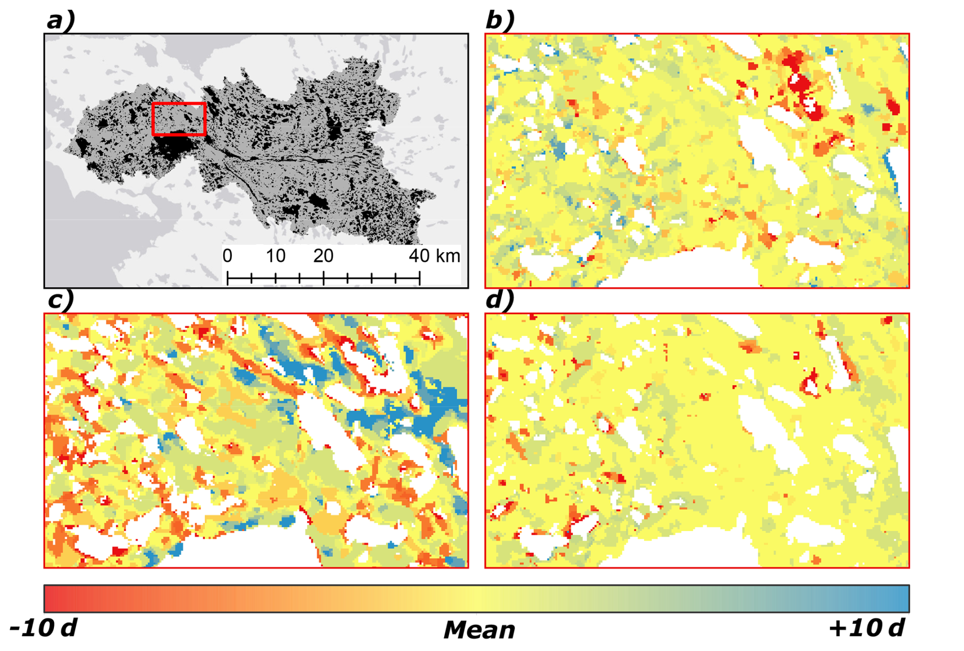
Figure 6 F/T map extent in red (a) with freeze and thaw DOY maps for the IMA + area using HH+HV for F-2018 (b), S-2019 (c) and F-2019 (d). Areas without data appear in white. The ecotype data extent for the Greiner Lake watershed is shown in (b) with the F/T map extent in red.

Table 5 Mean transition day of year (DOY) for the IMA+ with standard deviation in brackets for the three transition seasons.

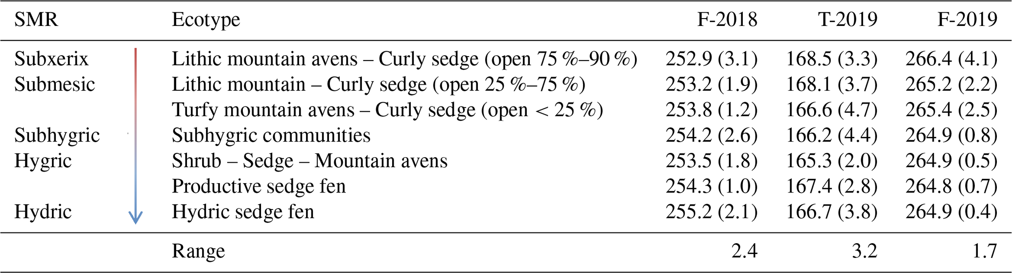
We investigated potential relationships between surface F/T DOYs and ecotypes, given that different ecotypes have different soil and vegetation moisture levels (i.e., thermal conductivity) implying consequences on the surface F/T cycles. Table 6 shows the mean and standard deviation of freezing and thawing DOY defined with HH+HV over the three transition seasons per ecotype class. The range, which is quite small for all seasons, represents the difference between the mean surface F/T DOY of the first and the last ecotype to transition for each season.

Table 6 Mean and standard deviation of surface F/T DOY for each ecotype class using Total H power (HH+HV) for the three transition seasons. Ecotypes appear according to their soil moisture regime (SMR) from subxeric to hydric (i.e., dry to wet).

Three GLS models were created to establish if a statistical difference exists between the surface F/T DOY of each ecotype classes per transition seasons. Figure 7 shows the model estimates values for freezing (Fig. 7a and c) and thawing (Fig. 7b) transition seasons along with standard deviation. For F-2018, drier ecotypes tend to freeze sooner than hydric ecotypes, and for F-2019, only the class Lithic Mountain avens – Curly sedge (Open 75 %–90 %) shows no overlap with the other classes. For the thawing transition season for 2019 (Fig. 7b), no clear trend is visible between the ecotypes but there is a clear difference between Lithic mountain – Curly sedge (Open 25 %–75 %) and Lithic Mountain avens – Curly sedge (Open 75 %–90 %) when compared with the other classes. Those drier and lower vegetation ecotypes (5 cm typical vegetation height) thaw later than the other more hydric and higher vegetation ecotypes (30 cm typical vegetation height).

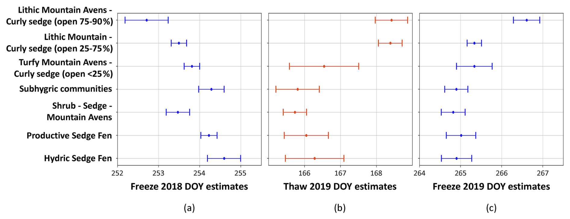
Figure 7 Estimated transition DOY from GLS models for 2018 freezing (a), 2019 thawing (b), and 2019 freezing (c) seasons with standard deviation per ecotypes classes.

5 Discussion

This study combined C-band SAR observations from Sentinel-1 and RADARSAT-2 sensors to create a quasi-daily time series, which delivers a spatially detailed surface F/T detection capacity and precision across an arctic tundra environment. The seasonal threshold algorithm was effective in classifying SAR backscatter observation into frozen or thawed states, with obtained overall detection accuracy of over 96 % for the whole time series, and over 91 % for every transition period. These results are similar, or even superior to other studies using SAR observations for FT monitoring in permafrost regions (Bartsch et al., 2025; Wang et al., 2022; Taghavi-Bayat et al., 2024). The influence of the snow cover on the freezing transition and the differences between the freezing and thawing detection ability are now discussed, along with the impact of the low arctic environment ecotypes on the transition onset for the case study region.

5.1 Evaluation of the seasonal F/T algorithm

5.1.1 Impact of snow on freezing transition

The temporal evolution of T_soil for the reference sites is quite different for F-2018 and F-2019 due to different meteorological conditions during those freezing transitions. Figure 8a and b show the temporal evolution of T_soil at two locations (IP8 and IP13) along with T_air. We chose the site IP8 and IP13 to illustrate the difference between moist and dry ecotypes respectively. The site IP8 is composed of a Sedge fen ecotype, which is a hydric ecosystem characterized as very moist to wet (McLennan et al., 2018). The clear zero-curtain effect in higher moisture ecotype is highlighted during F-2018 in IP8 (Sedge fen), with the soil temperature remaining close to 0 °C over a longer period, before freezing completely (Domine et al., 2018a). This is different compared to the drier IP13 site located in the Unvegetated (open >99 %) ecotype. In addition to the difference due to soil moisture, we examined snow cover information from the IMS Daily Northern Hemisphere Snow and Ice Analysis (U.S. National Ice Center, 2008). This dataset provides information at 1 km to determine the snow onset (>40 % coverage of 1 km) for these two transition seasons. We found that snow arrived almost one month later in 2019 (9 October 2019) than in 2018 (11 September 2018). The zero-curtain period is increased when snow covers the ground and isolates the soil from the cold air temperatures (Yi et al., 2019). We observed this with the soil temperature of the Sedge fen ecotype during F-2018 (Fig. 8a) when compared to the same location during F-2019 (Fig. 8b). On the other hand, the absence of snow cover increases cooling of the soil from the air, leading to a more direct freeze for both ecotypes (Fig. 8b). This is illustrated in Fig. 8b, when both i-Buttons freeze concurrently with T_air falling below freezing in F-2019. A clearer distinction between states is reflected in the C-band signal with a faster and greater decrease of backscatter between thawed and frozen soil in the F-2019 time series for both the Sedge fen and the unvegetated ecotype as shown in Fig. 8d compared to Fig. 8c. Interestingly, despite the difference in the soil moisture regime between the two sites, the backscattering trends are similar, with slightly higher σ⁰ at IP13 in winter, probably related to the lower fraction of ice in the soil. These results show a possible impact of summer water balance and soil moisture at the end of the season on the initial backscattering coefficient at the beginning of the freezing season. Our results show that even if the initial soil moisture change the backscattering at the beginning of the freezing seasons, the contrast between frozen and thawed backscattering remain large enough to use the proposed simple thresholding approach. Another possible impact on freezing identification is the presence of vegetation (Cohen et al., 2024). However, vegetation high and biomass in our study site is low with limited impact on backscattering as shown from studies using ASCAT (Liu et al., 2023). Hence, if vegetation senescence in fall as an impact on backscattering, the effect is much lower than the soil FT processes as shown by the accuracy over 93 % obtained in this study.

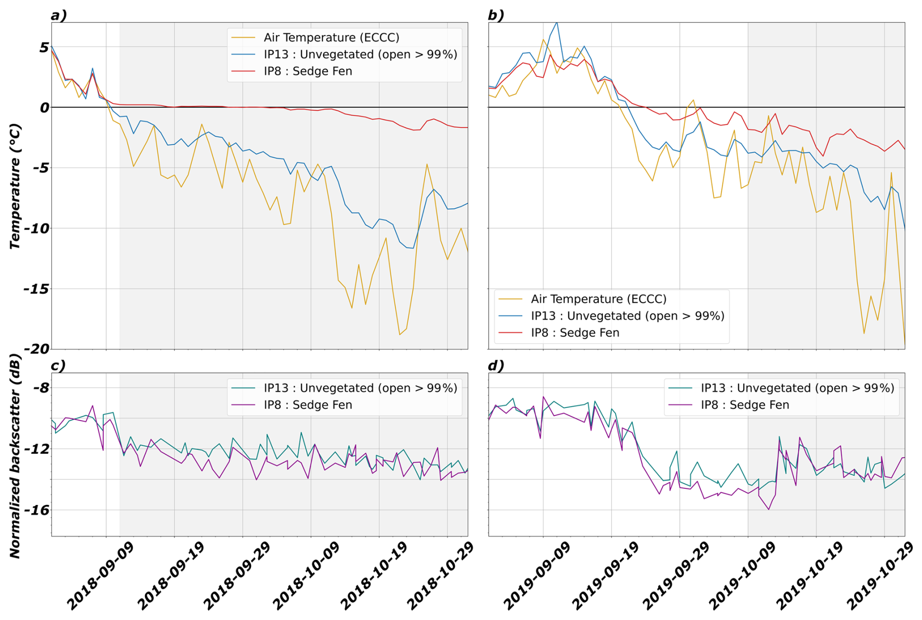
Figure 8 Surface soil temperature for two i-Buttons sites (IP8 and IP13) and air temperature (top) with HH+HV backscatter multisensor time series (bottom) for Sedge fen (IP8) site. Presence of snow on the ground is shown in grey for 2018 (left) and 2019 (right) freezing periods.

Furthermore, Fig. 8a shows that the decrease in the backscatter signal agrees with the start of the zero-curtain effect as measured at 2 cm in the soil. This result highlights that even though T_soil is not below zero, like for F-2018, the microwave signal decreases following the dielectric discontinuity of the soil surface when T_soil is close to 0 °C, as observed in Rowlandson et al. (2018), thus making the C-Band signal sensitive to the beginning of the zero curtain. Since the signal at C-band frequency is sensitive to the soil surface, we hypothesis that, at the beginning of the zero curtain and around 0 °C, a thin frozen layer (i.e., a change in the water phase) appears at the very top of the soil, creating a dielectric discontinuity and thus resulting in a backscatter decrease. Also, we chose the i-Buttons location to be representative of a homogeneous patch of land cover. However, the SAR pixels cover a soil surface of 2500 m². During F-2018, the start of the gradual backscatter decrease observed before T_soil reached 0 °C could be explained by the averaging of the soil contribution inside the pixels. Indeed, the punctual measurements of T_soil do not represent the full extent covered by the pixels especially when isolating snow is present on the ground, increasing the zero-curtain effect for higher ground moisture (Domine et al., 2018a).

As for the detection capacity of the algorithm, the faster decrease in the signal, showing a clearer distinction between surface states, resulted in higher accuracies for F-2019 classification (Fig. 9), meaning less uncertainty in the detection, than for F-2018 for every threshold increment. Nonetheless, the C-band signal was sensitive to the freezing onset of the surface with a decrease of 3–4 dB for the two fall seasons, with an accuracy higher than 93 % independently from the presence of snow compared to T_soil reference values.

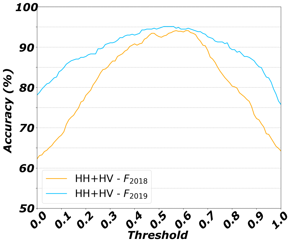
Figure 9 Accuracy, for every increment of threshold for HH+HV time series, for F-2018 and F-2019 independently.

5.1.2 Difference between freeze and thaw detection accuracy

Dividing the signal into freezing and thawing transition seasons during the threshold optimization showed a clear difference between the signal behavior for those two seasons, linked to the different processes driving those transitions. Regardless, Fig. 5b and c showed that we could use a common threshold definition for both transition seasons since, for the thawing classification, the accuracy is nearly independent from the change in threshold. This can be explained by the behavior of the signal during the thawing season, for which we observe a clear difference in backscatter between frozen and thawed surface. Generally, it is expected that the surface thaw onset happening under wet snow would be difficult to monitor, because wet snow is mostly opaque to microwave (i.e., surface scattering) (Ulaby et al., 1986). The dielectric properties of snow are defined in two distinct phases: (1) dry snow, having a low dielectric constant related to the absence of liquid water within it; and (2) wet snow, having a high dielectric constant related to the presence of liquid water in the air-ice mixture (Langlois et al., 2007). On one hand, the impact of snow depth in the winter season when the snow is dry should be minimal on C-band backscatter. Studies showed that C-band was not able to capture snow depth variations lower than 1 m (Lievens et al., 2019; Hoppinen et al., 2024). Snow depth observations performed by our group between 2015 and 2019 showed that maximum snow depth maximum reach around 0.35 cm (±0.17 cm) (Meloche et al., 2022), which limit the possible impact of dry snow on backscattering signal. On the other hand, the C-band signal would then decrease with the presence of wet snow on the ground (Tsai et al., 2019), which decreases the penetration depth and increases the surface scattering of the air and snow interface as air temperatures rise above zero in the spring. In fact, in the SAR temporal series, the backscattering coefficient decreases when air temperature rises above 0 °C. However, that decrease is rather small because the backscatter of frozen tundra soil is already low. This signal intensity decrease is followed by a sharp increase of the order of 3–5 dB related to ground surface thawing. Hence, the increase in T_air during spring matches the start of snowmelt. However, our results show a strong agreement of this increase with soil temperature rising above 0 °C, suggesting that the sharp backscatter increase is an indication of wet snow turning into exposed thawed soil. Even though the C-band signal is affected by the presence of wet snow on the ground (Cohen et al., 2024), the fact that the wet snow signal and the thawed soil seem to happen almost at the same time, could indicate that the detection of soil surface thawing during the spring using C-band SAR observations is possible considering the strong agreements obtained with the soil surface temperature in the Arctic's tundra environment. Nevertheless, to fully understand the thawing signal in such environment, the use of a more comprehensive dataset that include snow depth, snow temperature and snow liquid water content for different conditions (years and area) would be necessary. Studies using ground-based radar could also help to better understand the processes leading to the thawing signal in spring for arctic environments (King et al., 2018; Rowlandson et al., 2018).

5.2 Case study: Ecotypes effects on F/T DOY

The Total H power allows removal of the polarization dependency of the signal to the target. The modelled differences between ecotypes classes for the three transition seasons would therefore be due to the impact of different ecotypes on the surface thermal regime.

Freeze DOY. As discussed in Sect. 5.1.1, the presence of snow on the ground increased the zero curtain during fall. It creates a bigger gap between freezing DOY from different moisture level soil during F-2018, and in contrast, the absence of snow on the ground during F-2019 leads to a more homogeneous freeze across all ecotypes (Table 6) as detected. The estimated value from the GLS models for the F-2019 dataset shows that the difference between classes is not significant for almost all classes, except for the class Lithic mountain avens – Curly sedge (Open 75 %–90 %). Once again, considering the sensitivity of the signal to the water phase change at the soil surface, those similarities could be linked to the absence of snow on the ground, making the soil surface more sensitive to the cooling of air temperature, regardless of the soil moisture level or ecotype. For F-2018, as shown earlier in Fig. 7a, the difference between ecotype in freezing DOY is strongly linked to the moisture level of the soil. As discussed earlier, a higher soil moisture tends to freeze later than a drier soil due to the presence of more latent heat linked to the presence of water, and this difference is increased by the presence of an insulating snowcover.

Thaw DOY. For the thawing transition, the model estimated that drier ecotypes with lower vegetation thaw later than ecotypes with higher moisture and vegetation. Higher vegetation increases trapping of the snow, resulting in deeper snow cover (Sturm et al., 2001, 2005) which insulates the ground more effectively from the cooling of the air. Furthermore, the presence of higher vegetation increases the creation of depth hoar, which is an even more insulative snow cover (Domine et al., 2016). Sturm et al. (2005) suggested that deeper snow cover result in higher soil temperature throughout winter. Moreover, Domine et al. (2022) found that the branches buried in the snow cover absorb solar radiation under the snow and conduct heat to the ground, resulting in earlier thaw for vegetated areas. That could explain the faster thaw observed for higher vegetation ecotypes. We could then hypothesize that the difference observed in the thawing DOY is linked to vegetation thermal effect.

The small but significant differences of 2–3 d in Freeze DOY and Thaw DOY shows the importance to get high spatial near-daily FT maps to monitor the impact of FT cycles on ecosystems processes in Arctic environments. Indeed, because the growing seasons is short in these environments, few days in FT timing can have important impact on ecosystems processes. For example, Gehrmann et al. (2022) showed that a delayed senescence by 3.5 d can lead to an extension of the growing season end of 10 % for certain species in Arctic environments. The precise detection of the soil freezing and thawing is also important for accurate monitoring of soil carbon emissions (Arndt et al., 2022; Mavrovic et al., 2023).

6 Conclusion

In this study, we applied C-band SAR data from multiple sensors to develop an algorithm to estimate freezing and thawing onset of the soil surface in an arctic environment near Cambridge Bay, NU. To analyze the potential of C-band SAR quasi-daily time series for soil surface F/T onset detection in the low arctic tundra, we used the seasonal threshold algorithm defined in Derksen et al. (2017) and Rautiainen et al. (2016) with an optimized threshold. As a case study, we then evaluated the impact of ecotypes on the surface F/T DOY onset across the study site by comparing the surface F/T maps created from the Total H power (i.e., HH+HV) time series to ecotypes maps created by McLennan et al. (2018).

Normalizing the incidence angle of the signal for both sensors helped to minimize noise in time series that combines multiple orbits of observation, and therefore provides an improved distinction between soil states. Likewise preprocessing the Sentinel-1 and RADARSAT-2 imagery allowed to combine the two datasets to create a multisensor time series with a revisit time of just above 1 d for the key transition seasons of late 2018 and 2019. Since earlier studies have already suggested the spatial heterogeneity of the soil F/T, we had hypothesized that the spatial resolution (i.e., 50 m×50 m) of the SAR imagery would notably improve the retrieval of the spatial variability for the F/T onset transition when compared to passive microwave approaches. Parameterizing the seasonal threshold algorithm using T_soil reference data from multiple sites produced an overall detection accuracy of over 96 % for the whole time series, and over 91 % for every transition period. To create surface F/T onset maps of the IMA+, we used the threshold defined with the accuracy optimization on surface T_soil for the reference sites. Giving that soil type, moisture level and vegetation height directly impact the soil thermal regime, we hypothesized that the ecotype classes influence the soil surface F/T onset according to their characteristics. Results from the coupling of the surface F/T DOY maps with the ecotypes maps showed that differences between some ecotype classes are linked to moisture levels during freezing and to the presence of vegetation during thawing.

Overall, this study demonstrated the capacity of C-band SAR backscatter intensity to detect surface F/T in the tundra environment. The multisensore approach allowed to create high spatial resolution near-daily FT product based on SAR observations allowing to better monitor ecosystem processes in Artic environments but could also help mitigate potential satellite failure and increase our capacity to produce long-term SAR FT products. Note that the signal of wet snow limits accurate thawing transition detection. For future use of the algorithm, backscatter reference values (σ_fr and σ_th) used inside the seasonal threshold algorithm could be updated by adding the new data for each year to decrease the impact of individual seasons. Also, average snow depth per ecotypes could help to validate if the retrieved thaw DOY is more linked to the presence of vegetation or snow cover. The surface F/T product created from this study demonstrates how, on one hand, the SAR backscatter can be used for surface F/T detection in low vegetation and shallow snow-covered terrain (Meloche et al., 2022), and on the other hand, how it could be used as complementary data to improve modelling of the soil thermal regime.