the Creative Commons Attribution 4.0 License.
the Creative Commons Attribution 4.0 License.
 | 03 Jun 2026
Learning to melt: Emulating Greenland surface melt from a polar RCM with machine learning
Sebastian Scher
Ruth H. Mottram
Peter L. Langen
Predicting surface melt on the Greenland ice sheet is critical for understanding surface mass balance (SMB) and its sensitivity to a changing climate. Polar regional climate models (RCMs) are the primary tools for simulating melt and projecting future SMB, but different models produce significantly different results. However, they are too computationally expensive to create the large ensembles needed to quantify this uncertainty. We develop a neural network based emulator that predicts daily surface melt from atmospheric variables, trained on output from the polar RCM HIRHAM5 and its firn model DMIHH forced by ERA-Interim. The emulator uses a physics-informed design combining short-term weather with long-term climate memory, capturing both immediate atmospheric forcing and accumulated firn characteristics. Input selection study shows that turbulent heat fluxes, downwelling radiation, and precipitation together with seasonal encoding suffice to reproduce surface melt. The emulator achieves mean absolute error below 0.21 mm w.e. per day relative to the surface melt produced by DMIHH across all six Greenland drainage basins, with the errors primarily attributable to spatial over-smoothing. Our work demonstrates that machine learning can successfully emulate firn model behavior from climate forcing alone with computational costs orders of magnitude lower than traditional simulations. Once retrained for specific climate forcings, the emulator thus enables extensive ensemble projections. Furthermore, the modular architecture can be readily adapted to emulate other SMB quantities such as runoff. This represents a crucial first step toward computationally efficient emulation of polar regional climate models and surrogate modeling of SMB components in Earth system modeling.
- Article
(11481 KB) - Full-text XML
- BibTeX
- EndNote


The Greenland ice sheet (GrIS) is losing mass today, and it will continue to do so in the future. Runoff caused by surface melt is a key component of surface mass balance (SMB), with increased melt leading to a negative SMB and subsequently a decrease in mass. With ongoing atmospheric warming and the positive feedback of surface melt with albedo and the lowering of elevation, surface melt will increase further in the future (Meredith et al., 2019). While future projections agree that melt will increase, the predictions are inconsistent about the rate of this melt increase and associated SMB loss (Glaude et al., 2024).
Polar regional climate models (RCMs) combined with a firn model show the best agreement with observational data among different modeling approaches for predicting SMB (Fettweis et al., 2020). But they are also the most complex and computationally intensive approach, as they require running two numerical models: (a) the RCM to downscale atmospheric data from a forcing global climate model (GCM), and (b) the firn model to infer surface mass balance based on the surface energy balance (SEB) and firn properties that evolve from local atmospheric conditions. Both models are based on physical processes, modeled with computationally expensive numerical schemes. Despite their common framework, polar RCMs such as HIRHAM (Mottram et al., 2017; Langen et al., 2017), MAR (Fettweis et al., 2013, 2017), and RACMO (Noël et al., 2018) differ considerably in their assumptions, physical process representations, parameterizations, and numerical schemes, producing notable discrepancies in their SMB estimates (Fettweis et al., 2020). These discrepancies increase even more in future scenarios, as the models exhibit different sensitivities to atmospheric warming, leading to a varying increase in melt water production, and in turn to a positive feedback amplifying the models' discrepancies even more (Glaude et al., 2024). The use of a diverse ensemble of simulations is therefore crucial to mitigate model-specific biases and to improve robustness and reliability of projections, as well as to evaluate the projections statistically (Glaude et al., 2024; Mankin et al., 2020). However, the high computational costs of polar RCMs limit the generation of large ensembles.
In recent years, Machine Learning (ML) has shown great prospects for simulating various parts of the Earth system (Pan et al., 2025; de Burgh-Day and Leeuwenburg, 2023; Reichstein et al., 2019). ML-based emulators of climate model output are data-driven approximations of complex physical models that can produce predictions at a fraction of the computational cost of the respective physical models, allowing for the production of large ensembles (Tebaldi et al., 2025). More specifically, an emulator of a polar RCM could be used to extend existing simulations over longer time periods, to complement projections under various Shared Socio-economic Pathway (SSP) scenarios which were not covered by the original simulations, or to produce simulations under new climate forcings. Additionally, emulators can be used not only for creating more simulations, but also for rapid hypothesis testing and sensitivity analysis. Moreover, besides emulating Earth system components standalone, ML emulators can also be used for surrogate modeling within numerical Earth system models.
ML applications for firn and SMB modeling include approximating observational data using reanalysis climate data (Vandecrux et al., 2024; Ogunmolasuyi et al., 2025; Bolibar et al., 2020; Anilkumar et al., 2023), improving model estimates by observational data (Hu et al., 2021; de Roda Husman et al., 2024), or emulating firn model outputs (Sellevold and Vizcaino, 2021; Veldhuijsen et al., 2025; van der Meer et al., 2023; Dunmire et al., 2024). These studies predominantly employ tree-based methods like XGBoost, which builds an ensemble of decision trees where each successive tree corrects errors from previous ones (Chen and Guestrin, 2016), or neural networks (NNs), which stack nonlinear transformations to approximate complex functions (Goodfellow et al., 2016). While XGBoost offers simpler deployment, NNs can achieve superior performance given sufficient training data and careful tuning (Tyralis et al., 2021; Wesselkamp et al., 2025).
Furthermore, ML techniques for image super-resolution methods that reconstruct high-resolution images from low-resolution counterparts have been adapted for downscaling meteorological variables (Sun et al., 2024; Hadjipetrou, 2026). de Roda Husman et al. (2024) uses such a ML downscaling approach to downscale SMB to a higher spatial resolution, while van der Meer et al. (2023) infers SMB directly from coarser-resolution climate fields at a coarser resolution, effectively emulating both the RCM and the firn model, simultaneously. While this approach delivers SMB estimates directly from GCM data without intermediate climate downscaling, separating these processes offers key advantages. Downscaling is inherently spatial, requiring models to capture atmospheric dynamics and topographic effects, whereas firn models operate on one-dimensional vertical columns. A standalone firn emulator trained on local atmospheric forcing learns location-agnostic relationships that generalize across different locations and climate states, rather than encoding spatial patterns specific to the training domain. This design enhances robustness, since unusual melt events triggered by specific atmospheric conditions can be predicted even at atypical locations if similar conditions occurred elsewhere in the training data.
Existing works operate at annual or monthly timescales and use only the current timestamp data for regression, with only Veldhuijsen et al. (2025) and Vandecrux et al. (2024) incorporating multi-scale temporal aggregation to capture slow-evolving firn properties. However, the temporal history required for daily melt predictions remains unexplored. Firn properties integrate conditions over years to decades, whereas surface melt responds to daily atmospheric forcing but also evolves gradually, suggesting temporal history is necessary. Additionally, most approaches rely on air temperature as a melt proxy rather than direct physical drivers of the surface energy balance, i.e., turbulent heat fluxes and radiation, even though these variables are available in reanalysis products and polar RCMs.
In this study, we address these gaps by developing a NN for emulating GrIS surface melt, based on model output from the polar RCM HIRHAM5 (forced by ERA-Interim). We thereby focus on two key aspects that distinguish our approach from existing work: First, we operate at daily resolution, introducing new challenges due to the high temporal variability of surface melt compared to monthly or annually aggregated data. To address this, we design our NN in a physically informed way with separate modules, extracting short- and long-term information from daily and 10 year aggregated data separately. We systematically test the impact of including short-term history and long-term information, as well as configurations including albedo or the previous day's melt. Second, we expand the range of input variables compared to previous studies. Contrary to most existing work which rely primarily on air temperature and precipitation data, we also include the direct drivers of the SEB. We then conduct a systematic input selection analysis to assess the impact of including atmospheric variables beyond the direct SEB drivers, as well as seasonal information. We find that snowfall, rainfall, and seasonality are important predictors in addition to the direct SEB terms, while including air temperature does not increase model performance any further.
This work is a first step toward comprehensive emulation of SMB processes in polar RCMs, with surface melt being a key component of GrIS SMB. While our location-agnostic architecture is applicable to different polar RCMs and future scenarios, application requires validation under data distribution shift and potential retraining on the respective RCM outputs, which we identify as important next steps. We demonstrate that our NN accurately reproduces daily melt patterns across the whole GrIS, while requiring only approximately one minute of computation per year on a single CPU, demonstrating that emulators can match physical model accuracy at a fraction of the computational cost.
2.1 Data
For the creation of our emulator we use daily output of the polar RCM HIRHAM5 with its firn model DMIHH, forced by ERA-Interim for the period 1980–2016 taken from Langen et al. (2017). We first describe the HIRHAM5-DMIHH simulation data to understand its internal consistency and the physical relationships it builds upon, which motivates the design of our NN and the systematic input selection study performed in this work. Thereafter, we describe the data cleaning and processing for training the NN.
2.1.1 HIRHAM5-DMIHH simulation data
In Langen et al. (2017), HIRHAM5 is run at a spatial resolution of 0.05°×0.05°, with a snow layer of and an internal albedo parameterization dependent on surface temperature, to determine the energy and moisture flux interactions at and below the surface (Lucas-Picher et al., 2012). The resulting atmospheric fields are then used to force the firn model DMIHH offline.
DMIHH is a one dimensional model organized in 32 layers totaling of firn. HIRHAM5 mass fluxes (snowfall, rainfall, deposition, sublimation), downwelling shortwave and longwave radiation (SW↓, LW↓), and latent and sensible heat fluxes (LHF, SHF) update DMIHH hourly at the surface. The surface state is determined via the SEB, with surface temperature being bound above by 0 °C, and any excess energy producing surface melt:
where GHF is the ground heat flux from the layers below, and LW↑ the upwelling longwave radiation depending on the surface temperature. The surface albedo α is calculated internally based on surface temperature and snow depth, with α=0.85 for cold snow, decreasing to 0.65 as the surface warms toward the melting point, and dropping further as surface snow diminishes, with α=0.4 at lowest for bare ice exposure (i.e., zero snow fraction in the surface layer). While snowfall and rainfall are not directly part of the SEB, they have an indirect influence via the albedo: rainfall is simulated with a temperature of 0 °C and thus warm the surface if its below the melting point; snowfall increases albedo if snow depth is low. The firn model runs offline, which means that atmospheric data applies forcing to the surface without feedback from the surface back to the atmosphere. Consequently, the latent and sensible heat fluxes are prescribed by the RCM without adjustment for actual surface characteristics.
The firn pack in the DMIHH simulation was spun up by repeatedly cycling 1980–1989 until decadal means of runoff and subsurface temperatures reached a steady state, then run continuously for 1980–2016, with daily aggregated SMB outputs and their associated driving HIRHAM5 outputs saved for the full period. This temporal aggregation potentially constrains melt emulation accuracy by smoothing sub-daily variability and short-lived extremes that control timing and peak rates of melt. However, daily resolution enables broader utility in future applications, aligning with the typical daily temporal resolution of both GCM and RCM output, as well as current ML downscaling approaches.
2.1.2 Data cleaning
Although data from physical simulations are generally consistent, they may still contain extreme values and outliers caused by numerical instabilities, although these are very rare. While these individual outliers do not affect the overall assessment of modeled melt or other properties, they can disproportionately influence gradient-based optimization, distort the loss function, and impair stable convergence during ML model training. In order to decide how to treat these extreme values and outliers we must consider their source, their impact, and relation to other variables.
Aggregating rainfall and snowfall to daily values during postprocessing, some negative rainfall values arise as numerical artifacts. We set these values to zero for consistency. Furthermore, rainfall and snowfall show some suspiciously high values of up to about 700 and 1000 mm w.e. per day, respectively. Although they are likely caused by numerical instabilities in high relief topography, we do not correct these values to preserve consistency between the precipitation and the firn model output data used as target. However, we transform both rainfall and snowfall data by applying the logarithm (after adding 1, ensuring the transformation is well-defined for 0 values), which compresses these very high values. While this transformation neither adds nor removes information, it improves the data's usability for ML model training by preventing small values from vanishing in numerical noise relative to large outliers.
In rare instances, numerical instabilities also produce events of surface temperature runaway, leading to unrealistic surface temperatures approaching 0 K due to excessive surface cooling from sensible heat flux as low as −400 W m−2. We correct these heat flux values to a lower bound of −140 W m−2, which was the lowest sensible heat flux observed in simulations unaffected by the runaway. The ranges for sensible and latent heat flux span several hundred watts per square meter, yet the majority of the data are concentrated in a very narrow range. To expand the narrow and compress the large ranges, we transform heat flux values x with a symmetric logarithm transformation according to Webber (2013), with λ=5 for LHF and λ=15 for SHF, corresponding to approximately half of their respective inter-quartile ranges.
2.1.3 Data preparation for training
For training a ML model we need a data set to train the model (training set), a dataset to monitor the progress during training and guide decisions during model development (validation set), and an until then unseen set for the final model evaluation (test set). When splitting data, internal dependence structures (e.g., temporal or spatial autocorrelation, data grouping/clustering) together with the modeling task need to be considered to avoid information leakage into the training set (Auffarth, 2021; Roberts et al., 2017). For temporally structured data, this necessitates splitting along the time dimension in contiguous blocks (e.g., entire years) rather than individual samples (e.g., single days) to preserve temporal independence and ensure the validation and test sets remain truly distinct from the training set.
We split the data spanning from 1980 to 2016 into the three separate periods: a training period (1990–2013), a validation period (2014), and a test period (2016). The first 10 years of data (1980–1989) are included indirectly in the training set as decadal averages for the long-term module. To prevent information leakage between training and final evaluation, we introduced a one year gap between the validation and the test period, which is a common strategy for evaluating models using data with a structural dependency (Géron, 2019; Roberts et al., 2017). Although the time windows for calculating the decadal mean conditions still overlap, this overlap is considered to have negligible impact on the validity of the tests because this study focuses on a relatively short period lacking significant trends. Therefore, the decadal means primarily capture location specific characteristics rather than temporal development.
Our data split prioritizes maximizing the training set to expose the model to a broad range of atmospheric conditions and interannual variability. Consequently, we allocated only single years for validation (2014) and test (2016) periods. While the representativeness of the test set is important to report unbiased final model performance, the representativeness of the validation set is important to make fair decision during model development. Expanding either set to two or three years would reduce training data without guaranteeing improved representativeness. To mitigate potential bias from using single-year periods, we instead verified that both 2014 and 2016 were non-anomalous years in terms of total melt extent (Appendix A).
For a model to successfully learn a specific task, we need not only a big quantity of data, but sufficient quantity of data that is actually relevant for the specific task we aim to solve. The spatial resolution of 0.05°×0.05° results in 58 391 grid cells for the GrIS, and thus just as many samples for every single day in the data set. While selecting a long training period of 23 years ensures large interannual variability in the training set, not all of this data contains information that is relevant for solving our task, since surface melt is zero, or very close to zero, for large areas of the ice sheet and a substantial part of the year. Additionally, neighboring grid cells often exhibit very similar behavior, meaning that large spatial datasets can contain considerable redundancy with respect to the melt patterns relevant to model learning.
To reduce the portion of low-relevance data samples, we apply strategic sub-sampling in time and space. The temporal sub-sampling reduces the number of no/low melt days by randomly sampling 100 d per year from a normal distribution centered around the 24 July (as peak of the melt season) and a standard deviation of 60 d. The spatial sub-sampling, on the other hand, favors grid cells in high melt areas over dry areas by selecting 5000 grid-cells according to predefined zone specific probabilities (see Appendix B). By sub-sampling 5000 grid cells and 100 d per year from the training period, we create a training set of 12 million samples, reducing training costs significantly compared to the full data set of 511 million samples. While only about 6 % of the full training set show melt above 1 mm w.e. per day, the temporal and spatial sub-sampling increase this ratio to approximately 26 %. This sub-sampling stabilizes the training process; without it, the network tends to converge to the trivial local minimum of constantly predicting zero melt. We monitor training progress on the likewise sub-sampled validation set, but conduct model comparisons on the entire validation period data set to inform design choices, and report final performance on the entire test period data set.
As inputs for our NN, we select atmospheric variables that contribute directly to the SEB, as defined in Eq. (1), or indirectly: sensible heat flux SHF, latent heat flux LHF, downwelling longwave LW↓, downwelling shortwave radiation SW↓, rainfall R, snowfall S, and near-surface (2 m) air temperature T. We denote these input variables at daily resolution Xd. In addition, we include the cyclic features and (with DOY the day of year) to encode seasonality in our model. Lastly, long-term history is represented by aggregates of the input variables over the previous 10 year average, denoted by Xl. The target variable is daily surface melt. Since absorbed shortwave radiation is highly sensitive to surface albedo α, we also test model setups incorporating α. As a last preprocessing step, all the data is standard scaled to zero mean and unit variance with respect to the sub-sampled training data.
2.2 Emulator design
Since we aim to emulate surface melt modeled by the DMIHH firn model, we refer to that modeled surface melt as the “true” melt. The output of our ML model is called the “predicted” melt or “prediction”. With SM(t) denoting the true melt, and the predicted melt for a specific day t, we formulate our problem as finding a function f such that
for all days t, where Xd(𝒯) represents the daily input variables for N+1 d , Xl(t) the long-term inputs leading up to day t, and the melt prediction of the previous day.
Many approaches can yield an appropriate approximation function f, and there is a priori no single best algorithm. Rather, the choice depends on factors such as the type of the problem, the type and complexity of the data, as well as its quality and quantity available for training (Goodfellow et al., 2016; Wesselkamp et al., 2025). Given the highly nonlinear characteristics of the data set and the large amount of available data, we have chosen a NN for regressing the surface melt based on atmospheric variables (Anilkumar et al., 2023; Tyralis et al., 2021).
2.2.1 Neural Network Fundamentals
A NN is composed of k layers, which represents a concatenation of functions such that . Each fi takes the previous layer's outputs, combines them linearly, applies a nonlinear activation function, and passes the results forward to the next layer. The coefficients of these linear combinations are the parameters that are optimized during training of the NN. The output layer k yields the final prediction, while the previous layers are called the hidden layers. Each layer consists of neurons which represent the number of outputs of each function fi, and NN structures are often summarized by denoting the number of neurons of each (hidden) layer, e.g., a network with three layers containing 10 neurons each is written as “10-10-10” (Goodfellow et al., 2016). The hidden layers typically share the same non-linear activation function, e.g., Rectified Linear Unit (ReLU). We use LeakyReLU activation function in the hidden layers, a computationally efficient variant of ReLU that mitigates the drawbacks of classical ReLU (Dubey et al., 2022). The output layer often uses a different activation function than the hidden layers and is based on the task. Since our task is a regression task, we use no activation function. The whole network operates on scaled data; during inference the model predictions are reverse-scaled and clipped at zero to ensure non-negative melt predictions.
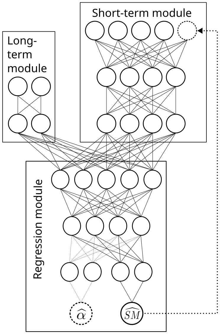
Figure 1Schematic of the modular neural network with short-term module, long-term module, and regression module to output , the additional output and the autoregressive element (dashed elements).
2.2.2 Network architecture
We designed the NN in three separate modules: two feature extraction modules and one regression module, as depicted in Fig. 1. The first extraction module, the short-term module, takes the daily inputs Xd of days as inputs to determine the current forcing on the surface layer. Furthermore, it incorporates the seasonal encodings for day t, intended to approximate the firn cold content through seasonal indicators.
The second module, the long-term module, uses the long-term inputs Xl. These long-term inputs are motivated by the spin-up procedure common to firn models and are meant to describe the prevailing firn characteristics at a site. We include these inputs alongside the seasonal encoding to provide location-specific information on firn cold content and bare-ice exposure proneness, which are factors that affect surface albedo and, consequently, surface melt.
The outputs of the two modules are then concatenated and fed into the final regression module which outputs the melt prediction for that day. While our proposed model configuration, Modular NN, consists of these three modules only, the network can be extended further by an autoregressive element, or by additional target variables. The autoregressive element (dashed arrow in Fig. 1) feeds the melt of the previous day back into the daily module of the network to include the self–enhancing effect of surface melt. Alternatively, we use albedo as additional target variable since simultaneously learning albedo might improve melt predictions (Cipolla et al., 2018; Sadler et al., 2022). In this case, Eq. (2) holds true not only for melt SM but simultaneously for albedo. While the weights of the NN f are shared for predicting melt and albedo throughout most of the network, the regression module branches before its final layer, with separate last hidden layers for the two output neurons predicting melt and albedo (indicated by the dashed neuron connections for albedo output in Fig. 1).
Given this network design described above, we develop our emulator in two stages. First, we optimize the network configuration while keeping the atmospheric input variables fixed. Then, using the best configuration, we study how using different subsets of atmospheric variables as inputs affect model performance by retraining on multiple variable subsets.
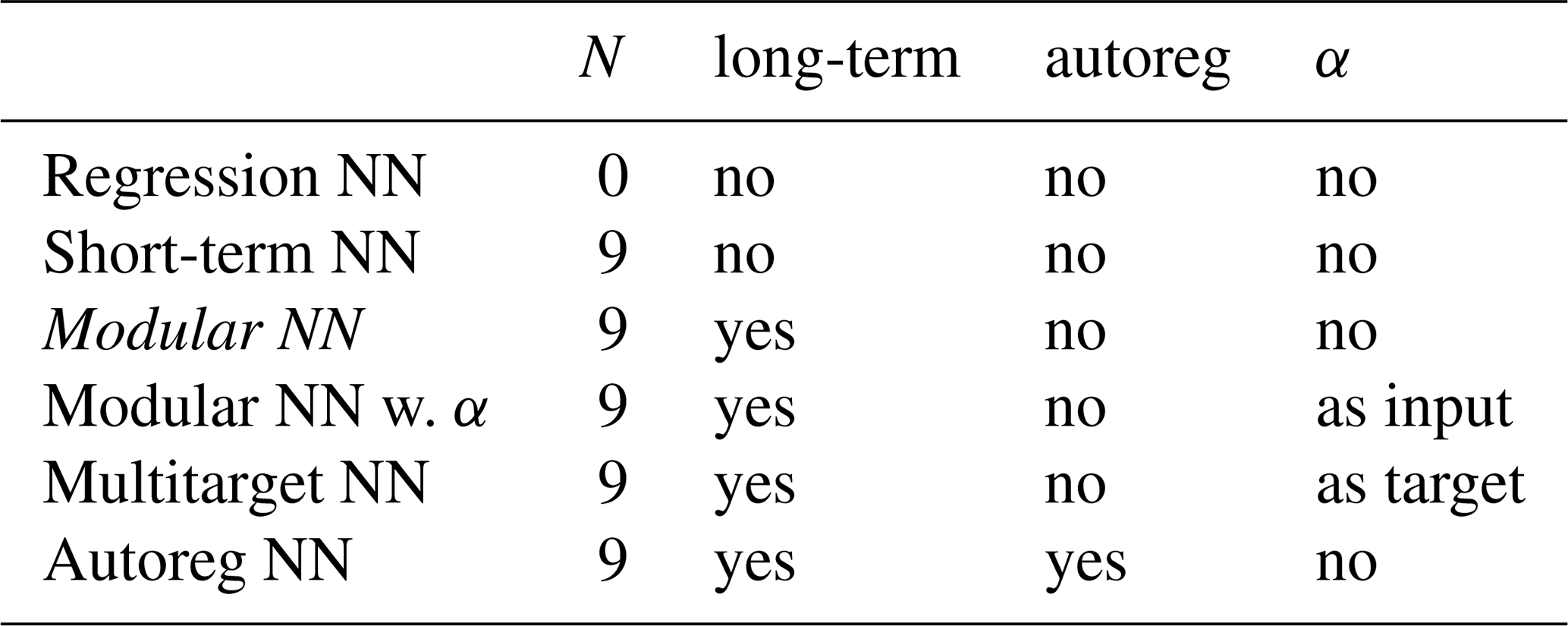
Table 1Overview of network configurations ordered by complexity, with their respective use of number of previous days N in the short-term module, the long-term module, α as additional target variable (Multitarget NN), and the autoregressive element (AutoregNN). Our main configuration Modular NN is indicated in italic. While Modular NN does not use α, we also trained a version of Modular NN with α as input as an upper benchmark for performance.
2.2.3 Network configuration study
To determine the necessary yet sufficient network modules and elements, we developed our configuration iteratively, by sequentially tuning the network configurations listed in Table 1. During this process we keep the atmospheric variables used for inputs fixed: As daily inputs Xd we use all the relevant atmospheric variables SHF, LHF, LW↓, SW↓, R, S, and T, together with the seasonal encoding. As proxy inputs for the long-term conditions Xl we use the 10 year averages of S and T.
The simplest configuration, Regression NN, consists only of the short-term module, using climate conditions of only the current day t as input (i.e. N=0), representing a pure regression model without any short-term or long-term historical information. This results in 9 input features (7 climate variables + 2 seasonal encoding variables), and we choose the hidden layers of the network to be 64-128-128-64-32-16-16, terminating in a single output neuron for melt prediction.
After having established this regression baseline, we investigate the impact of historical information by tuning Modular NN consisting of a short-term and a long-term module. The short-term module takes daily inputs from both the current and several previous days. The long-term module has two input neurons, and we choose two hidden layers of 32 neurons each. The hidden layers of the short-term module comprise 128-128-256, and the regression module combining the extracted feature from the two modules comprises 256-128-64-32-16-16. We tuned the number of the of preceding days and found that N=9 resulted in the best performance on the validation set. To investigate the necessity of the long-term module, we fix the number of past days at N=9 and tune the network without the long-term module (Short-term NN). This results in a network with 72 input features and hidden layers 128-128-256-256-128-64-32-16-16.
To investigate the impact of the surface albedo α, we train a configuration Modular NN w. α, where α is included in the daily inputs Xd. While this model cannot be used for firn emulation since α itself is an output of the firn model, this model serves as upper benchmark. In contrast, the model Multitarget NN does not use α as additional input but as additional target, so that the model can learn α and its impact on melt production. Multitarget NN results in two output neurons, one for melt and one for albedo. Next, we test whether incorporating an autoregressive step in the Modular NN improves model performance. Autoreg NN is thus also based on the configuration of Modular NN, but the melt of the previous day t−1 is used as additional input. Autoreg NN is tuned using the true previous melt as input during training (called teacher-forcing), although we also experimented with autoregressive learning approaches using the previous prediction directly during training. More details on the tuning process can be found in Appendix C.
2.2.4 Systematic input selection study
We perform a systematic input selection study on our identified best-performing configuration Modular NN. In ML, such studies are called input ablation or sequential input selection: input variables are iteratively added or removed (ablated), and model performance is assessed after retraining. This approach assesses the necessity of each input variable for solving the task, contrasting with post-hoc feature importance analyses (e.g., SHAP Lundberg and Lee, 2017) that evaluate how much a given feature contributes to an already trained model's prediction (Flora et al., 2024; Molina et al., 2023). The goal is to include all necessary variables while excluding redundant ones, as they inflate model complexity and can damage model performance, generalization, and interpretability. Finding the relevant features is not always straightforward and should not rely solely on feature correlation, but include domain knowledge (Theng and Bhoyar, 2024).
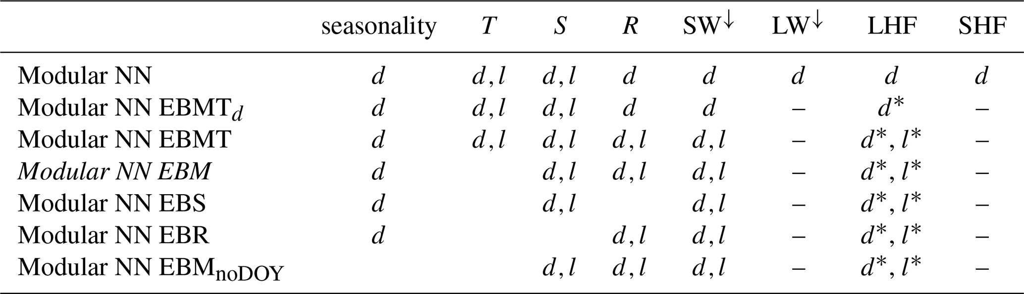
Since we know the direct drivers and mechanisms of melt production, i.e., the SEB terms according to Eq. (1), we can systematically aggregate and remove inputs based on domain knowledge. Our input selection study is summarized in Table 2, and is twofold: The first part is to sum up the energy input terms LW↓, LHF, and SHF, since they all contribute equally to the SEB. The NN needs only to learn from total energy input rather than the individual components, improving model robustness while reducing complexity. In contrast, SW↓ needs to be handled separately, because albedo strongly determines the energy finally absorbed by the surface. We define Modular NN EBMTd, which uses daily inputs of the energy balance variables EB (with LW↓, LHF, and SHF summed up, and SW↓ separate), the mass variables M (S and R), and the near-surface temperature T. The long-term inputs remain the same as in the default Modular NN (10 year averages of S and T).
The second part is a classical input selection study, sequentially adding and removing input variables. For this we start with a more extensive model, Modular NN EBMT, using all the atmospheric variables from the short-term module also in the long-term module. This allows us to determine the importance of long-term energy input rather than relying on temperature T as a proxy. We then sequentially remove variables: removing T yields Modular NN EBM (energy balance and mass terms only); removing R yields Modular NN EBS (energy balance and snowfall); removing S yields Modular NN EBR (energy balance and rainfall).
Table 2Overview of the input selection study: Modular NN with the inputs used in the configuration study serves as the baseline. With the network configuration fixed, we vary the atmospheric variables used as inputs. With d we indicate variables used in the short-term module, and l variables that are used as 10 year averages in the long-term module. The starred versions d* and l* indicate that the variables spanned by the line are summed up and provided as a single input to the model.
2.3 Emulator training
Each configuration is trained multiple times for 300 epochs, respectively, tuning the learning rate using the Python library Optuna (Akiba et al., 2019) for Bayesian optimization. We use Adam optimizer (Kingma and Ba, 2014), a batch size of 256, a learning rate decay factor of 0.9 every 50 epochs, and gradient clipping to a norm of 1 to stabilize training. For a more detailed description and the results of the tuning procedure, see Appendix C.
We performed the training on an NVIDIA GRID A100D-40C GPU with 16 vCPUs (128 GB RAM). Individual training runs required approximately 25–45 minutes, depending on the complexity of the configuration. While our network configurations are regarded small in a deep learning context, the large volume of data is the critical factor in training time, and the data loading process remains the bottleneck in our pipeline despite heavy optimizations: For efficient data loading, we saved the training data in zarr chunks by date, with each chunk containing the samples of all 5000 sub-sampled grid cells to minimize number of chunks that need to be opened and loaded. Thus, during training we read batches of 256 chunks, which leads to an effective batch size of samples. The batch size of 256 is thereby limited by the GPU memory, and the data loading is distributed across multiple CPUs in parallel to achieve high data throughput. After the model is trained, generating one year of melt predictions from preprocessed input takes approximately one minute on CPU. Although preprocessing (computing 10-year averages, data cleaning, scaling, and reformatting to zarr files) requires up to two hours, the total computational cost remains far lower than for the physical firn model, which needs 2.5 h on 16 CPUs per simulated year.
2.4 Evaluation strategy
For final evaluation of our models, we use the test set (year 2016), which has not been used during training or to guide any model development decisions. For each configuration, we select the model from the tuning procedure that performed best on the validation data set, and report its root mean square error (RMSE), mean absolute error (MAE), mean bias error (MBE), and the coefficient of determination (R2). Alongside the performance of our different model configurations, we provide a reference benchmark consisting of a running climatology of surface melt. This climatology is computed from the training set and smoothed with a 15 d moving average. Comparing the emulator skill to this benchmark, we can differentiate whether the emulator simply learned the climatology or whether it also learned to predict the variation and anomalies from climatology, which is the actual purpose of the emulator. We therefore also report the R2 on the anomalies with respect to this climatology (). Error tables are further complemented by visual evaluations of true versus predicted melt values, and maps of true and predicted melt alongside with their residuals, defined as predicted minus true melt.
For the final model, we evaluate spatial and temporal biases through seasonal melt maps and basin-wise timeseries analysis. SMB outputs are often used in aggregated form per basin, which experience very different climatic regimes in terms of snowfall, long-term net snow accumulation, rainfall, and combination of surface melt drivers (Fettweis et al., 2020; Lenaerts et al., 2020; The IMBIE Team, 2020; Vandecrux et al., 2019; Wang et al., 2021). To assess whether our location-agnostic model performs consistently across these different conditions or exhibits basin-specific biases, we evaluate model performance separately for each basin, using the basins definitions shown in Fig. 2 (from Fettweis et al., 2020). Because internal variability produces large inter-annual differences, an evaluation based on the test year alone can be misleading. Therefore, we perform the basin-wise assessment not just for the test year 2016 but across the entire period 1990–2016.
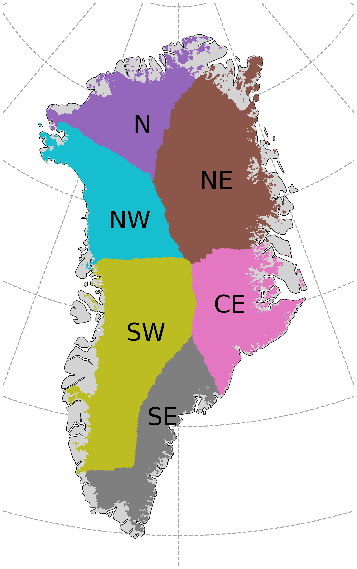
Figure 2Partitioning of Greenland into six basins N (north), NE (north-east), CE (central-east), SE (south-east), SW (south-west), NW (north-west) used in the evaluation.
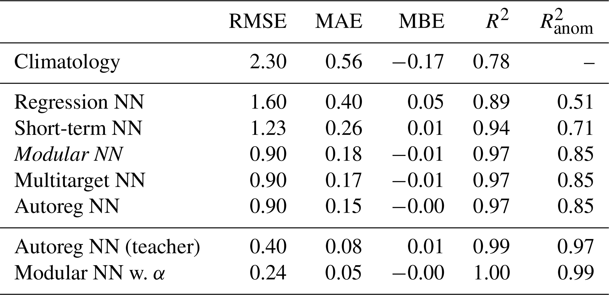
Table 3Performance for surface melt prediction of final models from the configuration study evaluated on the test set. RMSE, MAE, and MBE in mm w.e. per day; R2 the standard coefficient of determination, and is relative to anomalies from climatology. The five models are ordered by increasing model complexity. Autoreg NN (teacher) and Modular NN w. albedo use firn model output as input variables and are only listed for comparison.
3.1 Evaluation of the configuration study
We start by analyzing overall mean performance over the entire ice sheet. The performance of the best models from the tuning process (Appendix C: Table C1; Fig. C1a) on the test set are summarized in Table 3. All five configurations outperform the climatology benchmark, and performance increases with model complexity from a MAE of 0.40 mm w.e. per day for Regression NN, to 0.26 mm w.e. per day for Short-term NN, 0.18 mm w.e. per day for Modular NN, 0.17 mm w.e. per day for Multitarget NN, and 0.15 mm w.e. per day for Autoreg NN. The other metrics show improvement from Regression NN to Short-term and Modular NN, but then plateau. Thus, information about the past few days and long-term history is essential. Autoreg NN shows that the autoregressive element does not significantly improve performance further in inference mode, where previous predictions are recursively used as input. In contrast, evaluating Autoreg NN in teacher-forced mode demonstrates that information contained in the previous day’s melt is indeed predictive. This discrepancy indicates that, while the autoregressive signal is informative, its benefit is limited in practice by error propagation during recursive rollout.
The additional experiment using the Modular NN with α highlights the impact of albedo on accurately estimating surface melt, as providing α enables the model to achieve excellent performance with almost perfect R2 scores of 0.99. However, since albedo is an output of the firn model, this model configuration cannot be used as an emulator. Moreover, since albedo is strongly connected with surface temperature (given sufficient snow depth), it implicitly encodes the presence of melt, though it does not uniquely determine its magnitude. As a result, it remains unclear whether the improvement in melt prediction arises from the model accurately capturing absorbed shortwave radiation or simply from albedo serving as a direct indicator of melt on non–bare ice grid cells. In contrast, augmenting the model to predict albedo as an additional target (Multitarget NN) does not improve melt estimates.
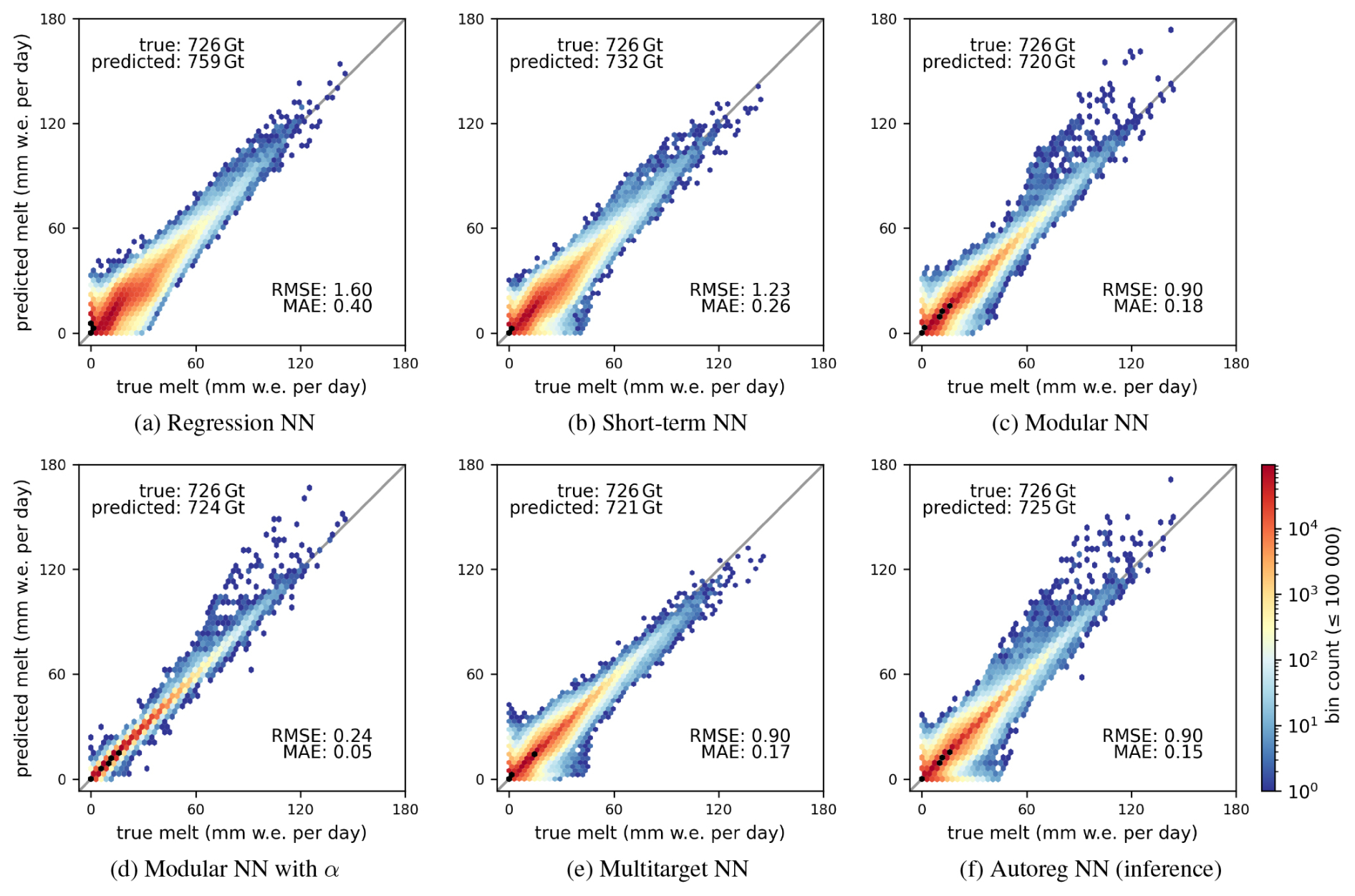
Figure 32D hexagonal binning plots of true versus predicted surface melt of the test set of the different models. Note that (d) uses the firn model output albedo as input variable and is thus only listed for comparison. The logarithmic color bar is valid for bins containing up to 105 data points; bins containing more than 105 points are indicated in black for better visibility.
3.1.1 Point-wise evaluation
Across all models, the RMSE substantially exceeds MAE, indicating considerable under- and overestimation of melt across melt events of all magnitudes, as shown by the dark blue colored hexagonal bins in Fig. 3. The superior performance of Modular NN, Autoreg NN, and Multitarget NN compared to Regression NN and Short-term NN stems primarily from improved predictions for a majority of data points for melt events up to 50 mm w.e. per day (narrower dark red band in Fig. 3c, e, f compared to a and b). For Modular NN, 64 % of the RMSE is attributable to absolute residuals up to 5 mm w.e. per day, a further 34 % to absolute residuals between 5 and 15 mm w.e. per day, and only 2 % of the RMSE to absolute residuals exceeding 15 mm w.e. per day.
Modular NN (Fig. 3c), Modular NN with α (Fig. 3d), and Autoreg NN (Fig. 3f) show some notable overestimation pattern of melt events above 50 mm w.e. per day. This systematic deviation originates from an unusually early melt event in April in the SW basin, where severe overestimation occurs on only one single day (Fig. D1). While the model successfully predicts the unusually early surface melt for most days during this event, one particular day exhibits sensible heat flux values up to 460 W m−2. While such extreme sensible heat flux values also appear in the training set, the combination of an anomalously large heat flux with unusually early melt creates conditions that are effectively out-of-sample.
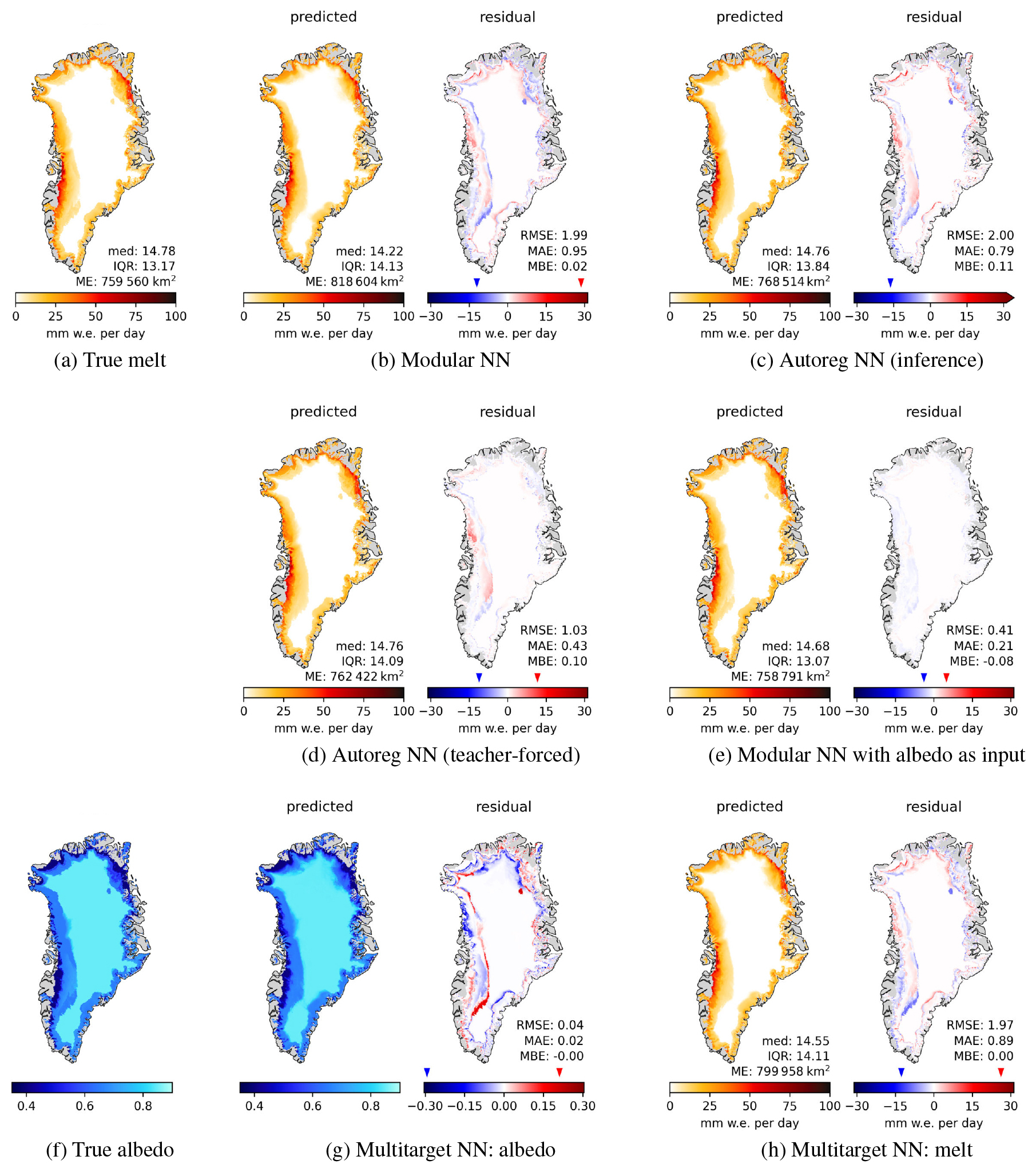
Figure 4Surface melt for 21 July 2016 with melt extent (ME) in km2, median and IQR of melt in mm w.e. per day. (a) true melt, (b) and (c) predicted melt (left panels) and residuals (right panels) of Modular NN and Autoreg NN (in inference mode). (d) and (e) show the predictions and residuals of Autoreg NN in teacher-forced mode, and of Modular NN with albedo as additional input; both these models cannot be used to produce predictions from climate forcing only, as they use firn model outputs as inputs. (f) shows the true albedo, (g) the albedo prediction and its residual, and (h) the melt prediction and its residual of Multitarget NN.
3.1.2 Qualitative assessment
But what causes these over- and underestimations? For this, we look at a typical day from the peak melt season in the test set in more detail. Figure 4 shows true and predicted melt, alongside residuals, for different models for a day in July. The melt maps are given together with the daily melt extent (ME) in km2, whereby we only consider melt > 1 mm w.e. per day, and its median and IQR in mm w.e. per day.
Modular NN predicts spatially over-smoothed melt fields, evident in both the predicted field itself and the residual map in Fig. 4b, which also leads to a larger ME. Autoreg NN in teacher-forced mode (Fig. 4d) shows substantial improvement in the spatial structure, with more pronounced contours in the predictions. However, the true previous melt used to make teacher-forced predictions is not available when applying the emulator to new climate data, where the model is run in inference mode, using its own prediction of the previous day. While the predicted melt field in inference mode (Fig. 4c) still exhibits sharper contours compared to Modular NN, the residual plot shows that there is uncertainty on where exactly these sharp contours should be.
Modular NN with α as an additional input shows that knowledge of surface albedo improves the spatial patterns significantly (Fig. 4e). This suggests that the autoregressive element's importance lies mainly in its role as a proxy for surface albedo, which in turn is also an indicator of melt presence. However, as noted above, this configuration cannot be used for predictive applications. The alternative model Multitarget NN, which uses albedo as an auxiliary target instead does not lead to noteworthy improvement of melt predictions (Fig. 4h). Unfortunately, the predicted albedo fields are also over-smoothed (Fig. 4f, g), with the residual map closely mirroring the spatial patterns of the melt residuals (Fig. 4h).
Daily maps for additional days throughout the year are shown in Appendix E, with the maps for a day in June (Fig. E3) and August (Fig. E4) showing similar spatial structures as those for July in Fig. 4. These results reveal the fundamental challenge: the simultaneous over- and underestimations arise from the model's inability to accurately reconstruct the sharp spatial structures of the surface state, which are present at the daily scale. Without explicit knowledge of surface albedo, the model produces smoothed fields that systematically overestimate melt in some locations while at the same time underestimating it in others, creating the characteristic spatial error pattern observed in the residuals.
3.2 Evaluation of the systematic input selection study
Since Modular NN, Autoreg NN, and Multitarget NN show very similar performance on the test set, we perform the systematic input selection study based on Modular NN as it is the least complex model among these three. Table 4 lists the performance of the Modular NN using different input subsets defined in Table 2 and Sect. 2.2.4. The metrics are given for the respectively best model from the tuning process (Appendix C: Table C2; Fig. C1b) on the test set.
Modular NN EBMTd does not show any significant improvement on the test scores compared to Modular NN with the default input set. However, Fig. 5 shows a better correspondence between true and predicted melt for the sparse high melt values compared to Modular NN (Fig. 3c). Especially the previously discussed melt overestimation due to the unusually high sensible heat flux (Fig. D1) does not happen anymore when using the energy inputs summed up, proving the stabilizing effect of using the energy terms summed up instead of separately.
Modular NN EBMT shows that including all atmospheric variables not just in the short-term module but their 10 year averages also in the long-term module improves model performance from RMSE of to , compared to using only snowfall and temperature as long-term conditions proxies. Removing T from the inputs (Modular NN EBM) improves performance on the test set only slightly. Having rainfall as inputs improves model performance slightly, since the metrics worsened for Modular NN EBS. Snowfall on the other hand is a very critical input, as RMSE increases by if the model is trained without snowfall (Modular NN EBR). While the relation between true and predicted values for all subsets look very similar, Modular NN EBR shows increased amount of small deviations up to 50 mm w.e. per day (wider spread of red band in Fig. F1e compared to a–d, f).
Thus, best model is achieved with EB terms (with LW↓, LHF, and SHF summed up, and SW↓ separate) and mass terms (especially snowfall) on a daily resolution for the current and the past 9 d, and additionally as 10 year averages. Furthermore, seasonal encoding is critical. Including air temperature T, which often serves as melt proxy, cannot improve model performance any further. In contrast, including T increases model size by 11 additional input features, and it can impair model interpretability since T is not a causal input to melt production, but a confounding variable for turbulent heat fluxes and melt. Moreover, while T does impact the test scores only slightly, the generalizability to future climate projections could be affected by including T as an input variable. Melt models based on T as proxies often under- or overestimate melt under a warming climate, as they do not consistently include melt-albedo feedback, changed cloud formation and thus change in radiative inputs (Goelzer et al., 2013; Bolibar et al., 2022). While the applicability of ML models to future projections must always be evaluated separately, air temperature could rather be a confounding variable decreasing model performance and transferability to different climates, than being a useful predictor.
Table 4Performance of final models on the test set for the default Modular NN and its variations using different input variable subsets consisting of energy balance terms (EB), mass terms M (rainfall (R) and snowfall (S)), temperature T, and seasonality encoding (with noDOY indicating seasonality encoding was removed as input). RMSE, MAE, and MBE in mm w.e. per day; R2 the standard coefficient of determination, and is relative to anomalies from climatology.
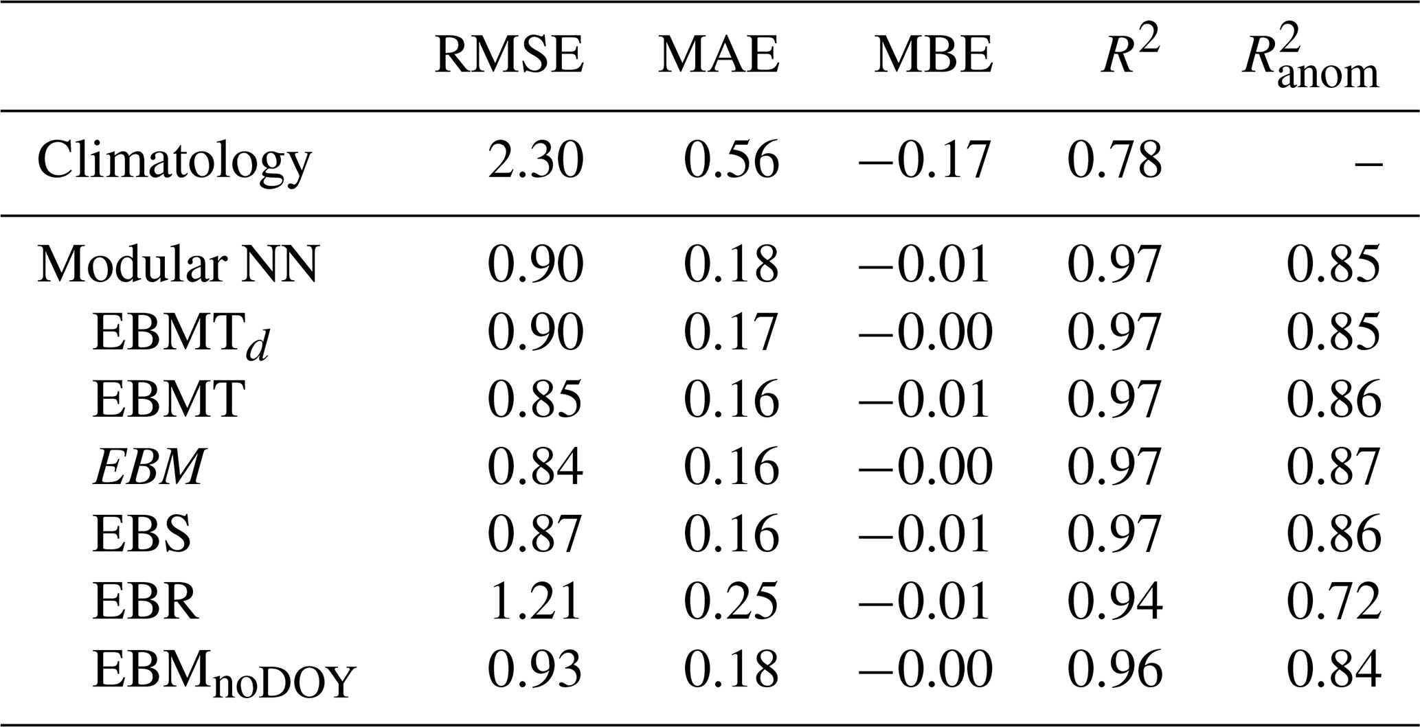
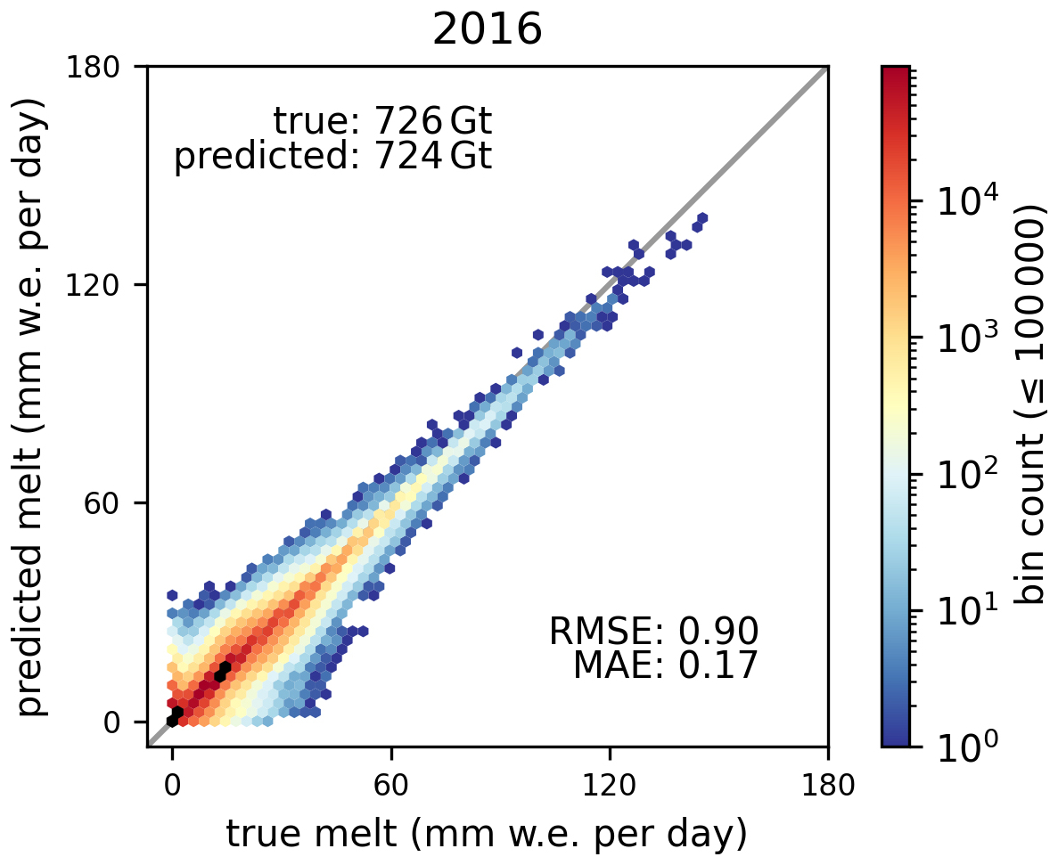
Figure 52D hexagonal binning plots of true versus predicted surface melt of the test set of Modular NN EBMTd. The logarithmic color bar is valid for bins containing up to 105 data points; bins containing more than 105 points are indicated in black for better visibility.
3.2.1 Spatial-temporal residual distribution
In the remainder of this section we investigate the performance of Modular NN EBM spatially and temporally. This analysis includes predictions from both the test year 2016 to show the error patterns of a single independent year and the entire period 1990–2016 to investigate persistent systematic biases of our model.
Figure 6 shows the seasonally aggregated melt for the test set, starting from December 2015 to November 2016. The overestimated melt extent and lower median of melt predictions compared to true melt in the daily maps for Modular NN (Fig. 4, Appendix E) is also visible in the seasonal aggregates of Modular NN EBM across all seasons. The south-west coast shows some underestimation in surface melt in spring (MAM, Fig. 6b), which intensifies in summer (JJA, Fig. 6c). In contrast the north and north-west coastal region shows overestimation in summer. However, Fig. 7 shows that this melt overestimation in JJA is a behavior more specific to the test year, rather than a characteristic of the model Modular NN EBM. The residual plot for JJA averaged across 1990–2016 shows systematic underestimation of melt within the whole ablation zone, and some overestimation at the transition between ablation and percolation zone especially in the north and north-west (compare GrIS zones Fig. B1). Together with the superior performance of Modular NN with α this indicated that the underestimation stems from the lowered albedo for shallow snow depths and bare ice. The long-term variables using 10 year averages in combination with the daily variables for in total 10 days are not enough to derive snow depth and thus decreased albedo due to bare ice exposure. Including variables at a monthly or quarterly scale leading up to the prediction day might help in approximating snow depth and associated albedo.
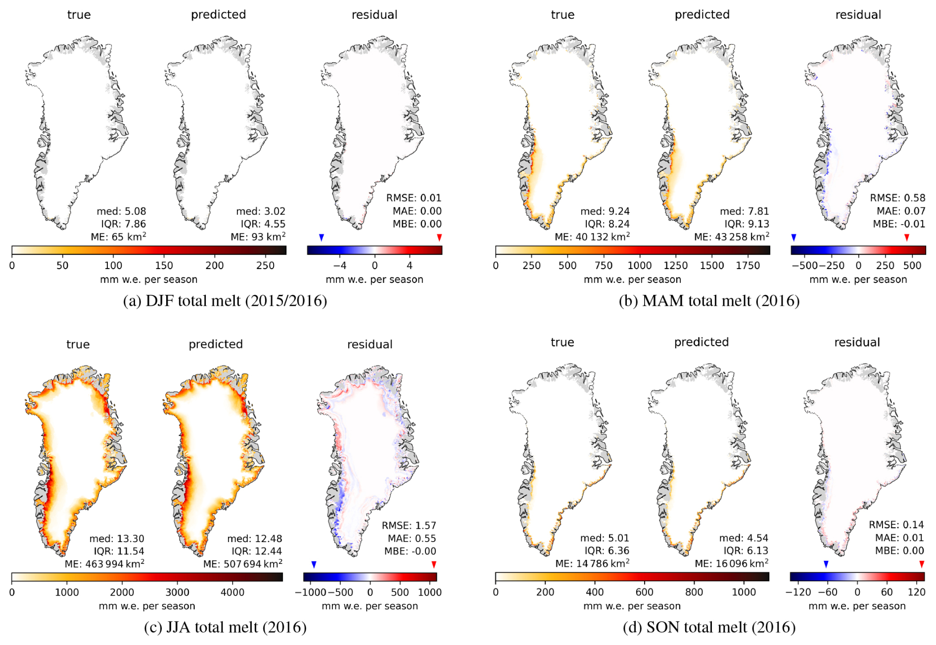
Figure 6True melt alongside melt predictions and residuals of Modular EBM seasonally aggregated for the test set, but with December in (a) taken from 2015. (a) December, January, February; (b) March, April, May; (c) June, July, August; (d) September, October, November. Note that color scales are adjusted individually for each subplot.
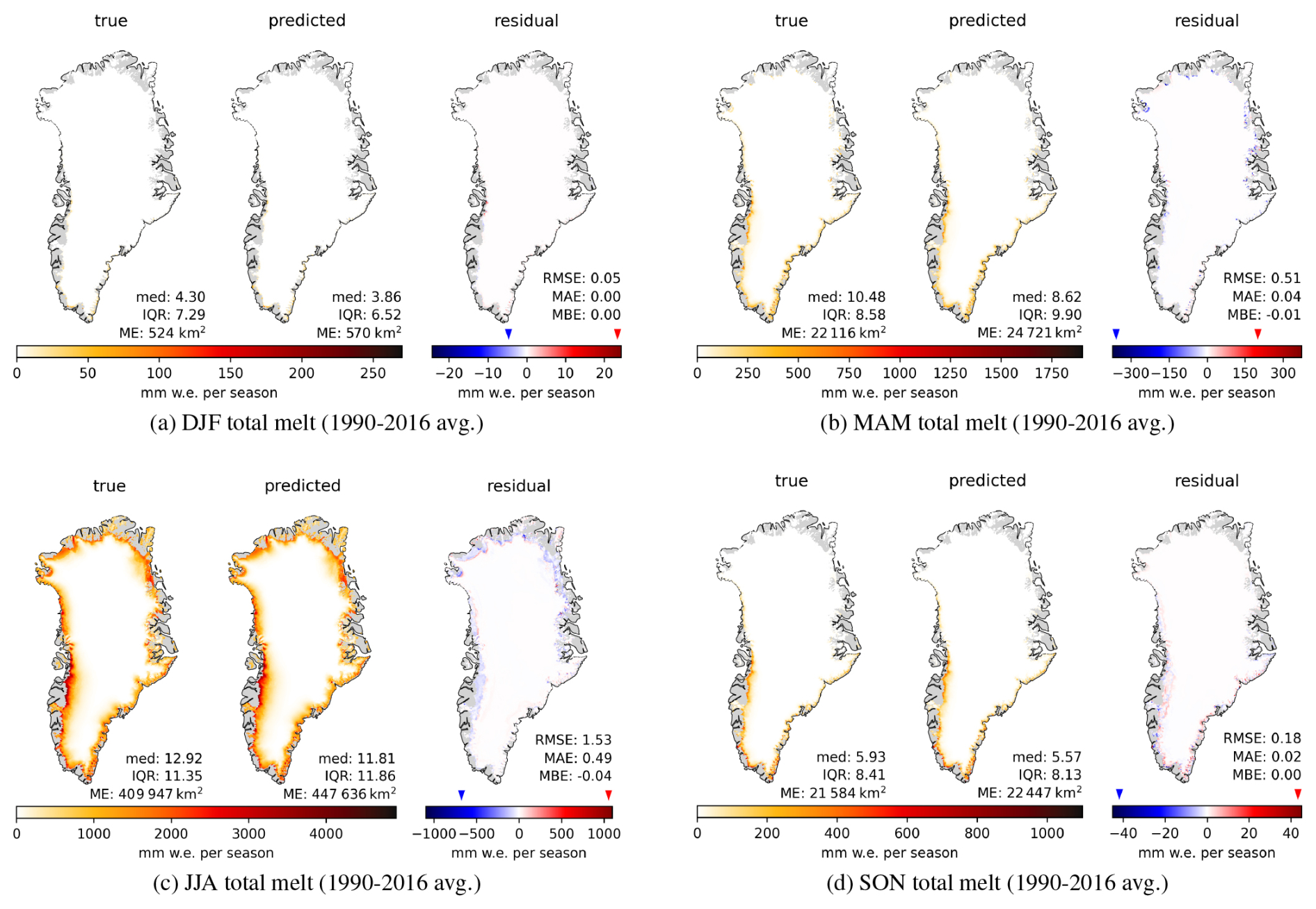
Figure 7True melt alongside melt predictions and residuals of Modular EBM seasonally aggregated per year, and averaged across 1990–2016. Note that color scales are adjusted individually for each subplot.
In the remainder of this section we investigate the performance of Modular NN EBM at the basin level. To enable performance comparison across the six basins, we present the mean annual melt and performance scores for each basin and the whole ice sheet in Table 5. The melt amount and the scores are given for the test year 2016, together with the mean ± standard deviation of the single years for the entire period 1990–2016. Figure 8 shows basin-wise integrated true and predicted melt for the test year alongside their climatologies, together with daily over- and estimation throughout the annual cycle for the test year (middle rows) and averaged over all years 1990–2016 (bottom rows).
Basins SE and SW show the highest melt with respect to their basin area, and also the highest year-to-year fluctuations in melt amount, followed by basin N (Table 5). Correlation R2 between true and predicted melt is high across all basins, with the northern basin having slightly lower R2 (0.95–0.97) than the southern basins (0.98). The computed on anomalies from the climatology is highest for the southern basins SE and SW (0.93 and 0.92), with low standard deviation of 0.02. In contrast, the northern basins N and NE show of 0.78 and 0.75 respectively, paired with higher standard deviations of 0.07 and 0.11 respectively. This indicates that the emulator captures variability with respect to the climatology particularly well in the SW and SE basins, which have stronger anomalies that the model can learn, while the other basins show lower anomaly skill.
In accordance with that, the RMSE mean and standard deviations are highest for basins N and NE compared to the other basins. Also, as with the whole ice sheet, MAE is significantly lower than RMSE for all basins, indicating that a few large residuals persist across all regions. The MAE-to-RMSE ratio indicates that basins NE and NW are affected most by a small number of high residuals, while basins SW and SE are the least dominated by such outliers, and more by small and medium errors.
Basin SE is the only one with a positive bias on average (0.01), while the other basins show zero or slightly negative MBE of −0.02 at most on average across the years. However, the respective standard deviations across the years are bigger than the absolute means of the biases, i.e. no basin has a systematic bias across the years. Basins N and SW show the largest fluctuations in bias with a standard deviation of 0.05, while they also show high average melt together with high melt variability relative to mean melt amount (27 %), and thus these basins are particularly variable and hard to learn.
Figure 8 shows that not only is there no systematic bias across the years, but also that over- and underestimating melt is largely synchronous, thus there are also no pronounced systematic temporal biases. However, basins N and NW show a tendency toward early-season underestimation and late-season overestimation, while basin NE shows a dominance of underestimation throughout the entire year.
2016 is a relatively high melt year for each basin, but within one standard deviation from the respective means. Basins N and NW show anomalous positive MBE of 0.06 and 0.05 respectively, while basin SW shows strong negative bias of −0.06, such that the biases cancel each other out across the whole GrIS. Figure 8 shows enhanced melt at peak melt season for basins N and NE, causing more melt overestimation than normal, and higher . Basin NW also shows high melt at peak season, but then a sudden decrease end of July, and thus the melt amount deviates significantly from the climatology which leads to a 1.5 standard deviation lower than for the average year. Also SW and to a lesser extent CE and SE have lower than the average year as they show a lot of temporal fluctuation in the melt (top panels in Fig. 8 SW and SE), also starting with some early melt. For SW and SE the RMSE and MAE are also more than a standard deviation above the average.
These deviations in 2016 highlight the model's challenges in capturing anomalous melt patterns that deviate substantially from the climatological mean, particularly in basins with pronounced seasonal deviations such as NW's abrupt late-summer decline and early melt onset in basins SW and SE. However, while individual basin biases in 2016 are notable (positive for N and NW, negative for SW), these deviations appear to be year-specific rather than systematic. Averaging across the entire 1990–2016 period reveals that the model exhibits no persistent systematic biases, with year-to-year fluctuations in error patterns largely balanced over time. Although based on the performance including the training set, this temporal stability suggests that the emulator's performance is robust across the multi-decadal timescale.
Table 5Performance of Modular NN EBM for predicting surface melt per basin and over the entire GrIS for the test year 2016, together with mean ± standard deviation across the full period 1990–2016. Spatial mean annual melt, RMSE, MAE, and MBE in mm w.e. per day.
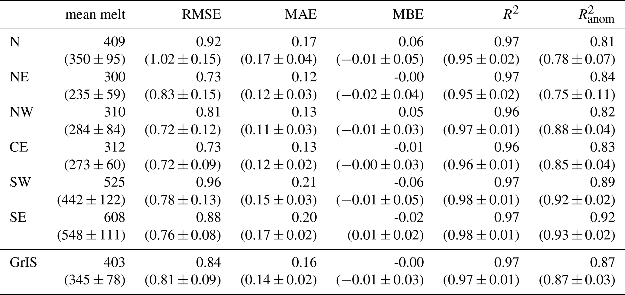
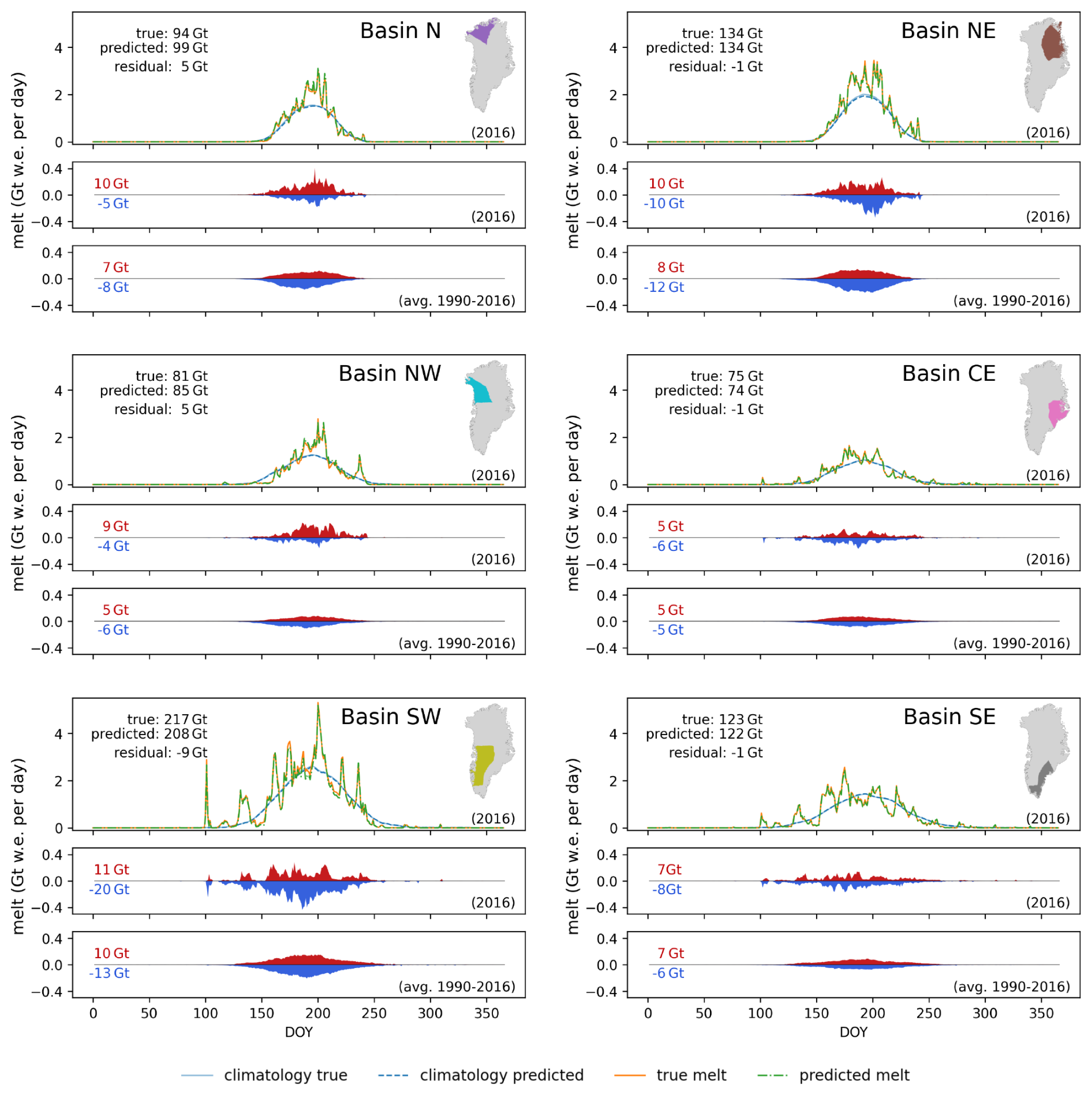
Figure 8Temporal distribution of over- and underestimations of Modular NN EBM per basin. The respective upper subplots show the basin-wise total true and predicted surface melt for the test year together with the true and predicted melt climatologies (1990–2013). The middle subplots show the total amount of overestimated (red) and underestimated (blue) melt per basins for the test year. The lower subplots show the average annual overestimated and underestimated melt for the whole time period 1990–2016.
We have developed a machine learning emulator that successfully predicts daily surface melt on the Greenland ice sheet from atmospheric variables alone. By training a neural network on 24 years of output from the polar regional climate model HIRHAM5 and its firn model DMIHH, we demonstrate that surface melt can be accurately emulated with a mean absolute error of 0.16 mm w.e. per day (Table 4), significantly outperforming climatological benchmarks. Basin-level evaluation demonstrates that our location-agnostic approach generalizes well across the diverse climatic regimes of Greenland. The emulator maintains high correlation across all six major basins with minimal systematic bias (Table 5).
Our iterative model development reveals several key insights about the role of temporal information. Including atmospheric conditions from the previous nine days substantially improves performance over using only current-day conditions, demonstrating that short-term history matters. Furthermore, long-term climate memory in the form of decadal averages of temperature and snowfall improve model performance by providing crucial information about location-specific firn characteristics that affect the surface energy balance. Thus, the model profits from short- and long-term memory from these past conditions. Beyond the climate forcings that directly impact SEB, i.e., turbulent heat fluxes and radiation, also snowfall and seasonality encoding are crucial input parameters. Rainfall does improve model performance but only slightly, while air temperature does not contribute to any additional performance increase, and should therefore be excluded from emulation approaches particularly when the model is combined with explainability algorithms, where redundant variables can obscure interpretability (Molnar et al., 2022; Jiang et al., 2024).
The predicted melt fields tend to be spatially over-smoothed compared to the firn model output, lacking sharp transitions between regions of different melt extent which are a consequence of the albedo scheme using lower albedo for bare ice and small snow depths. Neither an autoregressive approach (Autoreg NN) nor learning albedo as an auxiliary target (Multitarget NN) did improve this over-smoothing. Therefore, capturing the sharp spatial gradients emerging from different surface conditions remains a fundamental challenge for data-driven approaches using atmospheric input data only. Future work should explore whether incorporating more versatile historical information, such as accumulation and energy input from preceding months, can help differentiate high versus low snow regimes. The neural network architecture could be extended with a module operating on monthly timescales, or more sophisticated approaches for timeseries modeling, such as LSTMs (Hochreiter and Schmidhuber, 1997) or transformer-based architectures (Vaswani et al., 2017), could be investigated.
Additionally, the domain of applicability must be determined and extended. The emulator is developed on HIRHAM5 reanalysis data and trained to emulate DMIHH firn model behavior. Extrapolation beyond the training distribution yields unreliable results in data-driven approaches, and it is unclear to what extent different simulations deviate in their data distribution and how sensitive the emulator is to these changes. Applying the emulator to climate data under different forcings, from different time periods, or from entirely different polar RCMs thus likely requires retraining. Furthermore, in the future the emulator can be extended to predict additional firn model outputs, such as runoff, creating a more comprehensive tool for Greenland SMB estimation.
In conclusion, this work demonstrates that machine learning can successfully emulate firn model behavior with spatially and temporally consistent accuracy and computational efficiency, while also revealing fundamental challenges in capturing sharp spatial patterns driven by surface characteristics. This emulator, when coupled with downscaling emulators that bridge the gap between global climate models and regional applications, enables the large ensemble projections needed to quantify uncertainty both within individual RCMs and across the divergent projections from different polar RCMs. Furthermore, such a firn emulator can be used as a surrogate model for SMB processes in Earth system models, enabling interactive ice sheet-climate coupling at scales previously computationally infeasible.
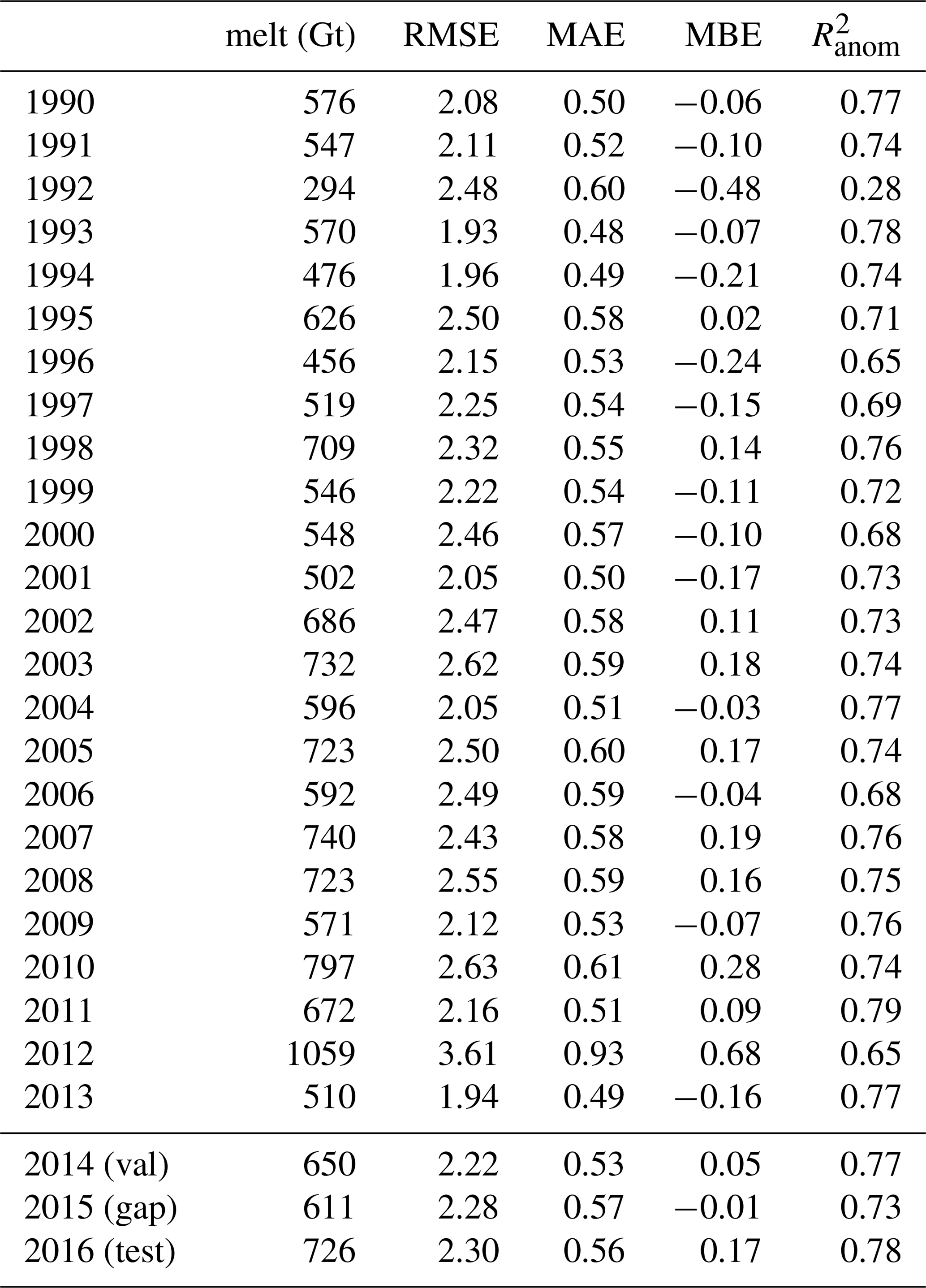
Table A1 shows aggregated melt characteristics per year compared to the climatology over 1990-2013. The total melt of the validation year (650 Gt) and the test year (726 Gt) lie well within the historical range of the training climatology (294-1059 Gt) and are comparable to several years in the record (e.g., 1995, 2002, 2011, and 1998, 2003, 2005, 2007, 2008 respectively), deviating from the climatological mean by less than 0.75 standard deviations. The MBE exhibits a clear shift from predominantly negative values (until 2002) to positive values thereafter. Despite this overall change, the deviation metrics w.r.t. the climatological melt for 2014 and 2016 align well with other years in the dataset, suggesting these are climatologically typical years rather than anomalous ones. This assessment is supported by the Arctic reports Jeffries et al. (2014); Richter-Menge et al. (2016), which document that 2014 and 2016 reflect the increasing melting trend without reaching the extremes of previous record years.
Table A1Total melt (in Gt per year); RMSE, MAE and MBE (in mm w.e. per day) relative to the climatology over 1990–2013, and the coefficient of determination between the specific year and the climatology ().
The spatial sub-sampling of 5000 grid-cells is performed according to predefined zone specific probabilities. The probabilities are chosen to be of 65 % for the ablation zone, 30 % for the percolation zone, and 5 % for the dry-snow zone. Here, the zones are defined based on the SMB from the 10 year time range 1990–1999, with the ablation zone having negative SMB, the dry-snow zone showing melt below 100 mm w.e. per year for each year, and the percolation zone covering the remaining grid cells of positive SMB but non-negligible melt (Fig. B1). Alternative sampling strategies were not formally evaluated, as the chosen approach was sufficient for the modeling objectives and computational constraints of this study. Model results indicate that the main source of predictive error is related to unknown surface conditions, especially albedo, rather than the quantity of training data. This suggests that increasing the amount of training data would not necessarily reduce prediction errors, and that effective model training could potentially be achieved with fewer data points.
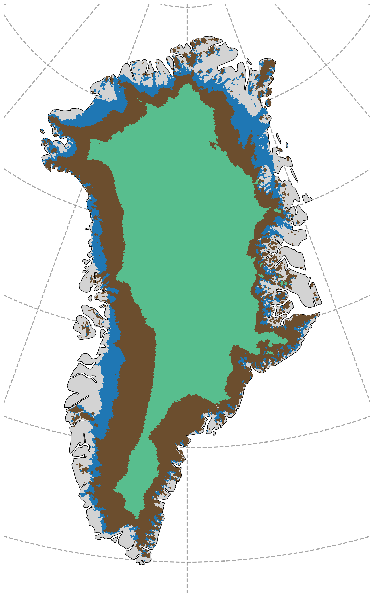
Figure B1Ablation (blue), percolation (brown), and dry-snow (green) zone used for spatial sub-sampling.
Hyperparameters in ML algorithms are settings that control the algorithm’s behavior, but are not adapted by the learning algorithm itself. This includes the choices of the architecture itself, its capacity, the activation function, regularization techniques, initialization, optimization algorithms and their specific setting, and more. Since it is unfeasible to tune all these hyperparameters, well-informed choices must be made to prioritize the most impactful parameters. The Modular NN architecture was defined based on physical principles, and we explore different architectural configurations to identify the most suitable design. The network capacity (number of layers and neurons per layer) was chosen to be sufficiently large, as evidenced by overfitting observed during training. To prevent using an overfitted model, we select the model weights that yield the lowest validation loss, which effectively corresponds to regularization via early stopping. The batch size is fixed at the maximum value permitted by available computing resources. Given these design choices, we primarily focus on tuning the learning rate for each configuration, as it is the most critical factor for training convergence and optimization performance (Goodfellow et al., 2016).
Table C1 presents the overview of the NN configurations, the tuned hyperparameter ranges, alongside RMSE, MAE, and MBE of the validation set of the best performing model for each configuration across all tuning trials. We define the best performing model by the sum of the relative MAE and MBE w.r.t. the seasonal anomaly errors. Fig. C1a shows the performance of all the trials, with the more complex models having consistently better performance than the less complex models. The results of Multitarget NN are not plotted, since they strongly coincide with the performance of Modular NN.
For each of the five configurations, we tuned the learning rate. For Modular NN, we additionally tuned the number N of preceding days used as input, to determine the optimal number of input days, which was then fixed when tuning the subsequent configurations. As Multitarget NN has a composite loss function consisting of both melt and albedo terms, the weighting between those two components is crucial. Therefore, while tuning the learning rate we simultaneously varied the weighting factors of melt MSE and albedo MSE for calculating the total loss, testing the following melt:albedo weight–ratios: 1:1, 7:3, 9:1, and 3:7. Further, we took a second attempt using trainable weights as proposed in Cipolla et al. (2018).
We trained the configurations one after another, using insights from each result to guide the development of the next configuration. While performance generally improves with more preceding days, gains become marginal beyond 8 d, with 9 d achieving the best score. Therefore, the subsequently trained configurations Short-term NN, Autoreg NN, and Multitarget NN use 10 input days (i.e., N=9 preceding days), with the learning rate being tuned for 33 trials. We also narrowed the range of possible learning rate values when progressing through the different configurations as we gained insight into which ranges make sense.
When training the autoregressive NN under teacher-forced mode, we use the true melt with random noise, i.e., SM with to get more robustness and not rely too much on the previous melt input. The results of Autoreg NN (teacher) show that the model benefits significantly from knowing the previous day's surface melt. However, this advantage diminishes when the model is evaluated in inference mode, i.e., when using the previous prediction instead of the true melt. We alternatively tested different strategies of training autoregressively with using the previous predicted melt during training, using different ratios of teacher-forced versus true melt, and different lengths of rollout windows. Although RMSE slightly improved, MAE and MBE did not decrease, and the same error patterns observed for the modular NN (which are discussed in the qualitative assessment in Sect. 3.1.2) remained. Furthermore, the autoregressive training requires much higher computing resources, since a prediction for a specific day requires to make the prediction for the previous day(s), which also required a decreased batch size during training.
As baseline for information gain from the variable albedo, we retrain Modular NN including albedo in the set of daily input variables. This leads to a RMSE of 0.22, MAE of 0.05, and MBE of mm w.e. per day on the validation set.
Modular NN is then trained using different variable subsets as inputs as defined in Table 2. Each of the variations have been trained 33 times with optimizing the learning rate within the range . For each subset, the performance scores of the best performing model across all trials (in terms of the sum of the relative MAE and MBE w.r.t. the seasonal anomaly) are listed in Table C2. Figure C1b shows the performance of all the trials.
Table C1Network Tuning: Overview of the five network configurations with the tuning parameter ranges, and their validation scores in mm w.e. per day. The performance of Autoreg NN is stated in teacher-forced and in inference mode.
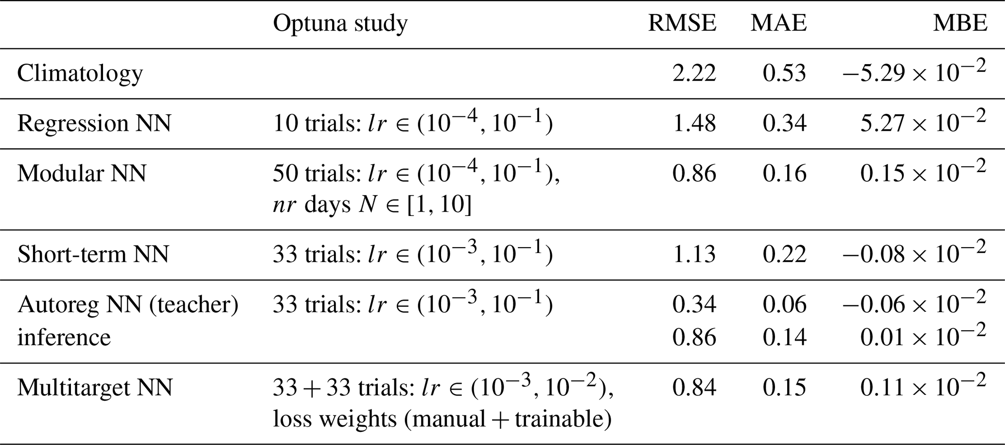
Table C2Input selection study: Overview of Modular NN using different input variable subsets, with the validation scores in mm w.e. per day.
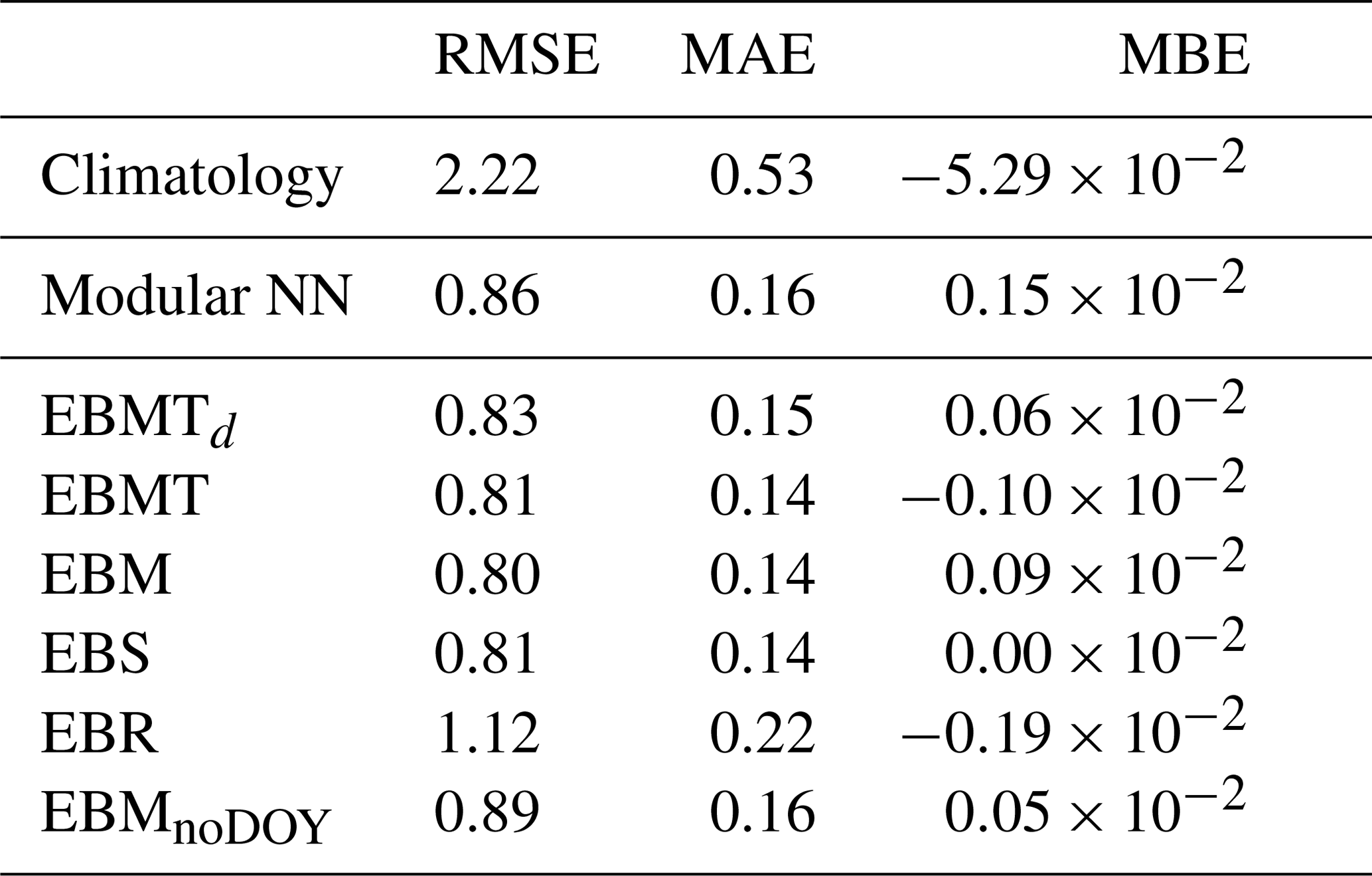
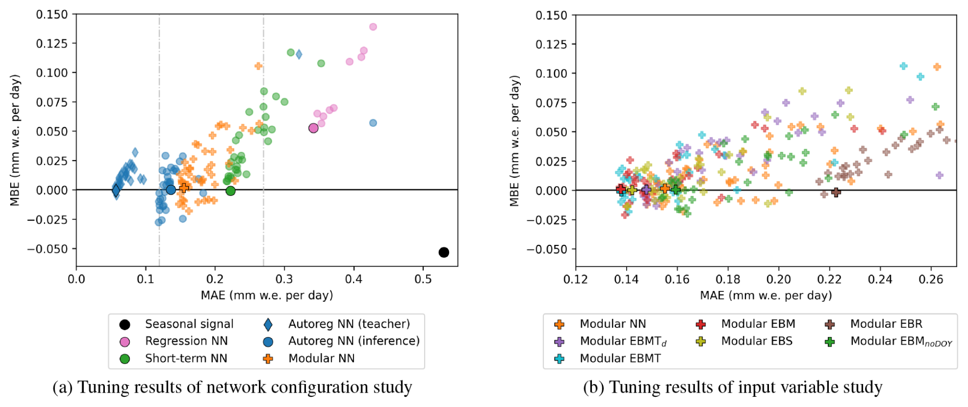
Figure C1MAE and MBE on the validation set of the tuned models. The best performing model for each configuration is indicated by the black outlined shapes. (a) Models from the network configuration study: The seasonal signal (black circle) is the melt climatology over the years 1990–2013, smoothed with a 15 days window. The tuned networks Regression NN, Modular NN, Short-term NN, and Autoreg NN (in inference mode) are indicated by circles; Autreg NN in teacher-forced mode cannot be interpreted as applicable model, since it relies on the true melt and can only be used in its inference state, and is indicated with diamond symbol. Modular NN is indicated with the “plus” symbols, and shows the results for the input ablation study. The vertical gray dotted lines indicate the MAE range in panel (b). (b) Models from the input selection study: The Modular NN from the network configuration study is again depicted in orange color.
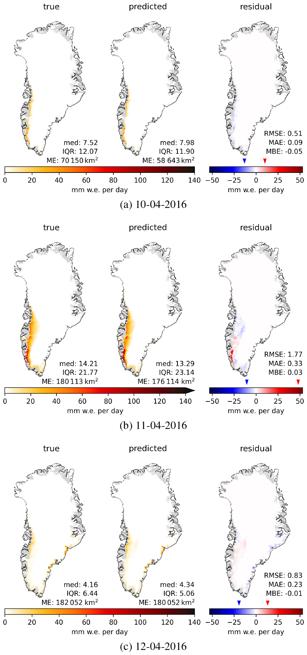
Figure D1True melt, and predicted melt by Modular NN with associated residual for three consecutive days in April 2016, with (b) causing the positive residual outliers shown in Fig. 3c. The blue and red triangles on the residual color bar indicate the highest negative and positive residual of that day, respectively.
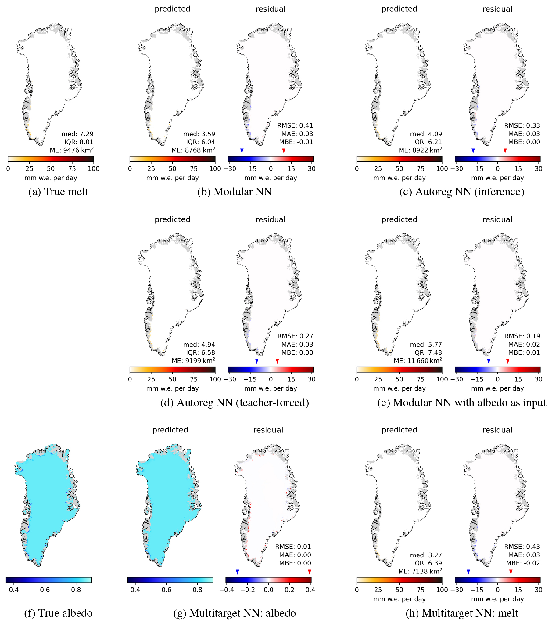
Figure E1Surface melt for 21 April 2016 with melt extent (ME) in km2, median and IQR of melt in mm w.e. per day. (a) True melt, (b)–(e), (h) predicted melt (left panels) and residuals (right panels); (f) true albedo and (g) predicted albedo and residual as additional outputs of Multitarget NN.
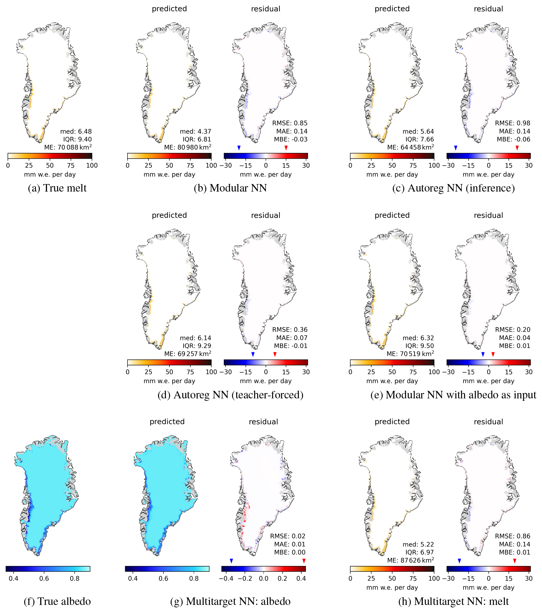
Figure E2Surface melt for 21 May 2016 with melt extent (ME) in km2, median and IQR of melt in mm w.e. per day. (a) True melt, (b)–(e), (h) predicted melt (left panels) and residuals (right panels); (f) true albedo and (g) predicted albedo and residual as additional outputs of Multitarget NN.
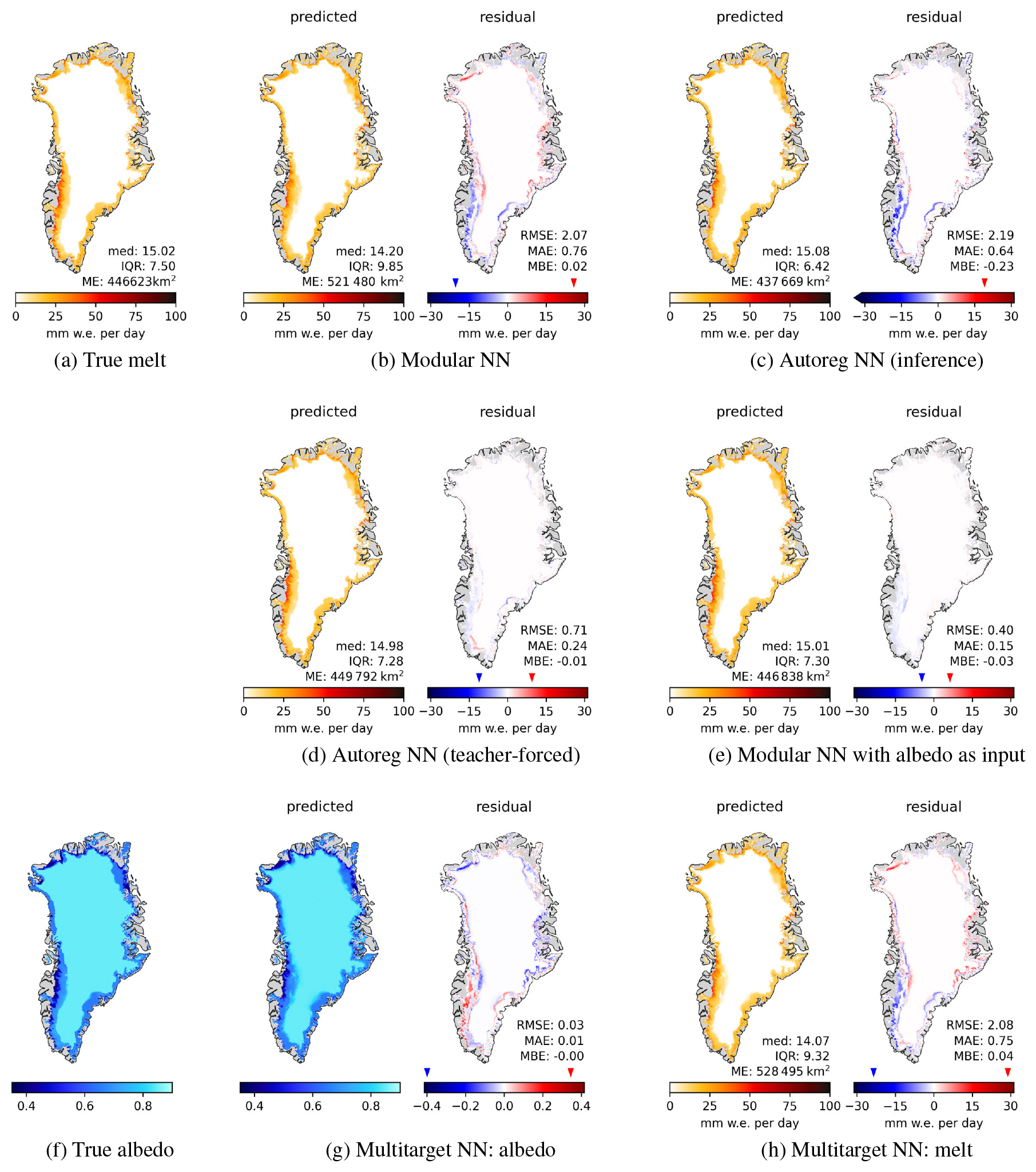
Figure E3Surface melt for 21 June 2016 with melt extent (ME) in km2, median and IQR of melt in mm w.e. per day. (a) True melt, (b)–(e), (h) predicted melt (left panels) and residuals (right panels); (f) true albedo and (g) predicted albedo and residual as additional outputs of Multitarget NN.
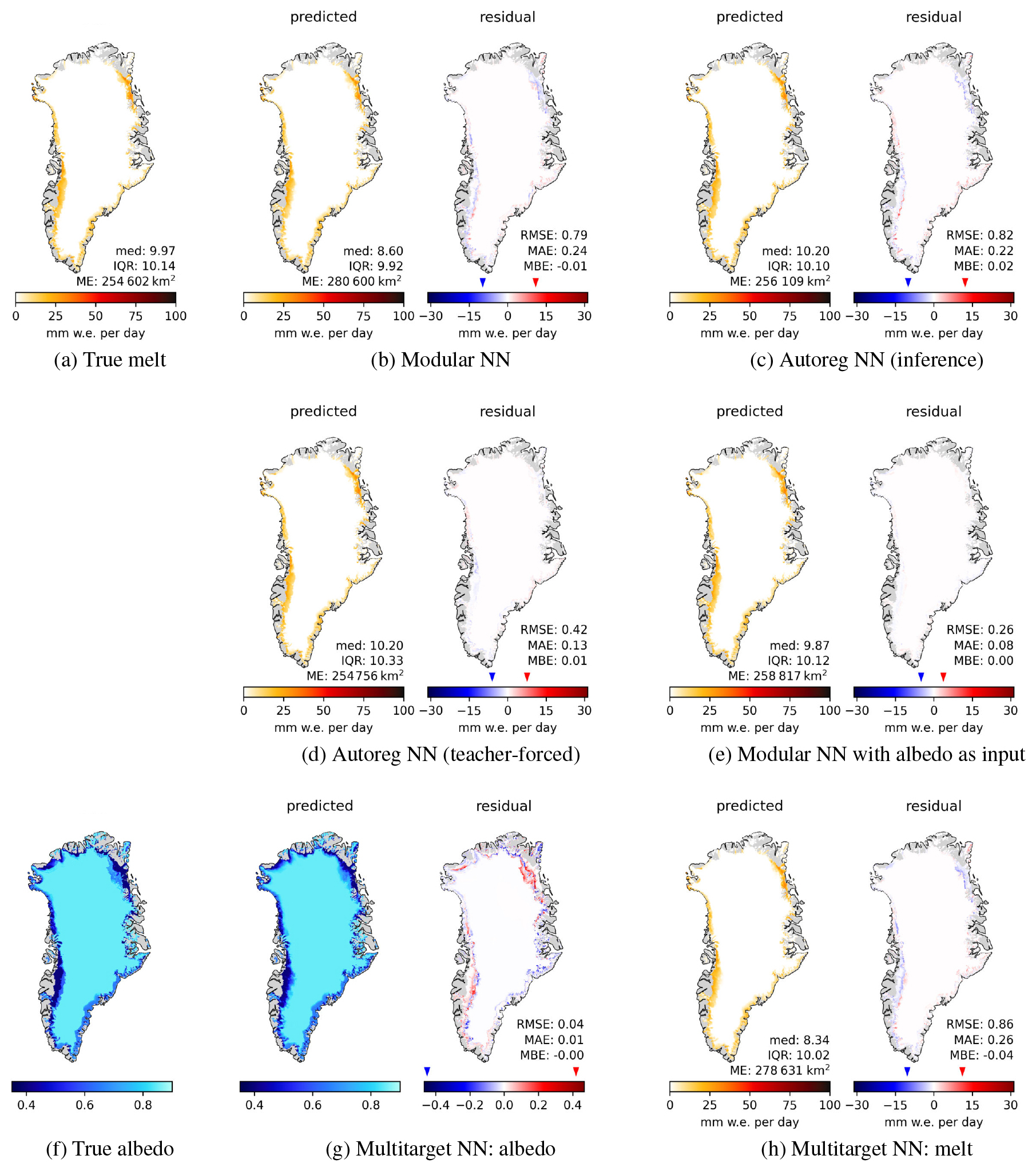
Figure E4Surface melt for 21 August 2016 with melt extent (ME) in km2, median and IQR of melt in mm w.e. per day. (a) True melt, (b)–(e), (h) predicted melt (left panels) and residuals (right panels); (f) true albedo and (g) predicted albedo and residual as additional outputs of Multitarget NN.
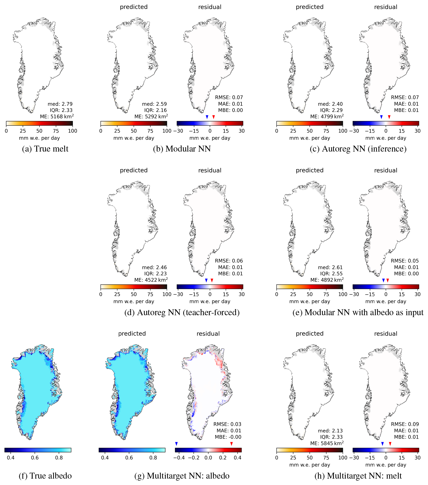
Figure E5Surface melt for 21 September 2016 with melt extent (ME) in km2, median and IQR of melt in mm w.e. per day. (a) True melt, (b)–(e), (h) predicted melt (left panels) and residuals (right panels); (f) true albedo and (g) predicted albedo and residual as additional outputs of Multitarget NN.
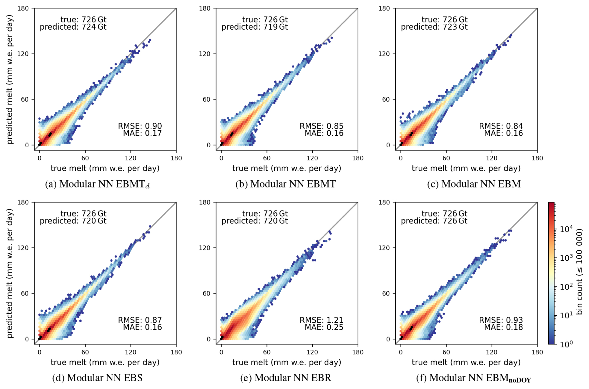
Figure F12D hexagonal binning plots of true versus predicted surface melt of the test set of Modular NN using different input subsets. The logarithmic color bar is valid for bins containing up to 105 data points; bins containing more than 105 points are indicated in black for better visibility.
Code is published under the MIT License and can be accessed via the GitHub repository https://github.com/eschlager/MeltEmulation/tree/revision (last access: 28 May 2026) or the Zenodo archive https://doi.org/10.5281/zenodo.20271069 (Schlager, 2026a). The data produced in this study is available at https://doi.org/10.5281/zenodo.19627367 (Schlager, 2026b). The HIRHAM5 simulation data is freely available upon request (Langen et al., 2017).
ES, PL, and RM conceptualized the study and designed the methodology. ES did the code implementation, computational experiments, and visualization. ES performed the analysis and validation with consultation from SS. ES prepared the original draft of the manuscript, with help from SS, PL, and RM. RM provided the financial support and access to computing resources.
At least one of the (co-)authors is a member of the editorial board of The Cryosphere. The peer-review process was guided by an independent editor, and the authors also have no other competing interests to declare.
Publisher's note: Copernicus Publications remains neutral with regard to jurisdictional claims made in the text, published maps, institutional affiliations, or any other geographical representation in this paper. The authors bear the ultimate responsibility for providing appropriate place names. Views expressed in the text are those of the authors and do not necessarily reflect the views of the publisher.
The original climate model simulations used in this project were carried out under the framework of the European Union's Horizon 2020 research project PROTECT under grant agreement 869304. We gratefully acknowledge the computing resources provided by the European Weather Cloud under special project dkmottr2. Claude Sonnet 4.5 was used for grammar check and to improve readability.
ES received support for this study from the National Centre for Climate Research (NCKF) and some additional support from the Novo Nordisk funded PRECISE project (grant no. NNF23OC0081251). SS received financial support from FWF project Weg_re (grant no. 10.55776/P35388).
This paper was edited by Andrew Orr and reviewed by two anonymous referees.
Akiba, T., Sano, S., Yanase, T., Ohta, T., and Koyama, M.: Optuna: A next-generation hyperparameter optimization framework, in: Proceedings of the 25th ACM SIGKDD international conference on knowledge discovery & data mining, 2623–2631, https://doi.org/10.1145/3292500.3330701, 2019. a
Anilkumar, R., Bharti, R., Chutia, D., and Aggarwal, S. P.: Modelling point mass balance for the glaciers of the Central European Alps using machine learning techniques, The Cryosphere, 17, 2811–2828, https://doi.org/10.5194/tc-17-2811-2023, 2023. a, b
Auffarth, B.: Machine learning for time-series with Python, Packt Publishing United Kingdom, ISBN: 9781801819626, 2021. a
Bolibar, J., Rabatel, A., Gouttevin, I., Galiez, C., Condom, T., and Sauquet, E.: Deep learning applied to glacier evolution modelling, The Cryosphere, 14, 565–584, https://doi.org/10.5194/tc-14-565-2020, 2020. a
Bolibar, J., Rabatel, A., Gouttevin, I., Zekollari, H., and Galiez, C.: Nonlinear sensitivity of glacier mass balance to future climate change unveiled by deep learning, Nat. Commun., 13, 409, https://doi.org/10.1038/s41467-022-28033-0, 2022. a
Chen, T. and Guestrin, C.: XGBoost: A Scalable Tree Boosting System, in: Proceedings of the 22nd ACM SIGKDD International Conference on Knowledge Discovery and Data Mining, KDD '16, 785–794, Association for Computing Machinery, New York, NY, USA, San Francisco, California, USA, ISBN 9781450342322, https://doi.org/10.1145/2939672.2939785, 2016. a
Cipolla, R., Gal, Y., and Kendall, A.: Multi-task Learning Using Uncertainty to Weigh Losses for Scene Geometry and Semantics, in: 2018 IEEE/CVF Conference on Computer Vision and Pattern Recognition, 7482–7491, ISBN 2575-7075, https://doi.org/10.1109/CVPR.2018.00781, 2018. a, b
de Burgh-Day, C. O. and Leeuwenburg, T.: Machine learning for numerical weather and climate modelling: a review, Geosci. Model Dev., 16, 6433–6477, https://doi.org/10.5194/gmd-16-6433-2023, 2023. a
de Roda Husman, S., Hu, Z., van Tiggelen, M., Dell, R., Bolibar, J., Lhermitte, S., Wouters, B., and Munneke, P. K.: Physically-informed super-resolution downscaling of Antarctic surface melt, Wiley Online Library, J. Adv. Model. Earth Syst., 16, e2023MS004212, https://doi.org/10.1029/2023MS004212, 2024. a, b
Dubey, S. R., Singh, S. K., and Chaudhuri, B. B.: Activation functions in deep learning: A comprehensive survey and benchmark, Neurocomputing, 503, 92–108, https://doi.org/10.1016/j.neucom.2022.06.111, 2022. a
Dunmire, D., Wever, N., Banwell, A. F., and Lenaerts, J. T. M.: Antarctic-wide ice-shelf firn emulation reveals robust future firn air depletion signal for the Antarctic Peninsula, Commun. Earth Environ., 5, 100, https://doi.org/10.1038/s43247-024-01255-4, 2024. a
Fettweis, X., Franco, B., Tedesco, M., van Angelen, J. H., Lenaerts, J. T. M., van den Broeke, M. R., and Gallée, H.: Estimating the Greenland ice sheet surface mass balance contribution to future sea level rise using the regional atmospheric climate model MAR, The Cryosphere, 7, 469–489, https://doi.org/10.5194/tc-7-469-2013, 2013. a
Fettweis, X., Box, J. E., Agosta, C., Amory, C., Kittel, C., Lang, C., van As, D., Machguth, H., and Gallée, H.: Reconstructions of the 1900–2015 Greenland ice sheet surface mass balance using the regional climate MAR model, The Cryosphere, 11, 1015–1033, https://doi.org/10.5194/tc-11-1015-2017, 2017. a
Fettweis, X., Hofer, S., Krebs-Kanzow, U., Amory, C., Aoki, T., Berends, C. J., Born, A., Box, J. E., Delhasse, A., Fujita, K., Gierz, P., Goelzer, H., Hanna, E., Hashimoto, A., Huybrechts, P., Kapsch, M.-L., King, M. D., Kittel, C., Lang, C., Langen, P. L., Lenaerts, J. T. M., Liston, G. E., Lohmann, G., Mernild, S. H., Mikolajewicz, U., Modali, K., Mottram, R. H., Niwano, M., Noël, B., Ryan, J. C., Smith, A., Streffing, J., Tedesco, M., van de Berg, W. J., van den Broeke, M., van de Wal, R. S. W., van Kampenhout, L., Wilton, D., Wouters, B., Ziemen, F., and Zolles, T.: GrSMBMIP: intercomparison of the modelled 1980–2012 surface mass balance over the Greenland Ice Sheet, The Cryosphere, 14, 3935–3958, https://doi.org/10.5194/tc-14-3935-2020, 2020. a, b, c, d
Flora, M. L., Potvin, C. K., McGovern, A., and Handler, S.: A machine learning explainability tutorial for atmospheric sciences, Artificial Intelligence for the Earth Systems, 3, e230018, https://doi.org/10.1175/AIES-D-23-0018.1, 2024. a
Glaude, Q., Noël, B., Olesen, M., Van den Broeke, M., van de Berg, W. J., Mottram, R., Hansen, N., Delhasse, A., Amory, C., and Kittel, C.: A factor two difference in 21st-century Greenland ice sheet surface mass balance projections from three regional climate models under a strong warming scenario (SSP5-8.5), Geophys. Res. Lett., 51, e2024GL111902, https://doi.org/10.1029/2024GL111902, 2024. a, b, c
Goelzer, H., Huybrechts, P., Fürst, J., Nick, F., Andersen, M., Edwards, T., Fettweis, X., Payne, A., and Shannon, S.: Sensitivity of Greenland Ice Sheet Projections to Model Formulations, J. Glaciol., 59, 733–749, https://doi.org/10.3189/2013JoG12J182, 2013. a
Goodfellow, I., Bengio, Y., and Courville, A.: Deep Learning, MIT Press, https://www.deeplearningbook.org (last access: 28 May 2026), 2016. a, b, c, d
Géron, A.: Hands-on machine learning with Scikit-Learn, Keras, and TensorFlow, O'Reilly Media, Inc., 2 Edn., ISBN 9781492032649, 2019. a
Hadjipetrou, S.: A review of statistical methods for climate downscaling: the underexplored potential of geostatistical simulation, Theor. Appl. Climatol., 157, 216, https://doi.org/10.1007/s00704-026-06120-2, 2026. a
Hochreiter, S. and Schmidhuber, J.: Long short-term memory, Neural Comput., 9, 1735–1780, 1997. a
Hu, Z., Kuipers Munneke, P., Lhermitte, S., Izeboud, M., and Van Den Broeke, M.: Improving surface melt estimation over the Antarctic Ice Sheet using deep learning: a proof of concept over the Larsen Ice Shelf, The Cryosphere, 15, 5639–5658, https://doi.org/10.5194/tc-15-5639-2021, 2021. a
Jeffries, M. O., Richter-Menge, J., and Overland, J. E.: Arctic report card 2014, Tech. rep., https://arctic.noaa.gov/report-card/report-card-archive/ (last access: 28 May 2026), 2014. a
Jiang, S., Sweet, L.-b., Blougouras, G., Brenning, A., Li, W., Reichstein, M., Denzler, J., Shangguan, W., Yu, G., Huang, F., and Zscheischler, J.: How Interpretable Machine Learning Can Benefit Process Understanding in the Geosciences, Earth's Future, 12, e2024EF004540, https://doi.org/10.1029/2024EF004540, 2024. a
Kingma, D. P. and Ba, J.: Adam: A method for stochastic optimization, arXiv preprint arXiv:1412.6980, 2014. a
Langen, P. L., Fausto, R. S., Vandecrux, B., Mottram, R. H., and Box, J. E.: Liquid Water Flow and Retention on the Greenland Ice Sheet in the Regional Climate Model HIRHAM5: Local and Large-Scale Impacts, Front. Earth Sci., 4, https://doi.org/10.3389/feart.2016.00110, 2017. a, b, c, d
Lenaerts, J., Camron, M. D., Wyburn-Powell, C. R., and Kay, J. E.: Present-day and future Greenland Ice Sheet precipitation frequency from CloudSat observations and the Community Earth System Model, The Cryosphere, 14, 2253–2265, https://doi.org/10.5194/tc-14-2253-2020, 2020. a
Lucas-Picher, P., Wulff-Nielsen, M., Christensen, J. H., Aðalgeirsdóttir, G., Mottram, R., and Simonsen, S. B.: Very high resolution regional climate model simulations over Greenland: Identifying added value, J. Geophys. Res.-Atmos., 117, https://doi.org/10.1029/2011JD016267, 2012. a
Lundberg, S. M. and Lee, S.-I.: A unified approach to interpreting model predictions, in: Proceedings of the 31st International Conference on Neural Information Processing Systems, 4768–4777, Curran Associates Inc., Long Beach, California, USA, ISBN 9781510860964, 2017. a
Mankin, J. S., Lehner, F., Coats, S., and McKinnon, K. A.: The value of initial condition large ensembles to robust adaptation decision-making, Earth's Future, 8, https://doi.org/10.1029/2020EF001610, 2020. a
Meredith, M., Sommerkorn, M., Cassotta, S., Derksen, C., Ekaykin, A., Hollowed, A., Kofinas, G., Mackintosh, A., Melbourne-Thomas, J., Muelbert, M., Ottersen, G., Pritchard, H., and Schuur, E.: Polar Regions, in: IPCC Special Report on the Ocean and Cryosphere in a Changing Climate, edited by: Pörtner, H.-O., Roberts, D. C., Masson-Delmotte, V., Zhai, P., Tignor, M., Poloczanska, E., Mintenbeck, K., Alegría, A., Nicolai, M., Okem, A., Petzold, J., Rama, B., and Weyer, N. M., Tech. rep., Cambridge University Press, Cambride, UK and New York, NY, USA, https://doi.org/10.1017/9781009157964.005, 2019. a
Molina, M. J., O'Brien, T. A., Anderson, G., Ashfaq, M., Bennett, K. E., Collins, W. D., Dagon, K., Restrepo, J. M., and Ullrich, P. A.: A review of recent and emerging machine learning applications for climate variability and weather phenomena, Artificial Intelligence for the Earth Systems, 2, 220086, https://doi.org/10.1175/AIES-D-22-0086.1, 2023. a
Molnar, C., König, G., Herbinger, J., Freiesleben, T., Dandl, S., Scholbeck, C. A., Casalicchio, G., Grosse-Wentrup, M., and Bischl, B.: General Pitfalls of Model-Agnostic Interpretation Methods for Machine Learning Models, in: xxAI – Beyond Explainable AI: International Workshop, Held in Conjunction with ICML 2020, July 18, 2020, Vienna, Austria, Revised and Extended Papers, edited by: Holzinger, A., Goebel, R., Fong, R., Moon, T., Müller, K.-R., and Samek, W., 39–68, Springer International Publishing, Cham, ISBN 978-3-031-04083-2, https://doi.org/10.1007/978-3-031-04083-2_4, 2022. a
Mottram, R., Boberg, F., Langen, P., Yang, S., Rodehacke, C., Christensen, J. H., and Madsen, M. S.: Surface mass balance of the Greenland ice sheet in the regional climate model HIRHAM5: Present state and future prospects, Low Temperature Science, 75, 105–115, https://doi.org/10.14943/lowtemsci.75.105, 2017. a
Noël, B., van de Berg, W. J., van Wessem, J. M., van Meijgaard, E., van As, D., Lenaerts, J. T. M., Lhermitte, S., Kuipers Munneke, P., Smeets, C. J. P. P., van Ulft, L. H., van de Wal, R. S. W., and van den Broeke, M. R.: Modelling the climate and surface mass balance of polar ice sheets using RACMO2 – Part 1: Greenland (1958–2016), The Cryosphere, 12, 811–831, https://doi.org/10.5194/tc-12-811-2018, 2018. a
Ogunmolasuyi, A., Meyer, C. R., McDowell, I., Thompson-Munson, M., and Baker, I.: FirnLearn: A neural network-based approach to firn density modeling in Antarctica, J. Glaciol., 71, e71, https://doi.org/10.1017/jog.2025.26, 2025. a
Pan, X., Chen, D., Pan, B., Huang, X., Yang, K., Piao, S., Zhou, T., Dai, Y., Chen, F., and Li, X.: Evolution and prospects of Earth system models: Challenges and opportunities, Earth-Sci. Rev., 260, 104986, https://doi.org/10.1016/j.earscirev.2024.104986, 2025. a
Reichstein, M., Camps-Valls, G., Stevens, B., Jung, M., Denzler, J., Carvalhais, N., and Prabhat: Deep learning and process understanding for data-driven Earth system science, Nature, 566, 195–204, https://doi.org/10.1038/s41586-019-0912-1, 2019. a
Richter-Menge, J., Overland, J. E., and Mathis, J. T.: Arctic Report Card 2016: persistent warming trend and loss of sea ice are triggering extensive Arctic changes, NOAA, https://arctic.noaa.gov/report-card/report-card-archive/ (last access: 28 May 2026), 2016. a
Roberts, D. R., Bahn, V., Ciuti, S., Boyce, M. S., Elith, J., Guillera-Arroita, G., Hauenstein, S., Lahoz-Monfort, J. J., Schröder, B., Thuiller, W., Warton, D. I., Wintle, B. A., Hartig, F., and Dormann, C. F.: Cross-validation strategies for data with temporal, spatial, hierarchical, or phylogenetic structure, Ecography, 40, 913–929, https://doi.org/10.1111/ecog.02881, 2017. a, b
Sadler, J. M., Appling, A. P., Read, J. S., Oliver, S. K., Jia, X., Zwart, J. A., and Kumar, V.: Multi-Task Deep Learning of Daily Streamflow and Water Temperature, Water Resour. Res., 58, e2021WR030138, https://doi.org/10.1029/2021WR030138, 2022. a
Schlager, E.: Code of Learning to melt: Emulating Greenland surface melt from a polar RCM with machine learning, Zenodo, https://doi.org/10.5281/zenodo.20271069, 2026a. a
Schlager, E.: Output of Learning to melt: Emulating Greenland surface melt from a polar RCM with machine learning, Zenodo, https://doi.org/10.5281/zenodo.19627367, 2026b. a
Sellevold, R. and Vizcaino, M.: First Application of Artificial Neural Networks to Estimate 21st Century Greenland Ice Sheet Surface Melt, Geophys. Res. Lett., 48, https://doi.org/10.1029/2021GL092449, 2021. a
Sun, Y., Deng, K., Ren, K., Liu, J., Deng, C., and Jin, Y.: Deep learning in statistical downscaling for deriving high spatial resolution gridded meteorological data: A systematic review, ISPRS J. Photogramm., 208, 14–38, https://doi.org/10.1016/j.isprsjprs.2023.12.011, 2024. a
Tebaldi, C., Selin, N. E., Ferrari, R., and Flierl, G.: Emulators of climate model output, Ann. Rev. Environ. Res., 50, https://doi.org/10.1146/annurev-environ-012125-085838, 2025. a
The IMBIE Team: Mass balance of the Greenland Ice Sheet from 1992 to 2018, Nature, 579, 233–239, https://doi.org/10.1038/s41586-019-1855-2, 2020. a
Theng, D. and Bhoyar, K. K.: Feature selection techniques for machine learning: a survey of more than two decades of research, Know. Inf. Syst., 66, 1575–1637, https://doi.org/10.1007/s10115-023-02010-5, 2024. a
Tyralis, H., Papacharalampous, G., and Langousis, A.: Super ensemble learning for daily streamflow forecasting: Large-scale demonstration and comparison with multiple machine learning algorithms, Neural Comput. Appl., 33, 3053–3068, https://doi.org/10.1007/s00521-020-05172-3, 2021. a, b
van der Meer, M., De Roda Husman, S., and Lhermitte, S.: Deep Learning Regional Climate Model Emulators: A Comparison of Two Downscaling Training Frameworks, J. Adv. Model. Earth Syst., 15, e2022MS003593, https://doi.org/10.1029/2022MS003593, 2023. a, b
Vandecrux, B., MacFerrin, M., Machguth, H., Colgan, W. T., van As, D., Heilig, A., Stevens, C. M., Charalampidis, C., Fausto, R. S., Morris, E. M., Mosley-Thompson, E., Koenig, L., Montgomery, L. N., Miège, C., Simonsen, S. B., Ingeman-Nielsen, T., and Box, J. E.: Firn data compilation reveals widespread decrease of firn air content in western Greenland, The Cryosphere, 13, 845–859, https://doi.org/10.5194/tc-13-845-2019, 2019. a
Vandecrux, B., Fausto, R. S., Box, J. E., Covi, F., Hock, R., Rennermalm, Ã. K., Heilig, A., Abermann, J., van As, D., Bjerre, E., Fettweis, X., Smeets, P. C. J. P., Kuipers Munneke, P., van den Broeke, M. R., Brils, M., Langen, P. L., Mottram, R., and Ahlström, A. P.: Recent warming trends of the Greenland ice sheet documented by historical firn and ice temperature observations and machine learning, The Cryosphere, 18, 609–631, https://doi.org/10.5194/tc-18-609-2024, 2024. a, b
Vaswani, A., Shazeer, N., Parmar, N., Uszkoreit, J., Jones, L., Gomez, A. N., Kaiser, Å., and Polosukhin, I.: Attention is all you need, Adv. Neur. In., 30, https://proceedings.neurips.cc/paper/2017/hash/3f5ee243547dee91fbd053c1c4a845aa-Abstract.html (last access: 28 May 2026), 2017. a
Veldhuijsen, S. B. M., van de Berg, W. J., Kuipers Munneke, P., Hansen, N., Boberg, F., Kittel, C., Amory, C., and van den Broeke, M. R.: Emulating the expansion of Antarctic perennial firn aquifers in the 21st century, The Cryosphere, 19, 5157–5173, https://doi.org/10.5194/tc-19-5157-2025, 2025. a, b
Wang, W., Zender, C. S., van As, D., Fausto, R. S., and Laffin, M. K.: Greenland Surface Melt Dominated by Solar and Sensible Heating, Geophys. Res. Lett., 48, e2020GL090653, https://doi.org/10.1029/2020GL090653, 2021. a
Webber, J. B. W.: A bi-symmetric log transformation for wide-range data, Meas. Sci. Technol., 24, 027001, https://doi.org/10.1088/0957-0233/24/2/027001, 2013. a
Wesselkamp, M., Chantry, M., Pinnington, E., Choulga, M., Boussetta, S., Kalweit, M., Bödecker, J., Dormann, C. F., Pappenberger, F., and Balsamo, G.: Advances in land surface forecasting: a comparison of LSTM, gradient boosting, and feed-forward neural networks as prognostic state emulators in a case study with ecLand, Geosci. Model Dev., 18, 921–937, https://doi.org/10.5194/gmd-18-921-2025, 2025. a, b
- Abstract
- Introduction
- Materials and methods
- Results and discussion
- Conclusions
- Appendix A: Characteristics of train, validation, and test years
- Appendix B: Spatial Sub-sampling
- Appendix C: Network tuning
- Appendix D: Assessment of predicted outliers
- Appendix E: Daily Maps
- Appendix F: 2D hexagonal binning plots of Modular NN input selection study
- Code and data availability
- Author contributions
- Competing interests
- Disclaimer
- Acknowledgements
- Financial support
- Review statement
- References