Langmuir turbulence in the Arctic Ocean: insights from a coupled sea ice–wave model

Upper-ocean mixing regulates the vertical transport of heat, momentum, and tracers in the ocean surface boundary layer. Langmuir turbulence (LT), generated by the interaction of wind stress and wave-induced Stokes drift, is a dominant mixing mechanism in the open ocean. Observations of LT in leads, polynyas, and the marginal ice zone (MIZ) confirm its presence in ice-covered regions, but its Arctic-wide occurrence and modulation by sea ice and waves remain limited in characterization. Here we present the first pan-Arctic assessment of LT mixing potential using a coupled sea ice–wave model integrating neXtSIM and WAVEWATCH III. Using wind–wave forcing metrics, we show that LT-relevant forcing beneath sea ice is spatially confined and highly intermittent. Conditions favorable for LT largely occur within the seasonal MIZ and arise episodically. Sea ice concentration sets the mean balance between wave- and shear-driven turbulence, but does not uniquely determine LT variability. The realization of wave-driven mixing depends on wave conditions and ice structure, while wind–wave misalignment plays a secondary role. As a result, LT in the Arctic MIZ typically occurs within mixed-forcing regimes, where wave-driven and shear-driven processes coexist. Our findings highlight the importance of wave–ice interactions and intermittency in shaping upper-ocean mixing under partial ice cover.

1 Introduction

The Arctic Ocean has traditionally been considered a region of weak upper-ocean mixing, primarily due to extensive sea ice cover that insulates the ocean from atmospheric forcing and dissipates wave energy (Morison et al., 1985; Pinkel, 2005). Under these conditions, turbulent exchange in the ocean surface boundary layer (OSBL) remains strongly suppressed, and vertical mixing occurs only during sporadic shear-driven and convective events. In recent decades, the rapid decline in the Arctic sea ice, marked by the loss of multiyear ice, earlier seasonal melt onset, and expansion of open water area, has increasingly exposed the Arctic Ocean to wind and wave forcing, fundamentally shifting the traditional view (Stopa et al., 2016; Armitage et al., 2017; Muilwijk et al., 2024). These changes have amplified air–sea momentum transfer (Rainville et al., 2011; Dosser and Rainville, 2016) and expanded the Marginal Ice Zone (MIZ), a transitional region characterized by discontinuous ice cover that enables surface wave propagation and interaction with the floe field (Collins et al., 2018; Boutin et al., 2020).

Within the MIZ, surface gravity waves play a central role in mediating air–sea interaction. They modulate sea ice breakup and accelerate melt through enhanced mechanical stress and turbulent mixing (Thomson and Rogers, 2014; Thomson, 2022). Beyond direct wave breaking, surface waves also enhance upper-ocean turbulence through Langmuir turbulence (LT), that develops when wind-forced shear aligns with wave-induced Stokes drift (Craik and Leibovich, 1976; Leibovich, 1983; McWilliams et al., 1997). LT forms coherent, counter-rotating Langmuir cells that vertically redistribute heat, momentum, and tracers, (Skyllingstad and Denbo, 1995; Kukulka et al., 2013; D'Asaro, 2014; Gargett and Grosch, 2014), and it has emerged as a key regulator of mixed layer dynamics in the open ocean (Polton and Belcher, 2007; Belcher et al., 2012; Yang et al., 2014; Pearson et al., 2015). In situ observations show that waves can propagate long distances beneath sea ice and influence mixing near leads, polynyas, and the MIZ (Drucker et al., 2003; Kirillov et al., 2013; Horvat et al., 2020; Cooper et al., 2022). The presence of Langmuir cells in ice openings further confirms that LT remains active in ice-covered waters, albeit intermittently and with modified structure (Dethleff and Kempema, 2007; Voermans et al., 2019). Prior studies of wave–ice interactions have largely focused on mechanical processes such as ice breakup and wave attenuation (Collins et al., 2018; Squire, 2018), while the role of LT in modulating turbulent mixing under sea ice remains understudied.

Experiments using ocean general circulation models, show that neglecting LT leads to systematic biases in upper-ocean structure, including underestimation of summer mixed layer depth (MLD) and misrepresentation of seasonal stratification (Li et al., 2019). Incorporating LT reduces these biases and improves simulations of sea surface temperature and ocean heat content (Fan and Griffies, 2014; Ali et al., 2019). Additionally, Large-eddy simulation (LES) studies have demonstrated that LT substantially enhances upper-ocean mixing, deepening the mixed layer and increasing vertical entrainment fluxes by up to an order of magnitude relative to shear-driven turbulence alone, with more moderate increases in momentum fluxes (McWilliams et al., 1997; Sullivan et al., 2007). Therefore, representing open-ocean LT in large-scale models is essential, as it leads to significant regional and global climate impacts (Li et al., 2016, 2017). Typically, LT parameterizations are incorporated into ocean models through modifications to turbulence closure schemes such as the K-profile parameterization (KPP) (Li and Fox-Kemper, 2017), enhancing upper-ocean mixing by increasing turbulent velocity scales and promoting entrainment at the base of the mixed layer (Van Roekel et al., 2012; Harcourt, 2015; Reichl et al., 2016; Li and Fox-Kemper, 2017; Pearson et al., 2019; Reichl and Li, 2019). These improve the representation of upper ocean physics but differ in their ability to represent LT across dynamical regimes, highlighting uncertainties in their formulation and performance (Li et al., 2019; Ali et al., 2019).

Despite the demonstrated importance of LT in the open ocean, these parameterizations have not been systematically evaluated in ice-covered regions, where the physical environment deviates substantially from typical open-ocean conditions. In the Arctic, sea ice modifies upper-ocean mixing by limiting wave fetch, altering the directional distribution of wave energy, and preferentially attenuating short-wavelength components, thereby reducing both the magnitude and vertical extent of Stokes drift (Ardhuin et al., 2016, 2020; Li and Fox-Kemper, 2017). At the same time, ice motion and floe interactions introduce additional sources of shear and turbulence (Skyllingstad and Denbo, 2001). Recent modeling studies have begun to explore wave–ice interactions and localized mixing processes (Horvat et al., 2016; Manucharyan and Thompson, 2017; Cooper et al., 2022; Brenner and Horvat, 2024; Lo Piccolo et al., 2024). However, to our knowledge, no study has yet conducted a basin-wide, systematic evaluation of LT-driven mixing potential under realistic Arctic sea ice and wave conditions.

In this study, we use a coupled sea ice - wave model that combines the neXtSIM Lagrangian sea ice model (Rampal et al., 2016) with the WAVEWATCH III (WW3) spectral wave model (Tolman, 2009). This modeling framework resolves surface Stokes drift, wave energy, and wind stress under evolving sea ice conditions. Using this information, we conduct an Arctic-wide assessment of LT mixing potential under realistic wave - sea ice interaction. LT mixing potential is defined as the amplitude of Langmuir forcing inferred from surface shear (friction velocity, u_*) and surface wave-induced Stokes drift at the surface (u_s(0)), independent of the resulting oceanic response. Our primary objective is to identify when and where conditions favorable for LT mixing emerge and persist in the Arctic in relation to seasonal sea ice advance and retreat. We evaluate the applicability of open-ocean LT parameterizations in ice-covered regions, assessing their sensitivity to sea ice conditions. In particular, we examine how wind–wave misalignment, sea ice concentration, and seasonal evolution modulate LT forcing, and whether projected LT metrics are more sensitive to environmental forcing controlling mixing. Through this analysis, we aim to provide process-based constraints on LT parameterizations in the Arctic, where wave–ice interactions fundamentally alter the structure and efficiency of upper-ocean mixing. Section 2 details the coupled model configuration, the formulation of LT-relevant parameters, and the model inputs underpinning the LT metrics. Section 3 begins with an assessment of LT-relevant wind and wave forcing in sea ice. We then characterize the spatial and temporal organization of upper-ocean mixing across the Arctic, followed by an analysis of seasonal and regional patterns in mechanically forced dissipation and the the mixed-layer–averaged vertical velocity variance. Finally, we examine the influence of wind–wave misalignment on LT energetics and mixing. Section 4 discusses the implications of these findings for Arctic mixed layer dynamics and model development, and outlines key limitations of the study.

2 Data and Methods

2.1 The neXtSIM- WAVEWATCH III coupled model

We use a coupled sea ice–wave modeling framework that integrates the Lagrangian neXt-generation Sea Ice Model (neXtSIM) with the WAVEWATCH III (WW3) spectral wave model through the OASIS-MCT coupler (Boutin et al., 2021). NeXtSIM provides evolving sea ice concentration, thickness, and floe-size distribution (FSD), which govern wave attenuation and the directional filtering of wave energy. Unlike Eulerian models, neXtSIM employs a moving triangular mesh that undergoes periodic local remeshing to maintain a nominal resolution equivalent to the 25 km stereographic grid used by WW3. The two components operate on different grids, with fields exchanged every 30 min via interpolation onto the WW3 exchange grid. NeXtSIM is forced by the European Centre for Medium-Range Weather Forecasts (ECMWF) fifth generation reanalysis (ERA5) atmospheric fields and the GLORYS12V1 ocean reanalysis, and does not impose lateral boundary conditions for sea ice. Instead, sea ice drifts freely across open boundaries, with inflowing ice assumed to have properties consistent with the adjacent interior ice (Ólason et al., 2025). WW3 simulates wave propagation and attenuation in sea ice using the IS2+IC2 attenuation scheme, which accounts for scattering, inelastic flexure, and under-ice friction (Boutin et al., 2018). The southern boundary of the regional WW3 domain is located at 54° N, where lateral wave spectra are prescribed using the Ifremer global WW3 Modélisation et Analyse pour le Recherche Côtière (MARC) hindcast. WW3 is forced with the same ERA5 winds as neXtSIM and does not include ocean currents, neglecting wave–current interactions. This configuration reproduces realistic wave–ice interactions in the Barents and Beaufort Seas (Ardhuin et al., 2018) and yields MIZ extents consistent with ICESat-2 observations (Boutin et al., 2022).

Simulations cover the pan-Arctic domain for 2018–2022, with three-hourly output from the coupled system. At 25 km grid resolution, the marginal ice is represented as a mesoscale transition zone, without resolving individual floes and small leads. Model configuration follows Boutin et al. (2022) and Table S1 in the Supplement lists all model variables used in this study. The framework does not include a prognostic ocean mixed layer, so surface waves do not feed back on stratification or turbulence. Ocean stratification and MLD are prescribed from GLORYS12V1 reanalysis. Langmuir-related metrics presented here represent the potential for mechanically forced mixing inferred from surface forcing and do not capture the fully realized ocean response.

The coupled framework provides key advantages over approaches that combine sea ice fields with externally derived wave products or empirical Stokes drift formulations (Webb and Fox-Kemper, 2011). In neXtSIM–WW3, Stokes drift and wave radiation stress are computed directly from the ice-attenuated wave spectrum, while the prognostic floe-size distribution modulates wave attenuation in a physically consistent manner. In contrast, ERA5 treats sea ice as land above a concentration threshold and cannot represent wave attenuation, directional filtering, or their influence on Stokes drift. These processes are essential for capturing LT forcing in dynamic sea ice conditions, and for capturing how wave–ice interactions modify Lagrangian shear relevant to LT parameterizations.

2.2 Evaluation of model inputs relevant to LT metrics

To assess the fidelity of the neXtSIM–WW3 inputs most relevant for LT diagnostics, we evaluate the surface winds, surface shear, Stokes drift, and the representation of heterogeneous sea ice and MIZ conditions. ERA5 winds, which force both neXtSIM and WW3, show increased uncertainty under strong wind and high-latitude conditions, particularly near sharp ice–open-water transitions. Consistent with this, comparison against Cross-Calibrated Multi-Platform (CCMP) v3.1 data shows that ERA5 winds are systematically weaker than satellite-derived winds, and that this bias propagates directly into the diagnosed friction velocity u_*. Over 2018–2022, area-weighted Arctic mean 10 m winds shows a mean bias of −1.46 m s⁻¹ (ERA5–CCMP), an RMSE of 1.47 m s⁻¹, and a correlation of 0.99 (Fig. S1 in the Supplement), indicating high fidelity in synoptic variability despite a low mean state bias. Because CCMP assimilates ERA5 as a background field, this comparison primarily constrains mean state uncertainty.

The fidelity of neXtSIM sea ice concentration, ice-edge location, and deformation has been demonstrated in multiple studies. Ólason et al. (2025) report pan-Arctic sea ice extent RMSE of 0.76×10⁶ km² and show that neXtSIM reproduces observed patterns of ice drift and deformation from OSI-SAF products, supporting its ability to represent heterogeneous ice fields that modulate wave penetration and Stokes drift pathways. Accurate estimation of Stokes drift u_s(0) further depends on realistic representation of short-wave attenuation in ice. The IS2+IC2 attenuation scheme implemented in WW3 has been shown to reproduce observed wave decay and spectral evolution in the Beaufort MIZ (Ardhuin et al., 2018), and to yield realistic pan-Arctic MIZ extents and wave-affected ice regimes consistent with ICESat-2–derived freeboard variability and floe-scale ice properties (Boutin et al., 2022). Based on sensitivity analyses and independent observational constraints, prior studies indicate that residual uncertainty in the short-wave spectrum, and hence in inferred Stokes drift, is dominated by uncertainties in wind forcing and sea ice concentration, with magnitude on the order of tens of percent rather than order-unity errors (Ardhuin et al., 2018; Boutin et al., 2022).

2.3 Surface stress partitioning and wind–wave forcing

To characterize momentum input into the ocean mixed layer under partial ice cover, we compute an effective surface stress that partitions momentum between the ice–ocean and atmosphere–ocean interfaces. Following the framework of Brenner et al. (2021), the net ocean surface stress is defined as an area-weighted combination of ice–ocean and atmosphere–ocean stresses, scaled by the local sea ice concentration:

$$\begin{array}{}\text{(1)}& {\mathit{\tau }}_{\mathrm{ocn}}=A{\mathit{\tau }}_{\mathrm{io}}+(\mathrm{1}-A){\mathit{\tau }}_{\mathrm{ao}}\end{array}$$

where A is the sea ice concentration (0 = open ocean, 1 = fully ice covered), and the direct atmosphere–ocean stress is given by:

$$\begin{array}{}\text{(2)}& {\mathit{\tau }}_{\mathrm{ao}}={\mathit{\rho }}_{\mathrm{a}}{C}_{\mathrm{ao}}\left|{\mathit{u}}_a\right|{\mathit{u}}_a\end{array}$$

with ρ_a as air density, u_a the 10 m wind velocity, and C_ao the air–sea drag coefficient over open water. Subsequently, we define an effective water-side friction velocity u_*, which represents the shear strength associated with the net surface stress transmitted to the ocean under partial ice cover:

$$\begin{array}{}\text{(3)}& u_{*}=\sqrt{{\displaystyle \frac{\left|{\mathit{\tau }}_{\mathrm{ocn}}\right|}{{\mathit{\rho }}_o}}}.\end{array}$$

where ρ_o is the density of seawater. It provides the fundamental scaling for wind-driven mixing processes. The net surface stress τ_ao represents an upper bound on the momentum flux available to drive mixed-layer shear during periods of active wave growth. This primarily affects the absolute magnitude of the diagnosed friction velocity u_*, while its spatial structure and relative variability remain more robust.

In addition to wind shear, surface waves modify upper-ocean momentum through Stokes drift, the net Lagrangian transport of water particles arising from wave orbital motion. In WW3, the surface Stokes drift components (z=0) are computed from the two-dimensional wave energy spectrum F(k,θ) as:

$$\begin{array}{}\text{(4)}& U_{sx}^{z=\mathrm{0}}=g\int \int {\displaystyle \frac{k^{\mathrm{2}}\cos \left(\mathit{\theta }\right)}{{\mathit{\sigma }}^{\mathrm{2}}}}F(k,\mathit{\theta })\mathrm{d}\mathit{\theta }\mathrm{d}k,\end{array}$$

and

$$\begin{array}{}\text{(5)}& U_{sy}^{z=\mathrm{0}}=g\int \int {\displaystyle \frac{k^{\mathrm{2}}\sin \left(\mathit{\theta }\right)}{{\mathit{\sigma }}^{\mathrm{2}}}}F(k,\mathit{\theta })\mathrm{d}\mathit{\theta }\mathrm{d}k.\end{array}$$

Here, σ is the wave frequency, k is the wave number and θ the propagation direction. These expressions define the eastward and northward components of the surface Stokes drift vector u_s. The effective friction velocity and surface Stokes drift together characterize the surface shear and wave forcing that govern the mixing potential for LT under varying sea ice conditions.

2.4 Langmuir turbulence metrics in the Arctic

The Langmuir number (La_t) is a widely used parameter for quantifying the relative contributions of wind stress and wave-induced Stokes drift to upper ocean turbulence (McWilliams et al., 1997). It is defined as:

$$\begin{array}{}\text{(6)}& L{a}_{\mathrm{t}}=\sqrt{{\displaystyle \frac{u_{*}}{u_{\mathrm{s}\left(\mathrm{0}\right)}}}},\end{array}$$

where u_* is the friction velocity associated with the effective surface stress applied to the ocean, and u_s(0) is the surface Stokes drift magnitude. In the open ocean, typical values of La_t range between 0.2 and 0.5 (Belcher et al., 2012), suggesting strong wave influence and active Langmuir circulation development, although La_t can reach values near or above 1 when wave effects are weak and wind-driven processes dominate (McWilliams et al., 1997; Belcher et al., 2012). These ranges are consistent with results from LES and field observations showing that stronger LT and deeper mixing are associated with lower La_t (Harcourt and D’Asaro, 2008). La_t is used in ocean modeling as a diagnostic of upper-ocean mixing regimes and to inform turbulence parameterizations. However, the traditional formulation implicitly assumes that the wind stress and Stokes drift are aligned. In realistic wave fields, especially in the Arctic, where mixed swell, turning winds, and ice-induced attenuation are common, misalignment can strongly reduce the effective Stokes shear that drives Langmuir circulations (Kukulka et al., 2010; Van Roekel et al., 2012; Li and Fox-Kemper, 2017).

To account for wind–wave misalignment, we adopt the projected Langmuir number of Van Roekel et al. (2012), which incorporates the dynamic orientation of the dominant Langmuir cells. In this framework, Langmuir cells do not necessarily align with the wind, but with the direction of maximum Lagrangian shear, set by a balance between Eulerian shear, Stokes drift, stratification, and Coriolis rotation. The orientation angle α_L represents the direction of the dominant Langmuir cells relative to the wind. Incorporating this angle yields the generalized projected Langmuir number:

$$\begin{array}{}\text{(7)}& L{a}_{\mathrm{proj}}\equiv {\left({\displaystyle \frac{\left|u_{*}\right|\cos \left({\mathit{\alpha }}_{\mathrm{L}}\right)}{\left|u_{\mathrm{s}\left(\mathrm{0}\right)}\right|\cos ({\mathit{\theta }}_{\mathrm{ww}}-{\mathit{\alpha }}_{\mathrm{L}})}}\right)}^{\mathrm{1}/\mathrm{2}},\end{array}$$

where θ_ww is the angle between the wind stress and Stokes drift vectors.

The Langmuir cell orientation α_L depends on the vertical structure of Lagrangian shear and cannot be directly evaluated from surface forcing alone. We use the bulk approximation α_LOW proposed by Van Roekel et al. (2012), which provides an a priori estimate of the cell orientation based on depth-averaged Lagrangian shear. This estimate assumes that the Eulerian shear follows a law-of-the-wall profile, that cross-wind shear is negligible, and that Stokes shear is known from wave fields. The Lagrangian shear is expressed as the sum of Eulerian and Stokes contributions, with the Eulerian shear represented using a law-of-the-wall profile:

$$\begin{array}{}\text{(8)}& \tan {\mathit{\alpha }}_{\mathrm{LOW}}\approx {\displaystyle \frac{{〈\partial v_s/\partial z〉}_{D_{\mathrm{L}}}}{{〈-u_{*}/\left(\mathit{\kappa }z\right)+\partial u_{\mathrm{s}}/\partial z〉}_{D_{\mathrm{L}}}}},\end{array}$$

where angle brackets denote a depth average over the Langmuir-affected layer D_L, and κ is the von Kármán constant. This approximation provides a practical estimate of Langmuir cell orientation across a range of wind–wave misalignment conditions in LES, although it remains an idealized representation (Van Roekel et al., 2012).

2.4.1 Surface forcing metrics and mixing regime classification

We introduce two complementary metrics to evaluate the LT mixing potential under partial sea ice cover. The first evaluates how frequently surface forcing beneath sea ice resembles open-water conditions, based on exceedance metrics for surface stress and wave forcing. The second classifies near-surface ocean conditions into discrete mixing regimes based on the Langmuir number La_t and tracks transitions between these regimes over space and time.

We define exceedance metrics to quantify how often the near-surface wind and wave forcing in ice-covered regions approaches values typical of the ones in open ocean. The two primary LT drivers considered are the surface friction velocity (u_*) and the surface Stokes drift velocity (u_s(0)). For each season (s) and grid cell (x,y), we define an open-water (OW) benchmark by computing the median value of a given variable X over all ice-free conditions (SIC <0.15):

$$\begin{array}{}\text{(9)}& X_{\mathrm{OW}}^{\left(s\right)}=\mathrm{median}\left\{X_t(x,y):{\mathrm{SIC}}_t(x,y)<\mathrm{0.15},t\in s\right\}.\end{array}$$

This benchmark represents the typical magnitude of atmosphere-ocean or wave-induced surface forcing under ice-free conditions during a given season.

At each ice-covered grid cell (SIC≥0.15), we compute the fraction of time steps for which the local value exceeds the seasonal OW benchmark. For a single variable, the exceedance metric is defined as

$$\begin{array}{}\text{(10)}& \begin{array}{rl}& {\mathrm{Exceedance}}_X^{\left(s\right)}(x,y)\\ & ={\displaystyle \frac{N_t\left[{\mathrm{SIC}}_t(x,y)\ge \mathrm{0.15}\wedge X_t(x,y)\ge X_{\mathrm{OW}}^{\left(s\right)}\right]}{N_t\left[{\mathrm{SIC}}_t(x,y)\ge \mathrm{0.15}\right]}},\end{array}\end{array}$$

where N_t[⋅] denotes the number of seasonal time steps satisfying the specified condition. Seasons follow meteorological definitions: winter (DJF), spring (MAM), summer (JJA), and fall (SON). Grid cells are defined on a stereographic grid with approximately uniform spacing (25 km), such that their areas are effectively equal and statistics based on grid cell counts approximate area-weighted statistics.

To isolate conditions most relevant for LT, we further define a joint exceedance metric that quantifies the fraction of ice-covered time during which both surface friction velocity and surface Stokes drift simultaneously exceed their respective OW seasonal medians:

$$\begin{array}{}\text{(11)}& \begin{array}{rl}& {\mathrm{JointExceedance}}^{\left(s\right)}(x,y)\\ & ={\displaystyle \frac{\begin{array}{c}{N}_t\left[{\mathrm{SIC}}_t\right(x,y)\ge \mathrm{0.15}\wedge u_{*,t}(x,y)\\ \ge u_{*,\mathrm{OW}}^{\left(s\right)}\wedge u_{\mathrm{s}\left(\mathrm{0}\right),\mathrm{t}}(x,y)\ge u_{\mathrm{s}\left(\mathrm{0}\right),\mathrm{OW}}^{\left(s\right)}]\end{array}}{N_t\left[{\mathrm{SIC}}_t(x,y)\ge \mathrm{0.15}\right]}}.\end{array}\end{array}$$

These exceedance metrics provide a physically interpretable measure of the frequency and persistence of LT-relevant surface forcing in ice-covered regions, relative to open-ocean benchmarks. As the OW benchmark varies seasonally, exceedance reflects relative forcing intensity and should be interpreted in the context of seasonal variability in OW conditions.

To characterize the evolving balance between wind- and wave-driven mixing, we classify surface forcing into three regimes using the turbulent Langmuir number La_t (Li et al., 2019). This classification represents a reduced, one-dimensional approximation of LES-based regime diagrams, which are formally defined in terms of both La_t and a stability parameter $h/L_{\mathrm{L}}$, where h is the MLD and L_L is a Langmuir stability length scale that incorporates buoyancy forcing. Because our framework does not explicitly resolve buoyancy forcing or prognostic mixed layer dynamics, we collapse this two-parameter space onto La_t alone and adopt representative thresholds to distinguish wave-dominated, shear-dominated, and intermediate mixed-forcing conditions. At each time step T and grid cell (x,y), the regime is defined as:

$$\begin{array}{}\text{(12)}& \begin{array}{rl}& \mathcal{R}(x,y,T)\\ & =\left\{\begin{array}{ll}\mathrm{1}& \text{if }L{a}_{\mathrm{t}}(x,y,T)>\mathrm{0.94}\text{(shear-dominated)}\\ \mathrm{2}& \text{if }\mathrm{0.43}<L{a}_{\mathrm{t}}(x,y,T)\le \mathrm{0.94}\text{(mixed-forcing)}\\ \mathrm{3}& \text{if }L{a}_{\mathrm{t}}(x,y,T)\le \mathrm{0.43}\text{(wave-dominated)}.\end{array}\right.\end{array}\end{array}$$

To relate mixing regimes to sea ice conditions, we define spatial regions Ω(T) at each time step based on the local sea ice

$$\begin{array}{}\text{(13)}& \begin{array}{rl}& {\mathrm{\Omega }}_{\mathrm{ice}}\left(T\right)=\mathit{\left\{}\right(x,y)\mid \mathrm{SIC}(x,y,T)>\mathrm{0.8}\mathit{\}},\\ & {\mathrm{\Omega }}_{\mathrm{MIZ}}\left(T\right)=\mathit{\left\{}\right(x,y)\mid \mathrm{0.15}\le \mathrm{SIC}(x,y,T)\le \mathrm{0.8}\mathit{\}},\\ & {\mathrm{\Omega }}_{\mathrm{OW}}\left(T\right)=\mathit{\left\{}\right(x,y)\mid \mathrm{SIC}(x,y,T)<\mathrm{0.15}\mathit{\}}.\end{array}\end{array}$$

For each region Ω and regime $r\in \mathit{\{}\mathrm{1},\mathrm{2},\mathrm{3}\mathit{\}}$, we compute the spatial fraction of grid cells occupying regime r at time T as

$$\begin{array}{}\text{(14)}& f_r^{\mathrm{\Omega }}\left(T\right)={\displaystyle \frac{\mathrm{1}}{\left|\mathrm{\Omega }\right(T\left)\right|}}\sum _{(x,y)\in \mathrm{\Omega }\left(T\right)}\mathit{\delta }\left(\mathcal{R}(x,y,T)=r\right),\end{array}$$

where δ(⋅) is the indicator function and $\left|\mathrm{\Omega }\right(T\left)\right|$ is the number of valid grid cells in region Ω(T).

Beyond regime occupancy, we assess the temporal stability of the surface forcing balance by tracking transitions between regimes. For each grid cell (x,y), we count transitions from regime r_n to r_m between successive time steps, restricted to periods when the grid cell remains within the same ice regime Ω:

$$\begin{array}{}\text{(15)}& \begin{array}{rl}{T}_{r_n\to r_m}^{\mathrm{\Omega }}(x,y)& =\sum _{T=\mathrm{2}}^{T_{max}}\mathit{\delta }\left(\mathcal{R}\right(x,y,T-\mathrm{1})=r_n)\mathit{\delta }\left(\mathcal{R}\right(x,y,T)\\ & =r_m\left)\mathit{\delta }\right((x,y)\in \mathrm{\Omega }(T-\mathrm{1})\cap \mathrm{\Omega }\left(T\right)).\end{array}\end{array}$$

Spatial differences in temporal sampling are evaluated using transition counts, normalized by the number of time steps a grid cell resides within region Ω,

$$\begin{array}{}\text{(16)}& {\overline{T}}_{r_n\to r_m}^{\mathrm{\Omega }}(x,y)={\displaystyle \frac{T_{r_n\to r_m}^{\mathrm{\Omega }}(x,y)}{N_{\mathrm{\Omega }}(x,y)}},\end{array}$$

where N_Ω(x,y) denotes the total number of time steps satisfying the regional criterion. The resulting normalized transition frequency provides a measure of how often the dominant surface forcing balance reorganizes at a given location over the analysis period.

2.4.2 Langmuir Turbulence Energetics

To examine how LT modifies upper-ocean energetics, we evaluate two complementary metrics based on the vertically integrated turbulent kinetic energy (TKE) budget: (i) the mixed-layer–averaged vertical velocity variance, $\langle {w^{\prime }}^{\mathrm{2}}{\rangle }_{H_{\mathrm{ML}}}$, and (ii) the mechanically driven dissipation rate, ε_mech. Both are derived from empirically based LES scalings and provide complementary diagnostics of turbulence intensity and energy dissipation.

We compute $\langle {w^{\prime }}^{\mathrm{2}}{\rangle }_{H_{\mathrm{ML}}}$ following the LES-based scaling of Van Roekel et al. (2012):

$$\begin{array}{}\text{(17)}& \begin{array}{rl}\langle {w^{\prime }}^{\mathrm{2}}{\rangle }_{H_{\mathrm{ML}}}& =\mathrm{0.6}{\left[u_{*}\cos \left({\mathit{\alpha }}_{\mathrm{LOW}}\right)\right]}^{\mathrm{2}}\\ & \left(\mathrm{1}+(c_{\mathrm{1}}L{a}_x{)}^{-\mathrm{2}}+(c_{\mathrm{2}}L{a}_x{)}^{-\mathrm{4}}\right),\end{array}\end{array}$$

where u_* is the friction velocity and La_x denotes the Langmuir number metric used in the scaling. The $L{a}_x^{-\mathrm{2}}$ and $L{a}_x^{-\mathrm{4}}$ terms capture the nonlinear enhancement of vertical velocity variance by Langmuir forcing, with lower Langmuir numbers indicating stronger turbulence. The projection factor cos (α_LOW) accounts for the orientation of Langmuir cells relative to the wind. For the wind-aligned case, we set La_x=La_t and α_LOW=0, , while for the projected formulation we use La_x=La_proj. We adopt $(c_{\mathrm{1}},c_{\mathrm{2}})=(\mathrm{3.1},\mathrm{5.7})$ for La_t and $(c_{\mathrm{1}},c_{\mathrm{2}})=(\mathrm{3.1},\mathrm{5.4})$ for La_proj, consistent with the original LES fits following Van Roekel et al. (2012). Because this scaling is derived under weak or destabilizing buoyancy forcing, the resulting values of $\langle {w^{\prime }}^{\mathrm{2}}{\rangle }_{H_{\mathrm{ML}}}$ are interpreted as a measure of LT mixing potential rather than a direct prediction of the realized turbulent state.

The contribution of LT to upper-ocean energy dissipation is estimated using a reduced form of the scaling framework of Belcher et al. (2012). In the mixed-layer interior, turbulent dissipation can be approximated as the sum of contributions from shear, Stokes drift, and buoyancy forcing. Factoring out the shear-based velocity scale yields:

$$\begin{array}{}\text{(18)}& \mathit{\epsilon }\sim {\displaystyle \frac{u_{*}^{\mathrm{3}}}{H_{\mathrm{ML}}}}\left[A_{\mathrm{s}}+A_{\mathrm{L}}L{a}_x^{-\mathrm{2}}+A_{\mathrm{c}}{\displaystyle \frac{B_{\mathrm{s}}{H}_{\mathrm{ML}}}{u_{*}^{\mathrm{3}}}}\right],\end{array}$$

where H_ML is the mixed-layer depth, La_x characterizes the relative importance of wave forcing, and B_s is the surface buoyancy flux. The coefficients A_s, A_L, and A_c are empirical constants of order unity representing shear-, Langmuir-, and buoyancy-driven contributions, respectively. The Langmuir contribution scales as $L{a}_x^{-\mathrm{2}}$, consistent with the ratio of Stokes drift to friction velocity and with LES results showing enhanced mixing under strong wind–wave coupling.

Consistent with the surface-forcing-only framework described in Sect. 2.1, we omit the buoyancy contribution in Eq. (19) and adopt a reduced formulation that isolates mechanically driven turbulence:

$$\begin{array}{}\text{(19)}& {\mathit{\epsilon }}_{\mathrm{mech}}={\displaystyle \frac{u_{*}^{\mathrm{3}}}{H_{\mathrm{ML}}}}\left(\mathrm{1}+\mathit{\beta },L{a}_x^{-\mathrm{2}}\right),\end{array}$$

where the second term represents enhancement of dissipation by wave-induced Stokes drift. The empirical coefficient β parameterizes the efficiency of this enhancement, with LES suggesting β≈0.15 under weakly stratified conditions. The resulting ε_mech is used here as a diagnostic of mechanically mediated energy input associated with wind–wave forcing and is interpreted as a proxy for LT-driven mixing potential.

The mixed-layer depth H_ML is taken from the GLORYS12 reanalysis, which provides a spatially and seasonally varying vertical scale for interpreting mechanically forced turbulence. Although GLORYS12 does not explicitly resolve ice-modified boundary-layer processes, it offers a physically consistent bulk estimate of the mixed-layer depth suitable for vertically integrated diagnostics.

All spatial statistics are computed on the model exchange grid, which has an approximately uniform 25 km resolution in the polar stereographic projection. Grid cell area varies slightly with latitude, but cosine-latitude weighting yields negligible differences, indicating that grid-cell-based statistics are representative of area-weighted behavior.

3 Results

3.1 Spatiotemporal variability of surface forcing across the Arctic

Figure 1 summarizes the seasonal variability of surface forcing through open-water (OW) exceedance of friction velocity (u_*), Stokes drift (u_s(0)), and their joint occurrence (see Eqs. 10–11). The top panels show probability density functions (PDFs) of exceedance fractions across all ice-covered grid cells (SIC≥0.15), and the bottom panels map the spatial distribution of joint exceedance relative to seasonal median sea ice concentration (SIC) contours. The PDFs (Fig. 1a–c) reveal an asymmetry between atmospheric and wave forcing. Exceedance of wind stress (u_*) spans a broad range across all seasons, indicating that atmospheric forcing in ice-covered regions frequently reaches magnitudes comparable to OW conditions. In contrast, Stokes drift (u_s(0)) exceedance is strongly skewed toward low values, with a rapid decay toward higher exceedance fractions, reflecting the attenuation of wave energy within ice-covered regions (Liu and Mollo-Christensen, 1988; Ardhuin et al., 2016; Herman, 2017). As a result, joint exceedance closely follows the Stokes drift distribution, highlighting the dominant role of wave forcing in setting LT-relevant mixing conditions.

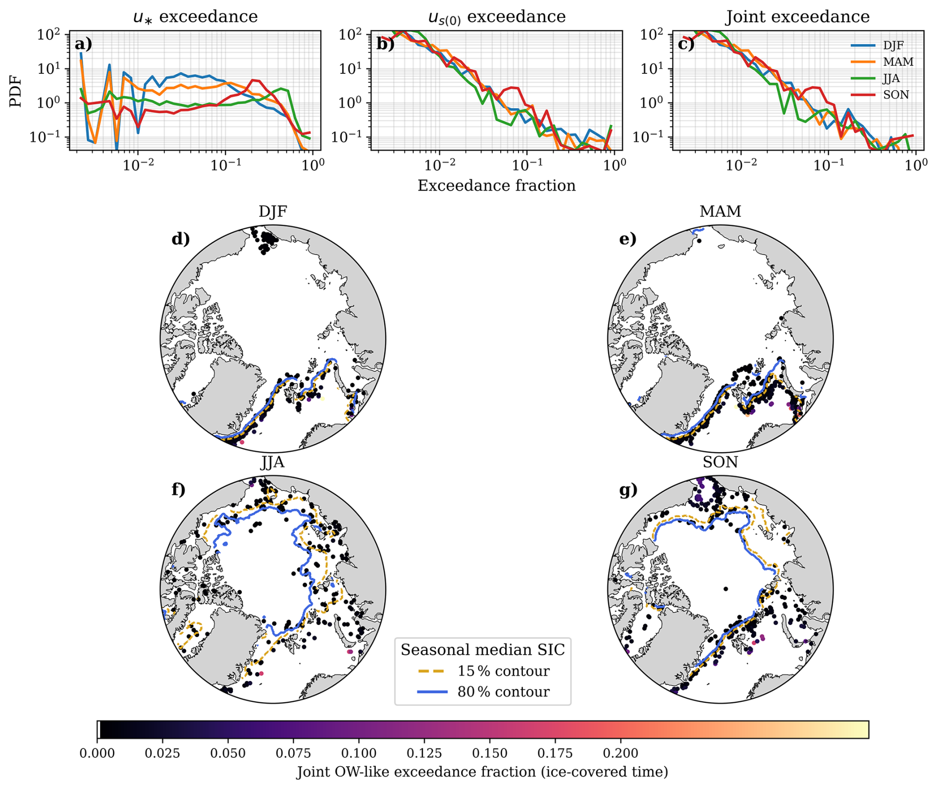
Figure 1 Seasonal exceedance of wind–wave surface forcing beneath Arctic sea ice. (a–c) Probability density functions (PDFs) of exceedance fractions for surface friction velocity (u_*), surface Stokes drift (u_s(0)), and their joint occurrence, computed over ice-covered conditions (SIC≥0.15) relative to seasonal open-water medians (SIC<0.15). (d–g) Spatial distribution of the joint exceedance fraction, defined as the fraction of under-ice time during which both u_* and u_s(0) simultaneously exceed their respective seasonal open-water medians. Elevated values (yellow–orange) indicate regions where wind and wave forcing intermittently reach open-ocean–like magnitudes despite the presence of sea ice. Dashed and solid contours denote the seasonal median 15 % (gold) and 80 % (blue) sea ice concentration boundaries, respectively, providing context for the marginal ice zone and consolidated pack ice. Joint exceedance is shown only at grid cells that experience sea ice conditions at least once during each season.

Spatially (Fig. 1d–g), joint exceedance is concentrated along the MIZ, closely aligned with the 15 %–80 % SIC contours. The highest occurrence is found in the Barents, Greenland, and Chukchi Seas, where fragmented, mobile ice reduces wave attenuation and allows intermittent penetration of wave energy into the ice-covered ocean. Because the OW benchmark is defined separately for each season, exceedance represents a measure of relative forcing intensity rather than absolute magnitude. Across all seasons, joint exceedance remains limited, rarely exceeding 0.2, indicating that simultaneous strong wind and wave forcing beneath sea ice is uncommon. Seasonal differences therefore reflect both variations in forcing and shifts in the reference state. During winter and transitional seasons (DJF, MAM, SON), exceedance is more spatially continuous along the MIZ, consistent with enhanced wave–ice interaction under storm-driven conditions. However, winter shows comparatively low exceedance despite strong winds and wave heights, because the open-water reference state is also elevated, raising the threshold for exceedance. In contrast, fall (SON) shows the highest frequency of elevated joint exceedance values, even though wave heights are more moderate than in winter (Fig. S2). This reflects the combination of a lower open-water reference and more efficient wave penetration into fragmented ice cover, allowing sea ice conditions to more frequently approach OW forcing. Summer (JJA) shows a different regime. Weaker open-water winds and waves reduce the seasonal benchmark, such that moderate forcing more readily exceeds the reference. As a result, exceedance is spatially widespread. However, the magnitude of exceedance remains low, indicating that this broad signal corresponds to weak LT-relevant forcing.

Based on the exceedance metrics, LT-relevant mixing is primarily controlled by the availability and intermittency of wave forcing. Limited wave penetration beneath sea ice suppresses Stokes drift and inhibits LT, favoring predominantly shear-driven mixing, while episodic storm-driven events in the MIZ can temporarily establish open-water-like forcing beneath the ice.

3.2 Mapping upper-ocean mixing regime dynamics in the Arctic

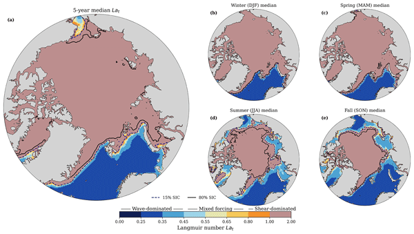
To further explore the controls on LT mixing potential, we examine the spatial and seasonal structure of the turbulent Langmuir number (La_t). All La_t medians are computed over the full spatial domain shown in Fig. 2, without restricting the analysis based on sea ice concentration. The five-year climatological median (Fig. 2a) reveals a persistent band of low La_t encircling the perennial ice pack and closely following the climatological 15 % SIC contour and consistent with patterns shown in Fig. 1. Elevated median La_t values (>1) dominate the central Arctic under compact ice cover, indicating a shear-dominated mixing regime with limited wave influence. In contrast, moderate to low median La_t values (<0.45), which show LT mixing potential, are confined to narrow, seasonally evolving bands along the ice edge. In OW conditions (SIC <0.15), median La_t values are generally below 0.35, consistent with the range identified by Belcher et al. (2012) as favorable for LT mixing. The spatial and seasonal patterns in La_t closely reflect the exceedance statistics, reinforcing that wave-driven mixing is intermittent and strongly modulated by the sea ice cover. As ice concentration increases, wave attenuation limits Stokes-driven forcing, shifting the balance toward shear-dominated mixing and reducing LT mixing potential.

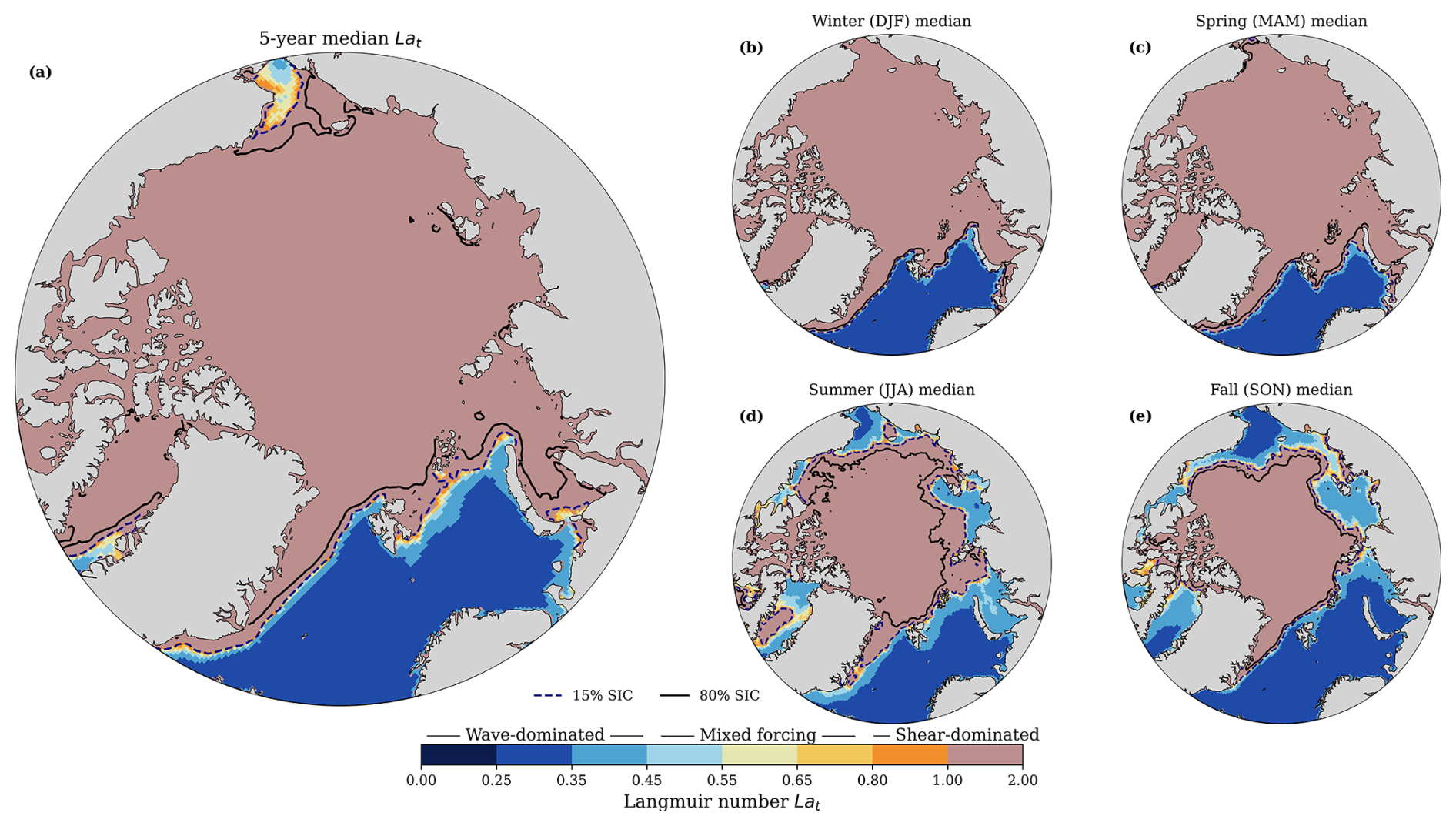
Figure 2 Spatial distribution of the median Langmuir number La_t, integrated over 2018 to 2022, along with its seasonal medians. Panel (a) shows the five-year climatological median of the Langmuir number La_t computed across all seasons. The median 15 % and 80 % SIC contours are overlaid in dashed dark blue and solid black lines marking the median SIC-defined extent of the MIZ across seasons. Panels (b)–(e) show the medians for winter (DJF), spring (MAM), summer (JJA), and fall (SON), respectively. In all panels, La_t is shown for all ocean grid cells without applying a SIC mask; SIC contours are overlaid for context.

Seasonal medians (Fig. 2b–e) further depict how transitions in ice state modulate the balance between wave and wind forcing. During winter and spring (Fig. 2b–c), sharp gradients in La_t delineate the transition from wave-influenced conditions near the ice edge to shear-dominated regimes within the consolidated ice. Compact ice cover strongly attenuates wave energy, limiting the penetration of Stokes drift in ice-covered regions, even under periods of strong wind forcing. In contrast, summer and fall (Fig. 2d–e) show a broader and more continuous band of reduced La_t extending into the seasonal sea ice zone. Lower ice concentration and increased ice mobility can reduce wave attenuation and allow wave-driven forcing to extend farther into the seasonal MIZ, even without stronger wave conditions. These patterns reinforce that departures from open-ocean La_t values are primarily associated with modulation of Stokes drift by sea ice combined with changes in wind forcing. The seasonal MIZ emerges as a distinct transition zone, where the balance between shear- and wave-driven turbulence can shift toward Langmuir-favorable conditions, while the interior pack remains persistently shear-dominated year-round.

Figure 3 synthesizes the spatial structure, temporal variability, and persistence of upper-ocean mixing regimes under ice-covered conditions (SIC≥0.15), based on the regime classification defined in Eq. (12) and the transition framework described in Eqs. (13)–(16). Panel (a) shows the dominant mixing regime at each grid cell, defined as the regime occurring for at least 50 % of ice-covered time. The Arctic interior is characterized primarily by shear-driven mixing (La_t≥0.94), while mixed ($\mathrm{0.43}\le L{a}_{\mathrm{t}}<\mathrm{0.94}$) and wave-driven (La_t<0.43) regimes are confined to the seasonal MIZ and regions near the ice edge, where wind and wave forcing increasingly compete. Panel (c) maps the normalized frequency of regime transitions, expressed as the number of regime changes per ice-covered day. Enhanced regime instability is strongly localized within the MIZ, particularly along sectors exposed to episodic wave activity and intermittent OW conditions. This spatial pattern is consistent with fetch-limited wave growth in partial ice cover, where intermittent Stokes drift enhances variability in the relative balance between wind and wave forcing (Brenner and Horvat, 2024). In contrast, pack ice has uniformly low transition rates, indicating stable and persistent forcing conditions. Localized transitions within consolidated ice likely reflect episodic openings (e.g., leads and polynyas) that temporarily allow wave generation and induce short-lived shifts in mixing regime.

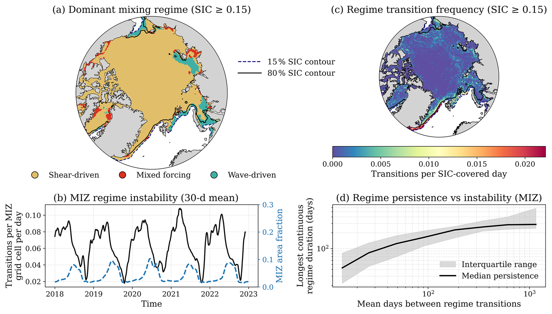
Figure 3 Spatial and temporal characteristics of upper-ocean mixing regime dynamics under sea ice for SIC ≥ 0.15. (a) Dominant mixing regime defined as the regime occupying at least 50% of SIC-covered days at each grid cell over the analysis period. Shear-driven conditions dominate the compact ice interior, while mixed and wave-driven regimes preferentially occur near the ice edge and in seasonally ice-covered regions. Dashed and solid contours indicate the 15 % and 80 % sea ice concentration (SIC) thresholds, respectively. (b) Time series of marginal ice zone (MIZ; 0.15 ≤ SIC ≤ 0.8) regime instability, defined as the fraction of MIZ grid cells undergoing at least one regime transition within a 30 d window (black), together with the contemporaneous fraction of the Arctic domain classified as MIZ (blue, dashed). (c) Normalized regime transition frequency (transitions per SIC-covered day) for SIC ≥ 0.15, highlighting enhanced temporal variability along the MIZ and reduced variability within the compact ice interior. (d) Relationship between regime persistence and instability within the MIZ, shown as the median longest continuous regime duration (black) and interquartile range (shading) binned by the mean number of days between regime transitions. Increasing transition frequency is associated with a systematic reduction in regime persistence.

Panels (b) and (d), restricted to MIZ grid cells ($\mathrm{0.15}\le \mathrm{SIC}\le \mathrm{0.8}$), further resolve the temporal characteristics of regime variability. Regime instability (panel b), defined as the fraction of MIZ grid cells undergoing at least one transition within a 30 d window, reveals a pronounced seasonal cycle with peaks during periods of ice advance and retreat. These peaks precede maxima in MIZ area, indicating that enhanced regime variability occurs prior to, rather than as a consequence of, MIZ expansion. This behavior is consistent with wind, wave, and ice forcing becoming comparable during seasonal transitions in the MIZ, such that no single regime dominates. Small variations in forcing can shift the balance between regimes, leading to frequent transitions and elevated instability along the evolving MIZ boundary. Panel (d) relates regime instability to persistence by comparing the mean time between regime transitions with the longest continuous duration of a single regime within MIZ grid cells. Median regime persistence increases with increasing inter-transition time, although the relationship is nonlinear. Persistence rises rapidly at short timescales before approaching a plateau at longer intervals, with the transition occurring at inter-transition timescales of approximately several weeks (∼ 20–50 d), depending on location within the MIZ. The broad interquartile range at short transition intervals reflects substantial variability in intermittently forced regions near the ice edge, where regimes are frequently disrupted. In contrast, longer transition intervals correspond to more sustained and dynamically stable regimes. Peak instability (∼ 0.1 transitions per day) corresponds to approximately 2–3 transitions per month, with mean intervals of ∼ 10–30 d between transitions. Despite this relatively frequent switching, individual regimes persist for ∼ 50–150 d, increasing to ∼ 100–200 d under low transition frequencies. Overall, this indicates that MIZ uper ocean mixing is characterized by intermittent regime shifts superimposed on otherwise persistent states, rather than continuous or rapid switching, with regime evolution occurring on sub-seasonal timescales.

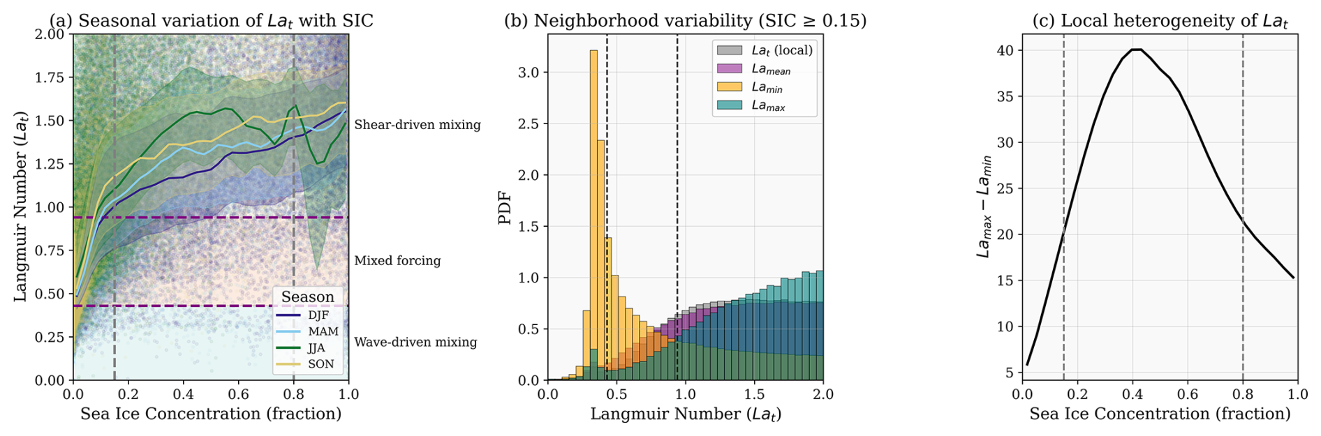
Figure 4 Langmuir number dependence on sea ice concentration and spatial variability. (a) Parametric relationship between La_t and binned sea ice concentration (SIC). Solid lines denote the seasonal median within each SIC bin, with shading indicating interquartile ranges. Purple dashed lines mark the wave-dominated (La_t<0.43) and shear-dominated (La_t>0.94) regime thresholds. (b) Normalized histograms of La_t computed from local grid-cell values and 3×3 neighborhood statistics (mean, minimum, and maximum), aggregated over all ice-covered grid cells (SIC≥0.15). (c) Median local heterogeneity in La_t, defined as $L{a}_{t,max}-L{a}_{t,min}$ within 3×3 neighborhoods, as a function of SIC.

Figure 4 provides complementary insight into how both local and spatially aggregated values of La_t depend on SIC, and helps contextualize the spatial regime structure from in Fig. 3. Panel (a) shows that median La_t generally increases with SIC across all seasons, indicating a systematic shift toward shear-dominated mixing as ice cover increases. Conditions associated with strong LT mixing potential (La_t<0.43) are largely confined to OW or low SIC, whereas shear-dominated regimes (La_t>0.94) dominate at moderate to high SIC. This behavior is consistent with increasing attenuation of wave energy and reduced Stokes drift under higher ice concentrations. During summer, however, the relationship deviates from this monotonic trend. At high SIC (≳0.8), median La_t decreases, indicating a relative increase in wave influence despite high ice concentration. Additional diagnostics (Fig. S3) show that in this regime La_t exhibits limited dependence on sea ice thickness, but decreases rapidly with increasing significant wave height (h_s) over the range 0–1 m. This suggests enhanced sensitivity of La_t to wave forcing, where even modest increases in wave height can substantially increase Stokes drift and reduce La_t. This is consistent with melt-season conditions in which the ice cover becomes mechanically weakened and increasingly spatially heterogeneous. Partial fragmentation and floe-scale openings allow intermittent wave transmission or local, fetch-limited wave generation, while spatial variability in wind stress over melting ice may reduce shear-driven turbulence. Although these processes are not explicitly resolved at model resolution, the results indicate that wave forcing can remain dynamically relevant even at high SIC. In this context, SIC provides a first-order constraint on mixing regimes, but does not uniquely determine the relative importance of wave-driven turbulence during the melt season.

Panel (b) highlights the role of local spatial variability by showing the distribution of La_t within 3×3 grid-cell neighborhoods. The distributions of $L{a}_{\mathrm{t}}^{min}$, $L{a}_{\mathrm{t}}^{\mathrm{mean}}$, and $L{a}_{\mathrm{t}}^{max}$ demonstrate that a wide range of mixing states can coexist locally, even under similar SIC conditions. In particular, $L{a}_{\mathrm{t}}^{min}$ captures the most wave-influenced conditions within a neighborhood, while $L{a}_{\mathrm{t}}^{max}$ reflects the most shear-dominated state. The large spread between these values indicates strong heterogeneity in wave and shear forcing, consistent with a dynamic ice cover containing a mixture of wave-active and wave-suppressed regions. Panel (c) further quantifies this heterogeneity as the difference between local maximum and minimum La_t within each neighborhood. Heterogeneity increases from low SIC and peaks within the MIZ (SIC ≈ 0.3–0.5), reflecting the coexistence of wave- and shear-dominated regimes. At higher SIC, heterogeneity decreases, indicating a transition toward more spatially uniform forcing conditions. Overall, these show that while SIC governs the large-scale transition between mixing regimes, the realized La_t within a given SIC range depends strongly on local ice structure. Fragmentation and spatial heterogeneity in sea ice conditions modulate the intermittency of wave forcing, resulting in highly variable mixing conditions.

3.3 Pan-Arctic dissipation rates and seasonality

Mechanically driven dissipation provides a bulk measure of wind and wave energy input to the upper ocean and complements the regime-based analysis of LT. In our framework, ε_mech quantifies the magnitude of mechanically mediated energy input, while La_t determines how this energy is partitioned between shear- and wave-driven processes. Figure 5a shows that the spatial distribution of median ε_mech is strongly structured by surface forcing, with enhanced dissipation along the MIZ and in peripheral seas exposed to open-ocean winds and wave activity. In contrast, the central pack ice exhibits lower dissipation, consistent with reduced momentum transfer and attenuated wave forcing beneath consolidated ice. This pattern reflects the large-scale distribution of mechanically driven energy input and highlights regions where wind–wave forcing recurrently couples to the upper ocean. Panel (b) shows dissipation intermittency, defined as ${\log }_{\mathrm{10}}(P_{\mathrm{90}}/\mathrm{median})$ of ε_mech, where the 90th percentile and median are computed from the temporal distribution at each grid cell. This metric quantifies the relative importance of extreme events compared to the background state. High intermittency is strongly localized to narrow MIZ regions and ice-edge corridors, indicating that dissipation in these areas is dominated by episodic events. In contrast, regions with elevated median dissipation but low intermittency reflect more persistent, but still moderate, energy input.

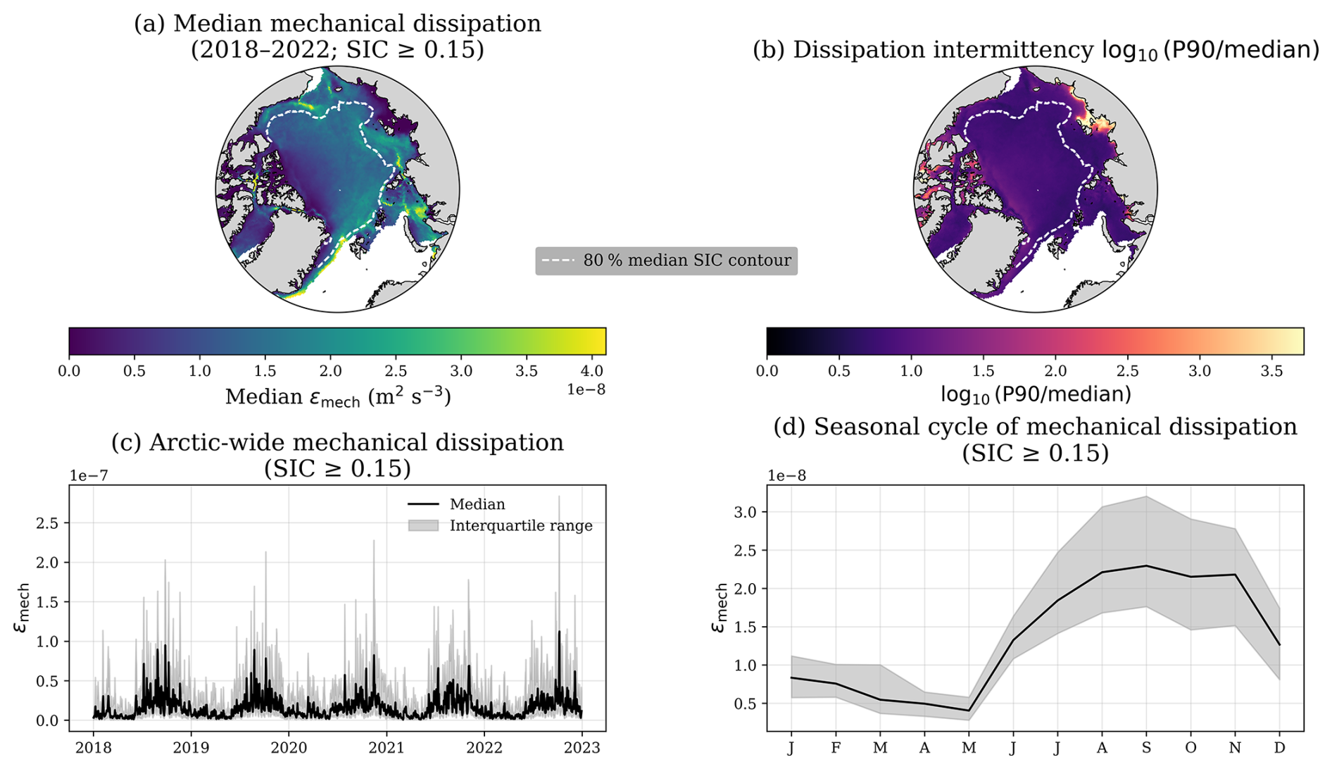
Figure 5 Mechanical dissipation magnitude and intermittency within the Arctic marginal ice zone (2018–2022). (a) Spatial distribution of the aggregated median mechanically forced dissipation, ε_mech, evaluated for ice-covered conditions (SIC ≥ 0.15). (b) Dissipation intermittency index, defined as ${\log }_{\mathrm{10}}(\mathrm{P}\mathrm{90}/\mathrm{median})$ of ε_mech. (c) Arctic-wide temporal evolution of mechanically forced dissipation aggregated over all grid cells classified as MIZ (SIC ≥ 0.15), shown as the spatial median (black line) with interquartile range (shading), illustrating the strongly intermittent nature of MIZ energy input. (d) Seasonal cycle of mechanically forced dissipation within the MIZ, constructed from the monthly climatology of the spatial median in panel (c), with shading indicating the interquartile range.

The spatial correspondence between highly intermittent dissipation and regime-transition hotspots suggests that frequent mixing-regime changes arise where wind-, wave-, and ice-mediated forcing alternately dominate on short timescales. This link is further supported by the Arctic-wide time series in panel (c), which shows that variability in ε_mech is driven by intermittent extremes superimposed on a low median background. The large interquartile range relative to the median indicates that rare, high-energy events contribute disproportionately to temporal variability. This indicates that mechanical dissipation in the Arctic is not controlled by the mean state, but by intermittent high-energy events that dominate variability. Panel (d) shows that dissipation is strongly modulated by season, with peaks in late summer and early autumn and a minimum during late winter under consolidated ice. This seasonal cycle reflects the combined influence of increasing wind stress, reduced ice cover, and enhanced wave activity, all of which act to amplify mechanical energy input into the mixed layer. In the MIZ, mean forcing sets the spatial structure of dissipation, while intermittent events control its variability.

3.4 Impact of wind–wave misalignment on Langmuir turbulence efficiency

The contribution of wave-induced forcing to upper-ocean mixing depends not only on wave strength but also on the relative alignment between wind and waves. To quantify how directional misalignment modulates LT mixing potential, we compare wind-aligned and dynamically projected Langmuir metrics across the Arctic. Misalignment variability is evaluated using the temporal standard deviation of the log-ratio between projected and aligned Langmuir numbers, ${\mathit{\sigma }}_t\left[\log \right(L{a}_{\mathrm{proj}}/L{a}_{\mathrm{t}}\left)\right]$, which captures fluctuations in the effective projection of Stokes forcing onto the Langmuir cell axis. Pan-Arctic spatial patterns (Fig. 6a) show that variability in the projected-to-aligned Langmuir number ratio ranges from approximately 0.05 to 0.30, with the largest values confined to the MIZ, particularly in regions of persistent wave–ice interaction such as the Barents and Greenland Seas. In contrast, the central Arctic exhibits consistently low variability (≲0.1), reflecting weak wave forcing in compact ice cover. Despite this pronounced spatial variability in diagnostic LT metrics, the impact on LT energetics is limited. The 90th percentile change in VKE (Fig. 6b) remains below ∼ 1 % across most of the ice-covered Arctic and exceeds 4 %–6 % only in localized regions near the ice edge. These regions correspond to partial ice cover and active wave propagation, where Stokes drift is sufficiently strong for directional effects to influence the projected shear. These magnitudes indicate that although misalignment can significantly perturb diagnostic LT metrics, its effect on the resulting mixing is comparatively weak.

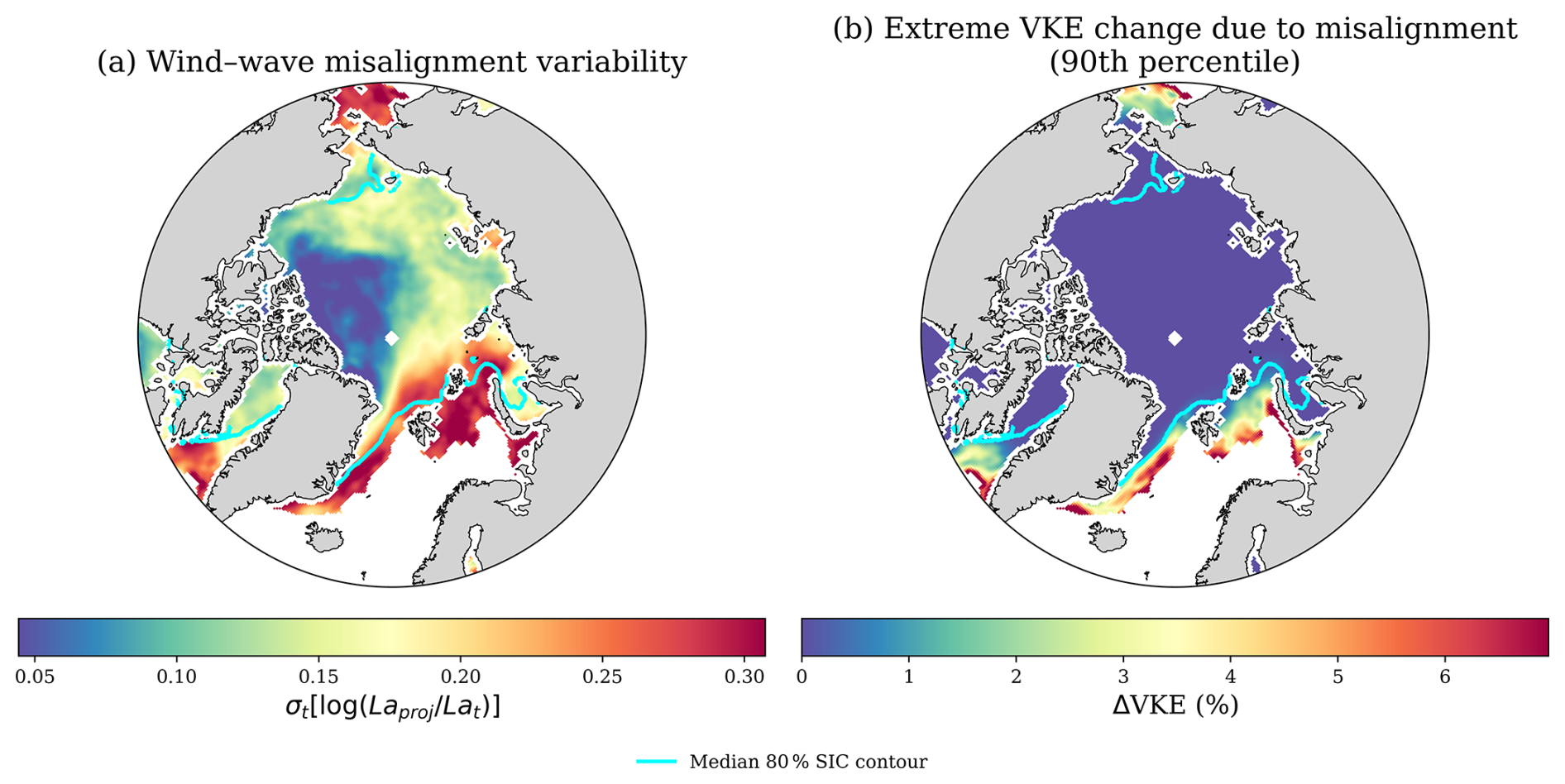
Figure 6 Impact of wind–wave misalignment on Langmuir turbulence across the Arctic. (a) Spatial variability of the projected-to-aligned Langmuir number ratio, expressed as the temporal standard deviation ${\mathit{\sigma }}_t\left[\log \right(L{a}_{\mathrm{proj}}/L{a}_{\mathrm{t}}\left)\right]$, showing regions where wind–wave misalignment most strongly modulates LT diagnostics. (b) Corresponding impact of misalignment on LT energetics, shown as the 90th percentile change in normalized vertical kinetic energy (ΔVKE, %), indicating the upper bound of misalignment effects. The cyan contour denotes the median 80 % sea ice concentration.

To assess how frequently wind–wave misalignment occurs and how it relates to LT variability, we examine the distribution of misalignment angles together with their co-occurrence with wave forcing and the resulting LT response (Fig. 7). The angle distribution (Fig. 7a) shows that moderate-to-large misalignment is relatively common, with more than half of cases exceeding ∼ 30°. However, the joint distribution with wave strength (Fig. 7b) indicates that these larger angles are most often associated with relatively weak wave forcing. The energetic response remains small across all angles (Fig. 7c), with changes in VKE close to zero in most cases and only limited variability at larger misalignment. These suggest that variability in projected LT metrics does not translate directly into changes in mixing, and that the influence of misalignment on LT is secondary compared to variations in wave forcing.

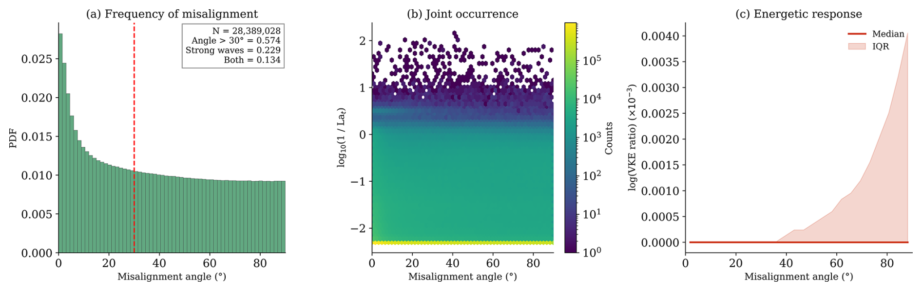
Figure 7 Frequency and impact of wind–wave misalignment on Langmuir turbulence (LT). (a) Probability density function (PDF) of wind–wave misalignment angles for all ice-covered conditions (SIC≥0.15). The dashed line indicates a threshold of 30°, used to distinguish moderate-to-large misalignment. Values inset in the panel show the fraction of samples exceeding the angle threshold, the fraction associated with relatively strong wave forcing (upper quartile of $\mathrm{1}/L{a}_{\mathrm{t}}$), and the fraction satisfying both conditions simultaneously. (b) Joint distribution of misalignment angle and relative wave forcing, represented by ${\log }_{\mathrm{10}}(\mathrm{1}/L{a}_{\mathrm{t}})$, with color indicating occurrence counts. (c) Energetic response to misalignment, expressed as the median log-ratio of vertical kinetic energy (VKE) computed with and without directional effects, shown as a function of misalignment angle. Shading denotes the interquartile range (IQR).

4 Discussion and Conclusions

We used a coupled sea ice–wave modeling framework to quantify the controls on LT mixing potential across the Arctic basin. We show that LT-relevant forcing is fundamentally wave-limited, with Stokes drift strongly attenuated beneath sea ice despite frequent wind forcing of OW magnitude. Favorable conditions for LT mixing are intermittent and largely confined to the MIZ, while the interior pack ice remains persistently shear-dominated. Mixing regimes showed clear spatial and temporal organization, with intermittent, event-driven transitions concentrated in the MIZ, superimposed on otherwise persistent seasonal states. We further demonstrate that SIC alone does not uniquely determine LT forcing, as local wave conditions and ice heterogeneity modulate the balance between shear- and wave-driven turbulence. Finally, we show that while wind–wave misalignment introduces substantial variability in diagnostic LT metrics, its impact on mixing remains small, indicating that LT efficiency is controlled primarily by the magnitude of wave forcing rather than its orientation. This work provides a coherent framework for interpreting the spatial and temporal structure of LT mixing potential across the Arctic, highlighting the following key findings.

4.1 The marginal ice zone as a dynamically distinct mixing regime

The MIZ emerges not simply as a geometric transition zone, but as a dynamically distinct mixing regime in which wave, wind, and ice processes interact to produce intermittent LT forcing. While conditions resembling open-water forcing occur primarily within the MIZ, LT activity is not controlled by MIZ extent alone. Instead, it is governed by the intensity and coherence of wind–wave forcing, which varies seasonally and episodically. As a result, periods of broad MIZ coverage do not necessarily correspond to enhanced LT activity, whereas dynamically active ice-edge regions can support strong, transient LT forcing. The mixing regime-based analysis further shows that LT variability is closely linked to threshold behavior between shear-, mixed-, and wave-dominated states. Regime instability peaks where grid cells frequently cross these physically defined boundaries, indicating that mixing variability arises from fluctuations in forcing that shift the balance between competing processes, rather than from large-scale ice extent alone. This highlights the MIZ as a region of enhanced variability and frequent reorganization of surface forcing, where LT emerges intermittently in response to episodic wave–ice interaction. This behavior extends earlier work showing that ice-edge variability is governed by dynamical thresholds rather than ice extent alone (Horvat et al., 2016).

4.2 Sea ice regulation of Stokes drift and Langmuir turbulence mixing potential

SIC provides a first-order constraint on the mean balance between wave- and shear-driven turbulence by regulating the attenuation of Stokes drift. For most seasons, median La_t increases with SIC, reflecting the progressive suppression of wave-driven forcing relative to wind stress as ice cover increases. This leads to predominantly shear-dominated conditions in the central Arctic. However, SIC alone does not fully explain the variability in LT forcing. Significant departures from the mean SIC–La_t relationship arise across seasons, indicating that additional processes modulate the realized balance between wave and shear forcing. In particular, reduced La_t at higher SIC during summer reflects intermittent wave penetration enabled by thinner, more fragmented ice and enhanced floe-scale heterogeneity. Under these conditions, long-period swell can episodically access nominally ice-covered regions, temporarily enhancing Stokes drift without establishing sustained wave-driven mixing. This indicates that SIC constrains the background forcing state but does not capture the processes that govern LT variability and intermittency.

4.3 Energetics and the role of misalignment

Energetic metrics show that variability in LT mixing is governed primarily by the intermittency of mechanical forcing rather than its mean magnitude. Highly intermittent dissipation is strongly localized to the same MIZ corridors that exhibit frequent regime transitions, indicating that episodic events, such as storms and transient wave penetration, dominate the temporal evolution of mixing. This behavior is consistent with previous studies showing that turbulent mixing in both open-ocean and ice-covered environments is controlled by intermittent, high-energy events rather than by time-mean forcing (Belcher et al., 2012; McWilliams, 2016; Ardhuin et al., 2016; Thomson, 2022; Boutin et al., 2022). Wind–wave misalignment introduces an additional geometric constraint on LT efficiency by reducing the effective projection of Stokes shear onto the Langmuir cell axis. While spatial diagnostics indicate substantial variability in projected LT metrics, the statistical analysis of misalignment angles shows that near-aligned conditions dominate, with most angles below ∼ 30°, and larger misalignment occurring primarily in the MIZ. The energetic response to misalignment is weak. Hence, despite misalignment perturbing LT metrics, its effect on mixing is secondary, with typical changes in VKE remaining small relative to variability driven by wave forcing. LT energetics are controlled primarily by the magnitude and intermittency of wave forcing, while geometric effects act only as a weak modulation. In summary, LT in the Arctic is primarily controlled by intermittent wave forcing within the MIZ, with sea ice setting the background state and misalignment playing a secondary role.

4.4 Implications for Arctic mixed layer dynamics and model development

Our results show that LT in the Arctic is strongly constrained by wave–ice interactions. Wave attenuation beneath consolidated ice limits Stokes drift and confines wave-driven mixing primarily to the MIZ. Thus, parameterizations based on open-ocean conditions are likely to overestimate both the extent and persistence of Langmuir-driven mixing in ice-covered regions. LT forcing is also highly intermittent, driven by episodic wind–wave events along the evolving ice edge. Capturing this variability requires parameterizations that respond to changes in Stokes drift, rather than relying solely on bulk ice properties or steady forcing assumptions. In contrast, wind–wave misalignment plays a secondary role. Although it modifies diagnostic LT metrics, its effect on energetics is small relative to variability associated with wave forcing. These results suggest that improving the representation of wave attenuation and Stokes drift under sea ice is more important than explicitly resolving directional effects for modeling Arctic mixed-layer dynamics.

4.5 Limitations and future directions

Our approach is based on bulk diagnostics and empirically derived scalings and therefore carries several important limitations. The use of ∼ 25 km resolution fields limits our ability to resolve fine-scale processes such as submesoscale eddies, floe-scale wave attenuation, and narrow leads and polynyas, all of which can locally modulate LT and upper-ocean mixing. While neighborhood-based statistics partially capture local heterogeneity, direct assessment of these processes requires higher-resolution modeling and targeted in situ observations. In addition, our analysis relies on a coupled sea ice–wave framework in which the ocean mixed layer does not respond dynamically to wind–wave forcing, and stratification feedbacks are not explicitly resolved. Mixed-layer depth and buoyancy effects are prescribed, limiting the realism of the diagnosed vertical mixing response. In particular, buoyancy-driven convection and LT are expected to interact nonlinearly in ice-covered and meltwater-influenced environments, yet their relative contributions remain poorly constrained. As a result, the metrics presented here should be interpreted as indicators of LT mixing potential, rather than predictions of realized turbulent states.

Addressing these challenges ultimately requires fully coupled ocean–wave–ice models that resolve stratification, wave propagation beneath ice, and wind–wave misalignment simultaneously. Recent and ongoing studies are beginning to resolve Langmuir turbulence under partially ice-covered and weakly stratified regimes using large-eddy simulations, regional modeling, and coordinated observations (e.g., Brenner et al., 2023; Lee et al., 2025). These efforts provide a clear pathway toward stratification-aware, ice-modified Langmuir parameterizations.

Complementary observational efforts are also essential. Coordinated field campaigns employing autonomous profilers, SWIFT drifters, and satellite altimetry will be critical for evaluating Langmuir diagnostics and parameterizations in ice-covered waters. In particular, observational and modeling studies should prioritize the MIZ, where wave–ice–wind interactions are most dynamically active. Finally, quantifying the impact of LT on vertical tracer transport, stratification erosion, and ice–ocean heat exchange in climate models will be essential for assessing its broader role in the evolving Arctic system.