Radiostratigraphy and surface accumulation history of the Amundsen-Weddell Ice Divide, West Antarctica

Recent ground-based radio-echo sounding (RES) surveys conducted by Centro de Estudios Cientificos (CECs) across the Ellsworth Subglacial Highlands (ESH), a topographically complex region near the Amundsen–Weddell ice divide (AWID), reveal new insights into Holocene accumulation and constrains the ice flow stability near AWID. We traced seven Internal Reflection Horizons (IRHs) across approximately 2000 km of RES data spanning a 13 000 km² area in the upper catchments of Pine Island Glacier, and the Rutford and Institute Ice Streams. Two of these IRHs intersect dated airborne radar lines tied to the WAIS Divide 2014 (WAISD-2014) ice-core chronology. Applying the Dansgaard–Johnsen model with local accumulation rates from stake measurements and satellite-derived values we estimated ages of up to ∼ 17.6 kyr for the deepest horizon (IRH7). Internal stratigraphy is well preserved in the slow-flowing alpine terrain of the ESH but becomes disrupted in areas of relatively fast flow and tributary convergence, such as the southern Ellsworth and CECs troughs. Despite these localised disturbances, IRHs remain traceable across most of the region, highlighting the potential for radiostratigraphic continuity in complex settings. Modern and Holocene accumulation patterns reveal a persistent asymmetry across the AWID, with consistently higher accumulation in the CECs Trough, supporting long-term ice divide stability since at least the mid-Holocene. Our study extends the spatial coverage of dated radiostratigraphy in West Antarctica and provides new linkages between the Weddell and Amundsen Sea Embayments. These results extend dated radiostratigraphy into a previously unresolved sector of West Antarctica, supporting AntArchitecture goals by strengthening continent-scale IRH connectivity, improving constraints on Holocene accumulation variability, and providing new observational benchmarks for ice-sheet models.

1 Introduction

Satellite observations have revealed a significant and ongoing mass loss from the Antarctic Ice Sheet, particularly driven by an acceleration of ice discharge from the Amundsen and Bellingshausen Sea sectors of West Antarctica over the last three decades (e.g., Rignot et al., 2019; Shepherd et al., 2019). Between 1992 and 2020, this region experienced some of the most dynamic changes within the ice sheet system (Otosaka et al., 2023), and has contributed up to 0.3 mm yr⁻¹ to global sea level since 2002 (Groh and Horwath, 2021). It has also been dynamic over longer time periods, with marine geological records indicating progressive grounding-line retreat and temporary standstill positions since the Last Glacial Maximum (LGM) across the Amundsen and Bellingshausen margins (e.g., Hillenbrand et al., 2013; Larter et al., 2014). Further inland, geomorphological, ice-core, and cosmogenic nuclide data have revealed substantial ice-sheet thinning since the LGM (Bentley et al., 2010; Hein et al., 2016a; Grieman et al., 2024). These observations are consistent with numerical modelling results, which suggest strongly heterogeneous and temporally variable dynamic behaviour throughout the West Antarctic Ice Sheet (WAIS) (e.g., Kingslake et al., 2018; Smith et al., 2020).

Despite this widespread evidence of dynamic behaviour, the configuration and position of the Amundsen-Ross and Amundsen–Weddell Ice Divide appear to have remained comparatively stable during the Holocene (Conway and Rasmussen, 2009; Ross et al., 2011). Cosmogenic nuclide data and geomorphological mapping from the southern Ellsworth Mountains suggest that any fluctuations in divide position and ice thickness over the past 1.4 million years were limited in magnitude (Hein et al., 2016b; Small et al., 2025). This contrast, between marked dynamic change in adjacent marine-terminating sectors and apparent long-term stability of the inland divide, raises fundamental questions about the mechanisms of mass redistribution and flow reconfiguration within the WAIS. One means of investigating past flow regimes and ice sheet evolution is through the analysis of internal reflection horizons (IRHs) detected by radio-echo sounding (RES). IRHs arise from contrasts in dielectric properties within the ice column, associated with changes in density, conductivity, and crystal orientation fabric (Clough, 1977; Fujita et al., 1999; Siegert, 1999; Dowdeswell and Evans, 2004; Bingham et al., 2025). Many stratigraphically coherent IRHs originate from atmospheric deposition events such as dust pulses or volcanic eruptions, which introduce conductivity contrasts that become preserved within the ice column (e.g., Hammer, 1980; Lambert et al., 2008; Sigl et al., 2014; Wilson et al., 2022). As such, IRHs provide isochronal surfaces that can be traced across wide areas and, if independently dated, can be used to constrain accumulation rates, infer deformation patterns, and identify basal melting or englacial folding (e.g., Siegert and Payne, 2004; Hindmarsh et al., 2006; Bingham et al., 2015; Holschuh et al., 2018; Jordan et al., 2018; Ashmore et al., 2020; Ross and Siegert, 2020).

Perhaps most critically, IRHs provide a means to propagate deep ice-core age constraints from point locations to regional scales, thereby enabling the construction of ice sheet-wide chronologies and age–depth models (e.g., Karlsson et al., 2012; MacGregor et al., 2015; Cavitte et al., 2016). These stratigraphic datasets are increasingly used to constrain the long-term evolution of ice sheet dynamics and to calibrate numerical ice sheet models, a capability that is increasingly recognised as necessary for reducing uncertainty in projections of future mass balance and sea-level contribution (e.g., Born, 2017; Sutter et al., 2021; Rieckh et al., 2024; Bingham et al., 2025).

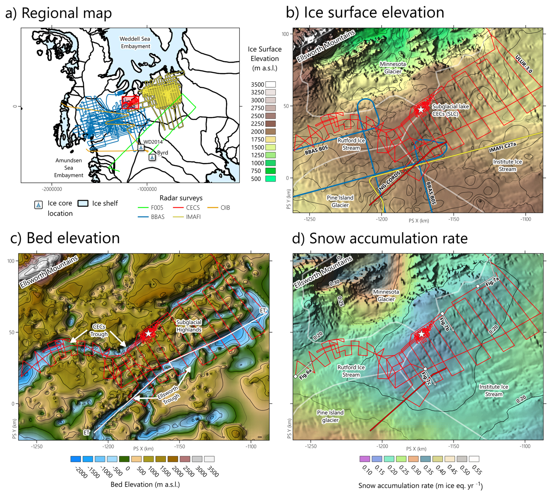
Figure 1 (a) Location of the Ellsworth Subglacial Highlands (ESH) relative to the West Antarctic Ice Sheet (WAIS) and the radio-echo sounding (RES) surveys used in this study. The red box outlines the area shown in panels (b), (c), and (d). Coloured lines indicate different RES campaigns: BBAS in blue (Corr et al., 2021), IMAFI in yellow (Ross et al., 2021), and CECs in red. These campaigns were used to extend the radiostratigraphy from two dated ice cores: Byrd and WAIS Divide (WAISD-2014). (b) Ice surface elevation from BedMachine Antarctica v3 (Morlighem et al., 2020), overlain on the Radarsat Antarctic Mapping Project (RAMP) mosaic (Liu et al., 2015) with black contour lines indicating elevation isolines every 250 m. Coloured lines show the different RES surveys and their intersection along the ice divide between Pine Island Glacier and Institute Ice Stream, as well as in Rutford Ice Stream. (c) CECs RES survey lines across the ESH, shown over basal topography from Napoleoni et al. (2020). Locations of CECs Trough, Ellsworth Trough and Subglacial Highlands are indicated, and RES control lines ET and ET′ (see Fig. 2a) are also highlighted. (d) Snow accumulation rates derived from statistically downscaled regional climate model output (27 to 2 km resolution; Noël et al., 2023), overlain on RAMP imagery with black contour lines indicating accumulation isolines every 0.05 m ice eq. yr⁻¹. The locations of profiles shown in Figs. 6 and 7 are also indicated by white segments with corresponding labels. All panels: White lines denote ice catchment boundaries from the MEaSUREs dataset (Mouginot et al., 2017), and a white star indicates the location of Subglacial Lake CECs (SLC).

While radiostratigraphic studies have constrained internal layer geometry and chronology across parts of the Weddell Sea sector and the Amundsen Sea Embayment (e.g., Karlsson et al., 2014; Ashmore et al., 2020; Bodart et al., 2021), the interior region straddling the Amundsen–Weddell Ice Divide remains sparsely sampled (Fig. 1a). This divide is of particular significance as it encompasses the upper reaches of several major outlet glaciers and ice streams, including Pine Island Glacier (PIG), Thwaites Glacier, Rutford Ice Stream (RIS), and Institute Ice Stream (IIS), whose present and past dynamics exert a dominant control on WAIS mass loss (Fig. 1b).

Beneath this ice divide lies the Ellsworth Subglacial Highlands (ESH; Fig. 1c), a complex landscape characterised by deeply incised valleys and rugged mountainous topography. This terrain likely formed under warmer climatic conditions, potentially associated with dynamic tidewater-style glaciation during past interglacials or pre-Quaternary periods (Ross et al., 2014). The ESH is dissected by major subglacial troughs, including the Ellsworth Trough (ET) and the CECs Trough (CT), which may serve as palaeo-flow corridors and subglacial hydrological pathways linking the Amundsen and Weddell Sea embayments (Vaughan et al., 2011; Siegert et al., 2012; Napoleoni et al., 2020; Pritchard et al., 2025). These topographic features likely influence the routing of basal meltwater and the basal thermal regime, thereby exerting control on past ice divide migration, ice stream switching, and flow reorganisation. Given the hypothesised long-term stability of the ice divide, this region offers a promising setting in which to trace radar stratigraphy across areas of complex basal topography.

The climatic context of this region also suggests spatial heterogeneity in mass balance (e.g. Bodart et al., 2023). While snow accumulation rates in Ellsworth Land appear relatively stable over the past ∼ 3.1 kyr, with values comparable to present-day estimates (Siegert and Payne, 2004), other regions of coastal West Antarctica experienced significant accumulation increases post-1900 (Thomas et al., 2015; Medley and Thomas, 2019), highlighting the importance of establishing region-specific accumulation histories.

In this study, we use ground-based RES data acquired by the Centro de Estudios Científicos (CECs) in 2006 and 2014 to investigate the englacial stratigraphy of the Amundsen–Weddell Ice Divide region.Throughout this work, “CECs” refers to the institution, and as “CECs surveys” to the associated radar datasets. We note that two geographic features within our study region, the CECs Trough (Napoleoni et al., 2020) and Subglacial Lake CECs (SLC; Rivera et al., 2015), are also named after the institution; to avoid confusion, we explicitly refer to these by their full geographic names. The bed topography from these surveys was previously published in Napoleoni et al. (2020) and the data are incorporated in BEDMAP3 (Fremand et al., 2022) but the detailed stratigraphy has not previously been mapped on a regional scale. By tracing and correlating the IRHs across the Ellsworth Subglacial Highlands, we link existing radiostratigraphies from the Amundsen and Weddell Sea sectors and extend dated stratigraphy into a region that was previously poorly constrained. Our specific objectives are to: (1) characterise geometry, continuity, and age of IRHs across the divide; and (2) use these dated IRHs to reconstruct spatial variations in Holocene accumulation and assess their implications for local divide-proximal ice-flow stability, thereby extending previous regional interpretations.

2 Data and methods

We analysed ground-based RES data collected by CECs in 2006 (Vaughan et al., 2006) and 2014 (Rivera et al., 2015) to identify and map seven continuous Internal Reflection Horizons (IRHs) across the upper catchment of Pine Island Glacier (PIG), Rutford Ice Stream (RIS), and Institute Ice Stream (IIS) in the ESH (Fig. 1). We then intersected this newly identified englacial stratigraphy to the existing dated IRHs in IIS (Ashmore et al., 2020), from the British Antarctic Survey (BAS) “IMAFI” survey (Corr et al., 2021; Fig. 1a), and PIG (Bodart et al., 2021) from the BAS “BBAS” survey (Ross et al., 2021; Fig. 1a) to match and estimate the age and accumulation rates for two englacial layers. The existing radiostratigraphy was primarily established with data acquired using airborne RES (Vaughan et al., 2007; Corr et al., 2007) operating at a similar centre frequency (i.e. 150 MHz) to the ground-based CECs system (i.e. 155 MHz). We also applied the model of Dansgaard and Johnsen (1969) to calculate the age of the ESH englacial stratigraphy independently by using a suite of accumulation rates and basal shear thicknesses (see Tables A1, A2, A3). Uncertainties are quantified throughout the process and provide an overall estimation for the age of each IRH. We explain our approach in detail below.

2.1 CECs RES surveys

We used three ground-based RES datasets (Table A5) obtained between 2006 and 2014 by CECs, using two RES systems. The first survey in 2006 acquired ∼ 300 km of along-track data using the 150 MHz centre frequency and pulse-compressed Next Generation Coherent Radar Depth Sounder (NG-CORDS; Gogineni et al., 2001) system. The two subsequent surveys, in January and December 2014, acquired ∼ 1700 km of along-track data using the 155 MHz centre frequency and coherent pulse compression deep-looking RES Ulloa-Uribe 3.0 (ULUR-3.0; Uribe et al., 2014; Rivera et al., 2015). The raw radar data were first pre-processed using background removal, a dewow filter, and gain function adjustment. Coherent integration (2048 traces) was then applied using an unfocused synthetic aperture radar (SAR) approach to reduce oblique scattering, enhance along-track resolution, and improve the signal-to-noise ratio. Finally, Kirchhoff migration was applied prior to manual picking to correct for geometric distortion and improve reflector positioning. The three ground-based surveys (NG-CORDS 2006, ULUR January 2014 and ULUR December 2014), hereafter named the “CECs survey”, were geolocated using dual-frequency Lexon GD GPS receivers (Rivera et al., 2015).

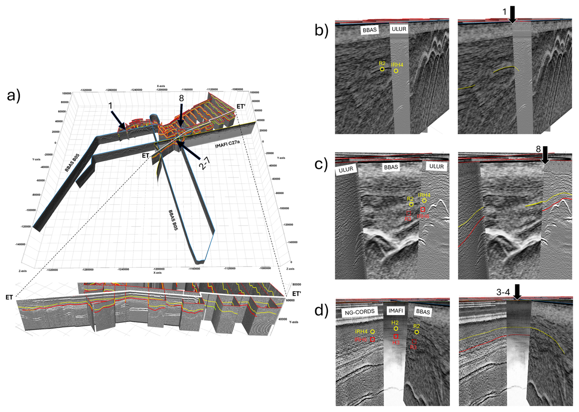
Figure 2 Intersection of the CECs, BBAS, and IMAFI surveys. (a) A 3D view of the surveyed region, showing englacial layers tied to the WAISD-2014 (Bodart et al., 2021) and Byrd ice-core (Ashmore et al., 2020). see Fig. 1a for core locations. Numbers 1–8 mark intersections with previously established radiochronologies in Area 1 (CECs Trough), Area 2 (Subglacial Highlands) and Area 3 (Ellsworth Trough). The profile ET-ET' shows the control line we use to start tracing englacial layers across the study area (location of profile in Fig. 1c). (b) Area 1: Intersection within the CECs trough between the BBAS radar line and the CECs survey, illustrating the continuity of englacial layer R2 and IRH4 in both datasets. (c) Area 2: Intersection in the Subglacial Highlands between the BBAS (R2 and R3) and CECs (IRH4 and IRH6) surveys. (d) Area 3: Intersection within the Ellsworth Trough among the BBAS (R2 and R3), IMAFI (H2 and H3), and NG-CORDS (IRH4 and IRH6). Dashed circle and square indicate the projection of the original IRH to the intersection with the CECs survey.

2.2 IRH tracing and lateral continuity

We used the Schlumberger software Petrel to manually pick and map seven distinctive englacial reflections (IRH1 to IRH7, from the shallowest to the deepest) across all CECs survey with a three-step workflow:

1. We manually picked the greatest amplitude of the most laterally continuous englacial reflections, including cases when a single reflection diverged into several reflections before merging into a single IRH again. To achieve laterally consistent IRHs across the surveyed area, we selected distinctive sets of englacial reflections that could be traced together with greater confidence, using crossovers between CECs surveys to ensure reliability in the tracing process (e.g., Bingham et al., 2025). This approach allowed us to coherently trace the core layer of interest within that package and bridge most of the horizontal gaps in the continuity of the IRHs.

2. We selected the RES lines acquired along the central flow line of ET as reference for this new englacial stratigraphy. Utilising the NG-CORDS survey (Fig. 1) we selected the most prominent and laterally continuous reflections, and then expanded these reflections to the remaining central flow lines acquired during the CECs surveys to intersect this survey with the BBAS and IMAFI surveys (Fig. 1). We found multiple intersections between the BBAS and CECs surveys but only one intersection between CECs and IMAFI Surveys, identifying two layers at similar depth in six intersections between BBAS and CECs surveys, and in two intersection between IMAFI and CECs surveys (Fig. 2). Using the RES lines at each intersection (between CECs, BBAS and IMAFI survey) as vertical tie points for the IRHs we followed each reflection until we were no longer able to distinguish the IRH from the surrounding reflections (e.g., due to large dip angles, excessive buckling of IRHs, or to weak reflections). We excluded the bottom segment (∼ 400 m) of the ice column to avoid any diffuse reflection from the ice-bed interface (e.g., backscattering; Franke et al., 2023), or any potential reorganization of the ice crystals due to shear stress in the basal zone or basal melting (e.g., Fujita et al., 1999; Artemieva, 2022). This way, we could confidently assume that the IRHs we identified in this work were isochronous, and comparable to those intersected with other surveys (e.g., Siegert and Payne, 2004; Karlsson et al., 2014; Ashmore et al., 2020; Bodart et al., 2021).

3. To compare the intersection between the different surveys, we assumed an electromagnetic wave velocity propagation through the ice of 0.1685 m ns⁻¹ to calculate the depth in metres. In addition, to maintain consistency with previous studies in the region (e.g., Ashmore et al., 2020), we applied a spatially uniform firn correction of 10 m across the Ellsworth Subglacial Highlands (ESH), assuming that spatial variability in firn thickness is minor at the scale of our analysis.

We systematically measured the lateral layer persistence along radar transects using the internal layer continuity index (hereafter ILCI), first applied by Karlsson et al. (2012) and subsequently used in others studies in the region (Bingham et al., 2015; Winter et al., 2015; Ashmore et al., 2020). This dimensionless index can be used to interpret disruption in the englacial reflectors continuity as a consequence of – for example – topography, the onset of enhanced ice flow, shear margins, or abrupt changes in the ice flow direction. The index is calculated using un- or minimally-processed radar data and measures the rapidity with which the signal changes between extreme low and high amplitude values (Karlsson et al., 2012). To calculate ILCI, we stacked three consecutive raw traces from radar data to improve the signal-to-noise ratio (SNR), and then set a range within the ice column to be analysed. For the purposes of the ILCI calculation, the upper part of the ice column (U) is defined as the surface to 200 m depth and is excluded because it was sounded with a different radar system (FMCW; Uribe et al., 2017). The lower end of the ice column (L) is defined as the basal 400 m above the ice-bed interface (i.e., the lowest ∼ 400 m of the ice column), which is excluded because internal reflections are weak or absent and bed-related scattering can dominate the return (Drewry and Meldrum, 1978; Drews et al., 2009). Because L is referenced to the bed rather than the surface, the lower bound of the analysed interval occurs at different absolute depths below the surface depending on local ice thickness (e.g., Fig. 4).

Assuming that the total number of samples of reflected power between the surface and the bedrock is M, we defined a subinterval of radar samples (N) as,

$$\begin{array}{}\text{(1)}& N=\left[\right(\mathrm{1}+U):(M-L\left)\right]=[n_{\mathrm{1}}:n_N]\end{array}$$

where U, is defined as the number of samples equivalent to ∼ 200 m; and L, as the number of samples equivalent to 400 m. We then calculated the ILCI index (Ψ) as:

$$\begin{array}{}\text{(2)}& \mathrm{\Psi }={\displaystyle \frac{\mathrm{1}}{\mathrm{2}{\mathrm{\Delta }}_{r}N}}\sum _{i=n_{\mathrm{1}}}^{n_N}|P_{i+\mathrm{1}}-P_{i-\mathrm{1}}|\end{array}$$

where P_i is the reflected relative power (dB) at point i and Δ_r is the depth (m), which is used as a scaling factor (Karlsson et al., 2012). After calculating the ILCI, individual values were averaged horizontally over a moving window of 10 traces. Higher values of ILCI indicate well-preserved englacial reflectors, whereas lower ILCI values characterise sections where englacial reflectors are largely absent.

2.3 Dating and modelling ESH radiostratigraphy

We used two independent approaches to constrain the ages of our IRHs: (1) intersections with previously published radiostratigraphy, and (2) ice-depth modelling.

2.3.1 Intersection with previous radiostratigraphy

Utilising the existing radiostratigraphy previously linked to the WAIS Divide (Bodart et al., 2021) and Byrd ice-core chronologies (Ashmore et al., 2020), we matched the IRHs from the CECs survey to the corresponding IRHs identified in the BBAS and IMAFI survey (Fig. 2), spanning both the Amundsen Sea Embayment (Karlsson et al., 2014; Bodart et al., 2021) and the Weddell Sea Embayment (Siegert and Payne, 2004; Ashmore et al., 2020).

To guide the interpretation of our seven IRHs, we drew upon an established framework of published radiostratigraphy. Prominent reflections were originally identified in profile F005 from the 1977/78 SPRI-NSF-TUD survey (Siegert and Payne, 2004; Bingham et al., 2025) and later observed along the ITASE traverse (Jacobel and Welch, 2005), forming the basis for subsequent regional radiostratigraphic frameworks. These reflections were later linked to englacial Layers 1 and 2 in the Amundsen Sea Embayment by Karlsson et al. (2014), and further extended by subsequent analyses from the BBAS and IMAFI surveys (Bodart et al., 2021; Ashmore et al., 2020).

In the BBAS survey, Bodart et al. (2021) traced four IRHs (R1–R4) across Pine Island Glacier using the 150 MHz centre frequency PASIN-1 RES system (Fremand et al., 2022) and the 190 MHz centre frequency MCoRDS2 RES system (Table 1 in Bodart et al., 2021). Similarly, three reflections (H1–H3) were traced across the Institute and Möller Ice Streams in the IMAFI survey also using the PASIN-1 RES system (Ashmore et al., 2020). Together, these linked datasets provided a consistent age framework based on annual layer counting from chemical, dust, and electrical conductivity records (Sigl et al., 2016; Blunier and Brook, 2001).

In three areas we were able to match two prominent IRHs in our survey (CECs) with those IRHs identified in previous surveys (i.e. BBAS and IMAFI surveys). We first used the BBAS survey to match our IRH2 to R2 at six intersections (intersections 1–3, 5, 7 and 8 in Fig. 2b and c), and our IRH6 to R3 (Bodart et al., 2021) in one intersection across all three areas (intersection 4 in Fig. 2c). We then used the intersection between CECs and IMAFI survey to match our IRRH4 and IRH6 to H2 and H3, respectively, at one intersection in area 3 (intersection 2 in Fig. 2c). These tie-points were used to: (1) assign a preliminary age to IRH4, (2) estimate vertical offsets between the two surveys, and (3) determine local accumulation rates at each area. See Sect. 2.4 for details on uncertainty quantification.

2.3.2 Age-depth modelling

To estimate the age of the five remaining IRHs not directly tied to existing radiostratigraphy (namely IRH1-3, IRH5, and IRH7), we applied a one-dimensional (1-D) Dansgaard–Johnsen (D–J) model (Dansgaard and Johnsen, 1969), testing a range of Holocene and present-day accumulation rates (Fig. 3). To account for uncertainty in past accumulation, we consider a range of plausible accumulation scenarios derived from Noël et al. (2023), Arthern et al. (2006), and snow stake rates. We refer to these as “low-accumulation” and “high-accumulation” scenarios, representing the lower and upper bounds of the accumulation estimates (Tables A1, A2 and A3). These bounds are used to explore the sensitivity of age–depth relationships to accumulation variability. While other models have been developed for estimating IRH ages (e.g. Nye and Perutz, 1957; MacGregor et al., 2015), and more complex methods involving forward modelling of electrical conductivity have been employed in East Antarctica (Franke et al., 2025), we selected the D–J model to maintain consistency with previous studies in this region (e.g. Siegert and Payne, 2004; Jacobel and Welch, 2005; Karlsson et al., 2014; Ashmore et al., 2020; Bodart et al., 2021), and to facilitate direct comparison of IRH-derived age estimates. Moreover, recent findings by Sanderson et al. (2024) suggest other approaches, such as Nye-style modelling applied along the transect between Dome A and the South Pole (characterised by slow, largely steady ice flow, minimal lateral variability in accumulation, and smoothly varying vertical strain rates), can yield age–depth relationships that are broadly comparable to those produced by the D–J model, thereby reinforcing the credibility of this later age-modelling strategy under appropriate conditions.

However, as a sensitivity test that relaxes basal-condition assumptions, we applied a simplified quasi-Nye dating approach (MacGregor et al., 2015) to propagate ages between independently dated internal reflection horizons (IRHs). In quasi-Nye dating, the vertical strain rate is assumed to be uniform within the depth interval bounded by a dated layer pair, so age propagation depends on the relative vertical spacing of IRHs rather than on basal shear-layer parameterisation. We implemented this approach at a representative site 2 where all seven traced IRHs are present and where the horizons IRH4 and IRH6 are independently dated. We used IRH4 (4.72 ± 0.28 kyr) and IRH6 (6.94 ± 0.33 kyr) as age constraints to estimate ages for IRH5 and IRH7 using a quasi-Nye approach. In this framework, ages are propagated between dated layers under the assumption of a constant effective vertical strain rate within the bounded interval, resulting in a physically consistent, non-linear age-depth relationship.

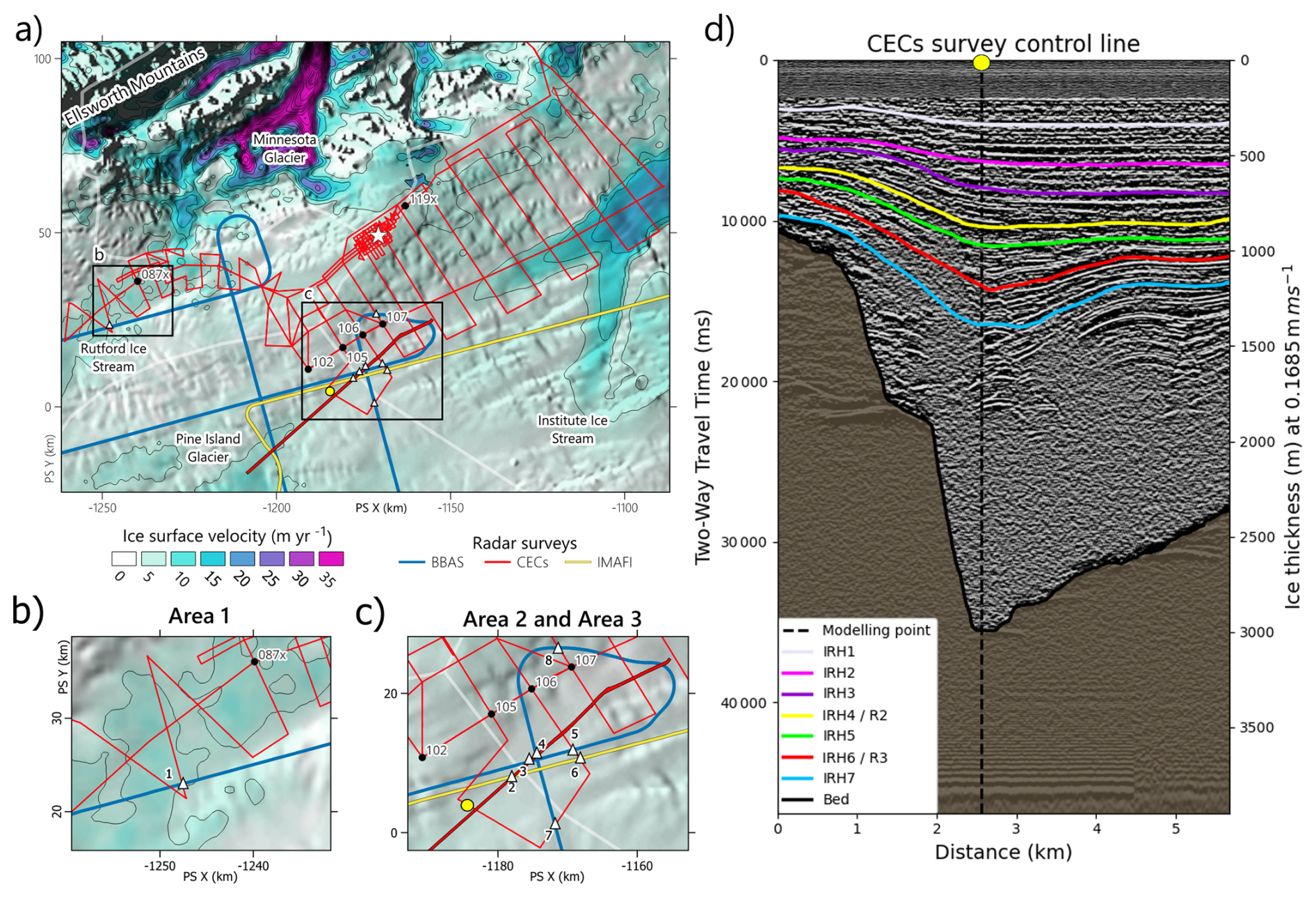
Figure 3 Extension of the Byrd and WAISD 2014 ice-core radiochronology using CECs RES surveys, contextualized by ice surface velocity. (a) CECs survey intersecting BBAS and IMAFI radar lines overlaid on mean annual ice surface velocity (Mouginot et al., 2019) and RAMP imagery (Liu et al., 2015) with black contour lines indicating ice surface velocity isolines every 5 m yr⁻¹. Black dots indicate snow stakes for measuring present-day snow accumulation near intersection sites, with thin black lines showing contours of mean annual ice surface velocity. (b) Intersection in Area 1 between BBAS and CECs surveys in Rutford Ice Stream (see Fig. 3a for location). (c) Intersections in Areas 2 and 3 between BBAS, IMAFI, and CECs surveys near the ice divide between Pine Island Glacier and Institute Ice Stream (see Fig. 3a for location). The yellow circle indicates the position of the trace used to model ice depth chronology for seven internal reflection horizons (IRHs). (d) Radar line crossing the site for ice depth modelling, with the yellow circle marking the same trace from panels (a) and (c) where Internal Reflection Horizon (IRH) depths were obtained. Grey lines in all panels delineate ice catchment boundaries from MEaSUREs (Mouginot et al., 2017).

The D–J model assumes steady-state vertical ice flow, a constant vertical strain rate above a basal shear layer, and no temporal changes in accumulation at the modelled point. The age of an IRH, t (kyr), is given by:

$$\begin{array}{}\text{(3)}& t={\displaystyle \frac{\mathrm{2}H-h}{\mathrm{2}a}}\ln \left({\displaystyle \frac{\mathrm{2}H-h}{\mathrm{2}z-h}}\right),h\le z\le H\end{array}$$

where H is the total ice thickness (m), h is the thickness of the basal shear layer (m), a is the average accumulation rate (m yr⁻¹ ice-equivalent) since deposition of the IRH, and z is the elevation of the IRH above the bed (m). Following the approach of Bodart et al. (2021), we tested basal shear layer thicknesses of 20 %–30 % of the ice column to evaluate model sensitivity.

The basal shear layer thickness ratio ($h/H$) can vary substantially across different flow regimes and ice-sheet settings (e.g., Waddington et al., 2005; MacGregor et al., 2016). In this study, $h/H$ is treated as an uncertainty parameter rather than a fixed quantity, and we restrict our age-depth modelling to locations that best satisfy the assumptions of the D–J framework (low horizontal velocities, locally smooth bed, and laterally coherent stratigraphy). We additionally evaluate the sensitivity of IRH ages to alternative, bed-decoupled age-propagation assumptions using a quasi-Nye approach (Sect. 2.3.3), which provides an independent check on whether uncertainty in basal shear-layer parameterisation materially influences the inferred age structure over the depth interval bounded by the traced IRHs.

We applied the model to the northern sector of ET (upstream of SLE; area 3 in Fig. 3), close to the Amundsen–Weddell Ice Divide. This site has been shown to remain stable throughout the Holocene (Ross et al., 2011; Hein et al., 2016b), making it suitable for D–J style modelling. Although other locally flat bed regions exist within the ESH, they present substantially higher flow speeds (e.g. along the Ellsworth Trough towards the Institute Ice Stream). Our choice therefore reflects a balance between maintaining a relatively flat bed and minimising ice velocity, prioritising slow-flowing divide-proximal ice.

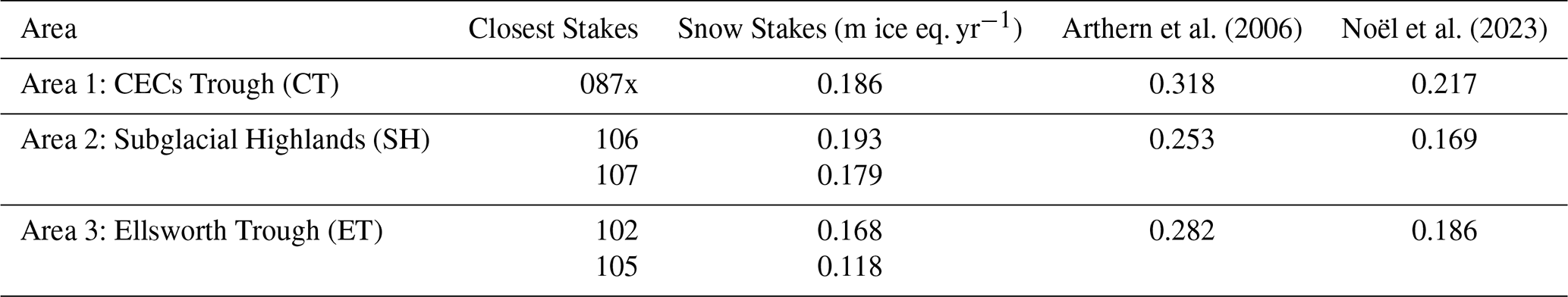
We estimated the Holocene mean accumulation rate, a, using three complementary approaches. First, we used stake-based accumulation measurements collected in 2014 and 2015 (Table 1). These included values from the snow stake closest to area 1 (087×), area 2 (106 and 107) and area 3 (102 and 105) as shown in Fig. 3.

Second, we evaluated accumulation-rate products derived from regional modelling frameworks. Our primary accumulation estimates are based on RACMO2.3p2 (Noël et al., 2023). To assess the sensitivity of inferred IRH depths and ages to uncertainty in surface mass balance, we additionally considered the Antarctic-wide accumulation field of Arthern et al. (2006) as a sensitivity test. Although this product is coarser and predates more recent regional climate modelling, it has been widely used in previous Antarctic radiostratigraphic studies. Its inclusion therefore allows us to evaluate the robustness of our age-depth estimates to the choice of accumulation product and to maintain comparability with prior work. Throughout the manuscript, interpretations are based primarily on the RACMO2.3p2-derived accumulation rates, while results obtained using Arthern et al. (2006) are used solely to bracket plausible uncertainty associated with accumulation-rate variability.

Third, we estimated accumulation rates directly using the D–J model at each intersection where IRHs were dated by tie points. We modelled the age of the remaining IRHs using the accumulation rate derived from BBAS survey (Bodart et al., 2021) R2, for the shallowest IRHs (1–3) and R3 for the deeper IRHs (5 and 7) in area 1 (R2 only), area 2 and area 3 (Fig. 3). We also derived accumulation rate from IMAFI H2 and H3 (Ashmore et al., 2020) in area 3, which similarly correspond to IRH4 and IRH6, respectively. These accumulation estimates were used to test the sensitivity of age calculations to this parameter and to assess spatial variability across the ESH. While we acknowledge that these values do not capture interannual variability in present-day accumulation, they are broadly consistent with regional modelled estimates (i.e. Noël et al., 2023) (Fig. 1d).

Combining these approaches, we set a range of realistic accumulation rates to use as inputs for the one dimensional age depth model (Table 1), and then use the lowest and highest accumulation rate from each IRH to obtain the maximum and minimum age envelope.

Arthern et al. (2006)Noël et al. (2023)

Table 1 Ice accumulation rates for three Areas: CECs Trough, Subglacial Highlands, and Ellsworth Trough. Values are either model-derived from intersections between the CECs survey and PASIN or IMAFI surveys, or obtained from the nearest snow stake measurements to the crossover points.

2.3.3 Quasi-Nye age propagation sensitivity test

As a sensitivity test that relaxes assumptions about basal shear-layer parameterisation, we applied a simplified quasi-Nye dating approach following MacGregor et al. (2015) to propagate ages between independently dated internal reflection horizons (IRHs). In quasi-Nye dating, the vertical strain rate is assumed to be constant within the depth interval bounded by a pair of dated reflectors, resulting in a non-linear age-depth relationship consistent with vertical layer thinning. Under this assumption, age as a function of depth is given by:

$$\begin{array}{}\text{(4)}& t\left(z\right)=-{\displaystyle \frac{\mathrm{1}}{{\dot{\mathit{\epsilon }}}_{\mathrm{eff}}}}\ln \left(\mathrm{1}-{\displaystyle \frac{z}{H_{\mathrm{eff}}}}\right),\end{array}$$

where t(z) is the age at depth z (measured below the ice surface), ${\dot{\mathit{\epsilon }}}_{\mathrm{eff}}$ is the effective vertical strain rate, and H_eff is the effective ice thickness associated with the layer.

We implemented this quasi-Nye approach at the modelling site (Fig. 3) where all seven traced IRHs are present and where IRH4 and IRH6 are independently dated. We used IRH4 (4.72 ± 0.28 kyr) and IRH6 (6.94 ± 0.33 kyr) as anchor layers and estimated ${\dot{\mathit{\epsilon }}}_{\mathrm{eff}}$ by solving for consistency in effective ice thickness between the bounding horizons, from which H_eff is subsequently derived, ensuring that the quasi-Nye formulation reproduces their known ages.

Once ${\dot{\mathit{\epsilon }}}_{\mathrm{eff}}$ and H_eff were obtained, ages for IRH5 and IRH7 were computed directly from the quasi-Nye age-depth relationship.

This formulation provides an independent, physically consistent and bed-decoupled estimate of the age structure over the depth range bounded by the traced IRHs and allows direct comparison with the D–J derived age envelopes.

2.4 Uncertainty quantification

We identified two primary sources of uncertainty through our workflow: (i) the determination of IRH depths from radar data, and (ii) the estimation of IRH ages, whether derived from tie-points to the WAIS Divide 2014 ice-core chronology or from age–depth modelling using the D–J model (Dansgaard and Johnsen, 1969). In the following sections, we outline the individual sources of error associated with each component and describe how they were treated in our analysis.

2.4.1 IRH depth

An accurate estimation of the uncertainties for the englacial reflections depth depends mainly on three parameters: (1) the true speed of the electromagnetic waves through the ice, (2) the firn correction, and (3) the range precision of each radar system (e.g., Cavitte et al., 2016). The largest uncertainty is from velocity variations in the propagation of electromagnetic waves in ice (e.g., Fujita et al., 1999; Dowdeswell and Evans, 2004; Peters et al., 2005), and because this error increases with depth, we accounted for the maximum uncertainty on the deepest IRH using the end-member values of electromagnetic velocity in polar ice, 0.168 and 0.1695 m ns⁻¹ (Fujita et al., 2000; Dowdeswell and Evans, 2004). To account for the firn-density correction, we followed previous work in the region (Ashmore et al., 2020; Bodart et al., 2021) and assumed variations in firn densification across the catchments are minor, with an uncertainty of ± 3 m. We also evaluated firn air content (FAC) estimates from GSFC-FDM (Medley et al., 2022) to assess the sensitivity of our firn correction; FAC values (20–25 m air equivalent across the survey) correspond to <2 % of local ice thickness (H=1433 m) and produce only minor changes in ice-equivalent IRH depths and inferred ages. A detailed description of FAC, the selection of firn values, and the sensitivity calculations is provided in Appendix C.

We estimated the uncertainty in the range precision of each radar system, by calculating the precision range estimates to the mapped IRH from the radar stratigraphy following the procedure described in Cavitte et al. (2016) as follows: We first quantified the ability of the radar system to differentiate two closely spaced englacial reflectors with similar strength by calculating the range resolution (Δr), following Evans and Hagfors (1968):

$$\begin{array}{}\text{(5)}& \mathrm{\Delta }r={\displaystyle \frac{c_{\mathrm{ice}}}{\mathrm{2}\mathit{\beta }}}\end{array}$$

where c_ice is 0.1685 m ns⁻¹ and β represents the bandwidth of the waveform (17 and 20 MHz for ULUR 3.0 and NG-CORDS RES systems, respectively). We then measured the signal-to-noise ratio (SNR) of the radar return from a reflecting horizon as in Cavitte et al. (2016):

$$\begin{array}{}\text{(6)}& \mathrm{SNR}={\displaystyle \frac{P_L}{N_{\mathrm{0}}}}\end{array}$$

where P_L describes the IRH signal power, and N₀ the noise power. At this stage, we combined these equations to estimate the precision range for each IRH at the 68 % confidence level using the standard deviation of the range estimate, σ(r*), as per the following equation:

$$\begin{array}{}\text{(7)}& \mathit{\sigma }(r*)={\displaystyle \frac{\mathrm{\Delta }r}{\sqrt{\mathrm{SNR}}}}\end{array}$$

Although not quantified in this work, we also acknowledge other potential sources of uncertainties, such as: (1) the bias of the picker when resolving segments of complex geometries IRHs; and (2) the vertical advection over the decade between the first and last of the four radar surveys used in this work (i.e., BBAS 2004–2005, NG-CORDS 2005, IMAFI 2010–2011 and ULUR 2014).

2.4.2 IRH age

To quantify the age uncertainty of internal reflection horizons (IRHs) tied to previously dated radiostratigraphy, we considered three main sources of uncertainty: (1) vertical misalignment between intersecting radar surveys, (2) the local age–depth gradient at the point of intersection, and (3) the intrinsic uncertainty of the core-based age chronology.

First, we measured the vertical offset (in metres) between each IRH in the CECs dataset and its corresponding tie point in the BBAS or IMAFI surveys, which were previously dated using the WAIS Divide or Byrd ice-core chronologies, respectively. We interpret this offset as a combination of picking uncertainty, local stratigraphic divergence, and radar system differences (e.g., bandwidth or resolution). To translate this depth offset into age uncertainty, we interpolated the age–depth gradient ($\mathrm{d}t/\mathrm{d}z$) from the published radiostratigraphy (e.g., Bodart et al., 2021) at the depth of each IRH:

$$\begin{array}{}\text{(8)}& \mathit{\delta }{t}_{\mathrm{offset}}=\left({\displaystyle \frac{\mathrm{d}t}{\mathrm{d}z}}\right)\cdot \mathit{\delta }{z}_{\mathrm{offset}}\end{array}$$

Second, we propagated the independently estimated uncertainty in IRH depth picking (Sect. 2.4.1) using the same local age–depth gradient. This produces a second age-uncertainty term, δt_depth, defined analogously to Eq. (8), but using the formal depth-picking uncertainty rather than the inter-survey offset.

Third, we incorporated the published uncertainty in the absolute age of each tie-point from the WAIS Divide or Byrd ice-core chronologies (e.g., Sigl et al., 2016). These uncertainties vary with depth and range from approximately ± 50 years near the surface to > ± 500 years for older IRHs near the base of the dated section. In this case, we used the uncertainties attached to R2 and R3 reported by Bodart et al. (2021). Finally, we combined these three contributions in quadrature to compute the total age uncertainty for each dated IRH:

$$\begin{array}{}\text{(9)}& \mathit{\delta }{t}_{\mathrm{total}}=\sqrt{\mathit{\delta }{t}_{\mathrm{offset}}^{\mathrm{2}}+\mathit{\delta }{t}_{\mathrm{depth}}^{\mathrm{2}}+\mathit{\delta }{t}_{\mathrm{chron}}^{\mathrm{2}}}\end{array}$$

This combined approach provides a conservative estimate of the IRH age uncertainty that accounts for both stratigraphic correlation error and the underlying uncertainty in the ice-core age model. All age uncertainties are reported at the 68 % confidence level.

2.4.3 Modelled IRH ages

For IRHs dated using the D–J model, we estimated age uncertainties by propagating uncertainty in the key model inputs: accumulation rate (a) and basal shear layer thickness (h). These parameters strongly influence the shape of the age-depth profile.

To quantify uncertainty in a, we used the plausible range of accumulation rates defined from independent sources (snow stake data and satellite-model derived products; Table 1). For each IRH, we input the minimum and maximum accumulation values (a_min, a_max) into the D–J model to generate a corresponding age range.

We also evaluated the sensitivity to the basal shear layer thickness by varying h between 20 % and 30 % of the local ice thickness (H), following the approach of Bodart et al. (2021). Although the effect of h is nonlinear and depth-dependent, we found that this range produced less than a 10 % variation in IRH age for layers located above 70 % depth, in agreement with previous work in West Antarctica (e.g., Ashmore et al., 2020).

We defined the total model-based age uncertainty for each IRH as the range bounded by the oldest and youngest ages produced by the full parameter space of a and h:

$$\begin{array}{}\text{(10)}& \mathit{\delta }{t}_{\text{model}}=t_{\max }(a_{\min },h_{\max })-t_{\min }(a_{\max },h_{\min })\end{array}$$

This provides a conservative envelope of modelled ages that captures both parameter uncertainty and the sensitivity of the D–J model. Because the model assumes steady-state ice flow and constant accumulation, long-term variability is not accounted for; as such, these estimates may underestimate true age uncertainty in areas where dynamic thinning or temporal changes in accumulation have occurred.

3 Results

We analysed approximately 3000 km of ground-based RES data across Ellsworth Land and identified a coherent englacial stratigraphy covering an area of roughly 13 000 km². This newly delineated stratigraphy spans a key region encompassing the ice divide between the Weddell and Amundsen Sea Embayments, including the upper reaches of the Rutford and Institute Ice Streams and the Pine Island and Minnesota Glaciers (Fig. 1). This spatial coverage is critical, as it enables robust synchronisation of englacial layers with dated radiostratigraphy from the WAIS Divide and Byrd ice cores (e.g. Siegert, 2005; Karlsson et al., 2014; Ashmore et al., 2020; Bodart et al., 2021), providing a regional framework for interpreting glacial conditions across domains with diverse basal characteristics, including subglacial lakes, deep troughs, and alpine terrain.

3.1 Extent and Geometry of the new englacial stratigraphy

We traced seven internal reflection horizons (IRH1-IRH7) across the study region, with IRH1 being the shallowest and IRH7 the deepest (Fig. 3). Two IRHs from the CECs survey were tied to previously dated radiostratigraphy: IRH4 was matched to H2 across the Institute Ice Stream and to R2 across Pine Island Glacier, whilst IRH6 was matched to H3 and R3 in the same regions (using IMAFI and BBAS: Ashmore et al., 2020; Bodart et al., 2021). The maximum vertical offset between IRH4, R2 and H2 was approximately 16 and 11 m, respectively; whilst the difference between IRH6, R3 and H3 was 17 and 8 m, respectively. Despite these differences, we are confident in their equivalence due to the strength and spatial continuity of IRH4 in the vicinity of R2 and H2 (Fig. 2), and of IRH6 near R3 and H3. Moreover, these offsets lie within the vertical uncertainties reported by Bodart et al. (2021) and Ashmore et al. (2020).

In addition to these tied horizons, a third, shallower englacial reflection – potentially corresponding to the uppermost layer of the WAIS Divide stratigraphy (Bodart et al., 2021) – was traced to provide a comparable layer package across both the Amundsen and Weddell Sea Embayments. Together, these correlated englacial layers form the basis for establishing a detailed age–depth framework for this sector of West Antarctica. The complete set of traced IRHs is provided in the Supplement.

The geometry of the IRHs exhibits significant spatial variability. Englacial layer depths vary widely across the region (Fig. 4), consistent with the large range in ice thickness (∼ 350–3200 m; Fig. 4a–c). The stratigraphy lies deeper in the ice column within the Ellsworth and CECs Troughs and is comparatively shallower over the subglacial highlands that separate them. This pattern is particularly clear when englacial layer positions are expressed as a fraction of total ice thickness (Fig. 4d–f). To further explore spatial patterns in layer geometry, we subdivide the study area into three key regions (CECs Trough, Subglacial Highlands and Alpine Terrain, and Ellsworth Trough) as described below.

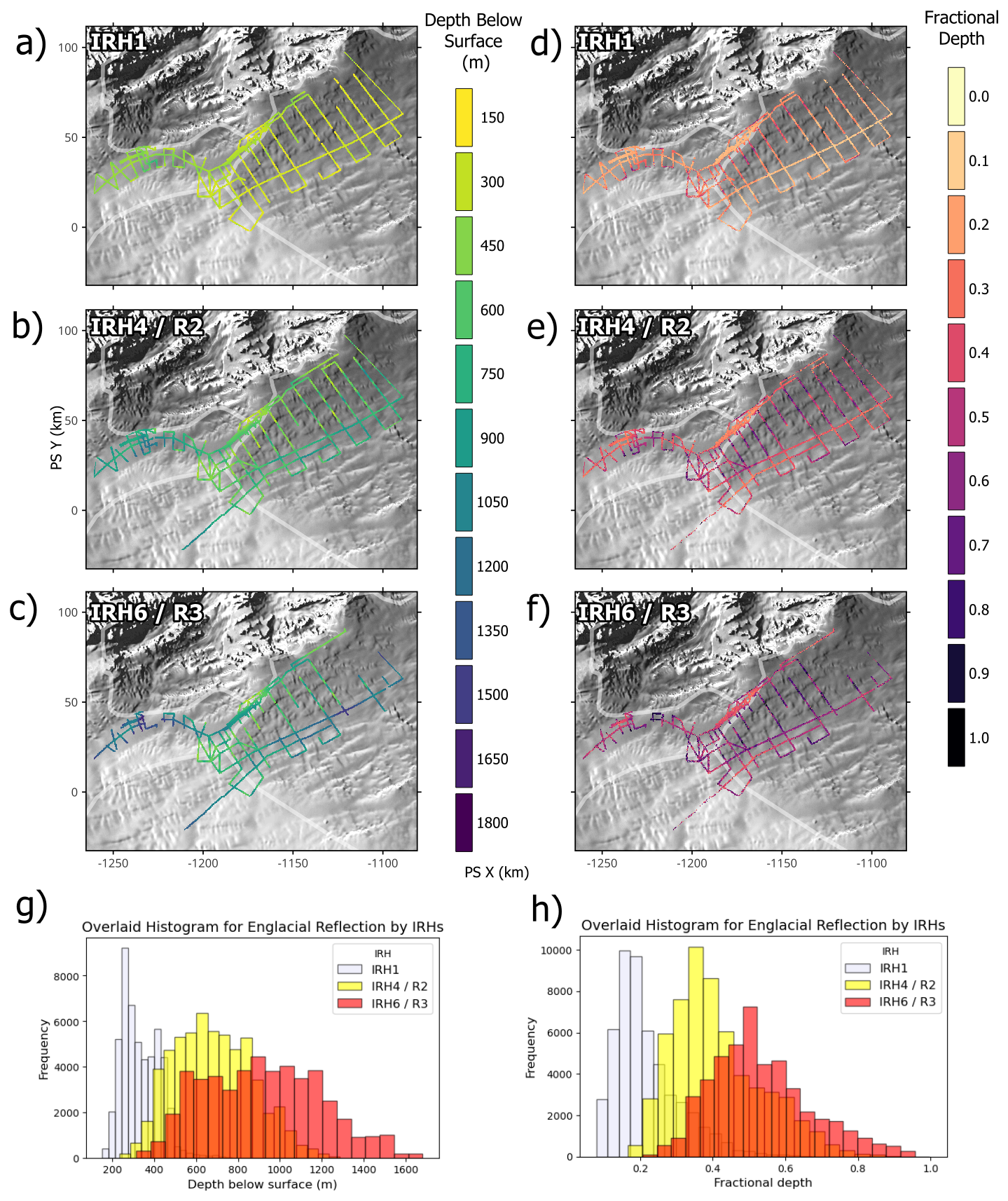
Figure 4 Internal Reflection Horizon (IRH) Depth Locations. Panels (a)–(c) display the absolute depth (in m) below the ice surface for three key englacial layers: the shallowest layer detected in this study (IRH1), and two additional layers, IRH4 and IR6, which are synchronised with ice-core chronology (corresponding to R2 and R3 in Bodart et al., 2021). Panels (d)–(f) illustrate the fractional depth of each layer (i.e., the ratio of its depth to the total ice thickness), where warmer colours indicate shallower positions and colder colours indicate deeper positions within the ice column. Panels (g)–(h) present the distribution of both the absolute depth below the surface and the fractional depth for these layers. In all panels, the Radarsat Antarctic Mapping Project (RAMP) topography is shown in the background, with thin white lines delineating the ice catchment boundaries (Mouginot et al., 2017). A comprehensive analysis of all englacial layers identified in this study is available in Appendix B: Figs. B1 and B2.

3.1.1 CECs Trough

In the CECs Trough (CT), most IRHs are laterally continuous and well preserved, although IRH7 becomes increasingly difficult to trace in the western sector (Fig. 5). The spacing between IRHs varies: IRH2 and IRH3 are closely spaced, whereas IRH3 and IRH4 are separated by a broader interval.

In the western part of the trough, near the boundary with the alpine terrain, multiple IRHs converge and merge into a thick, high-amplitude near-bed reflector. This pattern is consistently observed across several alpine valleys extending toward the Heritage Mountains and the head of Minnesota Glacier, where the geometry of the IRHs diverges from the underlying bed topography. Steep, fault-like structures locally truncate the stratigraphy and coincide with steep gradients in subglacial bed topography, and may reflect basal processes, deformation associated with local ice flow, or out-of-plane reflections.

Further upstream, towards the Institute Ice Stream (IIS) and above Subglacial Lake CECs (SLC), all reflections exhibit marked drawdown, particularly in the deeper IRHs (Fig. 6). Several internal reflections below IRH7 are strong and laterally continuous, even within the valley containing SLC (Rivera et al., 2015).

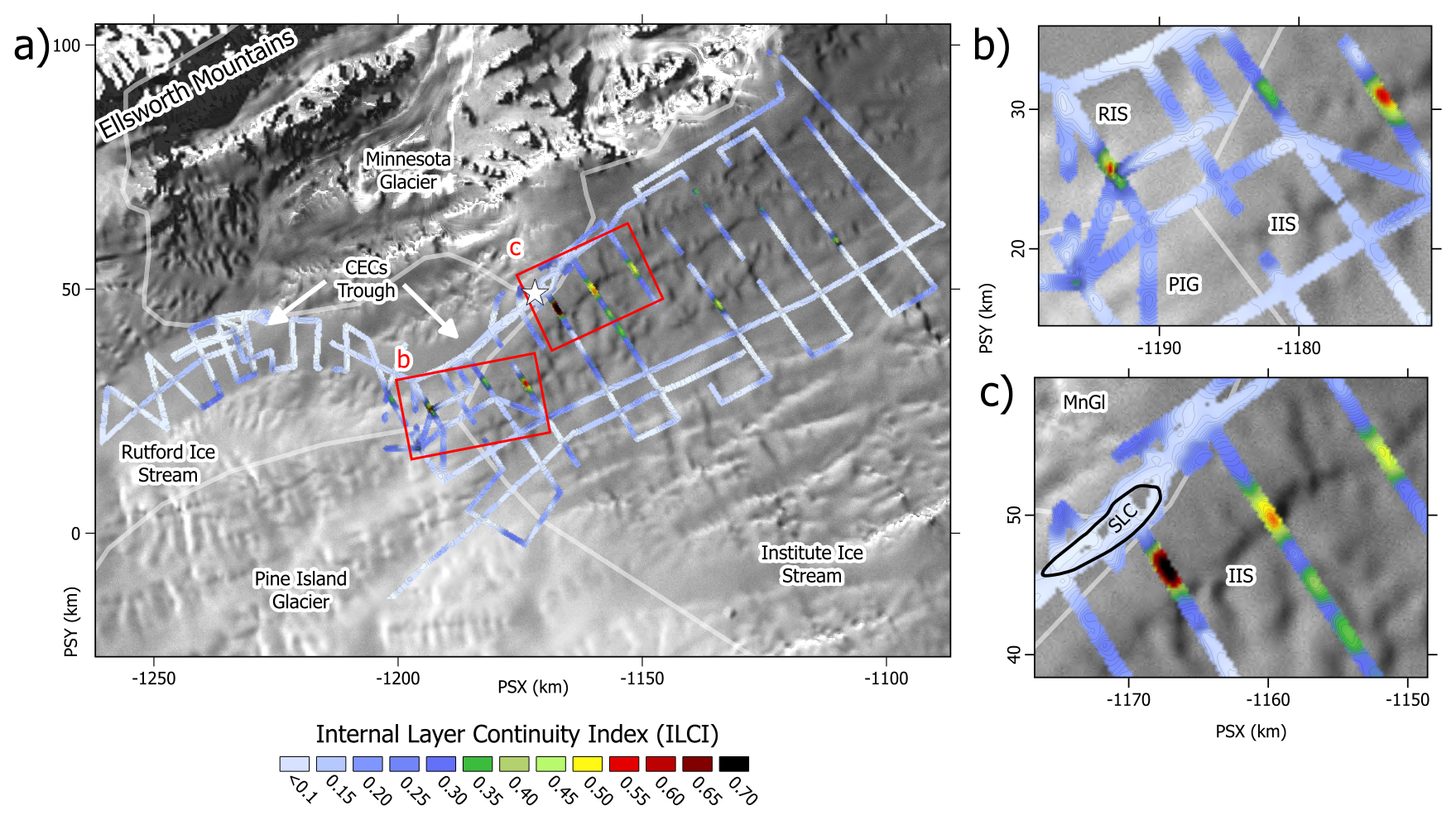
Figure 5 Internal Layer Continuity Index (ILCI) and englacial structure. (a) Internal Layer Continuity Index (ILCI) map across the Ellsworth Subglacial Highlands (ESH), with red squares showing the location of panels b and c, and white star highlighting the location of Subglacial Lake CECs (SLC). (b) Detailed view of the englacial structure continuity over the ice divide between Pine Island Glacier, and the Institute and Rutford Ice Streams. (c) Detailed view of the most laterally continuous englacial stratigraphy found across the subglacial highlands. Low ILCI values represent less laterally continuous Internal Reflection Horizons (IRHs), while higher values indicate more laterally continuous IRHs. It is notable that most of the well-preserved englacial stratigraphy is located near ice divides and over highs in the basal topography. In all panels, the Radarsat Antarctic Mapping Project (RAMP) topography is shown in the background, with thin white lines delineating the ice catchment boundaries (Mouginot et al., 2017).

3.1.2 Subglacial Highlands and Alpine Terrain

Across the subglacial highlands, IRHs are generally traceable but often become less distinct with depth. For example, IRH7 often becomes less distinctive as it approaches subglacial peaks, particularly along steep valley flanks (Fig. 7). The reasons for the lack of contrast are uncertain, but, for example, may relate to the incorporation and transport of basal material because the subwavelength distribution of debris is capable of causing backscattering that obscures the return relating to ice in the lower column (e.g., Winter et al., 2019; Franke et al., 2023). Even where stratigraphy is well preserved, interpretation is complicated by the spreading or merging of IRHs near topographic breaks.

The ice column in the highland regions is typically thinner and underlain by rugged bedrock topography, with narrow alpine valleys and steep-sided summits (Fig. 1c). In the lower part of the ice column, differences in radar reflections are observed within the meteoric ice, particularly in valley areas where internal reflections occur close to the ice–bed interface. In contrast, the interfluve areas, where the ice is thinner, are characterised by more diffuse reflections and an absence of internal layering in the lower ice (Fig. 7). Therefore, deeper layers could not be reliably picked due to changes in reflection properties and/or suboptimal radar system performance. While additional englacial layers may exist near the ice–bed interface, they may not be detectable because the radar system lacks the sensitivity required to resolve them at such depths.

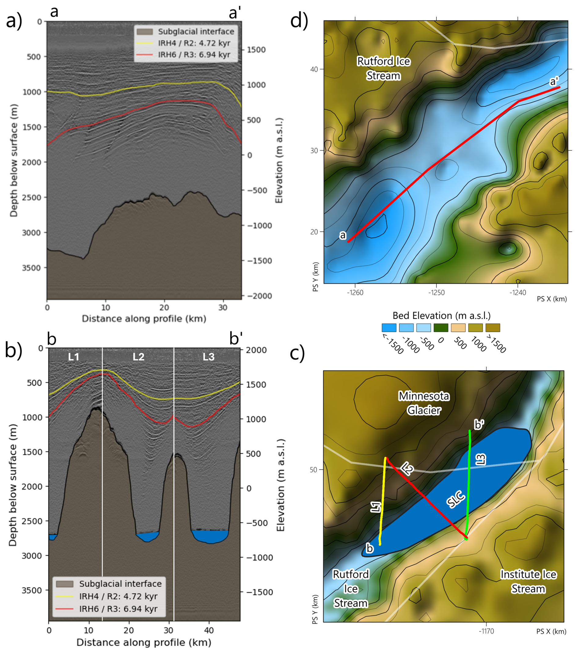
Figure 6 Internal Reflection Horizon (IRH) Continuity along CECs Trough and above Subglacial Lake CECs. Location of panel (a) in Fig. 3b (Area 1), and panel (b) in Fig. 3a (white star). (a) Example of steeply-dipping englacial reflections towards the end of the CECs Trough within the Rutford Ice Stream. The geometry of the IRHs could be indicative of basal melting above SLC. (b) Location of the RES profile shown in panel (a), also indicated in Fig. 1d. (c) Englacial geometry over Subglacial Lake CECs, displaying an evident drawdown of the englacial layers over SLC, and several continuous IRH below IRH6. The bathymetry of Subglacial Lake CECs is independently constrained from reflection seismic data (Brisbourne et al., 2023), providing a robust estimate of lake depth and sediment thickness beneath the ice. (d) RES survey geometry and acquisition setup for profiles shown in panels (c).

3.1.3 Ellsworth Trough

Most IRHs are well preserved and traceable, although IRH1 and IRH2 are poorly resolved near the ice divide due to low signal-to-noise ratio and signal saturation. Two principal topographic settings define the region: a deep trough, where IRHs show pronounced drawdown (particularly in deeper layers), and an adjacent alpine terrain separating the Ellsworth and CECs Troughs.

Lateral continuity of englacial reflectors varies across the study area. The lowest continuity was observed within the CECs Trough, particularly at the head of Minnesota Glacier, and along the Institute Ice Stream catchment (Fig. 5). In contrast, the highest continuity occurs across the subglacial highlands, where the stratigraphy is especially well preserved within narrow subglacial valleys (Fig. 5).

Low ILCI values suggest the IRH continuity is occasionally disrupted across the deep trough due to steep subglacial slopes (35–45° towards the Weddell Sea Embayment and 25–55° towards the Amundsen Sea Embayment), but the stratigraphy inferred from the current RES data suggest the ice column remains sufficiently coherent to trace most IRHs through the region. Near the divide, IRH1–3 remain closely spaced and maintain their configuration downstream, while IRH5–7 form a distinct group along the trough. IRH4 exhibits transitional geometry, aligning with the shallower group near the divide and the deeper group further downstream. In addition to low ILCI values, the ice column exhibits localised buckling and vertical discontinuities, particularly where tributary glaciers converge.

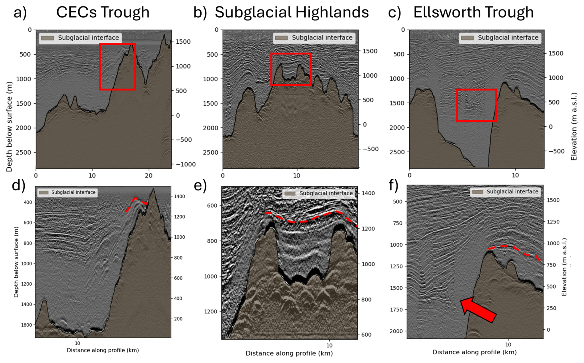
Figure 7 Examples of differences on internal reflectivity near the base of the ice in the Ellsworth Subglacial Highlands (locations of RES lines in Fig. 1d). (a) Southern end of the CECs Trough, and the boundary between englacial reflections near the mountain side (red dashed line in panel d). (b) Ellsworth Subglacial Highlands, and the boundary between englacial reflections over the interfluve and subglacial valley (red dashed line in panel e). (c) Ellsworth Trough, and the boundary between englacial reflections over the interfluve and subglacial valley (red dashed line in panel f). The red arrow in panel (f) indicate the changes in dipping angle of the englacial layer.

3.2 IRH uncertainties

Despite the fact that three RES systems were used to identify and map these IRHs, all of them have a similar central frequency of ∼ 150 MHz. Moreover, an empirical error analysis between all the CECs survey crossovers was performed and we obtained a maximum vertical difference of 17.6 m, but ∼ 99 % of the crossovers are below 15 m (Fig. B4). All of these error values are within the uncertainty range reported for each survey.

By comparing six intersections (1, 3, 4, 5, 7, 8 in Fig. 3b, c) between our IRH4 and R2 (described in Bodart et al., 2021) and two intersections (2 and 6 in Fig. 3c) with H2 (described in Ashmore et al., 2020), we estimated a mean vertical difference of approximately 15 m between IRH4 and R2, and 11 m between IRH4 and H2 – both within the expected uncertainty bounds of the respective radar systems. The same approach was applied to IRH6, comparing it with R3 and H3 across three intersections (points 3 and 5 for R3, and point 6 for H3 in Fig. 3). Maximum vertical differences were 17 m between IRH6 and R3, and 10 m between IRH6 and H3. Detailed values for each intersection are presented in Table 2.

We estimate a maximum vertical uncertainty of 5 m for ULUR-3.0 and 6 m for NG-CORDS for the deepest IRHs traced. Signal-to-noise ratios (SNRs) vary by system: 3.31–4.96 dB for NG-CORDS, 13.57–16.89 dB for ULUR-3.0 (January), and 13.83–16.71 dB for ULUR-3.0 (December). The estimated depth precision at the 68 % confidence level (Eq. 4) ranges from $\mathrm{\Delta }(r*)=\mathrm{1.99}$–2.43 m for NG-CORDS, 1.03–1.19 m for ULUR-3.0 (January), and 0.55–1.17 m for ULUR-3.0 (December). The total estimated vertical uncertainty for all IRHs is approximately ± 7 m (Table 2).

Table 2 Vertical differences (m b.i.s.) of intersections between CECs (Internal Reflection Horizon, IRH), BBAS (Rs), and IMAFI (Hs) surveys. Intersection points are shown in Fig. 3. Depth data for BBAS and IMAFI are from Bodart et al. (2021); Ashmore et al. (2020), respectively.

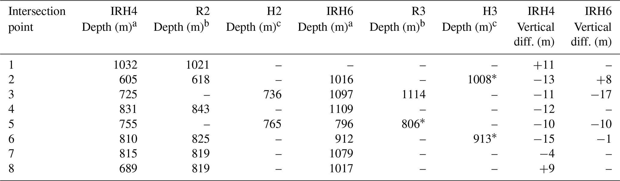
^a CECs uncertainty (± 7 m). ^b BBAS uncertainty (± 17 m). ^c IMAFI uncertainty (± 14 m). ^* From extension of R3/H3 to the intersection point.

3.3 Estimated and modelled ages for IRHs

Based on the match between IRH4 and R2 of Bodart et al. (2021), and applying Eq. (8), we assign an age of 4.72±0.284 kyr to IRH4. Similarly, using the reported age and associated uncertainty for R3 (Bodart et al., 2021), we assigned an age of 6.94±0.326 kyr for our IRH6.

To bracket the ages of IRHs lacking independent tie-points, we used a range of accumulation-rate estimates derived from snow stakes and regional modelling approaches. The contrasting “high” and “low” accumulation scenarios correspond to the upper and lower bounds of accumulation estimates from Noël et al. (2023), Arthern et al. (2006), and stake-derived rates (Sect. 1). These scenarios are relevant because, within the D–J framework, accumulation rate exerts a strong control on layer residence time and therefore has a first-order influence on the resulting age–depth structure, particularly at greater depth. Minimum ages were calculated using the highest accumulation rate applied at the IRH4 tie-point location (Fig. 4); and maximum ages were obtained using the lowest accumulation rates at the intersection (or closest stake), including Arthern et al. (2006) and Noël et al. (2023) (Table 1).

Across the seven IRHs, modelled ages range from approximately 1.23 (IRH1) to 7.19 kyr (IRH7) under the high-accumulation scenario, and from 1.8 to 17.6 kyr under the low-accumulation scenario (Table 3. See also Tables A1, A2, A3). These age envelopes indicate that the mapped IRHs span the Mid-Holocene, under a high accumulation scenario, and the full Holocene with the deepest layers potentially recording deglacial ice from the Late Pleistocene, under a low accumulation scenario.

Table 3 Synthesis of modelled ages (kyr) for each Internal Reflection Horizon (IRH) at intersection points across three study areas, derived using ranges of annual mean ice-equivalent accumulation rates, a, obtained from snow-stake measurements and modelling (Arthern et al., 2006; Noël et al., 2023). For each area, paired age values correspond to the lower and upper bounds obtained using a_min and a_max, respectively. Accumulation-rate ranges are: Area 1 (CECs Trough) a_max=0.318 and a_min=0.186 m ice-eq. yr⁻¹; Area 2 (Subglacial Highlands) a_max=0.253 and a_min=0.170 m ice-eq. yr⁻¹; Area 3 (Ellsworth Trough) a_max=0.268 and a_min=0.119 m ice-eq. yr⁻¹. Age ranges reflect a basal shear layer thickness of 20 %–30 %. Independent ages from the WAIS Divide ice core (Sigl et al., 2014) are included for comparison. For a full description of the age modelling using all available accumulation rates and basal shear layer thicknesses, see Tables A1, A2, and A3.

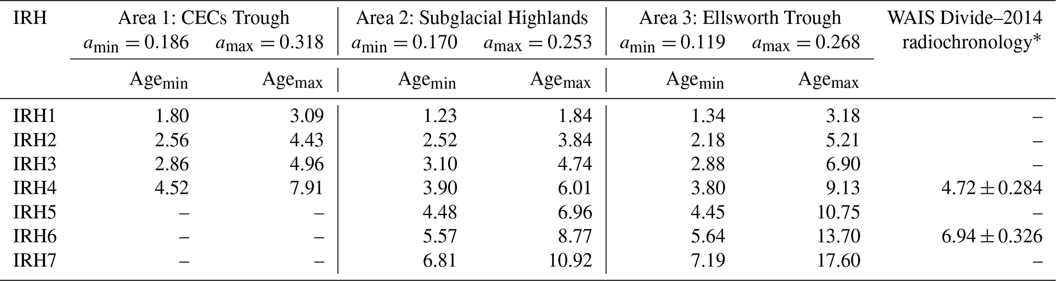
Notes: Age_min and Age_max denote the lower and upper bounds of modelled ages obtained using a_min and a_max, respectively. All accumulation rates are expressed as ice-equivalent depth rates. ^* Corrected using Eq. (8).

3.3.1 Quasi-Nye age estimates

The quasi-Nye age propagation at Site 2 yields age estimates that are consistent with the D–J age envelopes and preserve the same stratigraphic ordering and relative spacing of horizons. Using anchor depths of z₄=689.33 and z₆=857.27 m, quasi-Nye ages range from ∼ 5.48 (IRH5) to ∼ 8.74 kyr (IRH7). At this site, relaxing basal shear-layer assumptions primarily narrows the plausible age range for undated horizons without introducing systematic shifts that would alter our interpretations. In particular, quasi-Nye dating indicates that the deepest horizon (IRH7) is most consistent with an early- to mid-Holocene age, whereas substantially older ages arise only under the lowest-accumulation end-member scenarios within the D–J framework (see Fig. B3). Importantly, the choice of age-propagation method at Site 2 does not affect the principal conclusions regarding radiostratigraphic continuity, inferred ice-divide stability, or the spatial patterns of Holocene accumulation discussed in Sect. 4.1.

3.4 Millennial variability of surface accumulation

We used IRH ages derived from direct intersections with chronologically constrained IRHs from the WAIS Divide 2014 ice-core record to estimate accumulation rates in each of three Area of interest (Table 1 and Fig. 2).

We used snow stake data (Fig. 3) to estimate modern accumulation at intersection points in all three Areas of interest, and satellite-derived products to obtain average accumulation over the past 30 years (Table 1). By comparing these modern and satellite-derived estimates with englacial layer-derived accumulation rates modelled from reattaining the D–J model (i.e. R2–R3 and H2–H3, where available), we obtained a regional snapshot of Holocene accumulation across the three areas: the CECs Trough (Area 1), the Subglacial Highlands (Area 2), and the Ellsworth Trough (Area 3). It is worth noting that these regions exhibit slight differences in ice flow velocities: Area 1 is faster than Area 2 and Area 3, with typical surface velocities between 5 and 10 m yr⁻¹ (8 m yr⁻¹ at the intersection point), whilst Areas 2 and 3 generally remains below 5 m yr⁻¹ (4 m yr⁻¹ at the fastest intersection). In addition to surface velocity, ice advection, englacial layer displacement, and strain rates may also influence both modern and palaeo-accumulation patterns.

Rearranging the D–J model to solve for accumulation rate, and using the age of IRH4 constrained by R2 (from Bodart et al., 2021 ice chronology) at any given depth, we obtained accumulation estimates of 0.228 m ice-eq. yr⁻¹ in Area 1, 0.186 m ice-eq. yr⁻¹ in Area 2, and 0.169–0.186 m ice-eq. yr⁻¹ in Area 3 (Fig. 8). These values provide spatially resolved constraints on past accumulation across CECs Trough, Subglacial Highlands, and Ellsworth Trough. Spatially, accumulation has consistently been higher in the CECs Trough during both modern and Holocene periods, while the Subglacial Highlands show higher accumulation than the Ellsworth Trough during the Holocene, although this pattern appears to have reversed in recent decades. Temporally, accumulation rates derived from Arthern et al. (2006) are consistently higher across all regions, which may reflect the coarser spatial resolution and larger area of estimation associated with the satellite-derived dataset.

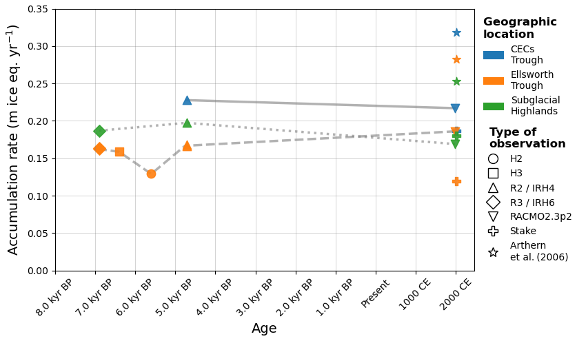
Figure 8 Surface accumulation rate variation since ∼ 7 kyr derived from the match of our Internal Reflection Horizon IRH4 and IRH6 to Bodart et al. (2021) R2 and R3, and Ashmore et al. (2020) H2 and H3 in Area 1 (cyan), Area 2 (red) and Area 3 in Fig. 3.

4 Discussion

4.1 Radiostratigraphy and chronology

Our study area encompasses an unusually complex subglacial landscape compared to other parts of West Antarctica (e.g., Ross et al., 2014; Karlsson et al., 2014; Rivera et al., 2015; Ashmore et al., 2020; Bodart et al., 2021) and East Antarctica (e.g., Sanderson et al., 2023; Franke et al., 2025). We traced seven internal reflection horizons (IRHs) exclusively across a region of rugged, high-relief topography, which we subdivide into three sectors: the CECs Trough, the subglacial highlands, and the Ellsworth Trough. Each sector presents distinct challenges for radiostratigraphic interpretation, including deep drawdown of IRHs in trough regions, shallow ice columns and contrasting basal reflectivity within the meteoric ice in the highlands, and disrupted stratigraphy caused by crevassing and converging ice flow (e.g., southern Institute Ice Stream and head of Minnesota Glacier). Despite these complications, the clear stratigraphic sequence allowed us to map IRHs continuously across areas with poor or disrupted internal layering, including fast-flowing ice, zones of transverse flow (e.g., near Minnesota Glacier), and alpine terrain.

In particular, the contrasts observed within the shallow ice over the southern end of CECs Trough and the alpine terrain (Fig. 7a and b) may indicate differences in physical properties, potentially linked to deposition during glacial or interglacial periods. Alternatively, the ice may be more compressed or contain elevated concentrations of volcanic ash. These variations warrant further investigation, as previous studies have suggested that basal ice with distinct properties may be widespread across West Antarctica (e.g., Winter et al., 2015, 2019).

IRH4 and IRH6 were confidently correlated with previously dated reflectors from the Pine Island Glacier (R2 and R3; Bodart et al., 2021) and Institute Ice Stream (H2 and H3; Ashmore et al., 2020) datasets. Although only two dated reflectors intersect our survey region, the matches are robust based on depth coincidence at crossover points and lateral continuity across the three areas. These correlations are supported by consistent reflector amplitude and stratigraphic positioning, particularly across distinct flow regimes. Using these dated IRHs, we rearranged the Dansgaard–Johnsen (D–J) model to calculate the accumulation rates responsible for their burial, which in turn allowed us to estimate the ages of our remaining unmatched IRHs across the region, ranging from 1.23–3.18 to 6.81–17.6 kyr for the shallowest and deeper IRHs, respectively. Within the D–J framework, accumulation rate exerts a first-order control on downward advection and vertical thinning. Lower prescribed accumulation results in slower descent of layers, longer residence times at a given depth, and consequently substantially older inferred ages relative to higher-accumulation scenarios. This effect becomes increasingly pronounced at depth, where vertical velocities diminish and the age–depth relationship becomes strongly non-linear. As a result, uncertainties in prescribed accumulation rate and basal shear-layer thickness accumulate over millennial timescales, amplifying curvature in the age–depth profile and increasing the sensitivity of the deepest englacial layers to small perturbations in model parameters. The quasi-Nye sensitivity test (Sect. 2.3.3) confirms that, over the depth interval bounded by the traced IRHs, the inferred age structure is robust to assumptions regarding basal shear-layer parameterisation. In contrast, the dominant source of remaining age uncertainty arises from variability in accumulation rates rather than from basal-condition choices. We note that the lower age range for the deepest IRHs would encompass the age of prominent West Antarctic reflector (Jacobel and Welch, 2005) which has an age of 17.4 ka, although here we cannot confirm it is the same layer. We note that this reflector is not as clearly expressed in the airborne IMAFI dataset (Ashmore et al., 2020), likely reflecting differences in radar system characteristics and acquisition geometry rather than its absence, and therefore avoid implying a direct one-to-one correlation.

Vertical offsets between matched reflectors across surveys range from approximately 10–17 m, which is within the expected resolution limits of the radar systems used (Table 2). These small discrepancies likely reflect a combination of radar-specific factors, including system resolution, acquisition timing, time-zero synchronisation, off-nadir scattering, and sparse 2D line geometry. Nonetheless, the consistent identification of IRH4 as the brightest reflection near R2 across multiple crossover points reinforces the reliability of these assignments.

Our stratigraphic correlations are further supported by published age estimates from Ashmore et al. (2020), dated H1 to 1.9–3.2 kyr, H2 to 3.5–6.0 kyr, and H3 to 4.6–8.1 kyr based on the Byrd ice-core chronology (Hammer et al., 1994). Together, these results establish a robust chronological framework for the Ellsworth Subglacial Highlands, enabling spatially resolved accumulation histories and supporting wider continental stratigraphic efforts.

4.2 Constraints on Divide-Proximal Ice-Flow Stability

The Internal Layer Continuity Index (ILCI) analysis supports the hypothesis of a stable ice divide (e.g., Denton et al., 1992; Bentley et al., 2010; Ross et al., 2011; Hein et al., 2016b; Small et al., 2025), indicating relatively undisturbed ice flow across the Subglacial Highlands and adjacent divide-proximal regions (Fig. 5). While ice flow within the main troughs appears broadly stable, the internal stratigraphy is locally disrupted by converging tributary glaciers from the Subglacial Highlands into CECs and Ellsworth Trough. This is particularly evident at the southern end of the Ellsworth Trough, where ice from the Subglacial Highlands and the alpine terrain to the west flows into the main trunk of the Institute Ice Stream. A similar pattern is observed in the CECs Trough near the head of Minnesota Glacier, where perpendicular inflow disrupts the internal layering, limiting the preservation of a coherent stratigraphy. These convergences result in low ILCI values probably because the ice becomes deformed as it accelerates and is channelled into narrower paths such as deep troughs or rift systems (e.g., Sanderson et al., 2023). This deformation, driven by shear, variations in basal conditions, and historical changes in flow (Bons et al., 2016), folds and disrupts the internal layers, reducing the consistency of radar reflections that the ILCI depends on. As such, low ILCI values suggest complex glacial dynamics and past or ongoing transitions in ice flow behaviour (Karlsson et al., 2012)

Although these local disruptions are notable, they do not contradict the broader inference of long-term ice divide stability across the region. Rather, they highlight the importance of high-resolution radiostratigraphic mapping for resolving spatial variability in internal structure that is not captured by continent-scale studies. Moreover, the complex flow patterns associated with rugged upland alpine topography may also influence the lateral continuity of englacial layers. Despite these local disruptions, our observations support the hypothesis that overall ice divide stability may coexist with dynamic flow reorganisation at outlet margins (suggested by the change in the dipping angle of IRHs in Fig. 7c), and that caution is warranted when extrapolating large-scale inferences to finer spatial scales.

Our findings are consistent with previous evidence that the inland Amundsen–Weddell divide has remained comparatively stable throughout the Holocene (e.g., Conway and Rasmussen, 2009; Bentley et al., 2010; Ross et al., 2011; Hein et al., 2016b; Siegert et al., 2019; Small et al., 2025). The expanded spatial coverage provided by our new radiostratigraphy allows this interpretation to be refined by identifying where regional stability coexists with localised dynamical complexity. Reduced ILCI values and deformation of deeper reflections along the Institute–Möller system and within the CECs and Ellsworth troughs (Figs. 5 and 7c) indicate enhanced strain and tributary interaction linked to complex basal topography, consistent with previous inferences of dynamically variable flow in these onset regions (e.g., Siegert et al., 2019; Ross et al., 2020). These low-continuity zones coincide with tributary convergence and topographic steering, where inflow into confined troughs promotes shear and reduced preservation of coherent stratigraphy. Importantly, this disturbance remains spatially restricted and does not extend far upstream toward the divide, where layering remains well preserved.

4.3 Accumulation History

Surface accumulation measured at snow stakes in Areas 1 and 3 (Fig. 1d; location of Areas 1–3 in Fig. 3) provides the primary observational constraint and is slightly lower than regional climate model estimates from RACMO2.3p2 (Table 1). At the CECs Trough (Area 1), stake measurements show an accumulation rate of 0.186 m ice-eq. yr⁻¹, compared to 0.217 m ice-eq. yr⁻¹ reported by Noël et al. (2023) for the northern sector. In the Ellsworth Trough (Area 3), stake-derived rates ranged from 0.119 to 0.168 m ice-eq. yr⁻¹, lower than the 0.186 m ice-eq. yr⁻¹ in RACMO2.3p2. Conversely, in the Subglacial Highlands (Area 2), measured accumulation rates (0.180–0.193 m ice-eq. yr⁻¹) slightly exceeded the RACMO2.3p2 estimate of 0.169 m ice-eq. yr⁻¹ (Fig. 8).

Stake measurements were consistently much lower than values derived from Arthern et al. (2006), which uses a coarser spatial resolution (5 km) compared to RACMO2.3p2 (2 km) and point-based stake data. This discrepancy likely reflects spatial averaging effects in coarse-resolution models, particularly in regions such as the Ellsworth Subglacial Highlands where accumulation rates vary over short distances. Empirical semivariograms of RACMO2.3p2 accumulation rates (Fig. B5) exhibit substantially smoother spatial variability, with semivariance increasing gradually over distances exceeding 40–50 km, indicating that the model under-represents short-wavelength accumulation variability captured by the stake observations. In contrast, snow-stake accumulation rates show that variability is concentrated at short length scales (Fig. B5), with semivariance increasing rapidly over lag distances of approximately 15–20 km before reaching a plateau. This corresponds to point-to-point accumulation differences of ∼ 0.03–0.04 m ice-eq. yr⁻¹, or roughly 15 %–25 % of the local mean accumulation rate.

Despite differences in magnitude, all datasets indicate a persistent spatial pattern: modern accumulation is highest in the CECs Trough area, intermediate across the Subglacial Highlands, and lowest in the Ellsworth Trough area (Fig. 8). This asymmetry highlights the spatial heterogeneity of surface mass balance across Ellsworth Land and appears to persist through time.

A comparison of in situ accumulation (modern accumulation rate) and the WAIS Divide 2014 ice-core chronology (past accumulation rate) reveals a reduction in surface accumulation since the deposition of IRH4 (∼ 4.92 kyr). In Area 1, using snow stake 087× and the corresponding RACMO2.3p2 value, we estimate a decrease of 18 %–25 % in accumulation since that time (Fig. 8). In Area 2, the reduction is estimated at 9 %–14 % (using stake 107), while Area 3 shows a wider range of 11 %–29 % (based on stake 105 and RACMO2.3p2 values; Table 1). These inferred reductions are consistent with previous evidence for elevated mid-Holocene accumulation relative to modern values across West Antarctica, derived from both internal radar reflectors and ice-core records. For example, enhanced mid-Holocene accumulation has been reported across parts of the Amundsen–Weddell–Ross Divide, followed by a late-Holocene transition toward lower modern rates in the WAIS Divide core record (Fudge et al., 2016; Bodart et al., 2023). Our spatially distributed estimates extend this pattern into the Ellsworth Subglacial Highlands and adjacent trough systems, suggesting that the reduction in accumulation since ∼ 5 kyr was regionally coherent rather than confined to isolated divide sites.

IRH6 dated to ∼ 6.9 kyr, provides an additional constraint on Holocene accumulation patterns. Using the same snow stakes and RACMO2.3p2 data, we estimated a reduction of 4 %–10 % in Area 2 since the deposition of IRH6. In Area 3, results vary depending on the reference dataset: a reduction of 4 % when using stake data, and a 13 % increase when using RACMO2.3p2 values. Nevertheless, accumulation rates for IRH6 show a consistent spatial gradient, with higher values in the CECs Trough area. This supports the interpretation that spatial heterogeneity in surface mass balance has remained relatively stable throughout the Holocene.

Our finding of a ∼ 13 %–29 % reduction in accumulation since ∼ 4.92 kyr, across the upper reaches of Pine Island Glacier, 18 %–25 % reduction in Rutford and 9 %–14 % in the Subglacial Highlands provide more spatial detail than previous studies and complement the ∼ 18 % mid-Holocene reduction reported by Bodart et al. (2021). Despite methodological differences and spatial scale, both studies indicate stable spatial accumulation patterns across the Amundsen–Weddell–Ross divide, supporting the robustness of our reconstructions and reinforcing the value of mid-Holocene climate forcing for regional ice-sheet modelling.

The apparent differences between our estimates and previous reconstructions (e.g., Bodart et al., 2021; Siegert and Payne, 2004) may be explained by a combination of spatial, chronological, and methodological factors. First, our analysis is based on snow stake observations from three spatially-localised areas, including two deep troughs; whereas both Bodart et al. (2021) and Siegert and Payne (2004) investigated much broader regions using airborne or satellite-derived internal reflection horizons (IRHs) and ice-flow modelling. This disparity in spatial scale is important, because local variability caused by topography, wind redistribution, or microclimatic effects may drive trends that are not representative of the wider ice sheet (e.g., Arcone et al., 2012; Dattler et al., 2019; Mills et al., 2019). Second, the local chronological approaches, specifically the time window, used may influence the understanding of the accumulation history. For example, we used IRH4 at ∼ 4.92 kyr as the reference horizon, while Bodart et al. (2021) dated their principal reflector to 4.72 ± 0.28 kyr. Siegert and Payne (2004) identified enhanced accumulation between ∼ 3.1–6.4 kyr and substantially lower values only prior to ∼ 6.4 kyr, suggesting that small offsets in horizon age and temporal resolution can alter whether the mid-Holocene is interpreted as a period of elevated or reduced accumulation relative to today. Third, the application of different methodologies further complicates direct comparison, potentially introducing offsets in how past and modern accumulation rates are defined. For example, our approach combines snow stake data with RACMO2.3p2 output, making the estimates sensitive to model biases, calibration intervals, and stake distribution. By contrast, Bodart et al. (2021) applied a one-dimensional ice-flow model to IRH-derived accumulation rates, comparing these against both RACMO2 output (1979–2019) and multi-century observational syntheses (1651–2010). Siegert and Payne (2004) employed RES stratigraphy constrained by the Byrd ice-core, offering a different form of temporal averaging. Fourth, elevation dependence provides an additional source of variation. In particular, Bodart et al. (2021) observed that sites below ∼ 1400 m often showed lower mid-Holocene accumulation relative to modern values, while higher-elevation sites recorded enhanced rates. Consistent with this, Siegert and Payne (2004), whose reconstructions focused on the central divide, found a mid-Holocene enhancement relative to present.

Finally, the temporal evolution of accumulation through the Holocene may reconcile the different perspectives. Both Bodart et al. (2021) and Siegert and Payne (2004) suggest that the mid-Holocene represented a relative maximum in accumulation, followed by a gradual decline towards modern conditions. Our results may therefore capture the latter part of this trajectory, emphasising the downward adjustment since ∼ 4.9 kyr, whereas earlier studies highlight the preceding peak. Rather than representing a fundamental contradiction, these findings may reflect complementary expressions of a broader transition from mid-Holocene high accumulation to present-day rates.

The RES surveys used in this study, as well as those by Siegert and Payne (2004), Bodart et al. (2021), and others, were not originally designed for the explicit purpose of investigating accumulation history. Given the complexity of accumulation patterns and the variability of survey strategies, there is a clear need for a systematic, purpose-designed campaign to investigate past accumulation across West Antarctica. Such an effort would benefit from a coordinated approach combining bespoke airborne and ground-based RES surveys with targeted ice coring, and complementary meteorological and geophysical observations.

5 Conclusions

1. Our analysis shows marked spatial variability in englacial layer geometry, reflecting the large range in ice thickness across the study area. Internal layers are deeper relative to ice thickness in the Ellsworth and CECs Troughs and comparatively shallower over the intervening subglacial highlands. This persistent contrast highlights the strong topographic control on englacial stratigraphy and underpins our subdivision of the region into three domains: the CECs Trough, the Subglacial Highlands and Alpine Terrain, and the Ellsworth Trough. These IRHs establish at least seven new radiostratigraphic tie points and represent a significant step toward strengthening the connection between the Weddell and Amundsen Sea Embayments.

2. We identified and traced seven internal reflection horizons (IRHs) across ∼ 2000 km of ground-based radar data, spanning ∼ 13 000 km² in the upper catchments of Pine Island Glacier (PIG), Rutford Ice Stream (RIS), and Institute Ice Stream (IIS). At least two horizons are directly tied to the WAIS Divide 2014 (WAISD-2014) ice-core chronology (IRH4 to 4.72 ± 0.238 kyr; IRH6 to 6.94 ± 0.326 kyr), providing robust age control and accumulation-rate estimates. For the remaining horizons, we applied the D–J age–depth model (Dansgaard and Johnsen, 1969) using accumulation rates derived from WAISD-2014 and in situ stake measurements. The modelled ages span from ∼ 6.81 to ∼ 17.5 kyr for the deepest reflector (IRH7), indicating that the traced stratigraphy records the Holocene and potentially extends into the Late Pleistocene.

3. The Internal Layer Continuity Index (ILCI) is generally very low along the subglacial trough, especially in areas where the ice surface velocity is relatively high and where different tributaries converge in the same trough, such as the southern end of Ellsworth trough or CECs trough at the head of Minnesota Glacier. However, the ice within alpine valleys across the subglacial highlands are very well preserved and the englacial stratigraphy is well preserved until the ice is deformed by ice flow over topography.

4. Modern and Holocene accumulation patterns derived from ice stake measurements, satellite observations, radiostratigraphy, and ice-core data indicate a persistent spatial asymmetry across the Amundsen–Weddell Ice Divide. Despite limited temporal coverage and high uncertainty in stake-derived accumulation rates, the broader spatial pattern agrees with satellite-based climatologies (e.g., RACMO2.3p2; Noël et al., 2023) and suggests that significant migration of the ice divide has not occurred since at least the mid-Holocene. This spatial stability supports recent findings from modelling and observational studies and has implications for long-term mass balance reconstructions across the central WAIS.

Overall, our study provides spatially resolved, age-constrained radiostratigraphy in a morphologically complex sector of West Antarctica, demonstrating that IRHs can be traced across diverse basal settings and flow regimes. By integrating multiple regional radiostratigraphies, we extend the spatial coverage of dated IRHs into a previously unresolved sector of the continent, directly contributing to the objectives of the AntArchitecture initiative (Bingham et al., 2025). Specifically, our findings support (1) the expansion of a continent-scale radiostratigraphic framework; (2) improved reconstructions of Holocene accumulation variability. In doing so, this work enhances our ability to constrain both past and future ice-sheet evolution across West Antarctica, and demonstrates that even in geologically complex terrain, coherent englacial stratigraphy can offer valuable constraints on the structure and dynamics of the Antarctic Ice Sheet through the late Quaternary.

Appendix A: Tables

Table A1 Accumulation rates for Internal Reflection Horizon (IRH) in Area 1 (CECs Trough) from Snow stake, Arthern et al. (2006), and Noël et al. (2023). Values are given for basal shear layer thickness, h, equal to 20 % and 30 % of the ice thickness. A dash (–) indicates no data.

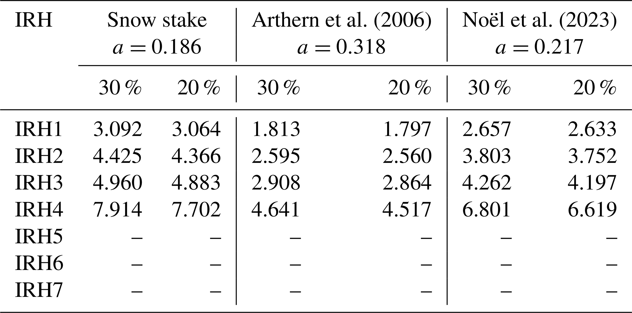
Table A2 Accumulation rates for Internal Reflection Horizon (IRH) in Area 2 (Subglacial Highlands) from Snow stake, Arthern et al. (2006), and Noël et al. (2023). Values are given for basal shear layer thickness, h, equal to 20 % and 30 % of the ice thickness.

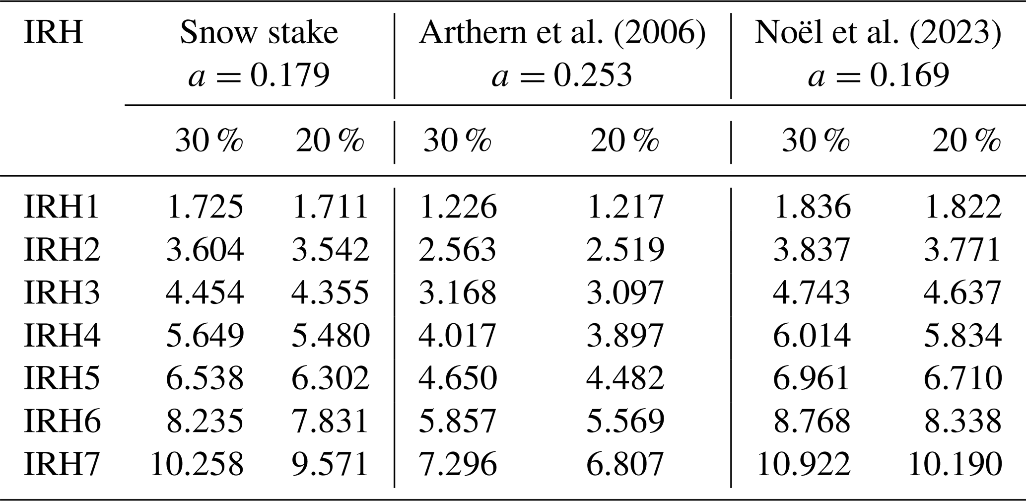
Table A3 Accumulation rates for IRHs in Area 3 (Ellsworth Trough) from Snow stake, Arthern et al. (2006), and Noël et al. (2023). Values are given for basal shear layer thickness, h, equal to 20 % and 30 % of the ice thickness.

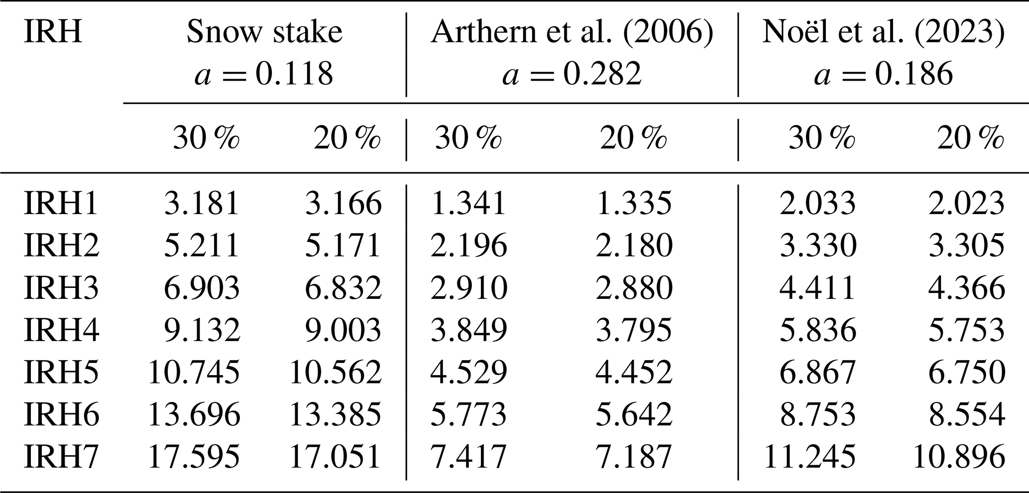
Table A4 Simplified quasi-Nye age estimates for internal reflection horizons (IRHs) at the modelling trace. Ages were calculated using observed IRH depths and anchored by the independently dated horizons IRH4 and IRH6. Following MacGregor et al. (2015), a constant effective vertical strain rate was assumed within the interval bounded by these dated horizons, and ages for undated IRHs were derived from the resulting non-linear quasi-Nye age-depth relationship.

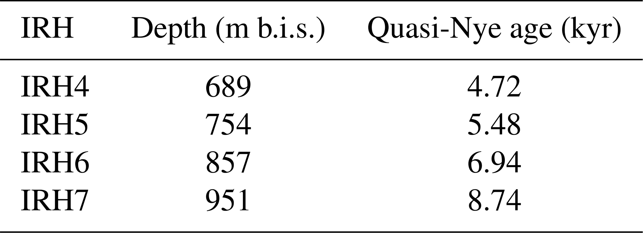
Table A5 Ice-penetrating radar systems used in this study and their principal technical characteristics.

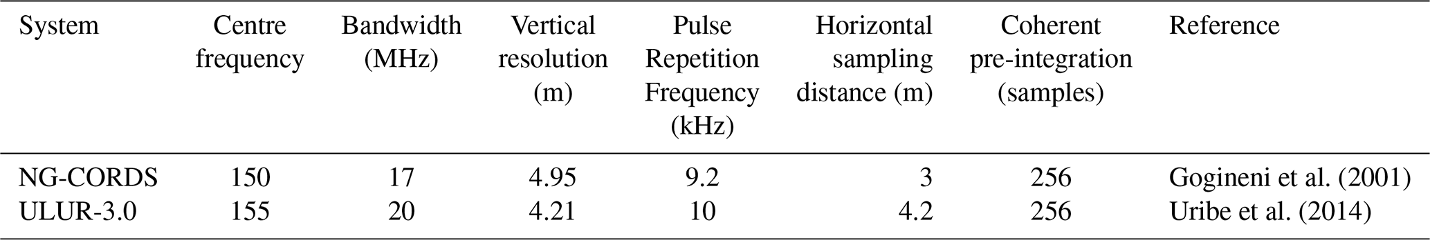
List of acronyms and abbreviations used in this study

Acronym	Definition
AWID	Amundsen–Weddell Ice Divide
BBAS	British Antarctic Survey Airborne Survey
CECs	Centro de Estudios Científicos
CT	CECs Trough
D–J	Dansgaard–Johnsen age–depth model
ET	Ellsworth Trough
ESH	Ellsworth Subglacial Highlands
H	Horizon (after Ashmore et al., 2020)
ILCI	Internal Layer Continuity Index
IMAFI	Institute–Minnesota Airborne Field Imaging
IRH(s)	Internal reflection Horizon(s)
IIS	Institute Ice Stream
LGM	Last Glacial Maximum
MnGl	Minnesota Glacier
NG-CORDS	Next-Generation Coherent Radar Depth Sounder
PASIN	Polarimetric Airborne Synthetic-aperture radar for Ice sounding and Navigation
PIG	Pine Island Glacier
R	Reflection (after Bodart et al., 2021)
RACMO2.3p2	Regional Atmospheric Climate Model, version 2.3p2
RES	Radio Echo Sounding
RIS	Rutford Ice Stream
RAMP	Radarsat Antarctic Mapping Project
SLC	Subglacial Lake CECs
ULUR-3.0	Ulloa-Uribe 3.0 RES system)
WAIS	West Antarctic Ice Sheet
WAISD-2014	WAIS Divide ice-core Chronology (2014 version)

Appendix B: Figures

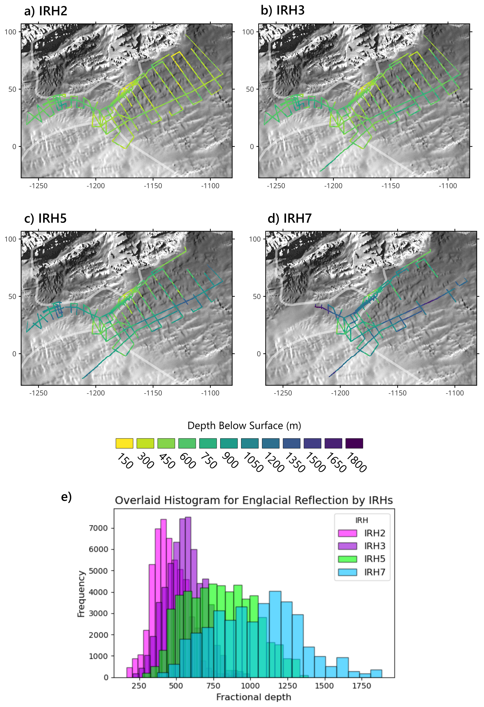
Figure B1 Spatial distribution and depth histograms of internal reflection horizons (IRHs). Panels (a)–(d) show mapped IRHs across the Ellsworth Subglacial Highlands, overlaid on Radarsat Antarctic Mapping Project (RAMP) topography. Thin white lines delineate the ice catchment boundaries (Mouginot et al., 2017). Each colour corresponds to depth below the ice surface, ranging from 150 m (yellow) to 1800 m (dark purple). (a) IRH2, (b) IRH3, (c) IRH5, and (d) IRH7. Panel (e) displays overlaid histograms of fractional depths for each IRH, illustrating their relative depth distributions. Shallower horizons (IRH2, IRH3) are concentrated between 250–700 m, while deeper horizons (IRH5, IRH7) extend to >1500 m.

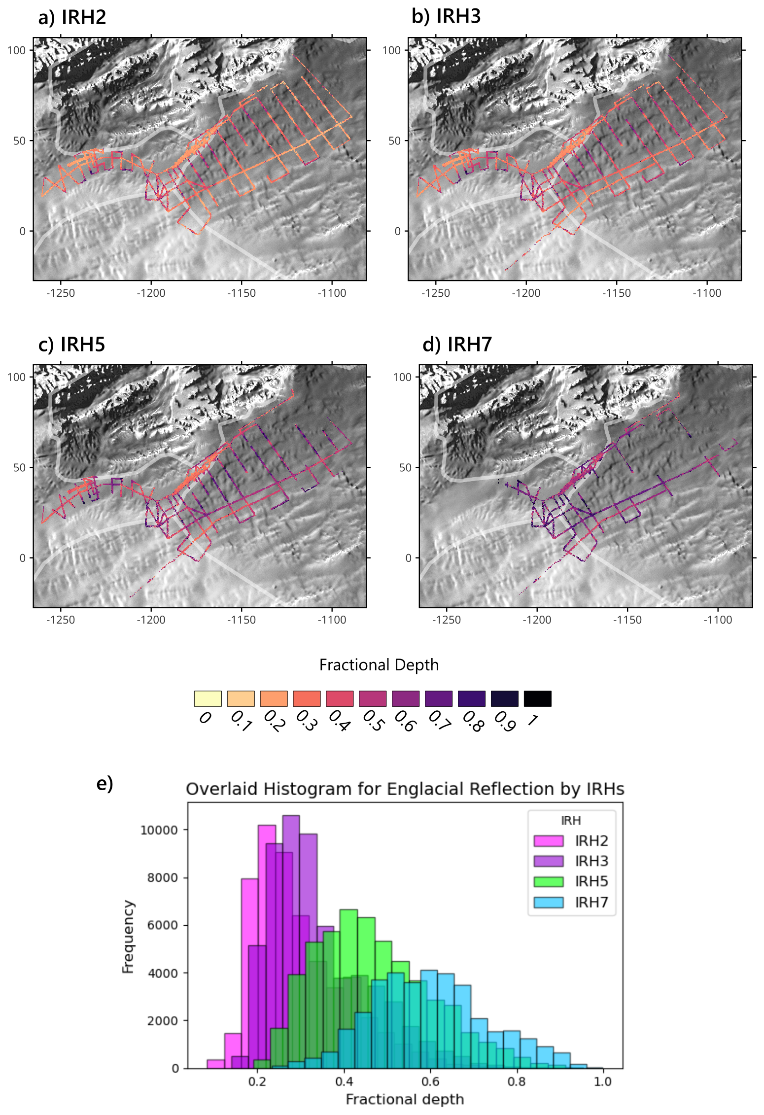
Figure B2 Spatial distribution and fractional depth histograms of internal reflection horizons (IRHs). Panels (a)–(d) show mapped IRHs across the Ellsworth Subglacial Highlands, overlaid on Radarsat Antarctic Mapping Project (RAMP) topography. Thin white lines delineate the ice catchment boundaries (Mouginot et al., 2017). Colours denote fractional depth within the ice column, ranging from 0 (surface; yellow) to 1 (bed; black). (a) IRH2, (b) IRH3, (c) IRH5, and (d) IRH7. Panel (e) presents overlaid histograms of fractional depths for each IRH. The shallower horizons (IRH2, IRH3) cluster at fractional depths of 0.15–0.35, whereas deeper horizons (IRH5, IRH7) extend more evenly through the ice column, with IRH7 reaching depths approaching the bed.

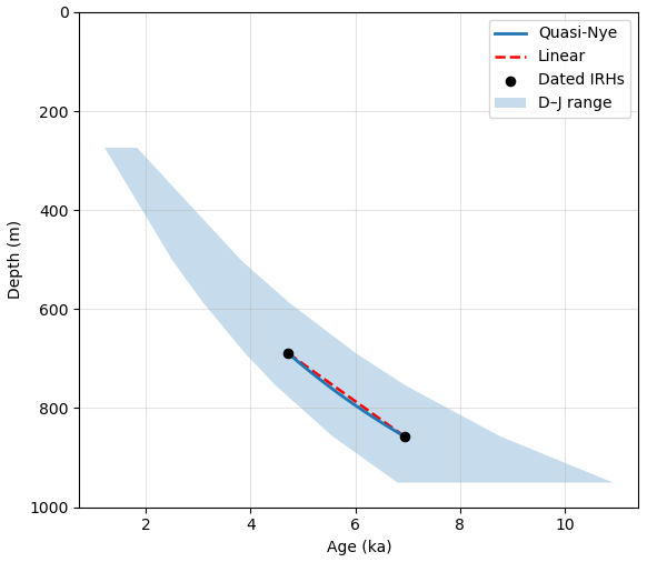
Figure B3 Comparison of age–depth relationships derived from different dating approaches. The shaded region represents the range of ages predicted by the Dansgaard–Johnsen (D–J) model using upper and lower bounds on accumulation rate. The solid blue line shows ages estimated using the quasi-Nye method (MacGregor et al., 2015). The dashed red line illustrates a simple linear interpolation between dated horizons. Black markers indicate independently dated internal reflecting horizons (IRHs) used as tie-points. The quasi-Nye solution closely follows the D–J envelope and deviates only slightly from linear interpolation over this depth interval, demonstrating that age estimates are largely insensitive to the choice of dating method within the range constrained by the available tie-points.

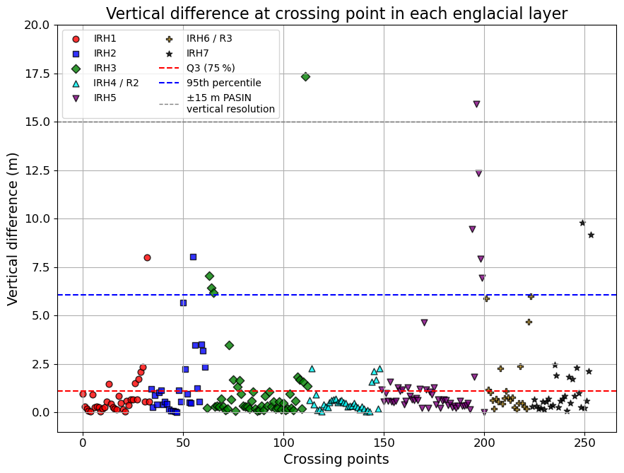
Figure B4 Vertical difference between crossovers of CECs Internal Reflection Horizon (IRH). Differences among IRH depth are presented for each IRHs in different colour and shape from the shallowest (IRH1) to the deepest one (IRH7). Additionally, we also marked the vertical resolution calculated for PASIN1 (Bodart et al., 2021) and key statistical percentiles.

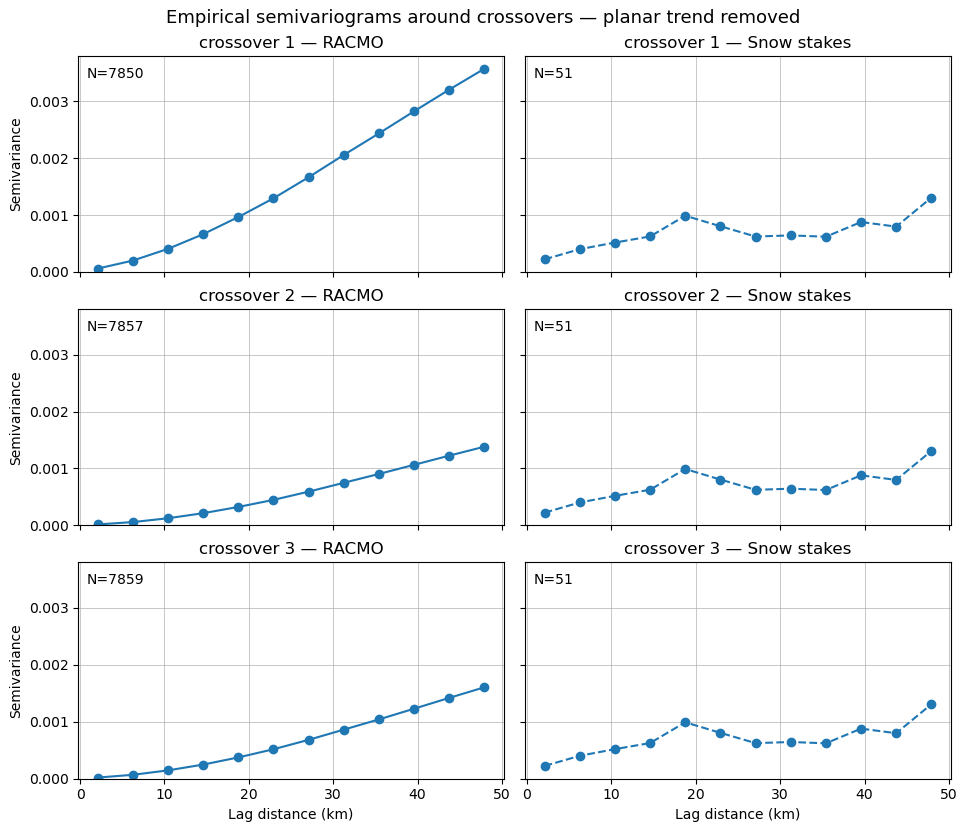
Figure B5 Empirical semivariograms of annual mean surface accumulation around three crossover locations, calculated after removal of a planar trend. Left panels show RACMO2.3p2 estimates and right panels show snow-stake measurements. Stake-derived accumulation exhibits stronger short-range variability (15–20 km), whereas RACMO2.3p2 displays smoother spatial structure over longer length scales. Numbers indicate the number of data pairs contributing to each semivariogram.

Appendix C: Firn air content sensitivity test

C1 Definition and interpretation of firn air content

Firn air content (FAC) is commonly reported in metres of air equivalent and represents the vertically integrated pore-space thickness within the firn column relative to pure ice density. Importantly, FAC does not represent a physical air layer of that thickness, but rather the thickness of air that would be obtained if all firn pore space were extracted and referenced to atmospheric pressure. FAC can be expressed as

$$\begin{array}{}\text{(C1)}& \mathrm{FAC}=\underset{\mathrm{0}}{\overset{z_f}{\int }}\left(\mathrm{1}-{\displaystyle \frac{\mathit{\rho }\left(z\right)}{{\mathit{\rho }}_{\mathrm{i}}}}\right)\mathrm{d}z,\end{array}$$

where ρ(z) is firn density, ρ_i is the density of ice, and z_f is the depth to pore close-off (or the effective firn column thickness represented by the model).

C2 Firn product and value selection

To evaluate whether spatial variability in firn properties could influence our depth conversion, we extracted FAC estimates from the NASA GSFC firn densification model (GSFC-FDM; Medley et al., 2022) over our three study sectors. GSFC-FDM provides temporally evolving firn properties across Antarctica; for our application, we used representative modern FAC values to quantify the impact on radar-derived ice-equivalent depths. Across our survey region, FAC varies between approximately 20 and 25 m (air equivalent).

C3 Propagation to ice-equivalent depth

A first-order way to incorporate FAC into depth conversion is to express IRH depth in ice-equivalent units by subtracting the air-equivalent pore-space contribution:

$$\begin{array}{}\text{(C2)}& z_{\text{ice-eq}}=z-\mathrm{FAC},\end{array}$$

where z is depth below the ice surface derived from radar processing and z_ice-eq is the corresponding ice-equivalent depth. At the representative modelling site (H=1433 m), FAC values of 20–25 m correspond to 1.4 %–1.7 % of the total ice thickness. Therefore, plausible spatial variability in FAC across the survey (ΔFAC∼ a few metres) modifies ice-equivalent depth by only ≲0.2 % of H.

C4 Implications for age estimates

The influence of a small depth perturbation on modelled age can be approximated locally as

$$\begin{array}{}\text{(C3)}& \mathrm{\Delta }t\approx {\displaystyle \frac{\partial t}{\partial z}}\mathrm{\Delta }z,\end{array}$$

where $\partial t/\partial z$ is the local age–depth gradient from the adopted age model (Dansgaard-Johnsen in the main analysis). Because FAC-driven depth adjustments are only a few metres, the resulting changes in inferred ages are small relative to the multi-millennial age range of the deeper IRHs. For example, using the IRH4–IRH6 anchors at Site 1 yields $\partial t/\partial z\approx \mathrm{0.013}\mathrm{kyr}{\mathrm{m}}^{-\mathrm{1}}$, such that a depth perturbation of Δz=3 m produces $\mathrm{\Delta }t\approx \mathrm{4}\times {\mathrm{10}}^{-\mathrm{2}}$ kyr (i.e., on the order of several tens of years). We therefore conclude that adopting a spatially variable FAC constitutes a methodological refinement but does not materially affect the age-depth structure or the interpretations presented in the main text.