Explicit representation of liquid water retention over bare ice using the SURFEX/ISBA-Crocus model: implications for mass balance at Mera glacier (Nepal)

In a warming climate, glaciers will experience increased liquid precipitation and melt, making it crucial to better understand and model the associated surface processes. This study presents a modeling approach developed to investigate the dynamic interaction between surface liquid water and bare ice using the SURFEX/ISBA-Crocus model. The implementation of the temporary retention of liquid water from rain or melt at the ice surface is described. The water is drained or can refreeze depending on meteorological conditions, directly affecting the albedo, thermal profile and glacier mass balance. This new development, tested to Mera Glacier (Nepal) shows an impact up to 6 % on the annual mass balance with contrasted effects depending on the meteorological conditions. During the pre-monsoon season, this implementation leads to greater mass loss (up to 20 %) due to surface liquid water, which enhances warming rather than compensating through refreezing. During the monsoon and post-monsoon seasons, it leads to less negative mass balance as a result of increased refreezing. Sensitivity analyses identified drainage and albedo as key model parameters. A 10 % change in stored liquid water drainage results in a 10 % change in annual mass balance. The albedo of bare ice and liquid water over ice represent the primary contributors to mass balance loss and the greatest uncertainties, making them priority targets for further investigation and improved characterization. This physically-based model development is essential for future climate projections worldwide, particularly given increasing melt, rainfall, and bare ice exposure under climate change.

1 Introduction

Mountain glaciers are significant contributors to global sea level rise and crucial water resources for millions of people in high-altitude regions (Immerzeel et al., 2020; Hock et al., 2019). They act as natural freshwater reservoirs, sustaining downstream populations and ecosystems, particularly in regions dependent on seasonal meltwater supplies (Pritchard, 2019). However, under ongoing climate change, mountain glaciers are experiencing accelerated mass loss worldwide (Zemp et al., 2019; The GlaMBIE Team et al., 2025), with projected mass losses of up to 41 % by 2100 globally (Rounce et al., 2023). Despite these global trends, regional responses exhibit substantial variability, highlighting key uncertainties in future glacier evolution (Brun et al., 2017).

Glacier mass balance, which directly controls glacier mass evolution, is primarily driven by the surface energy balance, where the interplay between atmospheric forcing and glacier surface conditions dictates ablation rates (Hock, 2005). Climate warming is not only increasing melt rates across most mountain glaciers but also raising the snow/rain transition (Łupikasza et al., 2019; Schauwecker et al., 2022; Fehlmann et al., 2018; Guo et al., 2021). These combined effects enhance the presence of liquid water on glacier surfaces, both through intensified melt and an increasing fraction of precipitation falling as rain. As the extent of bare ice exposure grows, understanding the complex interactions between liquid water and glacier surfaces becomes increasingly critical for accurate mass balance projections (Hartl et al., 2025; Réveillet et al., 2018).

The presence of supraglacial liquid water significantly influences both energy and mass balance through multiple mechanisms. Shortwave radiation absorption, the dominant driver of glacier ablation, is strongly modulated by surface albedo (Mölg and Hardy, 2004). The presence of liquid water has been shown to modify this balance, especially by reducing albedo, thereby increasing energy absorption and accelerating melt rates (Di Mauro et al., 2017; Di Mauro, 2020; Barandun et al., 2022; Gilardoni et al., 2022). Field observations in the Arctic indicate that liquid water presence can lower ice albedo by 20 %–70 % (Grenfell and Maykut, 1977), creating a strong positive feedback loop that enhances meltwater production (Tedstone et al., 2020; Hartl et al., 2020). Additionally, the refreezing of surface water at night releases latent heat, modifying the thermal structure of the glacier surface and influencing subsequent melt rates (Gilbert et al., 2014; Hartl et al., 2025). This diurnal melt-refreeze cycle can create thin layers of superimposed ice on the surface that exhibit a higher albedo (e.g. Volery et al., 2025).

Despite clear observational evidence of these processes, most current surface mass balance models do not explicitly represent the impacts of supraglacial liquid water (e.g., Mattea et al., 2021; Alexander et al., 2014). While some snow models incorporate water percolation schemes in the snowpack (e.g., Vionnet et al., 2012; D'Amboise et al., 2017), they generally do not account for the accumulation and impacts of liquid water on impermeable ice surfaces. Advanced hydrological models, such as those based on Richard's equations, have been applied to snowpack percolation (Wever et al., 2014), but few explicitly address supraglacial water storage. Existing models that consider water ponding are primarily developed for sea ice systems (Hunke et al., 2013; Popović and Abbot, 2017; Lüthje et al., 2006; Skyllingstad et al., 2015; Fettweis, 2007; Buzzard et al., 2018), highlighting a significant gap in glaciers surface energy and mass balance modeling. While studies acknowledge the importance of large supraglacial lakes in glaciers' energy and mass balances (Watson et al., 2016; Miles et al., 2018), the representation of small-scale water ponds and their diurnal cycle remains limited. Furthermore, existing energy balance models typically use static or simplified albedo parameterizations, neglecting its sensitivity to surface water cover (Hock, 2005; Gabbi et al., 2014).

In this study, we address these knowledge gaps by enhancing the SURFEX/ISBA-Crocus model to explicitly account for supraglacial liquid water storage and its feedback on bare ice surfaces. The development introduces a surface water reservoir that interacts with energy balance processes, modifying albedo and regulating mass balance through possible refreezing. The main aim of this study is to precisely describe the physical implementation of this reservoir and to discuss its sensitivity and the key parameters that need to be properly constrained in this development. To this end, the model was applied at a local point on a study site – Mera Glacier (Nepal) – to assess the significance of these processes in surface energy balance modeling. Mera Glacier was chosen to avoid relying on a virtual glacier and to take advantage of its well-documented climatic context and previous studies, as well as its exposure to strongly contrasting climatic regimes. By incorporating a more comprehensive treatment of surface water, this work aims to propose a physically-based model development that is transferable in both time and space, to improve glacier melt projections under present and future climate conditions.

2 Study site and data

2.1 Study site: Mera Glacier

Mera Glacier (Fig. 1) is a summer-type accumulation glacier located in the upper Dudh Koshi basin, in the Everest region (Central Himalaya, Nepal) and is monitored by the GLACIOCLIM program (https://glacioclim.osug.fr, last access: 18 December 2025) since 2007. Covering 4.84 km² in 2018, the glacier flows north, descending from 6390 to 4910 m a.s.l. with a flow divided into two branches at 5780 m a.s.l. (Mera branch and Naulek branch). More details on the characteristics of Mera Glacier are provided in Wagnon et al. (2013).

Mera Glacier gains most of its mass from June–September monsoon snowfalls driven by the South Asian monsoon (Wagnon et al., 2013; Thakuri et al., 2014; Pokhrel et al., 2024). This period, critical for understanding the glacier's climatic regime, is characterized by an average air temperature of 0.3 °C at 5360 m a.s.l. and 570 mm of precipitation at 4888 m a.s.l. (Khadka et al., 2022). The post-monsoon (October-November) is dry, sunny and windy, occasionally interrupted by typhoon-induced snowfall, while the winter (December-February) is colder but similarly dry and windy, with an average temperature of −10.4 °C. The pre-monsoon (March–May) is warmer and wetter, contributing about 25 % of the annual rainfall (Khadka et al., 2022).

2.2 Glaciological and meteorological data

Several Automatic Weather Stations (AWS), operated by the GLACIOCLIM observatory (https://glacioclim.osug.fr/, last access: 18 December 2025), are located at different altitudes, both on and off the glacier. In this study, we focus on one point in the ablation zone of the Naulek branch and use only the AWS located on the glacier at 5360 m a.s.l. (Fig. 1b), which records at half-hourly time step air temperature (T in K), relative humidity (RH in %), wind speed (u in m s⁻¹), incoming and outgoing longwave radiation (LW↓ and LW↑ in W m⁻², respectively), and shortwave radiation (SW↓ and SW↑ in W m⁻², respectively). Rainfall is monitored by a Geonor wind-shielded weighing bucket located in Khare (4888 m a.s.l.) (Fig. 1a), and the precipitation data are the same as in Khadka et al. (2024), i.e., there is no altitudinal gradient to correct for precipitation.

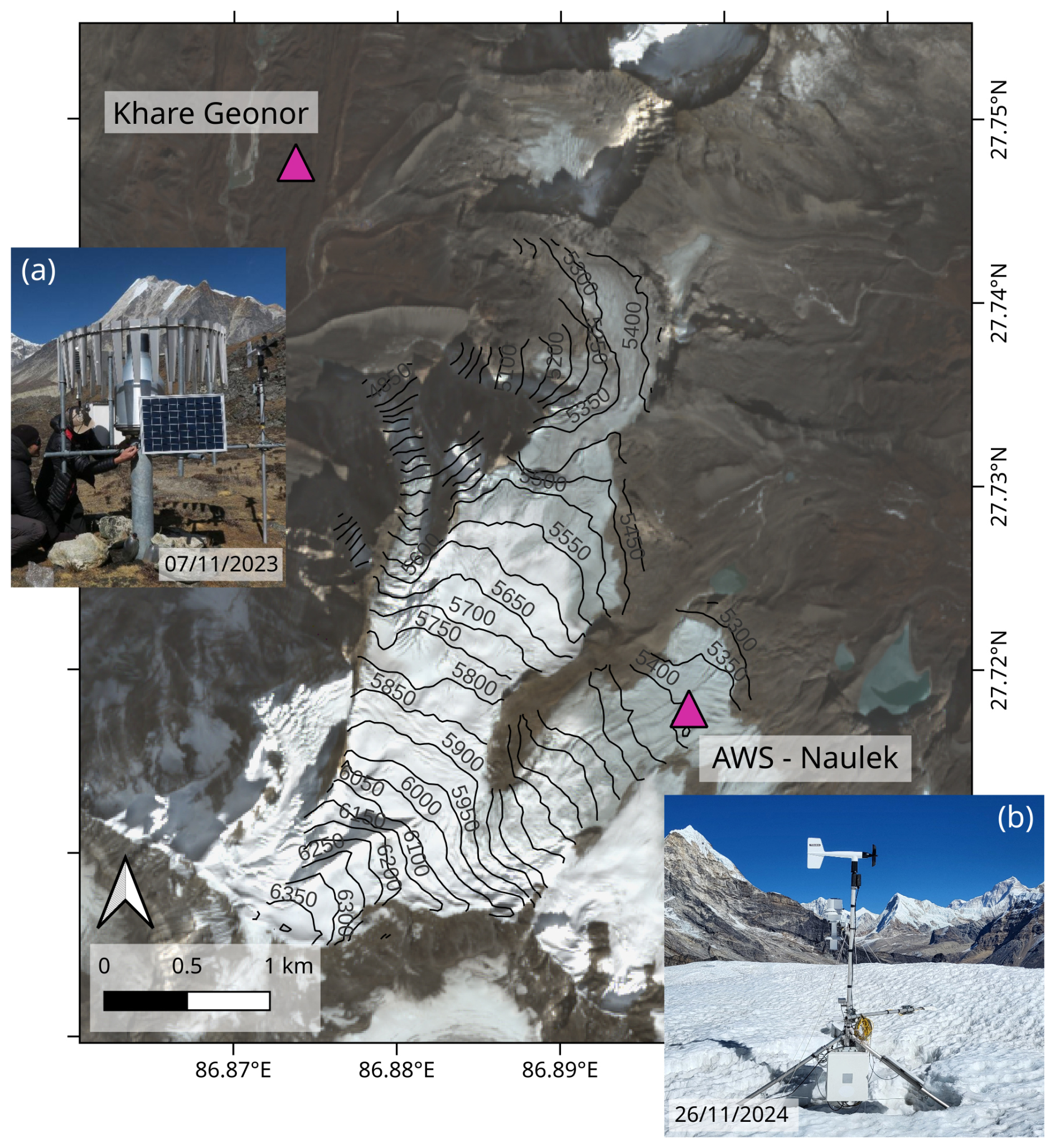
Figure 1 Map of Mera glacier (Nepal) showing the simulation point “AWS-Naulek” located on the Naulek branch (photo by Firmin Fontaine) and the Geonor at Khare (photo by Patrick Wagnon) which provides pluviometric data. The background image was acquired by Sentinel-2.

Gaps in the data occurred during the operational period (between November 2016 and 2022). The largest gap is almost a year long, from December 2017 to November 2018, in which case, as explained in Khadka et al. (2024), the gaps are filled by data from another AWS located at the same elevation less than two kilometers away using linear interpolation for some variables. In this study, we focus on years without long gaps (from November to November): 1 November 2016–1 November 2017, 1 November 2019–1 November 2020, 1 November 2020–1 November 2021, 1 November 2021–1 November 2022.

3 Methods

3.1 Crocus model description

3.1.1 Brief overview

Originally developed for seasonal snow cover in alpine environments, SURFEX/ISBA-Crocus (hereafter referred as Crocus, Lafaysse et al., 2025) is a physically based, model designed to simulate the microstructural evolution of snowpacks using a multilayer approach. Crocus is a one-dimensional column model and is used at the point scale. For spatial applications, the model is run at multiple independent grid points (i.e. without lateral transfers). In this study, the simulations are limited to a single-point configuration. The snowpack is discretized on a vertical grid, and using a Lagrangian approach, the model dynamically adjusts the vertical layering (number and size of layers, with a maximum of 50 layers) to represent changes in snowpack stratigraphy over time. Each layer represents snow with specific physical state variables, including mass, density, temperature, liquid water content, and microstructure properties (optical diameter and sphericity). The snowpack thermodynamical evolution is simulated by solving the energy and mass conservation equations at a 15 min time step (denoted as Δt in s). Key processes such as heat transfer, melting, sublimation, water percolation and refreezing are explicitly represented (Lafaysse et al., 2017).This computation of the liquid water and temperature fields in the snowpack is then used to simulate snow metamorphism, i.e. the evolution of the microstructural properties of snow.

Crocus has already been used to simulate glacier surface mass balance in the Alps (Gerbaux et al., 2005; Réveillet et al., 2018) and also in other mountainous regions such as the Andes (Lejeune et al., 2007) or the Himalayas (in a modified version that accounted for rock debris on ice: Lejeune et al., 2013; Giese et al., 2020). Crocus simulates glacier ice by treating it as a highly compacted, non-porous form of snow (e.g., Réveillet et al., 2018) with adjusted physical properties (such as the albedo, aerodynamical roughness length, or thermal conductivity). In this configuration, layers are classified as ice when their density exceeds 850 kg m⁻³, a threshold that can be adjusted if needed. Pure ice has a maximum density of 917 kg m⁻³.

Crocus requires atmospheric forcing variables including air temperature, relative and specific humidity, wind speed and direction, incoming shortwave and longwave radiation, and precipitation (solid and liquid). These inputs are used at an hourly resolution in the model, and an interpolation is realized for all atmospheric variables except for rainfall and snowfall where a mean rate is applied. Additionally, we assume no geothermal heat flux at the base of the snowpack (ground flux set to zero), thus excluding any basal melt contribution. We use the Crocus version within the SURFEX plateform (Masson et al., 2013).

3.1.2 Crocus limitations for water percolation over ice

In Crocus, liquid water percolation follows a conceptual bucket model (Lafaysse et al., 2017), where each layer retains water up to a defined threshold. This threshold, known as the liquid water holding capacity, is expressed as a percentage of the layer’s pore space. Layers act as stacked reservoirs that fill up until reaching this limit, which depends on their porosity. The excess water then drains into the underlying layer. By default, the maximum water holding capacity is set to 5 % of a layer’s pore space (Vionnet et al., 2012), consistently with the experiments from Coléou and Lesaffre (1998) on snow.

However, the standard implementation of Crocus was not designed to properly handle the presence of non-porous and impermeable layers such as ice. Indeed, up-to-now these layers were treated as having zero holding capacity but remained permeable. Consequently, liquid water is allowed to pass through pure ice, without any retention or barrier to percolation. Specifically, it means that in the case of a temperate ice column, all liquid water percolates without any storage or refreezing, causing all rain and meltwater to convert directly to runoff without surface retention. Conversely, if the ice column temperature falls below the triple point (273.15 K), refreezing can occur within sufficiently cold layers during percolation. Consequently, potential water retention mechanisms observed on glaciers, such as ponding, refreezing, or temporary storage of liquid water within surface irregularities, cannot be represented in the Crocus current version.

3.2 Implementation of surface liquid water retention over bare ice surfaces

The implementation of surface liquid water retention on ice surfaces is inspired by observations showing that glacier surfaces, due to their rugosity, can temporarily accumulate liquid water in small surface irregularities (Fig. 2). To model this water retention, we based our approach on the developments in SISVAT, the snow-ice scheme of the regional climate model MAR (Modèle Atmosphérique Régional, (Fettweis, 2007)), as described in (Lefebre et al., 2003).

3.2.1 Buffer description

Surface water retention is modeled using a virtual surface layer called a buffer, that holds liquid water between time steps, representing water accumulated in surface ice rugosity (Fig. 2). This buffer explicitly accounts for liquid water at the surface only, without representing percolation into or water storage within the underlying ice layers. The buffer is implemented as a scalar variable rather than as an additional physical layer in the model structure. This choice avoids unnecessary complexity in the definition and treatment of layers within the model routines, while still capturing the key processes associated with surface water storage. The model workflow, which provides information on the state of routine modifications and their order of use, can be found in the Supplement, Sect. S1.

The buffer layer is implemented as an optional parameterization within Crocus that can be activated or deactivated through model configuration. When activated, it allows explicit consideration of the thermal influence of liquid water on the underlying ice, its effects on surface albedo, and its contribution to the surface mass balance. This implementation introduces a feedback between the surface energy balance and the thermal profile of the underlying layers at each time step. When deactivated, the model runs in its basic configuration.

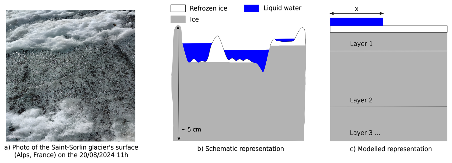
Figure 2 Photo of an observed pond of liquid water in the rugosity of the surface of Saint-Sorlin glacier (Alps, France) with schematic and modeled representations of the phenomenon on a cross-sectional view of the glacier.

The buffer exists only when the three following conditions are met: (i) the entire column is ice (i.e. density greater than 850 kg m⁻³) ; (ii) there is no snowfall during the time step and (iii) no freezing rain. Otherwise the buffer is completely drained to the runoff and the model reverts to its default configuration with no surface water storage. These conditions are necessary to avoid overly complex situations such as snowfall accumulating on a surface already covered by stored liquid water. Although such events do occur in reality, the treatment of these specific cases is beyond the scope of this study.

The mass of the buffer is updated at each time step, accounting for rain and melted ice added to it, any refreezing, and the rate of decay. The mass balance equation for the buffer is given by:

$$\begin{array}{}\text{(1)}& {\displaystyle \frac{\partial M_{\mathrm{buff}}}{\partial t}}=R_{\mathrm{melt}}+R_{\mathrm{rain}}-R_{\mathrm{refrz}}-{\displaystyle \frac{M_{\mathrm{buff}}}{{\mathit{\tau }}_{\mathrm{D}}}}\end{array}$$

where M_buff(t) (in kg m⁻²) is the mass of liquid water in the buffer, R_melt, R_rain and R_refrz (in kg m⁻² s⁻¹) are the rates of melt, rain and refreezing respectively and τ_D is the characteristic time of drainage linked to the so-called drainage coefficient D by Eq. (2).

$$\begin{array}{}\text{(2)}& D=\exp \left({\displaystyle \frac{-\mathrm{\Delta }t}{{\mathit{\tau }}_{\mathrm{D}}}}\right)\end{array}$$

A maximum threshold, z_max,buff (in m), is set for the buffer to prevent unrealistic water storage. Once the water content in M_buff exceeds this threshold, any additional meltwater or rainfall is transferred directly to the runoff variable exiting the glacier without further interaction with the ice surface. By default, z_max,buff is set to 1 cm but can be adjusted by the user. On the other end, when M_buff equals zero, the buffer's thermal and radiative effects are deactivated by setting the fraction parameter x to zero (see Sect. 3.2.2 for details on the energetic impact), while the mass remains in the buffer.

At the end of each time step, the drainage coefficient D is applied to M_buff to partially empty the buffer, mimicking the natural downward flow of water on a glacier. As for the excess water storage, the drained water goes directly to the runoff. This gradual drainage occurs as long as water is present in the buffer, even without additional water from melt or rainfall, ensuring that the buffer empties over multiple time steps. D is an empirical variable fixed by the user, ranging from 0 (complete drainage at each time step) to 1 (no drainage) and is arbitrarily set to 0.995. The impact of this choice will be tested and discussed in Sect. 5.2.2. Note that D is linked to τ_D via Δt, the time step duration (in s), to ensure the simulation remains independent of the chosen time step.

3.2.2 Impact of liquid water on ice thermal profile

For the rest of this section, variables are expressed as v⁺ or v⁻, where + and − denote the variable (v for the example) before and after the process described in the subsection.

The top layer's thermal profile is adjusted to account for the presence of water. In the model, the heat diffusion equation is solved to determine the column thermal profile. When liquid water is present at the ice surface, an additional term $K_{\mathrm{buff}}^{+}$ (in W m⁻²) is included to the heat diffusion equation to account for the conductive fluxes between the liquid water (with a fixed temperature of 273.15 K (Hunke et al., 2013)) and the top layer of ice.

$$\begin{array}{}\text{(3)}& K_{\mathrm{buff}}^{+}=\mathrm{2}x{\mathit{\lambda }}_b{\displaystyle \frac{T_{\mathrm{0}}-T_{\mathrm{1}}^{+}}{\mathrm{\Delta }z}}\end{array}$$

where x is the fraction of a representative surface area of the grid point which is impacted by the buffer (i.e. the fraction of ice covered by water on Fig. 2c), λ_b the thermal conductivity of liquid water (in W m⁻¹ K⁻¹), $T_{\mathrm{1}}^{+}$ the temperature (in K) of the top of the first layer, T₀ the temperature of the buffer which is at the triple point (273.15 K) and Δz the thickness of the first layer (in m). λ_b is fixed at 0.6 W m⁻¹ K⁻¹, an empirical value recommended by McLaughlin (1964) for water at 273.15 K.

The fraction x was introduced to modulate the buffer's influence on the thermal profile and albedo, since water only covers part of the surface. When the buffer scheme is activated and liquid water is present (M_buff>0 kg m⁻²), x is set by the user to a constant value in the range $x\in ]\mathrm{0},\mathrm{1}]$. This user-defined value represents the fraction of the representative surface area affected by the buffer and must be greater than zero to ensure that the buffer's thermal contribution is integrated into the heat diffusion equation's conduction term and its radiative effects are included in albedo calculations. When the buffer scheme is deactivated (either through model configuration or when buffer conditions are not met) or when M_buff equals 0, x is effectively set to zero in the calculations, decoupling any thermal and radiative effects. In this study, x is set by default to 0.2 when the buffer is active, a value chosen to allow significant thermal contribution while keeping ice as the dominant surface component. This choice and its impact are discussed in Sect. 5.2.1.

The heat equation for the first layer, using a formalism adapted from Boone and Etchevers (2001), with the additional conductive term is:

$$\begin{array}{}\text{(4)}& c_{\mathrm{I}}{\mathit{\rho }}_{\mathrm{1}}{z}_{\mathrm{1}}{\displaystyle \frac{T_{\mathrm{1}}^{+}-T_{\mathrm{1}}^{-}}{\mathrm{\Delta }t}}=G_{\mathrm{0}}^{+}-G_{\mathrm{1}}^{+}+R_{\mathrm{0}}-R_{\mathrm{1}}+K_{\mathrm{buff}}^{+}\end{array}$$

where $G_{\mathrm{1}}^{+}$ (in W m⁻²) is the heat flux between layers 1 and 2. c_I (2106 J kg⁻¹ K⁻¹) is the ice specific heat capacity, ρ₁ (in kg m⁻³) and z₁ (in m) are respectively the volumic mass and the thickness of layer 1. $T_{\mathrm{1}}^{+}$ and $T_{\mathrm{1}}^{-}$ (in K) are temperatures for layer 1. R₀ and R₁ are the radiative fluxes (in W m⁻²) entering and passing through the layer, respectively. The heat flux between the atmosphere and the surface, G₀, is the sum of all the energy fluxes at the surface:

$$\begin{array}{}\text{(5)}& G_{\mathrm{0}}=\mathit{ϵ}({\mathrm{LW}}^{\downarrow }-\mathit{\sigma }{T}_{\mathrm{1}}^{\mathrm{4}})-H-LE+{\mathcal{P}}_{\mathrm{r}}{c}_{\mathrm{W}}\mathrm{\Delta }t(T_{\mathrm{a}}-T_{\mathrm{0}})\end{array}$$

where ϵLW^↓ (in W m⁻²) is the incoming longwave radiation, $\mathit{ϵ}\mathit{\sigma }{T}_{\mathrm{1}}^{\mathrm{4}}$ (in W m⁻²) is the emitted longwave radiation expressed with Stefan-Boltzmann law and 𝒫_rc_WΔt(T_a−T₀) (in W m⁻²) is the energy carried by the liquid precipitations with 𝒫_r (in kg m⁻² s⁻¹) the rainfall flux, c_W the liquid water specific heat capacity (4218 J kg⁻¹ K⁻¹), T_a (in K) is air temperature.

Note that over the ice, the radiative components of Eq. (5) are calculated without considering liquid water and the turbulent fluxes remain unchanged. This choice is made based on the assumption that the exchange between the atmosphere and the surface primarily occurs with ice, since water covers only a small fraction of the surface (x=0.2). As mentioned above, it is assumed that liquid water on the ice only affects the ice by conduction. In addition, albedo parameters are set accounting for the presence of liquid water at the surface (see Sect. 3.2.5).

3.2.3 Melt

When the heat diffusion equation provides a temperature $T_i^{+}$ above T₀, melting occurs. The amount of melted mass, M_melt,i, is limited either by the available energy (related to $T_i^{+}$) or by the solid mass present in the layer before melting, denoted as M_s,i (in J m⁻²):

$$\begin{array}{}\text{(6)}& M_{\mathrm{melt},i}=min\left(c_{\mathrm{I}}{\mathit{\rho }}_i\right(T_i^{+}-T_{\mathrm{0}});M_{\mathrm{s},i})\end{array}$$

Equation (6) is evaluated for all layers to determine if a layer melts completely within a time step. If multiple layers are melting, multiple iterations are performed.

In our implementation, the melt calculation (Eq. 6) remains unchanged, but the fate of the melted mass M_melt,i is modified as M_melt,i is stored in M_buff. Meltwater from all layers in the ice column is accumulated in this buffer, regardless of depth. As melting is confined to the uppermost layers (typically the first few centimeters in our simulations) due to the absence of basal flux and attenuation of penetrating shortwave radiation, this approach avoids the need to define an arbitrary depth threshold in the code.

Then, the total mass of layer i is defined after melting (including both solid and liquid fractions) as M_i (in J m⁻²). After melting, the depth and total density are updated based on the change in solid mass:

$$\begin{array}{}\text{(7)}& {\displaystyle }{z}_i^{+}=z_i^{-}{\displaystyle \frac{M_{\mathrm{s},i}-M_{\mathrm{melt},i}}{M_{\mathrm{s},i}}}\text{(8)}& {\displaystyle }{\mathit{\rho }}_i^{+}={\displaystyle \frac{M_i-M_{\mathrm{melt}}}{z_i^{+}}}\end{array}$$

ρ_i accounts for both the solid and liquid fractions of the layer. In contrast, the model also defines a “dry density”, denoted as ρ_dry,i (kg m⁻³), which represents only the solid fraction. As the melt is stored within the buffer outside the layering system, it is considered in the total density calculation which includes the liquid fraction.

Finally, the layer temperature, T_i, is updated to account for the cooling effect of the phase change:

$$\begin{array}{}\text{(9)}& T_i^{+}=T_i^{-}-{\displaystyle \frac{M_{\mathrm{melt}}}{c_{\mathrm{I}}{\mathit{\rho }}_{\mathrm{dry},i}{z}_i^{-}}}\end{array}$$

3.2.4 Refreezing of the surface water

Refreezing depends on the availability of stored liquid water in the buffer and the energy deficit of the first layer. The refrozen mass, M_refrz (in J m⁻²) is expressed in Eq. (10):

$$\begin{array}{}\text{(10)}& M_{\mathrm{refrz}}=min(K_{\mathrm{buff}}^{+}\mathrm{\Delta }t,M_{\mathrm{buff}}{L}_m)\end{array}$$

where L_m is the latent heat of ice fusion (3.337 × 10⁵ J kg⁻¹).

A positive $K_{\mathrm{buff}}^{+}$ indicates that heat is conducted from the buffer to the first layer, meaning the first layer is sufficiently cold and/or the buffer is thin enough for a phase change to occur. If the energy deficit in the first layer exceeds the available liquid water, the excess energy is redirected to the first ice layer. This ensures that any heat not used for refreezing in the buffer contributes to cooling the ice column, thereby affecting the energy state of the glacier surface layer. The temperature of the first layer is then updated as follows:

$$\begin{array}{}\text{(11)}& T_{\mathrm{1}}^{+}=T_{\mathrm{1}}^{-}-{\displaystyle \frac{min(\mathrm{0},K_{\mathrm{buff}}^{+}\mathrm{\Delta }t-M_{\mathrm{refrz}})}{c_{\mathrm{I}}{\mathit{\rho }}_i{z}_i}}\end{array}$$

When refreezing occurs, the liquid water in the buffer is converted to refrozen ice. This process increases the surface mass of the glacier, directly impacting its mass balance, and alters energy exchanges.

The model determines whether to create a new surface layer or aggregate the refrozen mass with the existing surface layer. If the refrozen mass M_refrz is thick enough (greater than $\mathrm{1}/\mathrm{10}$ of the first layer thickness), a new refrozen ice layer is created at temperature T₀ with a density of 917 kg m⁻³. Otherwise, M_refrz is aggregated into the existing surface layer at its temperature.

To track the proportion of refrozen ice within the upper layers and properly compute albedo, a refreezing fraction variable r_frac,i is introduced for layers $i\in [\mathrm{1},\mathrm{2}]$. This variable ranges between 0 (bare ice) and 1 (fully refrozen ice) and is calculated differently depending on the refreezing scenario: when a new layer is created, the new surface layer receives r_frac,1 = 1, while when refrozen mass is aggregated with an existing layer, r_frac,1 is calculated as a weighted average based on the relative thicknesses of the refrozen and existing ice. The variable r_frac,i remains stored between time steps, allowing the albedo calculation to account for the presence of refrozen ice in the surface layers. When melting occurs in layer i, r_frac,i is reset to 0, assuming the refrozen layer melts first.

A detailed description of the layer management strategy, numerical thresholds, and the mathematical formulation of r_frac,i can be found in the Supplement, Sect. S3.

3.2.5 Albedo

In the default version of Crocus, ice surface albedo is handled by dividing incoming solar radiation into three distinct spectral bands ([0.3–0.8], [0.8–1.5], and [1.5–2.8] µm), with a constant albedo value prescribed for each band. The spectral albedo is used to attenuate incoming radiation in each band, and the remaining energy penetrates into the ice and is gradually absorbed, following an exponential decay with depth. Originally, ice albedo in Crocus was treated as a fixed value, independent of depth or surface conditions. However, the model architecture allows for albedo computation across the top two layers of the surface. Building on this, the present study introduces a modified scheme that enables the prescription of distinct albedo values for each of these layers, depending on surface conditions (bare ice, refrozen ice, or ice with liquid water). In this modified configuration, albedo is computed based on the properties of the first two layers, allowing for a more realistic representation of varying ice surface states.

The albedo calculation is updated to also consider the presence of liquid water and refreezing ice. When surface liquid water is present (as indicated by a non-zero M_buff), the first layer albedo follows Eq. (12).

$$\begin{array}{}\text{(12)}& {\mathit{\alpha }}_{\mathrm{1}}=x{\mathit{\alpha }}_{\mathrm{wat}}+(\mathrm{1}-x)(r_{\mathrm{frac},i}{\mathit{\alpha }}_{\mathrm{refrz}}+(\mathrm{1}-r_{\mathrm{frac},i}\left){\mathit{\alpha }}_{\mathrm{ice}}\right)\end{array}$$

where $i\in [\mathrm{1},\mathrm{2}]$ refers to layers 1 or 2. Without liquid water, the first layer's albedo is determined using Eq. (13). The albedo of the second layer, meanwhile, always follows Eq. (13).

$$\begin{array}{}\text{(13)}& {\mathit{\alpha }}_i=r_{\mathrm{frac},i}{\mathit{\alpha }}_{\mathrm{refrz}}+(\mathrm{1}-r_{\mathrm{frac},i}){\mathit{\alpha }}_{\mathrm{ice}}\end{array}$$

For snow-covered surfaces, the classic albedo parameterization is maintained, with values dependent on optical diameters and layer age (Vionnet et al., 2012).

Due to the lack of observational albedo data for liquid water over ice surfaces and for superimposed ice on mountain glaciers, as well as the potentially high spatial variability, no fixed values can be prescribed. As a result, the choice of albedo values is fully user-defined. The specific albedo values adopted in this study are presented in Sect. 3.3. Given the critical influence of albedo on energy balance, sensitivity tests are conducted (Sect. 4.3.3), and this aspect is further discussed in Sect. 5.2.4.

3.3 Simulation settings

3.3.1 Simulation description

Crocus was run at a point scale, at the AWS located on the ablation area of Mera Glacier, for the years 2016–2017, 2019–2020, 2020–2021 and 2021–2022. Model runs with a 15 min temporal resolution, using default parameters and scheme processes as presented in (Lafaysse et al., 2017). Simulations ran from 1 November to 1 November each year and used two distinct configurations: an unmodified base version (R18 as described in Réveillet et al., 2018) and our updated version incorporating buffer implementation (BV). A 60 m column of temperate ice (7 layers at 273.15 K) with a density of 917 kg m⁻³ was used as initial conditions. In order to illustrate the diurnal cycle of the buffer, results are presented at first over four days (from 1 to 5 April 2022), during which bare ice is exposed. Then, other periods are considered for the impact at annual scale.

3.3.2 Model calibration and evaluation

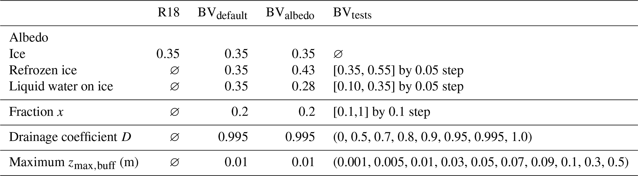
The parameter values used for all simulations are summarized in Table 1. The ice albedo value is set based on available observations and is consistent with the findings of Khadka et al. (2024) (Fig. S2 in the Supplement). However, due to the lack of observational albedo data for the specific surfaces, two sets of simulations are performed. In the first setup (simulation named BV_default), a fixed albedo value was applied to all three surface states: bare ice, refrozen ice, and liquid water over ice. This approach was chosen to limit their differentiated impact in order to better explore the effect of the other parameters (Sect. 4.3). In the second setup (simulation BV_albedo), distinct albedo values were prescribed for each surface type, and analysed over the 2021–2022 period. Values have been chosen in agreement with literature. Supraglacial water reduces the albedo by about −20 % (e.g., Grenfell and Maykut, 1977), and thus the albedo of liquid water over ice is decreased to 0.28 in the model. On the contrary, superimposed ice generally leads to an increase in albedo and is set to 0.43 (i.e. an increase of 23 %, following Traversa and Di Mauro, 2024). The other variables have been arbitrarily chosen and sensitivity tests are performed as described in the following section.

The default simulation (BV_default) is compared to observations (see Fig. S3 and Table S1 in the Supplement). While some biases are observed in simulated mass balance, the surface temperature at the AWS shows very good agreement with observations, with a mean bias of 0.34 °C without systematic bias. In particular, the model accurately captures the timing of temperate ice conditions, which is critical for assessing surface energy processes. All details regarding model calibration and evaluation, including a thorough discussion of their implications for this study, are provided in the Supplement, Sect. S2.

3.3.3 Sensitivity tests

To assess parameter sensitivity (Sect. 4.3), tests were conducted on fraction x, drainage coefficient, maximum buffer thickness, and surface state albedo (see Table 1) for the 2021–2022 period. Note that fraction x excludes 0, as the presence of a buffer without any impact on the thermal profile is not physically meaningful. The drainage coefficient was tested across its full range, with a finer resolution between 0.9 and 1 to better capture its influence on water retention and drainage. The sensitivity to the maximum buffer thickness was explored up to 50 cm to define the limits of the model's applicability. Albedo of liquid water over ice varies up to 70 % following Grenfell and Maykut (1977) and albedo of the refrozen ice up to 60 %, to explore a broad range of possible surface conditions, accounting for the high uncertainty in these values.

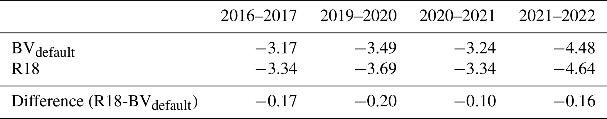
Table 1 Parameters used for the different simulations: base version (R18), buffer version with fixed albedo (BV_default), buffer version with specific albedo for the surface (BV_albedo) and for sensitivity tests.

4 Results

4.1 Buffer dynamics

In order to illustrate the diurnal cycle of the buffer, results are presented over four days (from 1 to 5 April 2022), during which bare ice is exposed (Fig. 3).

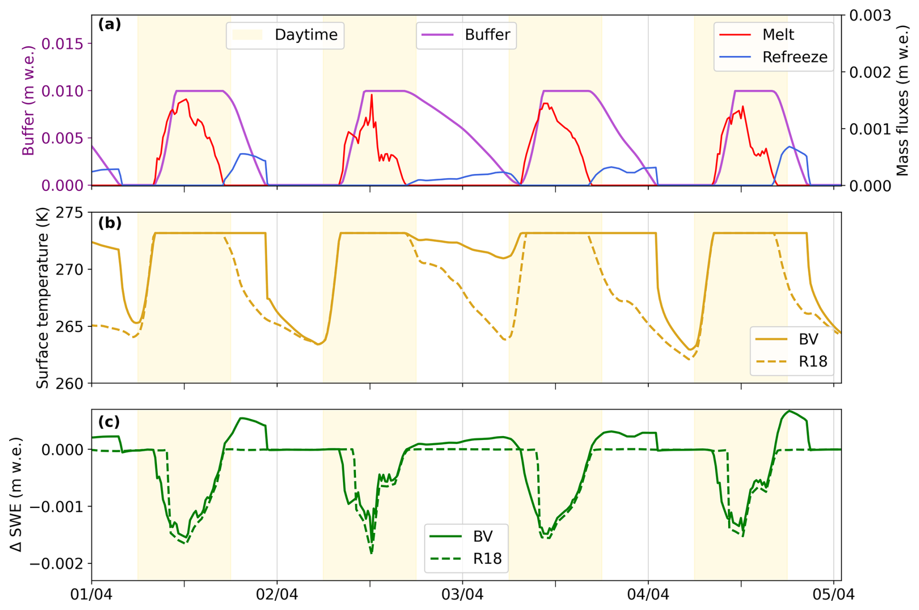
Figure 3 (a) Evolution of the buffer in purple, melt and refreeze fluxes in red and blue, (b) surface temperature (in yellow) and (c) Delta SWE evolution (in green) for the BV_default version in thick line and R18 in dashed line, from 1st to 5 April 2022, Mera Glacier 5360 m a.s.l.. Yellow shaded areas indicate daytime (6 a.m. to 6 p.m.). Vertical gridlines mark midnight, with minor ticks at noon.

During the day, atmospheric conditions are favorable for surface melt, leading to the storage of liquid water in the buffer until it reaches its maximum capacity of 0.01 m w.e. (Fig. 3a), beyond which any additional melt contributes to runoff (not shown). Then, during the night, the atmospheric conditions lead to surface cooling (surface temperature < 0 °C, Fig. 3b), causes stored water to refreeze, delaying surface cooling in BV_default compared to R18. In this example, the refreezing represents between 10 % and 40 % of the daily melt volume during the period (Fig. 3a). Then, the buffer gradually empties as stored water simultaneously refreezes, forming new ice layers at the surface, and drains according to the coefficient D, with drainage being either complete (Fig. 3a) or partial (see Fig. 6c or e), depending on meteorological conditions.

The buffer implementation has a significant impact on the glacier mass balance due to the water storage capacity that allows surface refreezing. Both versions show a decreasing ΔSWE (the difference in mass balance from one time step to the next) during melting periods, but BV_default shows increases of 0.1 to 0.5 mm w.e. (i.e. an increase in SWE of about 10 mm w.e. during 8 h of the night) during refreezing periods (Fig. 3c). In contrast, R18 shows negligible temporal ΔSWE variation ($<{\mathrm{10}}^{-\mathrm{3}}$ m w.e.) during the night.

The duration of nighttime refreezing shows significant temporal variability over the study period. Typically lasting 6–9 h (Fig. 3c), the refreezing process can extend from as little as 2 h to as long as 10 h in other periods. This variability primarily depends on water availability in the buffer at sunset and subsequent nighttime cooling rates.

BV_default initiates ΔSWE decreasing 1–2 h earlier in the day compared to R18 (Fig. 3c), not due to earlier melt onset, but because of fundamental differences in refreezing temporality. R18 immediately refreezes the first 1–2 h of melt production deeper in the ice column, while the ice remains cold from winter conditions. Conversely, BV_default retains this water at the surface, where it refreezes during the night. This creates a fundamentally different refreezing temporality, with the buffer acting as a temporary reservoir, delaying refreezing by an average of 8 h.

The maximum buffer threshold of 0.01 m w.e. regulates both immediate runoff and subsequent refreezing cycles. When daytime melt intensity reaches this threshold (typically around 10 a.m., Fig. 3a), it triggers immediate runoff and limits water availability for nighttime refreezing.

4.2 Consequences on energy and mass fluxes in different meteorological contexts

4.2.1 Impact at annual scale

When comparing the mass balance simulated with BV_default and with R18, at the AWS of Mera Glacier over the four studied years (Fig. 4) we find that, on average, incorporating the buffer leads to a less negative annual mass balance, with a mean difference of 0.16 m w.e., corresponding to approximately 4 % of the annual mass balance. This impact varies by year, ranging from 0.1 m w.e. (3 %) to 0.20 m w.e. (6 %) of the annual mass balance (see Table 2). If the albedo of liquid water over ice and refrozen ice are different from the albedo of the ice, the BV_albedo version will not lead to a significant difference (less than 1 %, see Fig. S4 in the Supplement S4). Sensitivity tests will provide further explanation in Sect. 4.3.3.

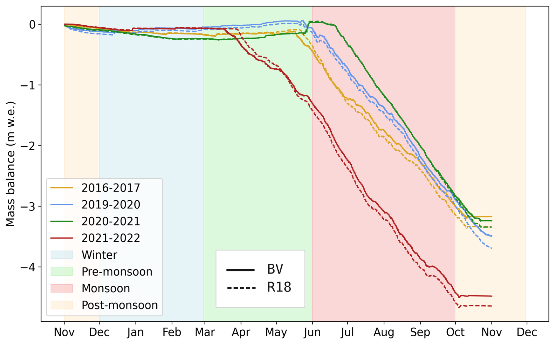
Figure 4 Simulated seasonal mass balance evolution (in m w.e.) for different hydrological years (2016–2017, 2019–2020, 2020–2021, and 2021–2022). Solid and dashed lines represent the two versions (BV_default and R18 respectively). Background colors indicate different seasons: winter (blue), pre-monsoon (green), monsoon (red), and post-monsoon (orange).

Table 2 Simulated mass balance for different years in m w.e.

The influence of the buffer implementation on mass balance exhibits strong seasonal dependence. During the pre-monsoon period (March to June, before the transition), simulations with BV_default version results in a more negative mass balance than R18, with a mean difference of 0.07 m w.e. as the buffer increases energy absorption and accelerates melt rates. However, at the onset of the monsoon season (June–July), this trend reverses, with BV_default consistently showing a less negative mass balance. The buffer's capacity to retain and refreeze water becomes increasingly influential, particularly during nocturnal cooling periods. The refreezing process effectively restores mass to the system, counteracting daytime ablation. Our results show that in BV_default refreezing accounts for approximately 25 %–40 % of the daily melt volume during typical monsoon periods. This cumulative effect ultimately leads to a lower annual mass loss when simulated with BV_default compared to R18.

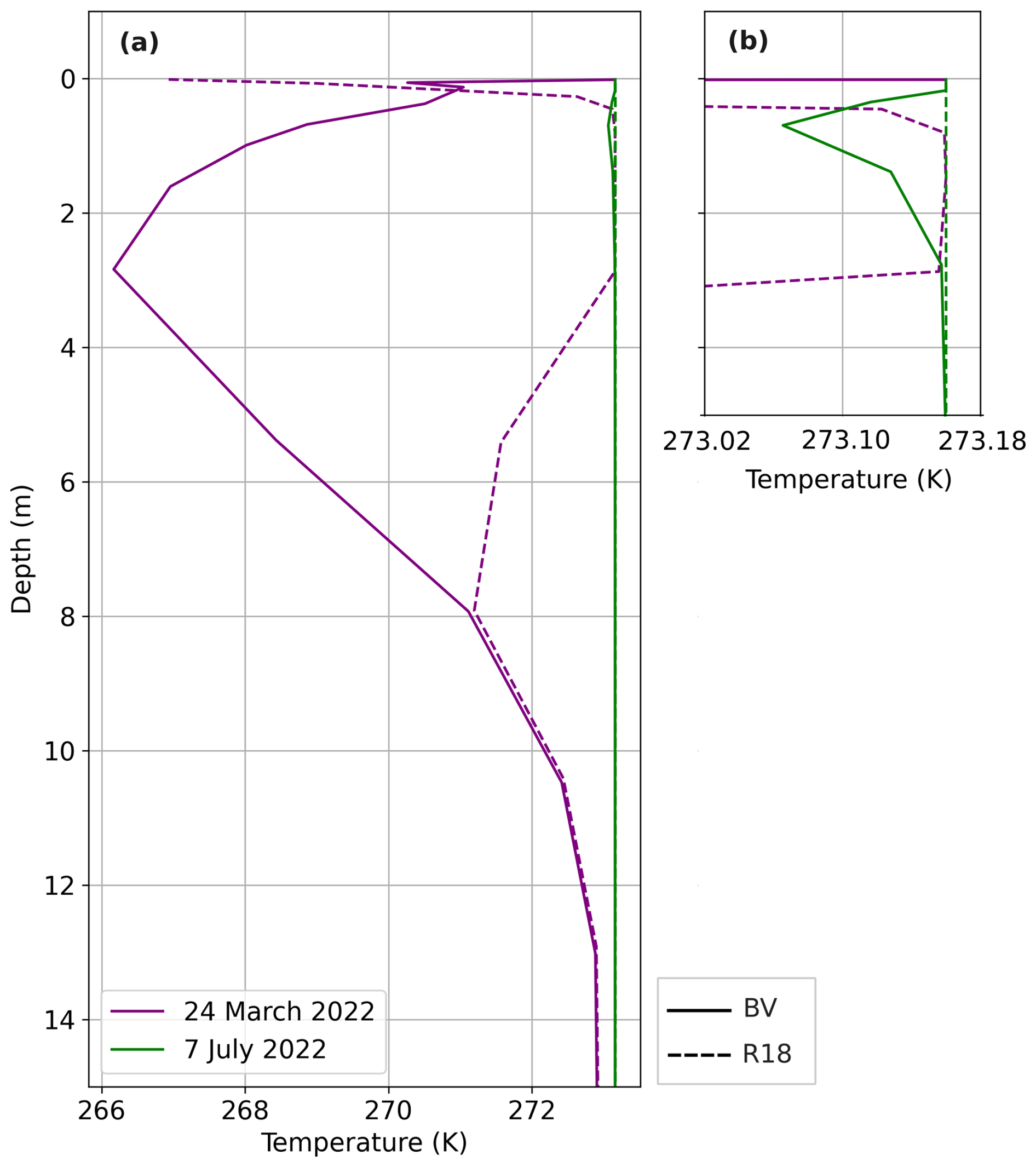
Figure 5 Vertical temperature profiles of the ice simulated at 6 p.m. during the pre-monsoon (24 March 2022, purple) and monsoon (7 July 2022, green) periods. Solid lines represent simulation performed with BV_default version, dashed lines correspond to R18 simulation. Panel (a) shows the depth profiles of the first 14 m, while panel (b) provides a zoomed-in view of the upper layers (5 m) to highlight differences in the monsoon period.

The thermal structure of the glacier explains these seasonal differences in mass balance between models. The temperature profiles at 6 p.m. (Fig. 5) reveal contrasting behavior between pre-monsoon and monsoon periods. During pre-monsoon (24 March 2022), BV_default (purple thick line) maintains a temperate surface that rapidly cools to 266 K at 3 m depth before warming to 271 K at 8 m. In contrast, R18 (purple dashed line) exhibits a colder surface (267 K) that quickly warms to 273.15 K at 0.7 m depth before converging with temperature simulated by BV_default, at greater depths (8 m).

During pre-monsoon periods, R18 handles the warming of the ice column differently than BV_default. In R18, meltwater refreezes immediately in the deeper cold ice layers until the entire column becomes temperate. This process effectively traps heat within the ice column through latent heat release at depth. In contrast, BV_default confines water to the surface where it refreezes only during nighttime cooling periods. This fundamental difference in thermal energy distribution causes BV_default to maintain a warmer surface temperature while limiting heat transfer to deeper layers. This warming effect dominates early in the season, primarily because the thermal profile of the glacier still reflects cold winter conditions.

During monsoon (7 July 2022, green lines), both model versions show nearly identical thermal profiles, with R18 maintaining 273.15 K throughout, while BV_default shows only minor cooling to 272.08 K between 0.6–0.8 m. This thermal homogeneity eliminates R18's ability to refreeze meltwater at depth, while BV_default continues to benefit from nocturnal surface cooling. As the monsoon progresses, the buffer's role shifts as its refreezing capacity becomes increasingly influential, counteracting daytime ablation and reducing overall annual mass loss by 0.1–0.2 m w.e. depending on meteorological conditions. This seasonal transition from a “melt-dominated” regime to a “refreeze-dominated” regime explains the reversal in mass balance trends between the two model versions.

4.2.2 Impact of the implementation across seasons

Figure 6 shows the seasonal evolution of the mass balance over the different periods of the hydrological year 2021–2022. Each subfigure corresponds to a representative 7-days period for the winter, pre-monsoon, monsoon, and post-monsoon seasons, highlighting the key differences between the model versions (BV_default and R18).

• Winter period

  During the winter period (December to March), the buffer remains inactive as the surface is entirely covered by snow throughout the sub-period (hatched area). Additionally, the consistently low temperatures (mean daily surface temperature: −10 °C) prevent melting, and the absence of rainfall results in no significant mass fluxes. As a consequence, no differences are observed between model versions during this season (Fig. 6a).

• Pre-monsoon period

  The pre-monsoon period marks the transition from cold to temperate ice with distinct model behavior (Fig. 6b). During initial days of the sub-period, melt in R18 is immediately refrozen, whereas in BV_default melt is stored as the buffer increases during the day and then this stored water is refreezed during the night (as seen in Sect. 4.1).

  This timing difference stems from how each model handles the thermal transition of the upper ice column (first 10 m) from winter cold to temperate conditions. In March, as winter transitions to spring, the upper ice column starts warming due to rising air temperatures (mean March air temperature: −10 °C). Winter conditions have left the upper 10 m of the glacier 15 °C colder than deeper layers (not shown), with this cold anomaly slowly diffusing downward. In R18, once melting begins (mid-March), refreezing occurs immediately in cold upper layers until ice becomes temperate. In contrast, BV_default confines refreezing to the top 50 cm during nighttime only, preventing deeper refreezing and modifying the surface energy balance. As a result, R18 transitions from cold to temperate ice approximately 2 months faster than BV_default.

• Monsoon period

  During the monsoon period (Fig. 6c), both model versions simulate similar melt and rainfall patterns, but differ in nighttime processes. In BV_default, stored water refreezes when temperatures drop, with complete refreezing on three nights and partial refreezing (20 %–50 %) on remaining nights. In R18, almost no refreezing occurs.

  When snowfall occurs during the monsoon (Fig. 6d), the buffer completely empties as snowfall alters necessary conditions for buffer existence. Consequently, both models show similar mass balances as the buffer's influence is neutralized.

  During monsoon periods without refreezing conditions (Fig. 6e), the buffer fills to its maximum capacity (0.01 m w.e.) due to rainfall and meltwater input. Persistent warm or cloudy night conditions (85 % of nights with surface temperature equals to 0 °C during the sub-period) prevent significant refreezing and maintain a temperate surface. The mass balance derivative remains negative with nearly identical behavior between models. Heat conduction from buffer to surface is negligible, explaining why BV_default does not induce more melt than R18.

• Post-monsoon period

  In the post-monsoon period (Fig. 6f), melt rates decline significantly (from 0.04 m w.e. d⁻¹ in monsoon to 0.007 m w.e. d⁻¹), reducing contributions to the buffer. Meltwater input is limited to 1–2 h d⁻¹ (versus 8–12 h during monsoon), and these reduced volumes rapidly refreeze overnight as surface temperatures remain below 0 °C.

Refreezing during this period occurs within 2–3 h after sunset, resulting in 0.007 m w.e. of refreezing per night (100 % of daily melt). This rapid refreezing slightly increases surface mass balance, though the effect remains limited compared to pre-monsoon and monsoon seasons.

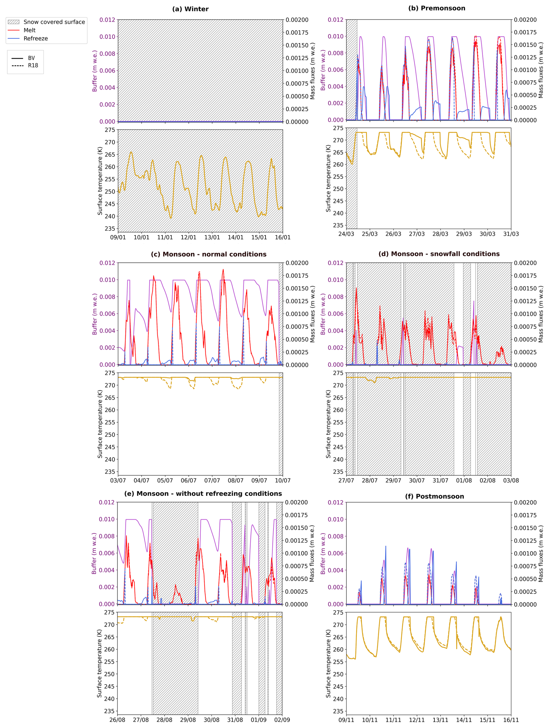
Figure 6 Seasonal variations of buffer, melt and refreeze (top panels) and surface temperature (bottom panels) for selected periods: (a) winter, (b) pre-monsoon, (c) typical monsoon conditions, (d) monsoon with snowfall events, (e) monsoon without refreezing conditions, and (f) post-monsoon. The top panels display melt (red), refreezing (blue), buffer (purple) while the bottom panels surface temperature for two datasets (BV_default in thick line, R18 in dashed line). Hatched areas indicate periods when the surface is covered with snow.

4.3 Model sensitivity

Model behavior and differences must be interpreted within the context of inherent modeling uncertainties, particularly regarding parameter values used in this implementation.

4.3.1 Impact of the drainage coefficient

The drainage coefficient significantly influences liquid water retention and associated mass balance components. Figure 7a shows how drainage values affect the buffer water content, with higher retention (coefficient near 1) maintaining maximum water content of 10 mm w.e., while lower retention (coefficient of 0.3) reduces maximum content to 0.5 mm w.e.

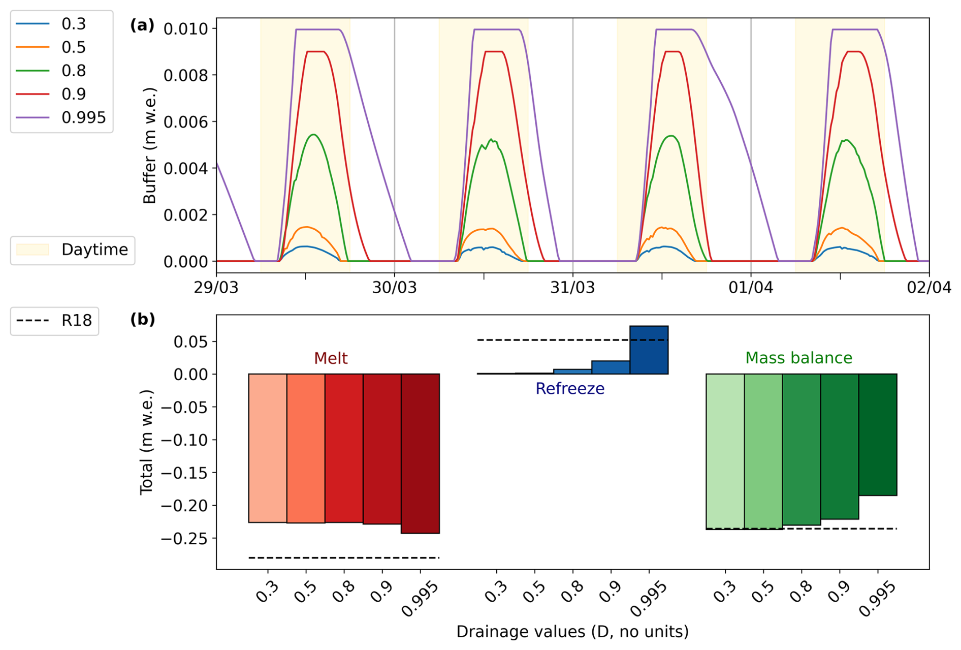
Figure 7 Analysis of the impact of drainage values (D) on mass balance for BV_tests version with fixed 0.35 albedo for ice, refrozen ice and liquid water over ice. (a) Temporal evolution of the buffer liquid water content (m w.e.) for different drainage values (D=0.3, 0.5, 0.8, 0.9, and 0.995) from the 29 March to the 6 April 2021–2022. Yellow shaded areas indicate daytime (6 a.m. to 6 p.m.). Vertical gridlines mark midnight, with minor ticks at noon. (b) Total mass balance (m w.e.) for different drainage values, divided into three components: melt (left, in red), refreezing (center, in blue), and the overall mass balance (right, in green). The dashed line represents values for R18 version. Negative values in the mass balance indicate a net loss.

The drainage coefficient regulates the balance between refreezing and melt volumes (Fig. 7b). A high coefficient (0.995) increases refreezing by 98 % compared to a low coefficient (0.5) due to greater liquid water retention in the buffer. During this period, R18 exhibits total melt of 0.27 m w.e., while BV_tests shows reduced melt between 0.22–0.23 m w.e., demonstrating the buffer's protective role.

The combined effects of additional refreezing and reduced melt directly impact mass balance outcomes. Lower drainage coefficients produce more negative mass balances (−0.22 m w.e. for coefficient 0.3 versus −0.15 m w.e. for coefficient 0.995). Under high drainage conditions (coefficients 0.3 to 0.8), the final mass balance becomes nearly identical between models (−0.22 m w.e. for both). However, under low drainage conditions, BV_tests produces a significantly less negative mass balance (−0.15 m w.e.) compared to R18 (−0.22 m w.e., 31 % difference), highlighting how low drainage enhances refreezing and mitigates mass loss.

4.3.2 Sensitivity of mass balance to buffer capacity and drainage coefficient

We tested the sensitivity of the mass balance to variations in the maximum buffer capacity (z_max,buff) and the drainage coefficient (D). Across all tested values, the maximum difference in annual mass balance was 0.84 m w.e., representing 17 % of the annual mass balance (Fig. 8).

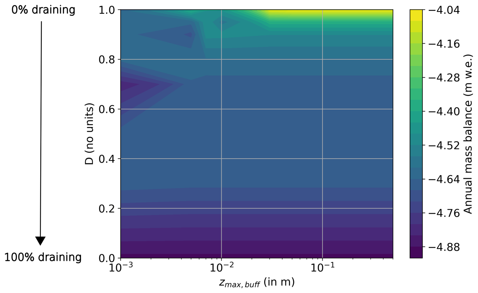
Figure 8 A contour plot showing the sensitivity of the annual mass balance (m w.e.) for 2021–2022 to variations in the buffer maximum capacity (z_max,buff) on the x-axis (logarithmic scale, in m) and the drainage coefficient (D) on the y-axis (linear scale, no units) for BV_tests version with fixed 0.35 albedo for ice, refrozen ice and liquid water over ice. The colour scale represents the annual mass balance, with values ranging from approximately −4.88 to −4.04 m w.e. Note that D=0 represents 100 % drainage while D=1 represents 0 % drainage, as indicated by the arrow on the left side.

Drainage coefficient sensitivity shows a threshold-dependent response. For values below 0.8, the influence on mass balance remains limited (differences < 0.1 m w.e. across simulations). However, for coefficients exceeding 0.8, the mass balance becomes progressively less negative as D approaches 1. At D=0.95 and z_max,buff > 3 mm, the reduction in mass loss reaches −4.16 m w.e. compared to −4.64 m w.e. in R18 or −4.04 m w.e. in BV_default with D=0.995.

The sensitivity to z_max,buff is more pronounced for values between 10⁻³ and $\mathrm{3}\times {\mathrm{10}}^{-\mathrm{2}}$ m, where an increase of 0.01 m w.e. in the maximum capacity results in a 10 % less negative mass balance.

Beyond $z_{\max ,\mathrm{buff}}=\mathrm{0.01}$ m and D=0.9, the mass balance stabilizes around −4.0 m w.e., indicating a saturation point where further parameter increases have negligible effect. This suggests physical limits on water storage and drainage efficiency.

4.3.3 Albedo

We systematically evaluated mass balance sensitivity across albedo values for both refrozen ice and liquid water on ice. The results obtained demonstrate that the albedo of liquid water on ice exerts a dominant influence on annual mass balance, with higher albedo values resulting in significantly less negative mass balances (ranging from −4.71 to −4.17 m w.e.; Fig. 9a). This represents a 11 % variation in annual mass balance across the tested range. Conversely, variations in refrozen ice albedo produce minimal impact (<0.1 m w.e., less than 2 % variation) across the same albedo range. This sensitivity difference stems from contrasting surface exposure durations: refrozen ice persists for only 2-3 h before melting and is mainly a thin layer, while liquid water-covered ice remains exposed for approximately 80 % of the surface time from March to October (see the Supplement, Sect. S5). However, the albedo effect of liquid water is moderated by the fraction x, which weights the relative contributions of ice albedo and liquid water albedo in the overall albedo calculation.

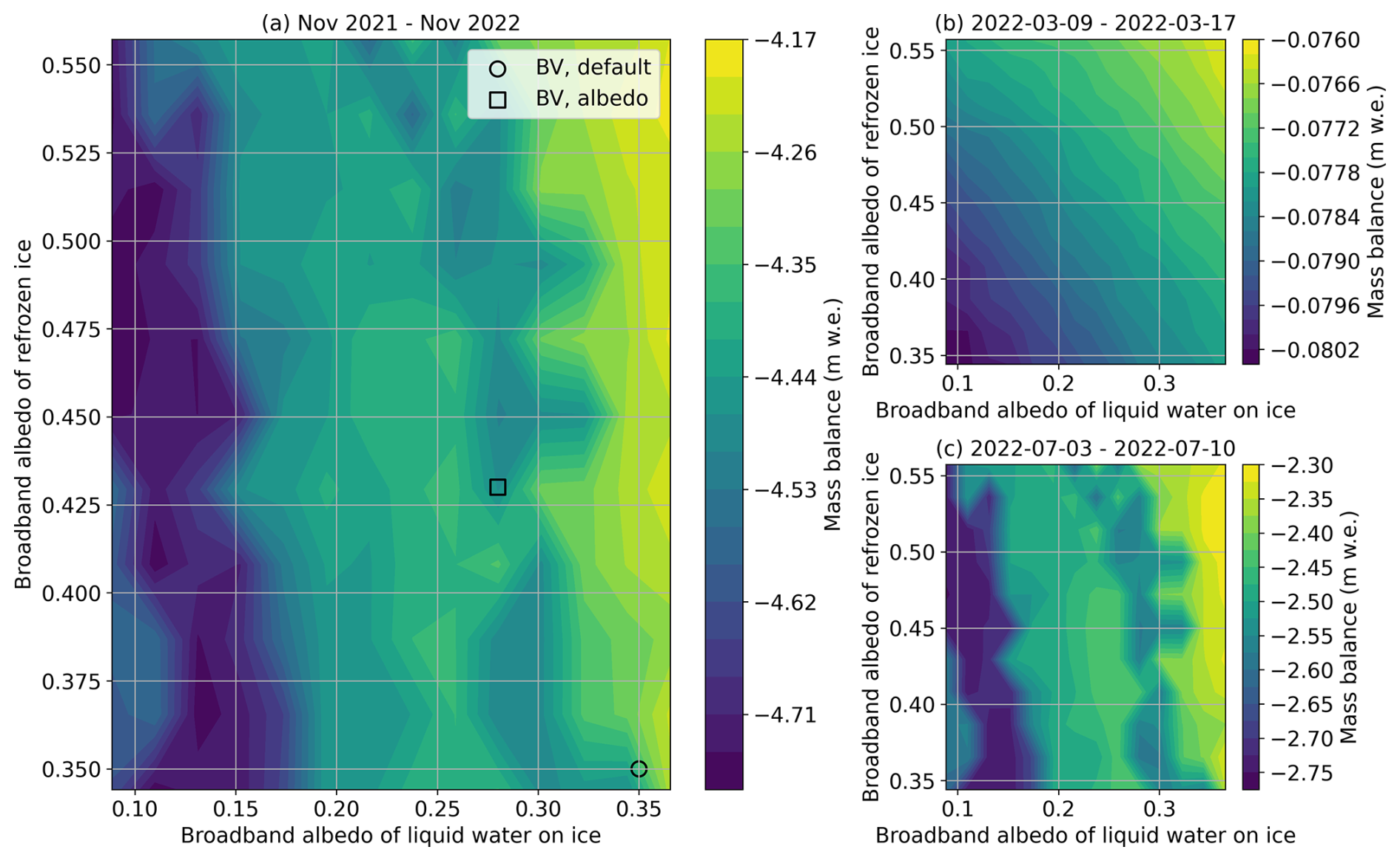
Figure 9 A contour plot showing the effect of broadband albedo values for refrozen ice (vertical axis) and liquid water on ice (horizontal axis) on the annual (a) or subperiods (b and c) mass balance (colour scale) for BV_tests version with x=0.2, D=0.995 and z_max=0.01 m. The subperiods are from the 9 March to the 17 March 2022 in (b) and from the 3 July to the 10 July 2022 in (c). The albedo values range from 0.1 to 0.35 for the liquid water over ice and from 0.35 to 0.55 for the refrozen ice in increments of 0.04 for both parameters. The square and circle points are indicating values for BV_albedo and BV_default respectively.

The influence of albedo is contingent on surface state, and thus season. By selecting a period in which the majority of the surface is composed of refrozen ice, as illustrated in Fig. 9b, a significant influence of the refrozen ice albedo can be observed (up to 4 % variation during this period). During that period, liquid water over ice exerts a similar influence (up to a 4 % variation). During periods when liquid water over ice dominates (Fig. 9c), which means that liquid water over ice occurs for more than 60 % of the of the time during this subperiod, the variation is similar to the annual graph, with liquid water albedo showing an even more dominant influence (up to 18 % variation over the period).

The annual scale sensitivity test is particularly influenced by periods of significant mass balance changes. In March, the albedo effect of refrozen ice may be a contributing factor to mass balance variations; however, the magnitude of these variations is comparatively negligible in relation to those observed during pre-monsoon or monsoon periods, when liquid water becomes the predominant surface state.

5 Discussion

The implementation of a surface liquid water reservoir on top of ice significantly affects both the timing and the amplitude of glacier surface processes. Our results demonstrate that accounting for temporary water storage alters the simulated energy and mass balance of glaciers. This section discusses the implications of these results, their limitations, and potential applications in future climate scenarios.

5.1 Buffer implementation

5.1.1 Limitations

The buffer implementation models surface water retention on glaciers while balancing realism with computational feasibility. Built on the Crocus framework within a 1D approach, this implementation offers key advantages for numerical modeling, particularly maintaining scheme stability through end-of-timestep heat flux calculations and representing inherently sub-grid processes. The approach captures surface water heterogeneity within individual grid cells while preserving computational efficiency and numerical robustness.

For energy balance calculations, our implementation assumes that ice remains the dominant surface material, even when liquid water is present. We treat the surface as ice for all energy balance processes except albedo and thermal conduction. This approach avoids significant changes to the model, since water coverage remains minor relative to ice coverage (i.e. <20 % in this study). However, it introduces limitations when large amounts of water accumulate in the buffer layer that could invalidate our energy balance assumptions. Water substantially alters surface energy fluxes by changing surface roughness, turbulence patterns and radiation properties (Brock et al., 2000). These changes would imply that the surface should be treated as water-dominated rather than ice-dominated. In order to maintain the validity of our ice-dominated assumption, we deliberately limit the maximum reservoir capacity to 0.01 m w.e., ensuring that ice characteristics dominate the surface energy balance. The fraction x further modulates water storage to maintain a reasonable ice-surface assumption. The sensitivity to these parameters will be further discussed in Sect. 5.2. In order for the hypothesis to remain true, users must be careful about the choice of parameter values. For example, the model is not adapted for an x over 0.5.

The buffer response to snowfall and freezing rain presents a minor limitation due to the small volumes of liquid water involved. Our current implementation assumes that snowfall and freezing rain immediately empties the buffer, preventing mixed phase interactions. While reasonable for heavy snowfall, this assumption may not hold for light snowfall where liquid water could warm and partially melt new snow. At Mera Glacier, freezing rain occurs infrequently (25 events, draining 0.01 m w.e.), but snowfall-driven buffer drainage is more common (53 events, draining 0.15 m w.e.), particularly during the monsoon. The potential impact of incorporating energy exchanges would depend on precipitation, temperature and intensity, with outcomes ranging from additional liquid water refreezing to partial snow melting. However, given the relatively small buffer volumes involved (maximum capacity of 0.01 m w.e. by default), it is likely that this refinement would produce only minor adjustments to annual mass balance calculations without altering fundamental melt patterns.

Our model currently uses constant parameter values throughout the season, but temporal evolution would improve realism for glacier-scale hydrological studies. Both D and z_max,buff could be parameterized as functions of seasonal conditions rather than constant values. This approach would better capture the natural evolution of glacial drainage systems. Observational studies support the importance of seasonal drainage evolution. Huss et al. (2008) documented seasonal drainage system evolution in the Alps and found that drainage efficiency increases as the ablation season progresses. Fyffe et al. (2019) observed distinct seasonal phases in supraglacial hydrology on debris-covered Nepalese glaciers. They found inefficient early-season drainage that evolves into well-developed channel networks later in summer. Our model does not yet capture such temporal dynamics. However, it is not necessary to take this temporal dynamic into account, since we are studying surface processes where water percolation is not considered. Future studies using this implementation for detailed hydrological analysis or glacier-wide applications might need to incorporate seasonal parameter evolution.

5.1.2 Simulations at larger scale

While Crocus is primarily designed for snowpack modeling, this work advances its generalization to represent the snowpack-glacier continuum within a single framework. A typical challenge when representing snowpack and glacier as a single column involves treating liquid water percolation, which fundamentally differs between porous, permeable snow and dense, impermeable ice. Due to their specific focus and temporal scope, previous Crocus glacier studies, such as those focusing on snowpack processes (e.g., Lejeune et al., 2007 in the Andes) or covering short periods and glacier-wide (e.g., Dumont et al., 2012 at Saint-Sorlin glacier), are likely only negligibly impacted by this implementation. However, longer-term studies focusing on the Saint-Sorlin glacier over extended periods, such as Réveillet et al. (2018); Gerbaux et al. (2005), may increasingly experience impacts from this process. Specifically, Réveillet et al. (2018) discussed the importance of liquid water at the ice surface for the energy balance. These earlier studies ended in the 2000s or 2010s when melt rates were lower (Thibert et al., 2018) and ablation zones are bigger, resulting in more ice surface exposed (Naegeli et al., 2019). There was therefore less surface water and a reduced need for this implementation. However, most current snow-ice models lack proper representation of surface water storage on ice. This limitation may significantly impact recent and future studies of glacial ice under current and projected climate conditions. Future mass balance modelisation studies should include this process, especially in long-term projections, which, to the best of our knowledge, are not currently taken into account.

This analysis focuses on an important surface process that occurs on a fine scale, affecting only a small proportion of the grid cell (the fraction x). However, it has an annual impact up to 6 % on a single point on Mera Glacier. Future work would be to scale up this implementation both spatially and temporally across entire glaciers. This phenomenon might have a greater impact in regions with more rain or in zones of ablation with longer ice exposure during the year. Applying this buffer approach to any mountain glacier would provide insight into the potential for significant impacts under future climate scenarios, particularly given the evolving rain-snow limit and its effect on the precipitation phase (Fehlmann et al., 2018; Schauwecker et al., 2022; Guo et al., 2021). However, such large-scale applications require thorough observations of the processes involved, particularly albedo measurements, in order to properly constrain and validate implementation in diverse glacial environments.

5.2 Parameter sensitivity and observational constraints

The implementation presented in this study provides a physically based representation of surface water retention processes, which requires observational validation for reliable application. To avoid virtual glacier scenarios, we used Mera Glacier as a test case, taking advantage of its particular climatic context and existing parameter constraints from previous studies. This study, primarily aims to demonstrate the impact of this surface process and its relevance for glacier modeling. However the model development relies on observational data for accurate calibration and evaluation before it can be applied to any glacier.

Key parameters, including z_max,buff, x, D and surface-specific albedo values, remain poorly constrained by observations, likely owing to the fine spatial scale of these surface processes. Dedicated field campaigns focused on these processes would provide valuable insights to substantially reduce model uncertainty.

The model is designed to allow users full flexibility in defining these key parameters, enabling calibration specific to each glacier and thereby supporting global applicability. In this study, sensitivity tests were conducted on these parameters to address the lack of observational constraints and to highlight the care needed when choosing their values. Each of the three parameters is discussed in detail below.

5.2.1 Fraction x

x is constrained to ensure physical consistency in the surface energy balance. Most surface energy fluxes are computed assuming an ice-covered surface, except for albedo and thermal conduction. However, when the liquid water fraction becomes too large, this assumption no longer holds. To prevent this inconsistency, we advice limiting x to values below 0.5, which ensures that ice remains the dominant phase in each grid cell. Sensitivity tests were performed on x, but with x lower than 0.5 and for D=0.995 (not shown), the sensitivity is lower than 2 % and is largely dependent on the albedo values chosen for the different surfaces.

This limit is in agreement with some existing observations. For example, melt pond fractions above 0.5 are rarely reported during the Arctic melt season (Skyllingstad et al., 2015). Grenfell and Maykut (1977) provide specific measurements of pond fractions (related to the parameter x described in Sect. 3.2.2) from Greenland. Given that these observations originate from Arctic regions (typically flatter than mountain glacier environments) the derived thresholds may be overestimated in the context of our study. Nevertheless, such values are expected to be strongly site-specific and not readily transferable, underscoring the need for local observations to ensure accurate calibration.

5.2.2 Drainage coefficient D

The sensitivity to D is particularly influential, controlling the residence time of liquid water and subsequently affecting both energy absorption and refreezing. Variations in D by 10 % alter annual mass balance by up to 10 % in our simulations (see Sect. 4.3.1), aligning with findings from Lüthje et al. (2006) or Skyllingstad et al. (2015) who identified drainage parameters as critical factors in melt pond evolution on sea ice.

In Greenland ice sheet models, similar drainage coefficients typically range from 0.8 to 0.995 (Lefebre et al., 2003; Fettweis et al., 2017), with MAR commonly using values close to 0.995 combined with a maximum residence time of 18 h (version 3.14) to ensure that liquid water does not remain longer than one night. However, glacier environments differ substantially from ice sheets in their surface roughness, slope, and drainage networks. Irvine-Fynn et al. (2011) documented highly variable drainage efficiencies in mountain glaciers, suggesting that a single static drainage coefficient may oversimplify actual conditions.

Due to the high sensitivity and possible significant spatial variability of this coefficient, which make it site-dependent, we recommend careful selection of its value and conducting sensitivity tests to ensure its relevance for the specific study site.

5.2.3 Maximum capacity z_max,buff

z_max,buff establishes critical thresholds for water retention with clear implications for model sensitivity. Values exceeding 0.01 m lead to limited additional impact on mass balance (Fig. 8), providing useful constraints for future model implementations. To our knowledge, no direct field observations of surface water pond heights exist for temperate mountain glaciers similar to our study site, highlighting a knowledge gap that our findings could help address. Existing literature on surface water depths provides context but from very different glaciological settings. Sneed and Hamilton (2011) report depths of 0.2–3 m of supraglacial melt ponds, while Cooper et al. (2018) suggest approximately 15 cm of meltwater storage in porous ice in Greenland. Similarly, studies by Cook et al. (2016) in Svalbard and Irvine-Fynn et al. (2017) on debris-covered glaciers examine different water systems that differ substantially from our temperate mountain glacier context. Although region-specific observations would help to refine estimates of buffer capacity, the results of the sensitivity tests suggest that constraining water storage to 0.01 m is a justifiable and practical assumption in the absence of additional observations.

5.2.4 Albedo

Albedo is the most sensitive parameter requiring observations for accurate calibration. While the parameter D shows the strongest influence across the full tested range, this effect becomes less dominant when D is restricted to more realistic values (i.e. >0.95). In that case, albedo variations have the greatest impact, leading to up to 18 % change in mass balance. This is consistent with numerous studies identifying solar radiation as the primary energy source controlling glacial melt rates (e.g., Brock et al., 2006; Johnson and Rupper, 2020). Our results specifically show that changes in the albedo of the three surface types we model – bare ice, liquid water on ice, and refrozen ice – can significantly alter annual mass balance, with variations in liquid water albedo alone changing mass balance by up to 18 % (Fig. 9c). This sensitivity emphasizes the importance of accurately representing the optical properties of these different ice surface conditions, as current observational gaps contribute to limited understanding.

Bare ice albedo has been characterized using both satellite-based observations and in situ measurements. While remote sensing enables large-scale monitoring of ice albedo (e.g., Brun et al., 2015; Naegeli and Huss, 2017; Naegeli et al., 2019), it struggles with liquid water on ice or refrozen ice surfaces due to constraints in spatial resolution and spectral signature. Conversely, in situ broadband measurements provide precise point-scale data, yet they are inadequate to represent the pronounced spatial and temporal heterogeneity observed on glacier surfaces (Hartl et al., 2020). Additional observations aimed at characterizing the albedo of liquid water and refrozen ice surfaces would require dedicated field campaigns and careful methodological design.

The optical properties of ice surfaces with or without liquid water are highly complex and dynamic. Field measurements by Grenfell and Maykut (1977) and more recent work by Tedstone et al. (2020) demonstrate that liquid water on ice surfaces can reduce albedo by 20 %–70 %, depending on water depth, substrate characteristics, and impurity content. Our sensitivity testing range of 0.1–0.35 for liquid water albedo encompasses these observations but highlights the need for site-specific measurements to constrain this parameter. The albedo reduction occurs because water fills surface irregularities, creating a smoother surface that reduces light scattering and increases absorption (Gardner and Sharp, 2010). The refrozen ice presents additional complexity in albedo representation. Our simulations test refrozen ice albedo values from 0.35–0.55, based on observations by Traversa and Di Mauro (2024) who found that refrozen ice can increase albedo by up to 23 % compared to bare ice.

However, the impact of refrozen ice albedo is limited, in our model, as these surfaces persist for only 2–3 h before re-melting and mainly represent a thin layer with a very low r_frac,i on average (see Fig. S5 in the Supplement, Sect. S5). Under different meteorological conditions, this effect might be more significant. It is also important to note that sensitivity tests are performed on Mera Glacier, which exhibits a relatively high bare ice albedo (0.35) compared to many other glaciers (e.g., 0.15–0.2 at Saint-Sorlin Glacier (Dumont et al., 2011)). As a result, the sensitivity observed in this study may be underestimated, underscoring the importance of careful calibration of albedo values in model applications.

Additionally, other surface characteristics, such as surface roughness, introduce complexity in accurately measuring and interpreting albedo. For instance, Hartl et al. (2020), Brock et al. (2006), and Larue et al. (2020) showed that micro-scale surface roughness can alter albedo independently of water content by changing the effective angle of incidence for solar radiation. Crocus currently uses a constant roughness parameter, which limits its ability to capture temporal and spatial variations in surface characteristics. Furthermore, the effect of impurity content and biological activity linked to surface liquid water conditions would deserve dedicated study. Light absorbing impurities such as mineral dust and black carbon significantly reduce ice albedo (e.g., Di Mauro et al., 2017; Volery et al., 2025; Gilardoni et al., 2022), yet their interactions with liquid water at the ice surface remain poorly documented. Liquid water potentially facilitates both impurity accumulation through ponding (Marshall and Miller, 2020) and biological growth (Tedstone et al., 2020). Our model does not currently account for these processes, potentially underestimating albedo reduction in certain scenarios.

Finally, the temporal evolution of surface conditions also challenges albedo parameterization in glacier models. Ryan et al. (2018) documented substantial diurnal and seasonal variations in ice albedo related to changing surface conditions, while Sicart et al. (2001) and Picard et al. (2020) emphasized measurement biases related to solar zenith angle and surface slope. Our model applies fixed albedo values for each surface state, neglecting these temporal dynamics. Future improvements could incorporate time-dependent albedo evolution to better capture these processes.

Whether to improve the parameterization of albedo values for different surface types in the model or to advance the albedo scheme for better representation of spatial and temporal variability, targeted and dedicated field measurements are essential.

5.3 Model transferability and glacier evolution under climate change

5.3.1 Transferability of the model development to other glaciers

The buffer layer implementation is based on physical representations of water retention at the ice surface (water accumulation, thermal exchange, albedo modification, drainage, and refreezing) and was developed without region-specific calibration to remain broadly transferable. However, buffer parameters still require site-specific tuning, as they depend on local conditions (e.g. glacier geometry, surface topography, climate conditions). For instance z_max varies with surface roughness and microtopography, D reflects local drainage efficiency influenced by crevasse density or channel development, x adjusts for surface water coverage (constrained to x<0.5 to maintain ice dominance), and albedo values depend on sediment concentration, ice crystal structure, and impurity content (e.g. Gardner and Sharp, 2010; Dadic et al., 2013). Additional care may be needed for instance for polar regions due to the prevalence of superimposed ice formation and the potential for seasonal meltwater storage within ice layers (Cooper et al., 2018), which differ from the surface-only water storage represented by the buffer. Consequently, parameter calibration requires careful tuning to ensure reliable model performance and parameters are intentionally left free for users to adjust, preferably calibrated with local observations to ensure the proper functioning of the buffer approach.

More generally, the question of model transferability applies to Crocus beyond its original alpine context (Vionnet et al., 2012). Although built on a robust physical basis, Crocus still requires calibration when applied in contrasting climatic environments. Previous studies have demonstrated its use in regions such as the tropical Andes (e.g. Lejeune et al., 2007; Wagnon et al., 2009) and the Arctic (e.g. Royer et al., 2021) where adjustments to some key processes (e.g. fresh-snow density or thermal-conductivity parameterizations) were necessary. In the present study, however, only the ice surface is considered, which makes the approach more easily transferable for the specific case of surface meltwater retention.

5.3.2 Glaciers mass balance evolution in a warming climate

Our results demonstrate that buffer physics reduce annual mass loss of Mera Glacier by 0.1–0.2 m w.e. under current climate conditions, with implications that will intensify under future warming scenarios. As global temperatures rise, high mountain regions will experience increased melting and shifts in the snow-rain limit (Hock et al., 2019; Schauwecker et al., 2017). The frequency and intensity of precipitation events at glacier elevations are expected to increase (Pritchard, 2019), potentially enhancing liquid water availability for surface water retention processes.

Climate warming will significantly increase the importance of surface water processes on mountain glacier mass balance. Kraaijenbrink et al. (2017) indicate that a 2 °C temperature increase will likely result in mass losses between 49 %–64 % in the Himalayan region, consequently increasing supraglacial water accumulation due to enhanced melt rates. Under such conditions, buffer effects could substantially modify mass balance responses, with prolonged meltwater retention potentially mitigating short-term ablation through refreezing processes.

The increased presence of liquid water on glacier surfaces creates a complex competition between opposing processes affecting mass balance, as shown in this study. On one hand, liquid water accelerates melting through reduced albedo and enhanced conduction during “melt-dominated” regimes when surface temperatures remain consistently above freezing. On the other hand, refreezing processes add mass through buffer formation during “refreeze-dominated” regimes when diurnal or seasonal temperature cycles promote ice formation. This competition between melt enhancement and mass addition through refreezing represents a fundamental control on glacier response to warming. This new implementation is essential for a better understanding of this phenomenon and for constraining it for future projections.

Regional variations in accumulation patterns will significantly influence how buffer processes respond to climate change. Summer accumulation glaciers, such as those found in the Andes (Rabatel et al., 2013) or the Himalayas (Fujita, 2008), receive most of their snowfall during the warm and wet season, when melting also occurs. This means that snow can fall while the glacier is already melting. In contrast, winter accumulation glaciers like those in the Alps get most of their snowfall during the cold season, when limited melt occurs. Warming trends may progressively shorten the duration of refreezing phases during ablation seasons, as already observed on low-elevation Alpine glaciers (Gabbi et al., 2014), while simultaneously increasing the frequency and persistence of surface water. This shift would enhance melt through feedback associated with water's lower albedo compared to bare ice, potentially reducing the net mass-conserving effect of buffer processes.

The net impact of these competing processes likely varies substantially with regional climate and topographic context, making buffer effects difficult to predict without site-specific analysis. This variability underlines the need for comparative, multi-site studies to better constrain the role of surface water retention in glacier mass balance evolution under different climate scenarios and to determine whether buffer processes will serve as a significant feedback mechanism in future glacier response to warming.

6 Conclusions

This study presents the implementation of a physically-based surface liquid water reservoir within the Crocus model. The approach allows for supraglacial water storage, with a simple parameterization of drainage controlled by surface slope. It also includes the thermal effect of water retention and its impact on albedo. At the core of this implementation is a virtual surface layer referred to as the buffer, which temporarily stores liquid water between time steps without adding to the complexity of the model’s physical layering. This buffer captures the main processes of surface water retention in ice roughness and activates only under specific conditions, ensuring a realistic yet manageable simulation of supraglacial water retention. This development provides a flexible and realistic framework to represent key surface processes (such as melt, refreezing and drainage), using parameters that can be adapted to local conditions based on available observations.

To illustrate the relevance of this development, we applied the model to a study case (Mera Glacier, Nepal). Results show that supraglacial water retention can significantly influence the glacier's energy and mass balance, with surface refreezing reaching up to 100 % of daily melt in some periods. This leads to a reduction in annual mass loss by 0.1–0.2 m w.e., compared to simulations without surface water storage.

The impact of the buffer exhibits strong seasonal variations, oscillating between “melt-dominated” and “refreeze-dominated” regimes. During the pre-monsoon period, the presence of liquid water increases surface energy absorption and accelerates melting, resulting in a slight increase in mass loss. By contrast, during the monsoon and post-monsoon periods, cooler night-time conditions favor the refreezing of stored water, accounting for up to 40 % of daily melt. This significantly mitigates mass loss, explaining the lower annual ablation in simulations including the buffer. Because its effects vary with seasonal and meteorological conditions, water retention is highly site-specific and likely to evolve under changing climate conditions.

The albedo representation is a key component of the model. It explicitly accounts for the distinct albedo values of refrozen ice, bare ice and liquid water, which have so far been scarcely considered in mass balance models. Albedo is computed as a weighted average based on the respective surface fractions of these components. The model provides a novel and flexible framework that allows users to adjust parameter values based on data availability or specific study objectives. It also highlights the critical need for targeted albedo measurements in the field.

As climate warming intensifies, with expected increases in melt and rainfall frequency, the presence of surface liquid water will become even more prevalent. Our study suggests that neglecting these processes could underestimate mass loss, reinforcing the need for improved model representations of surface liquid water storage.