Changes in 1958–2019 Greenland surface mass balance are attributable to both greenhouse gases and anthropogenic aerosols

Greenland Ice Sheet (GrIS) mass loss is a main contributor to rising Global Mean Sea Level (GMSL), exhibiting decadal variability due to surface mass balance (SMB) changes. Greenhouse gases (GHG) have long been identified as a key driver of GrIS mass loss through warming-induced runoff. However, there has not been a formal attribution of historical GrIS SMB changes to GHG and the potential role for other forcings such as anthropogenic aerosols (AAER). Here, we use the Community Earth System Model version 2 large ensemble and single forcing large ensemble (CESM2-LE and CESM2-SFLE) to formulate a detection and attribution analysis for historical GrIS SMB changes. We show that the decadal variability of SMB is forced by historical radiative forcing attributable to both GHG and AAER through their forced changes of runoff. This highlights that, in addition to the frequently mentioned GHG, AAER also contributes to SMB changes during the historical period. GHG influences GrIS runoff mainly through long-term radiatively-forced warming, while AAER influences it through the decadal variability of atmospheric circulation that projects onto a Greenland blocking pattern, leading to relative cooling from cyclonic circulation over Greenland pre-1980 and relative warming from anti-cyclonic circulation thereafter. The attribution of SMB, and specifically runoff, to AAER has a lower signal-to-noise ratio (S $/$ N) than the attribution to GHG due to both a weaker signal and wider confidence intervals. The lower S $/$ N in attributing runoff changes to AAER is partly due to a smaller temperature response in AAER than in GHG and partly due to a mean state temperature dependency of the runoff sensitivity. In simulations with only AAER, the climate is colder than in simulations with all forcings or only GHG, leading to more time below freezing when temperature variations do not affect runoff as much. We resolve this issue by comparing simulations with all forcings with simulations in which everything-but-AAER is changing, thereby stressing the need to account for mean state dependencies when conducting detection and attribution with single forcing simulations.

1 Introduction

The global mean sea level (GMSL) has been rising at an averaged rate of 1.56 mm yr⁻¹ since 1900 (Frederikse et al., 2020a; Hay et al., 2015; Church et al., 2011) and has accelerated to 3.3 mm yr⁻¹ since the 1990s (Chen et al., 2017; Church et al., 2011). A growing contribution to GMSL rise is from the ocean mass increase (barystatic sea level rise), due to freshwater input to the ocean from terrestrial water, mountain glaciers, and polar ice sheets, including both the Greenland Ice Sheet (GrIS) and Antarctic Ice Sheet. Glaciers remain the least constrained component of the climate change-driven sea level rise (IPCC, 2023). Among these glacial GMSL sources, the GrIS is one of the largest barystatic sea level contributors to GMSL since 1900 (accounting for 29 % of the total GMSL increase) (Frederikse et al., 2020a). Along with contributing to GMSL rise, GrIS mass loss can further increase regional sea level rise rate, such as for the North American East Coast (Mitrovica et al., 2001), resulting in higher risk of coastal flooding (Wdowinski et al., 2016).

GrIS mass loss comes from two factors (Mouginot et al., 2019): (1) changes in the surface mass balance (SMB), defined as the difference between precipitation, evaporation/sublimation, and runoff, and (2) changes in ice discharge related to glacial dynamics, manifested in calving and ocean melting trends. Observational records show that declining GrIS SMB has become an increasingly important contributor to rising GMSL in recent decades (Enderlin et al., 2014; Kjeldsen et al., 2015; Mouginot et al., 2019) and GrIS SMB change is identified as the largest source of GMSL uncertainty in future projections (Pattyn et al., 2018). Thus, understanding why the SMB has changed historically can be informative for projecting future changes of GMSL due to GrIS mass loss.

GrIS SMB reduction has been linked to rising air temperature over Greenland, as warming leads to more surface melting and runoff (Trusel et al., 2018; van Kampenhout et al., 2020; Thompson-Munson et al., 2024). Greenhouse Gases (GHG) amplify warming over the Arctic (Wu et al., 2024), and the consequent runoff increase is consistent with the monotonic long-term decline in GrIS SMB projected for the future under strong radiative forcing scenarios (Hofer et al., 2020). However, there has not been a formal attribution of historical GrIS SMB changes to radiative forcing, despite the emerging signal from GHG-induced global mean temperature warming in recent decades (Deser et al., 2020b). The GrIS SMB decline since the 1990s has also been linked to the increasing frequency of subsidence-induced warming from Greenland blocking, itself linked to the negative phase of the North Atlantic Oscillation (NAO). NAO-related GrIS SMB change has thus far been treated as internal variability on decadal time scales (Sherman et al., 2020; Brils et al., 2023; Hanna et al., 2022). However, new literature attributes the negative NAO transition to anthropogenic aerosols (AAER; Dong and Sutton (2021)) and provides evidence of AAER-forced historical decadal variability for different aspects of North Atlantic climate, including storm tracks (Kang et al., 2024) and sea surface temperatures (SSTs; He et al. (2023)). We hypothesize that internal variability might not be the only reason for the recent decadal GrIS SMB changes; instead, both GHG and AAER could have also contributed.

Unlike GHG, historical AAER emissions had a non-monotonic spatio-temporal trajectory, owing to, for example, the timing of social-economic development and air quality regulations in different countries (Persad et al., 2022). This heterogeneous characteristic of AAER has been argued to induce historical decadal variability in various aspects of the Earth's climate; prominent recent examples include tropical SST patterns (Hwang et al., 2024; Dittus et al., 2021; Takahashi and Watanabe, 2016), regional hydroclimate change (Kuo et al., 2025), and mid-latitude circulation (Dow et al., 2021; Oudar et al., 2018). Together with the literature supporting AAER-forced historical decadal variability of North Atlantic climate, we hypothesize that AAER contributes to GrIS SMB changes through its impacts on atmospheric circulation.

However, the forced response to AAER often has a low signal-to-noise ratio (S $/$ N) (Dittus et al., 2021; Oudar et al., 2018; Kuo et al., 2023), and so do externally forced NAO changes (McKenna and Maycock, 2021; Scaife and Smith, 2018). Different external radiative forcings can also create nonlinear (or non-additive) responses in the climate system (Simpson et al., 2023; Kuo et al., 2025). As such, nonlinear interactions between AAER and GHG forcings cannot be captured in the single forcing runs of AAER-only or GHG-only simulations. New climate model large ensembles are designed to better isolate subtle signals and responses to individual forcings from internal variability (Deser et al., 2020a). Therefore, in this study, we utilize the Community Earth System Model version 2 (CESM2; Danabasoglu et al. (2020)) large ensemble (CESM2-LE; Rodgers et al. (2021)) and its single forcing large ensemble (CESM2-SFLE) with both forcing-only and all-but-forcing experimental setups (Simpson et al., 2023) to better understand whether the historical decadal variability of GrIS SMB is forced by both GHG and AAER.

In this paper, we apply the detection and attribution (D&A) framework from Allen and Stott (2003) to formally assess whether historical radiative forcings can account for GrIS SMB changes between 1958–2019. We demonstrate that both GHG and AAER contributed to the 1958–2019 GrIS SMB changes and highlight a previously underappreciated source of uncertainty in D&A when the climate response has mean state temperature dependency. This mean state temperature dependency can lead to different S $/$ N for the attribution to GHG compared to AAER. Finally, we will discuss implications of these uncertainties for the general D&A framework.

2 Data and Methods

2.1 Data

2.1.1 Reference data

In this study, reconstruction data, reanalysis data, and a regional climate model simulation driven by reanalysis since 1958 are included as reference data for the historical period. Frederikse et al. (2020a)'s reconstruction for GrIS mass loss was used to assess the impact of SMB change on GrIS GMSL contributions since 1958. The Frederikse et al. (2020a)'s reconstruction data comes from a Monte Carlo simulation perturbing the known prior estimate based on three estimates of GrIS mass loss data, including a reconstruction from geological inference of historical ice sheet surface elevation (Kjeldsen et al., 2015), an input-output estimate (Mouginot et al., 2019), and a synthesis of satellite observations with a multi-method assessment (Bamber et al., 2018). With 5000 ensemble members, this reconstruction provides a range of observational uncertainty of the GMSL contribution from GrIS mass loss. To understand the drivers of the GrIS GMSL contribution, we use 1958–2019 annual mean SMB, precipitation (P), and runoff (R), averaged over the GrIS, from the polar regional climate model RACMO2.3p2 simulation forced with the reanalysis data sets from ECMWF Reanalysis (ERA), hereafter RACMO-ERA (Noël et al., 2022a). RACMO-ERA is run at 5.5 km resolution and statistically downscaled to 1 km (Noël et al., 2022a). This RACMO-ERA simulation has been compared against in-situ meteorological data and point measurements of GrIS SMB and showed good agreement with these observations (Noël et al., 2018). Here, these RACMO-ERA outputs are treated as the reference data to formulate a D&A analysis. Additionally, annual means of near-surface temperature at 2 m (TAS) and 500 hPa geopotential height (Z₅₀₀) from monthly gridded ERA5 reanalysis (Hersbach et al., 2020) are included to investigate the atmospheric drivers of the SMB changes.

2.1.2 CESM2 large ensemble and single forcing large ensemble (CESM2-LE and CESM2-SFLE)

CESM2-LE and CESM2-SFLE are used for the D&A analysis. CESM2 (Danabasoglu et al., 2020) is a climate model developed by the National Center for Atmospheric Research (NCAR). It includes a land ice model (CISM) (Lipscomb et al., 2019) of the GrIS at 4 km spatial resolution. CESM2-LE and CESM2-SFLE are run setups with a fixed ice sheet topography so that CISM does not feed back to other parts of the climate system but provides the finer grids to downscale SMB. CESM2 has been evaluated against observations and shown to capture the variability of GrIS SMB well (van Kampenhout et al., 2020; Noël et al., 2020, 2022a).

We take the 50-member ensemble from CESM2-LE (Rodgers et al., 2021) that is forced with the full historical radiative forcings (ALL), using smoothed biomass burning forcing (smbb). Each ensemble member differs from the others due to initial condition perturbations (see Rodgers et al. (2021)) to quantify the uncertainty originating from internal variability. CESM2-SFLE (Simpson et al., 2023) uses the same CESM2 version but instead of the ALL forcing, individual forcings are applied in isolation. We use the 15-member GHG and AAER simulations, as GHG and AAER are two dominant anthropogenic forcings for historical climate change (Deser et al., 2020b). In CESM2-SFLE, the GHG (AAER) simulation is forced with time-evolving GHG (AAER) forcing, with other forcing held fixed at 1850 levels (i.e., the forcing-only experimental setup). We also include the 10-member all-but-aerosols (xAAER; the all-but-forcing experimental setup) simulations and follow Deser et al. (2020b) to calculate the contribution of anthropogenic aerosols as the difference between ALL and xAAER (ALL-minus-xAAER). With xAAER and ALL-minus-xAAER, we can assess the robustness of D&A results given the potential non-additivity issue reported in Simpson et al. (2023).

We use the annual SMB, and monthly P, R, TAS, and Z₅₀₀ from these simulations. Monthly CESM2 outputs are converted to an annual sum (P, R) or annual mean (TAS, Z₅₀₀) to compare against annual SMB. The area-weighted SMB, P, R (unit: mm yr⁻¹) is summed over Greenland and divided by the global ocean area derived from the CESM2 land mask to convert into a GMSL equivalent (unit: mm GMSL equivalent per year). This GMSL equivalent is multiplied by 361.8 to convert to Gt yr⁻¹. Anomalies are calculated by removing the 1958–2019 climatological means for regression analyses.

2.2 Detection and attribution (D&A) approach

D&A is commonly performed with a regression of the observation (y) onto the fingerprint(s) of the external forcing (x_i) as

$$\begin{array}{}\text{(1)}& y=\sum _{i=\mathrm{1}}^m{\mathit{\beta }}_i{x}_i+{\mathit{ϵ}}_y\end{array}$$

where β_i is the scaling factor(s) to best match the time-dependent fingerprint(s) to the observation. The fingerprint(s) x_i are usually estimated by averaging many simulations (e.g., ensemble mean), and ϵ_y is the residual not explained by the simulated forced response (e.g., internal variability) (Allen and Stott, 2003; Swart et al., 2018). In this paper, we treat the RACMO-ERA simulation as y as there is no in-situ observation of GrIS SMB at the temporal and spatial coverages necessary for this D&A analysis; x_i are estimated by the ensemble mean of CESM2-LE and CESM2-SFLE. For the univariate case (i=1), x_i is estimated by the ensemble mean from ALL as x_ALL; for the bivariate case (i=2), x_i are estimated by the ensemble mean from GHG and AAER as x_GHG and x_AAER (or x_xAAER and x_{ALL-minus-xAAER}). Eq. (1) can be solved by performing an ordinary least squares (OLS) regression with y and x_i. In this case, we assume x_i is observed without uncertainty. When β_i is significantly larger than 0, the forced response from fingerprint x_i is considered detectable; when β_i is not significantly different from 1, the forced response is considered attributable to the fingerprint x_i. The significance level of β_i is usually determined from the distribution of β_i due to internal variability, estimated from climate models (e.g., from pre-industrial simulations (PiControl) or historical simulations from which the ensemble mean has been removed), and follows the IPCC guidance to indicate the significance of β_i and the confidence of attributing this signal to a given forcing(s).

In practice, x_i contains uncertainties, such as from the choice of climate models and the errors due to averaging over a finite number of ensemble members. A total least squares (TLS) regression is a common solution to perform D&A to account for uncertainty in x_i (Allen and Stott, 2003; Kirchmeier-Young et al., 2017; Schurer et al., 2013). Eq. (1) can be rewritten as

$$\begin{array}{}\text{(2)}& y=\sum _{i=\mathrm{1}}^m{\mathit{\beta }}_i(x_i-{\mathit{ϵ}}_{x_i})+{\mathit{ϵ}}_y\end{array}$$

where now, ${\mathit{ϵ}}_{x_i}$ is introduced to account for the uncertainties in simulated forced response in x_i. A singular value decomposition (SVD) on the system of equations can solve β_i in a deterministic way for the TLS regression (Allen and Stott, 2003).

The choice of whether to use an OLS or TLS regression should be made with caution, as TLS regression is not necessarily preferred over OLS for climate change D&A (McKitrick, 2023). For example, the deterministic solutions of TLS regression can be considered as a linear transformation of OLS regression coefficients and, mathematically, such a transformation could introduce an upward bias for the regression coefficients, leading to a potential false positive in D&A when determining β_i with TLS regression (McKitrick, 2023). Moreover, climate models have biases in simulating the internal variability, either too large or too small a magnitude, which makes estimating the significance level of β_i from internal variability based on that from climate models an imperfect approach.

In this study, we instead construct a Bayesian TLS regression to reduce bias and account for the uncertainty from using a climate model large ensemble from a single model (CESM2-LE and CESM2-SFLE). We first construct an ensemble of numerical experiments for an ideal case of one-dimensional linear regression y=βx where both sampled data y and x have noise (see Supplementary Information). This experiment confirms that the deterministic TLS regression solution overestimates the regression coefficients when compared with OLS regression and that our Bayesian TLS regression can alleviate this upward bias (Fig. S1). We also calculate the scaling factor for attributing GrIS SMB changes to ALL historical forcings with CESM2-LE with a deterministic OLS regression, a deterministic TLS regression, and a Bayesian TLS regression (Fig. S2). Our results demonstrate that our Bayesian TLS regression provides the most conservative estimate of the significance level of β_i and does not overestimate the scaling factor in the same way as the deterministic TLS solution (Fig. S2).

2.2.1 Bayesian TLS regression

A Bayesian TLS regression with a Markov Chain Monte Carlo (MCMC) technique is used to address concerns of using a deterministic TLS regression for D&A (Katzfuss et al., 2017). With prior knowledge about the data and the uncertainty it might introduce for the D&A analysis, we define three parameters to set up the Bayesian TLS regression: the scaling factors (β_i), the uncertainty of estimating the true forced response with CESM2-LE and CESM2-SFLE (σ_x), and the uncertainty of observing the true forced response in the reference data (i.e., usually due to internal variability; σ_y). With a Bayesian TLS regression, the parameters in a regression model (β_i, σ_x, σ_y) are estimated in a probabilistic way, with the priors of their distributions determined from the data from RACMO-ERA, CESM2-LE, and CESM2-SFLE. In addition, a latent variable, $x_{\mathrm{latent}}\sim \mathcal{N}(x,{\mathit{\sigma }}_x^{\mathrm{2}})$, is introduced to represent an unknown true forced response(s) from CESM2-LE/CESM2-SFLE (i.e., x_latent, the true unknown fingerprint(s), is a draw from a normal distribution with mean determined by x with a spread of σ_x). Therefore, we formulate the D&A with

$$\begin{array}{}\text{(3)}& x_{\mathrm{latent}}\sim \mathcal{N}(x_{\mathrm{ensmean}},({\displaystyle \frac{{\mathit{\sigma }}_{x_{\mathrm{ensmean}}}}{\sqrt{n}}}{)}^{\mathrm{2}})\end{array}$$

The mean of x_latent is estimated by the ensemble mean from the simulation(s) used for D&A (x_ensmean) with a spread defined as the standard error of the estimated forced response from that ensemble mean ($\frac{{\mathit{\sigma }}_{x_{\mathrm{ensmean}}}}{\sqrt{n}}$), where n is the number of ensemble members. With the assumption of the posterior distribution of y as

$$\begin{array}{}\text{(4)}& y\sim \mathcal{N}(\mathit{\beta }{x}_{\mathrm{latent}},{\mathit{\sigma }}_y^{\mathrm{2}})\end{array}$$

the Bayesian TLS regression coefficient (β_i) is solved with PyMC. Technical details (including the setup for priors) and idealized numerical experiments can be found in the Supplementary Information.

In this paper, we use the Bayesian TLS regression to obtain 10 000 posterior samples of β_i so that we can estimate the confidence level of the attribution based on the posterior distributions of β_i. This Bayesian TLS regression is also applied to estimate the temperature sensitivity of SMB and R to TAS in the reference data and the forced responses simulated by CESM2 (see Table S1 for setups of priors).

3 Results

3.1 Decadal variability in GMSL due to GrIS SMB changes

Reconstruction data from Frederikse et al. (2020a) shows that total GrIS mass loss has decadal variability and this decadal variability comes from the anomalous SMB relative to its long-term climatology (Fig. 1; correlation coefficient between SMB and total mass loss is 0.72, p<0.01, at interannual time scales; 0.92, p<0.01, for 10-year running means with effective degree of freedom, eDOF, reduced to 6). For example, there are positive SMB anomalies during 1970–2000, slowing the rise in GMSL due to GrIS mass loss (Fig. 1); in turn, the greater decline in SMB after 2000 leads to an accelerated rise in GMSL contributed by the GrIS. We note that the high correlations between the total mass loss from Frederikse et al. (2020a) and the RACMO-simulated SMB reported here could also be influenced by the fact that reconstructed GrIS mass loss data includes RACMO-simulated SMB.

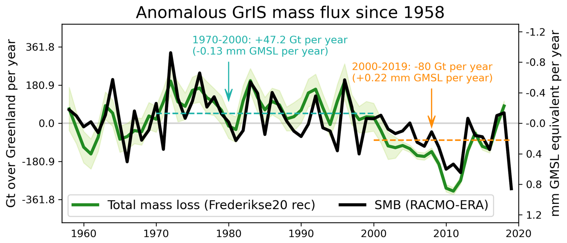
Figure 1 Decadal variability in GrIS' contribution to Global Mean Sea Level (GMSL) is observable and explained by decadal variability in surface mass balance (SMB). The anomalous (long-term mean subtracted) annual GrIS mass loss from the Frederikse et al. (2020a) reconstruction (green) and the anomalous annual GrIS SMB simulated by RACMO with ERA5 reanalysis (RACMO-ERA; black). The thick green lines are the 5000-member ensemble mean values of the Frederikse et al. (2020a) reconstruction, and the shadings are ±1 standard deviation across the 5000 ensemble members.

3.2 Detection and attribution of historical GrIS SMB changes

CESM2-LE with historical forcing (ALL) simulates a decline in SMB that is most apparent after 1990 (Fig. 2a), despite a wide range of internal variability (purple shading) that also covers the interannual variability in RACMO-ERA. According to the D&A framework, the SMB change in RACMO-ERA is detectable and attributable to historical forcing with 99 % confidence (i.e., virtually certain; Fig. 2b). SMB changes can be approximated as precipitation (P) minus runoff (R; Fig. S3, temporal correlation coefficient 0.99, p<0.01, and 1.00, p<0.01, for 10-year running mean time series with 6 eDOF), as sublimation contributes < 10 % of SMB budget (van Kampenhout et al., 2020). The individual time series show that both ALL-forced precipitation and runoff increase (Fig. 2c, e; note that R is inverted). However, this ALL-forced increase in precipitation is not detected in the observation (Fig. 2d), meaning the observed variability of precipitation could just be internal variability (see also van Kampenhout et al. (2020)). On the other hand, the increase in R is detectable and attributable to ALL historical forcing (Fig. 2f; 99 % confidence, virtually certain), agreeing with previous studies that historical GrIS SMB loss is mainly due to warming-driven runoff changes (Noël et al., 2020, 2019; van Kampenhout et al., 2020).

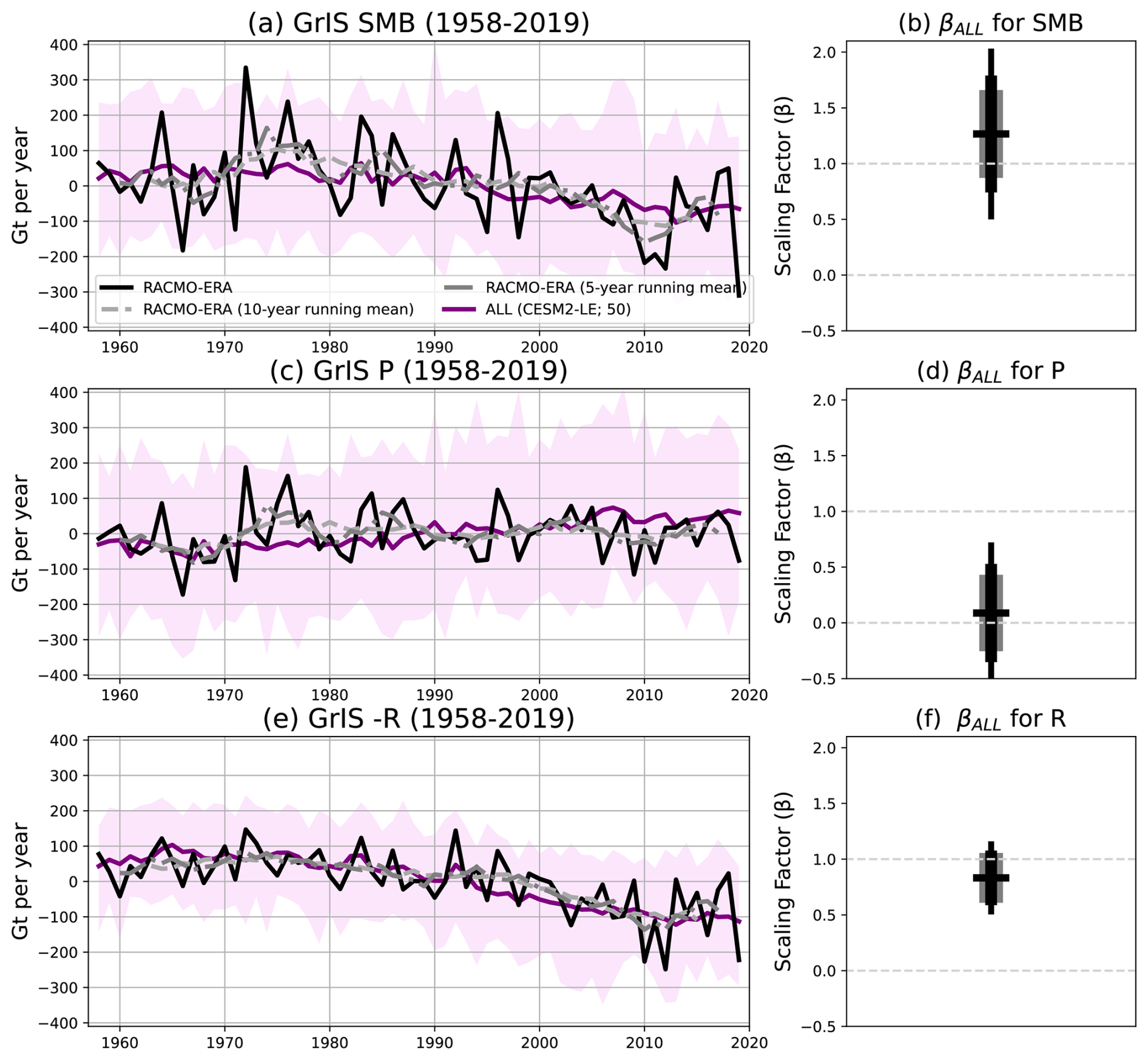
Figure 2 (a, c, e) Time series of annual GrIS SMB, P, -R since 1958 from RACMO-ERA (black; light gray and gray dashed lines are 10-year and 5-year running mean) and ensemble mean of CESM2-LE (purple). The purple shadings are the full range across ensemble members (i.e., maxima to minima). (b, d, f) Univariate scaling factors (β_ALL) of GrIS SMB, P, R. The horizontal line is the mean of the 10 000 posterior samples of β_ALL, and the gray shading/thick black vertical line/thin black vertical line is $\pm \mathrm{1}/\pm \mathrm{1.64}/\pm \mathrm{2.57}$ standard deviation of the 10 000 posterior samples of β_ALL, indicating the 66 %$/$90 %$/$99 % confidence intervals in D&A (likely/very likely/virtually certain based on IPCC guideline). Here, the scaling factor (β_ALL) is derived by the Bayesian Total Least Squares regression with y from RACMO-ERA and x from ensemble mean of CESM2-LE.

The GrIS SMB changes from ALL (Fig. 2a purple solid line) can be approximated as the sum of the changes from GHG and AAER (Fig. S3; temporal correlation coefficient 0.66, p<0.01, for SMB time series from ALL vs. GHG + AAER and 0.93, p<0.01, for 10-year running means with 6 eDOF), with GHG driving a long-term decline in SMB and AAER contributing to an increase before mid-1980 and a slight decrease thereafter (Fig. 3a). Before mid-1980, GHG and AAER basically cancel each other out, while they combine to drive the decline of ALL-forced SMB afterward (Fig. 3a).

A bivariate Bayesian TLS regression is formulated to assess the D&A for these two historical radiative forcings, showing that both GHG (99 % confidence, virtually certain) and AAER (90 % confidence, very likely) contribute to the GrIS SMB changes (Fig. 3b). Interestingly, the posterior distribution of β_GHG has a narrower spread than the posterior distribution of β_AAER, implying a lower S $/$ N in detecting the AAER-forced signal in RACMO-ERA SMB changes. Consistent with Fig. 2, there is no detectable precipitation change due to either GHG or AAER in RACMO-ERA (Fig. 3c, d). However, there is a detectable GrIS runoff change attributed to both GHG and AAER, but both their influences are potentially underestimated (i.e., β_GHG and β_AAER are both significantly larger than 1), and β_AAER also has a wider spread in its posterior distribution than β_GHG for runoff (Fig. 3e, f).

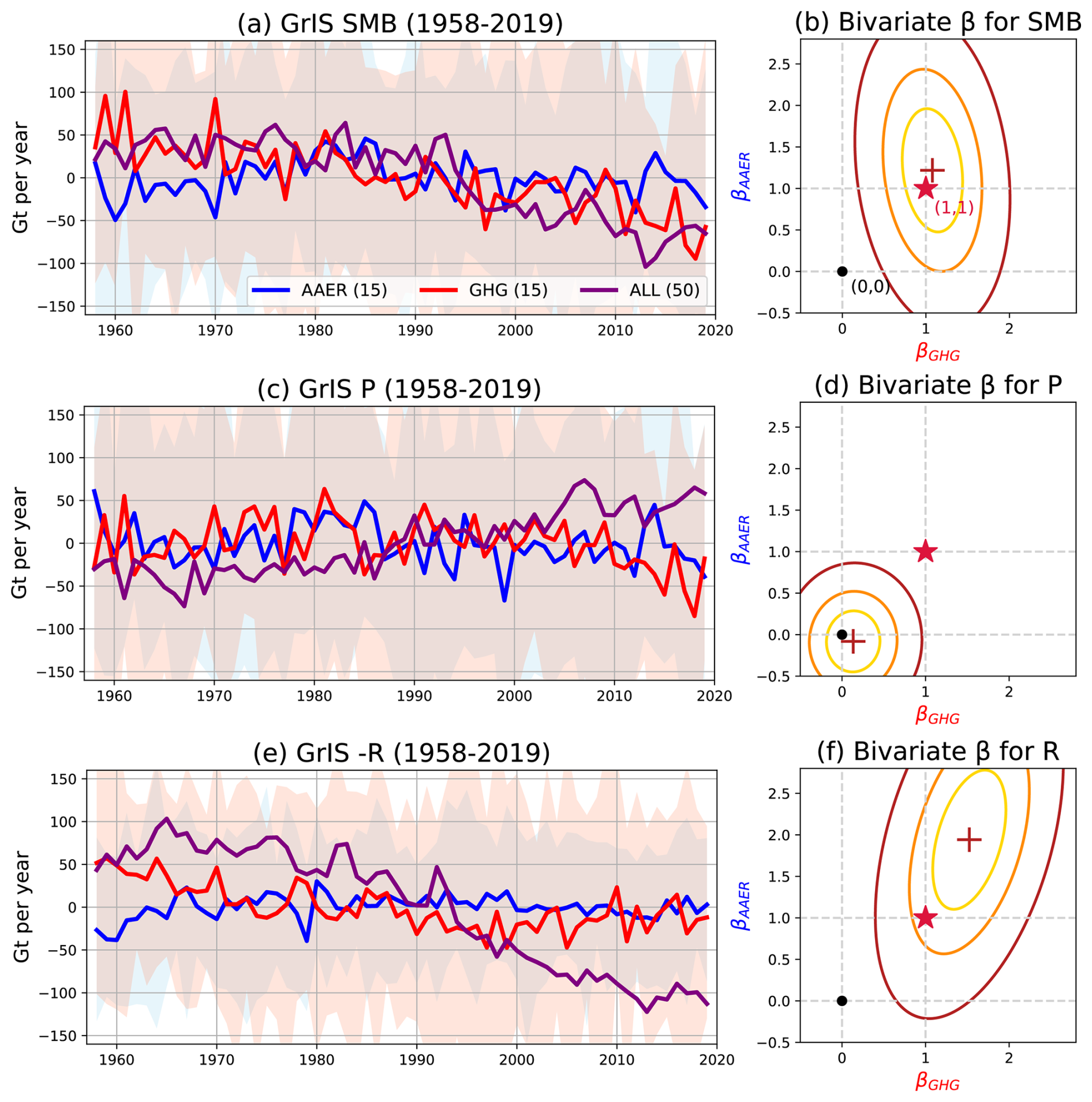
Figure 3 (a, c, e) Time series of annual GrIS SMB, P, -R since 1958 from ensemble mean of CESM2-SFLE greenhouse gases-only simulation (GHG; red), ensemble mean of CESM2-SFLE anthropogenic aerosols-only simulation (AAER; blue), ensemble mean of CESM2-LE ALL simulation (purple as Fig. 2). The red/blue shadings are the full range across ensemble members (i.e., maxima to minima) in GHG/AAER. (b, d, f) Bivariate scaling factors (β_GHG and β_AAER) of GrIS SMB, P, R. The firebrick plus symbol is the mean of the 10 000 posterior samples of β_GHG and β_AAER, and the golden/orange/firebrick confidence ellipses are the 66 %$/$90 %$/$99 % confidence intervals in β_GHG and β_AAER for D&A (likely/very likely/virtually certain based on IPCC guideline). When the confidence ellipse includes the point (1, 1) (shown as the crimson star) and excludes the origin (0, 0) (shown as the black dot), a bivariate attribution to both forcings is established. Here, scaling factors (β_GHG and β_AAER) are derived by the Bayesian Total Least Squares regression with y from RACMO-ERA and x from ensemble mean of AAER and GHG from CESM2-SFLE.

Studies have shown that CESM2 has nonlinear forced responses due to different climate mean states (Simpson et al., 2023) or the non-additive responses to different forcings (Kuo et al., 2025). Therefore, we repeat the bivariate D&A with SMB, precipitation, and runoff from the xAAER and ALL-minus-xAAER simulations to check the robustness of attributing both anthropogenic aerosols and greenhouse gases when using a climate model (CESM2) with reported nonlinear forced responses. Using xAAER and ALL-minus-xAAER to represent GHG and AAER forcing, this analysis yields robust conclusions: GHG and AAER create forced signals in the historical 1958–2019 GrIS SMB through runoff changes, and the attribution to both xAAER and ALL-minus-xAAER is virtually certain (99 % confidence; Fig. S4). Interestingly, the posterior distribution of β_{ALL-minus-xAAER} has a narrower spread for both SMB and runoff compared with the posterior distribution of β_AAER (Figs. S4b and 3b for SMB and Figs. S4f and 3f for runoff), though β_{ALL-minus-xAAER} and β_AAER still have a wider spread than β_xAAER and β_GHG. Additionally, runoff changes are not underestimated in ALL-minus-xAAER and xAAER (Fig. S4f) as they are in GHG and AAER (Fig. 3f), as the means of the posterior bivariate scaling factors are now closer to (1, 1). Thus, there appears to be a state dependence of the attribution to AAER.

Overall, our D&A results indicate that historical GrIS SMB changes are attributable to both GHG and AAER through runoff changes. Despite differences in the scaling factors, these attribution results are robust to the sets of single forcing simulations used (all-but-forcing or forcing-only experimental setups with CESM2). We also point out that there is a lower S $/$ N when attributing GrIS SMB changes and runoff changes to AAER compared with attributing to GHG. This lower S $/$ N when attributing to AAER appears in two ways: (1) underestimated response (usually β_AAER>1 and also >β_GHG) and (2) wider confidence intervals of β_AAER than of β_GHG.

3.3 Mean state temperature affects uncertainty in D&A for AAER

GrIS SMB has a stronger sensitivity to warming than to cooling (Thompson-Munson et al., 2024), and runoff has a nonlinear relationship to temperature change (Trusel et al., 2018). This nonlinear runoff response to temperature is commonly seen in cryospheric variables in response to different mean state temperatures (Gottlieb and Mankin, 2024) with different energy barriers to overcome and/or different positive degree days to start melting and inducing runoff changes (Sherman et al., 2020). Here, we hypothesize that the different temperature sensitivities of runoff in these different simulations might contribute to the lower S $/$ N of the attribution to AAER compared with the attribution to GHG. SMB has a negative temperature sensitivity in RACMO-ERA, ALL, and GHG simulations (Fig. 4a), and all of these simulations demonstrate apparent increases in runoff with warming (Fig. 4b). However, this negative temperature sensitivity is not seen in the AAER simulation (Fig. 4a). There is a nonlinear temperature sensitivity of runoff if the simulations are sorted by their 1958–2019 climatological temperatures (Fig. 4b), explaining the lack of negative temperature sensitivity of SMB in AAER (Fig. 4a). In addition, the mean temperature over the GrIS has a weaker forced response in AAER than in GHG (Fig. S5; also true using ALL-minus-xAAER and xAAER). Together with the weaker temperature sensitivity of SMB in AAER due to the weaker temperature sensitivity of runoff, these two factors lead to a generally lower S $/$ N in attributing SMB changes to AAER than GHG. Precipitation sensitivity to warming is generally positive across simulations (Figure S6), as precipitation usually increases under warming (Held and Soden, 2006). Note that precipitation sensitivity is much higher in the ALL-minus-xAAER simulation than in the AAER simulation (Fig. S6), explaining the slightly more positive SMB sensitivity in ALL-minus-xAAER (Fig. 4a).

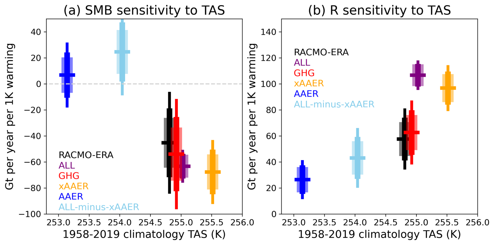
Figure 4 (a) The observed (RACMO-ERA; black) and forced (ALL, GHG, xAAER, AAER, ALL-minus-xAAER; purple, red, orange, blue, light blue respectively) GrIS SMB sensitivity to near-surface temperature during 1958–2019 sorted by the climatological mean near-surface temperature. (b) The observed (RACMO-ERA; black) and forced GrIS R sensitivity to near-surface temperature during 1958–2019 sorted by the climatological mean near-surface temperature. Here, SMB and R sensitivities are derived by the Bayesian Total Least Square regression with SMB or R as y and TAS as x from RACMO, the ensemble mean of CESM2-LE, or the ensemble mean of CESM2-SFLE as appropriate.

This mean state temperature dependent SMB and runoff sensitivity can also explain why the uncertainty ellipse of β using xAAER and ALL-minus-xAAER (Fig. S4) is smaller than the uncertainty ellipse using AAER and GHG (Fig. 3). This is because xAAER and ALL-minus-xAAER simulations both have higher mean state temperatures than GHG and AAER simulations (orange vs. red bars and light blue vs blue bars in Fig. 4). The runoff responses are thus stronger in both the xAAER and ALL-minus-xAAER simulations, and therefore easier to detect; β_xAAER and β_{ALL-minus-xAAER} are both closer to (1, 1) with narrower posterior distributions (Figs. 3f vs. S4f). Although the attribution to AAER is robust across all-but-forcing or forcing-only experimental setups in CESM2, these results demonstrate that mean state temperatures in different simulations can affect their runoff responses and therefore our confidence in attributing SMB changes to that forcing with this D&A framework.

3.4 Atmospheric drivers of forced GrIS runoff changes

What are the mechanisms by which GHG and AAER forcing drive long-term trends and decadal variability in GrIS SMB through runoff changes? Here, we focus on the summer (JJA) temperature and circulation patterns, which are linked to the melting-induced runoff changes (Sherman et al., 2020; Hanna et al., 2014; Tedesco and Fettweis, 2020). The trend map for 1958–2019 from ERA5 shows overall JJA polar warming and increasing Z₅₀₀ over Greenland (Fig. 5a), consistent with the Greenland Block Index (GBI) time series (Fig. S7a). The correlation between annual GrIS runoff and JJA near-surface temperature and JJA Z₅₀₀ from ERA5 is positive, i.e., a Greenland blocking pattern (Fig. 5e). Greenland blocking provides more cloudless days and subsidence-induced warming (Sherman et al., 2020), as well as warm air advection towards Western Greenland (Hanna et al., 2014; Tedesco and Fettweis, 2020) due to the anti-cyclone over Greenland. The correlation pattern in ERA5 remains consistent even after detrending and temporal smoothing (Fig. S8). Thus, the long-term linear trend has little impact on the correlation pattern seen in ERA5.

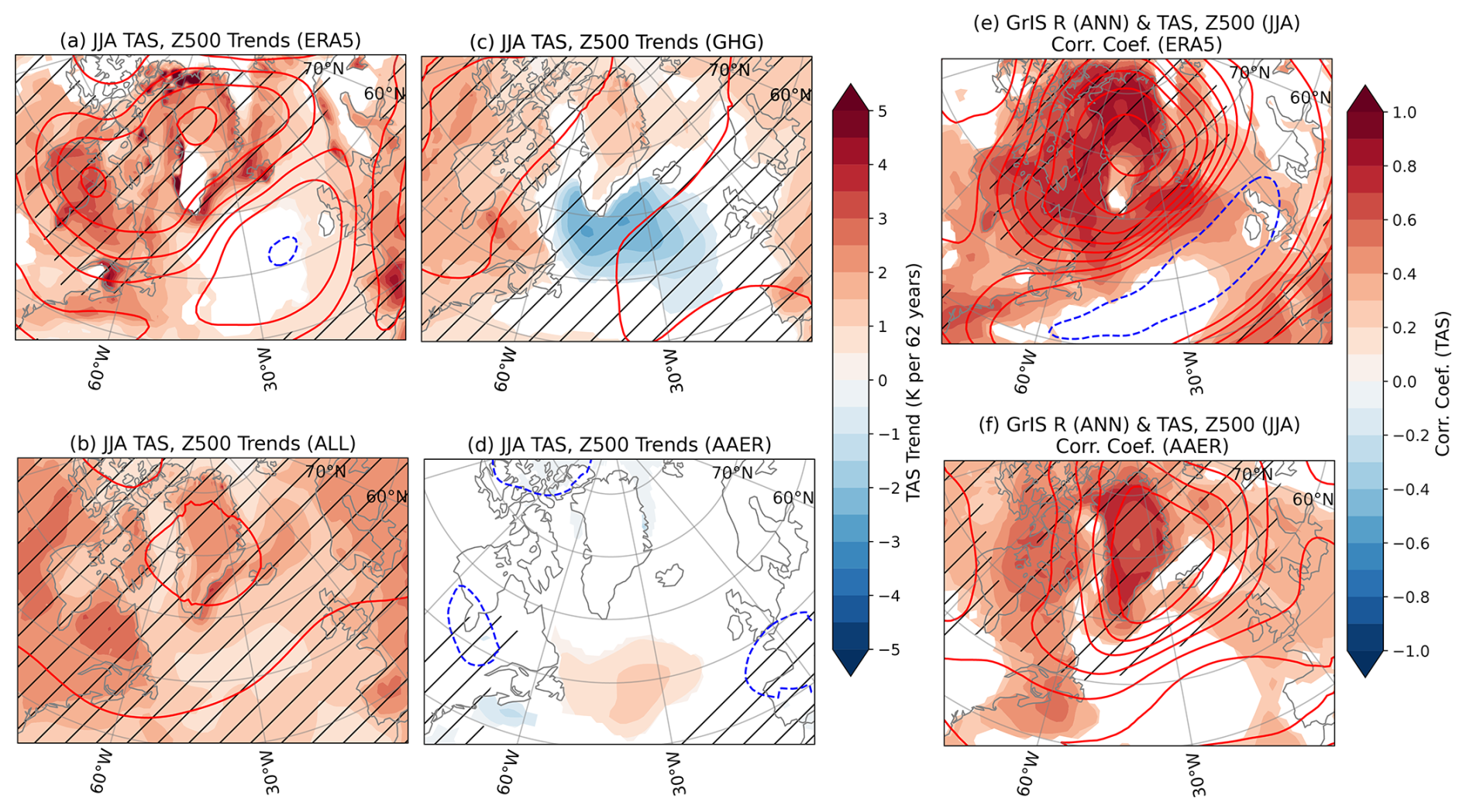
Figure 5 Trend maps of 500 hPa geopotential height (Z₅₀₀; contours) and near-surface air temperature (TAS; shading) during 1958–2019 in (a) ERA5 reanalysis, (b) ensemble mean of all forcings CESM2-LE simulations (50; ALL), (c) ensemble mean of GHG-only simulations (15; GHG), and (d) ensemble mean of AAER-only simulations (15; AAER). Grid cells with insignificant TAS trends are masked out (95 % confidence for ERA5, and ensemble mean trend over 1 standard deviation across all trends in the ensemble for climate model simulations). Grid cells with significant Z₅₀₀ trends are hatched (95 % confidence for ERA5 and ensemble mean trend over 1 standard deviation across all possible trends in the ensemble for climate model simulations). Z₅₀₀ contours start from ±10 (m per 62 years) with contour spacing of 10 (m per 62 years). (e–f) Correlation map of GrIS R with Z₅₀₀ (contours) and TAS (shading) during 1958–2019 in (e) ERA5 reanalysis and (f) 15-member mean AAER. Insignificant TAS correlations are masked out and significant Z₅₀₀ correlations are hatched (95 % confidence). Contours start from 0.1 with contour spacing of 0.1. The significance level of the correlation coefficients is based on a t-test with the degrees of freedom corresponding to the length of data (1958–2019, 62 years).

JJA near-surface warming and Z₅₀₀ increasing trends over the North Atlantic sector are visible in both ALL (Fig. 5b) and GHG (Fig. 5c). Though the ALL-forced Z₅₀₀ trend is weaker than the observed Z₅₀₀ trend (consistent with GBI in Fig. S7 and Delhasse et al. (2021)), the observed trend is within the range of possible trends from the 50-member ALL ensemble. The forced temperature and Z₅₀₀ trends from ALL and GHG are overall alike, confirming that GHG contributes to the long-term linear trend seen in these atmospheric variables related to GrIS runoff changes. However, in GHG, the Atlantic Meridional Overturning Circulation (AMOC) declines more rapidly than in ALL, as it lacks the offsetting North Atlantic cooling from AAER (Fig. 9 in Simpson et al. (2023)), leading to cooling in the Subpolar Gyre. Additionally, ALL-forced JJA Z₅₀₀ increases with a blocking-like structure over Greenland, while GHG-forced JJA Z₅₀₀ increases more uniformly (Fig. 5b vs. c contour). A cooling of the Subpolar Gyre in GHG simulation and a stronger subsidence trend in ALL together lead to less warming in GHG than in ALL (Fig. 5b vs. c).

In addition, the Subpolar Gyre cooling correlates with a more positive NAO (Fan et al., 2023). This implies a less negative NAO/reduced Greenland blocking as a result of this air-sea coupled feedback over the Subpolar Gyre, which may explain why GHG-forced runoff (Fig. 3e) and GBI (Fig. S7b) plateaus after 2000 when the Subpolar Gyre cooling intensifies. This is also supported by the significant correlations of an emerging Greenland blocking pattern in GHG (Fig. S9a) that differs from its uniform warming and Z₅₀₀ trends (Fig. 5c), regardless of whether linear trends in GHG are removed or not (Fig. S9a vs. b). Although beyond the scope of this study, idealized experiments to distinguish the circulation changes originating from direct GHG radiative forcing versus from GHG-induced Subpolar Gyre SSTs would help advance understanding of the role of atmospheric circulation changes in GrIS mass loss.

AAER, on the other hand, contributes almost nothing to this long-term trend pattern (Fig. 5a vs. d). These trend maps imply that the detected signal from AAER during 1958–2019 (Fig. 3b, f) does not arise through the long-term linear trend but through forced decadal variability undergoing phase changes during this time period. We compare maps of the correlation from ERA5 (Fig. 5e) and from the ensemble mean of AAER during 1958–2019 (Fig. 5f). The AAER-based correlation map shows a pattern that is distinct from its long-term trend (Fig. 5f vs. d); instead, the correlation map shows a pattern more similar to the ERA5-based correlation map (Fig. 5e vs. f). Both ERA5 and AAER have positive correlations between GrIS runoff and near-surface temperature and Z₅₀₀. Figure 5f confirms a similar correlation pattern due to AAER, supporting an AAER-forced change in the variability of circulation, imprinted onto a pattern that reinforces Greenland blocking, consistent with Maddison et al. (2024).

4 Discussion and Conclusion

In this paper, we formulate a D&A analysis with CESM2-LE and CESM2-SFLE to investigate 1958–2019 GrIS SMB change and show that the historical SMB change is attributable not only to GHG but also to AAER. To our knowledge, this is the first manuscript demonstrating that parts of the historical GrIS SMB change are attributable to AAER. Specifically, GHG drives the long-term SMB decline, while AAER contributes to the decadal variability of SMB, consistent with a growing literature on how AAER induces decadal variations to other aspects of historical North Atlantic climate change (Scaife and Smith, 2018).

To understand the mechanisms of forced SMB change, we consider two perspectives. First, from a mass balance perspective, we demonstrate that the historical forced SMB changes in a ERA5 reanalysis-based RACMO simulation are mainly driven by runoff changes, irrespective of the underlying forcing (GHG or AAER). Second, we investigate the atmospheric pathways by which these forcings affect runoff, demonstrating that the GHG-forced runoff change is mainly driven by long-term warming and the AAER-driven runoff change relates to atmospheric circulation variability of Greenland blocking on decadal time scales (Sherman et al., 2020; Brils et al., 2023; Hanna et al., 2022). These results highlight that different climate forcings can drive SMB changes through different physical mechanisms, with different spatial patterns and time scales (i.e., long-term trend vs decadal variability).

Attribution of regional climate change to AAER often has a low S $/$ N compared to GHG attribution (e.g., Marvel et al. (2019)) and our study confirms this tendency. In the case of attributing GrIS SMB, this is due to the temperature sensitivity of runoff being weaker in AAER than GHG, as the sensitivity strongly depends on mean state temperatures in each simulation. We compare the sets of forcing-only (GHG and AAER) and all-but-forcing (xAAER and ALL-minus-xAAER) CESM2 experiments, where we show robust attribution of historical GrIS SMB changes to both GHG and AAER through runoff changes. The mean state temperature dependency of runoff response can also explain the difference of S $/$ N in the forcing-only and all-but-forcing sets, as their mean state temperatures are different. Although we show that both AAER and GHG contribute to the historical GrIS SMB changes, such a mean state temperature dependence of the forced SMB response implies a potential bias in the current D&A framework – certain forcings, such as GHG, can individually create a mean state with a stronger response that is more likely to be attributed. Future work will need to develop D&A methods that can systematically account for mean state temperature dependency in climate responses.

CESM2 and RACMO simulate reasonable SMB and water budgets (Noël et al., 2018; van Kampenhout et al., 2020); however, both are subject to model structural uncertainty. The model structural uncertainty accounts for most of the uncertainty in SMB future projections (Holube et al., 2022). The snow parameterization uncertainty contributes to part of the high model structural uncertainty in SMB but does not serve as the main contributor (Holube et al., 2022). Instead, it comes from atmospheric variables, as GrIS precipitation, temperature, and Z₅₀₀ all show high model structural uncertainties in their future projections (Zhang et al., 2024). One motivation to conduct D&A with Bayesian regression, instead of a deterministic regression, is to account for the uncertainty in estimates of forced responses (from CESM2) and of observations (from RACMO). Still, we acknowledge the caveat that this study does not fully sample model structural uncertainty. Future work to extend D&A with more climate models could enhance the robustness of the results presented here. Such efforts could also support the development of observational constraints on SMB projections, for example, based on the temperature sensitivity presented here.

On top of the different runoff responses due to the mean state temperature dependence, we note that historical aerosol emissions used in CMIP6 simulations have large uncertainties, especially pre-1980 (Mahowald et al., 2024). Beyond the scope of this paper, future works should thus explore the impacts of aerosol emissions and forcing uncertainties on D&A of GrIS SMB changes.

The mean state temperature dependency of runoff found in our study implies that GrIS SMB changes might accelerate in the future, especially as we expect continued increases in greenhouse gases with simultaneous reductions in anthropogenic aerosols (Samset et al., 2018; Persad et al., 2022). Thus, under stronger warming in these future projections, further growth in the contribution of GrIS SMB reduction to GMSL rise is foreseeable.