Ensemble-based data assimilation improves hyperresolution snowpack simulations in forests

Snowpack dynamics play a key role in controlling hydrological and ecological processes at various scales, but snow monitoring remains challenging. Data assimilation techniques are emerging as promising tools to improve uncertain snowpack simulations by fusing state-of-the-art numerical models with information rich, but noisy observations. However, the occlusion of the ground below the forest canopy limits the retrieval of snowpack information from remote sensing tools. Remote sensing observations in these environments are spatially incomplete, impeding the implementation of fully distributed data assimilation techniques. Here we propose different experiments to propagate the information obtained in forest clearings, where it is possible to retrieve observations, towards the sub-canopy, where the point of view of remote sensors is occluded. The experiments were conducted in forests within Sagehen Creek watershed (California, USA), by updating simulations conducted with the Flexible Snow Model (FSM2) using airborne lidar snow data using the Multiple Snow data Assimilation system (MuSA). The successful experiments improved the reference simulations significantly both in terms of validation metrics (correlation coefficient from R=0.1 to R=0.8 on average) and spatial patterns. Data assimilation configurations using geographical distances and space of topographical dimensions, improved the reference run. However, those creating a space of synthetic coordinates by combining the spatiotemporal data assimilation with a principal components analysis did not show any improvement, even degrading some validation metrics. Future data assimilation initiatives would benefit from building specific localization functions that are able to model the spatial snowpack relationships at different resolutions.

1 Introduction

The seasonal snowpack is a crucial component in various ecological and hydrological processes in mountain areas and cold regions (Han et al., 2024; Slatyer et al., 2022), covering over 47 million square kilometers of the northern hemisphere (Robinson and Frei, 2000) and 45 % of global mountain areas (Gascoin et al., 2024),. It has significant implications for both the economy and ecology of these areas, as well as for downstream regions (Barnett et al., 2005; Qin et al., 2020; Sturm et al., 2017). However, accurately estimating the spatiotemporal dynamics of the snowpack, in particular the snow water equivalent (SWE), remains a challenging and unresolved issue (Tsang et al., 2022). These difficulties are only increased in forested terrain, due to the complex relationships between snowpack and canopy cover (Mazzotti et al., 2020a).

The overlapping area between the snowpack and forested areas is estimated in at least 19 % of the terrain in the northern hemisphere, only accounting for the boreal forest (Rutter et al., 2009). This estimation can only be higher considering the overlapping area in alpine forests. Snow beneath the canopy behaves differently than in open terrain (Dickerson-Lange et al., 2023; Safa et al., 2021; Varhola et al., 2010). The intercepted snow will either sublimate, drip as liquid water or unload as snow (Lundquist et al., 2021). In addition, the canopy cover changes the net radiation available to melt the snowpack, both by shading the snow surface and increasing the incoming longwave radiation (Lundquist et al., 2013). Generally, this leads to increased ablation under the canopy in warmer environments from longwave radiation compared to colder environments where shading from solar radiation causes less ablation under canopy (Lundquist et al., 2013). This relationship leads to differences between under canopy and open clearing snowpack in most environments (Dickerson-Lange et al., 2017) that are challenging to observe across complex terrain (Safa et al., 2021).

Direct observations of the snowpack under the forest are rare and challenging to obtain (Kinar and Pomeroy, 2015). Remote sensing techniques are well established as snow cover monitoring tools (Gascoin et al., 2024). Due to different remote sensing initiatives, it is possible to monitor the dynamics of the snowpack even at continental scales at frequencies approaching real time. Unfortunately, most of these retrievals are limited to observations in open terrain or clearings in forested areas, being limited either spatially or temporally. One partial solution to observing snow under the canopy is with airborne lidar systems that can partially penetrate the canopy and retrieve the snow depth. Recent work has processed lidar point clouds to resolve under canopy snowpack and validated the results against field observations (Kostadinov et al., 2019; Safa et al., 2021; Piske et al., 2025).

Numerical modeling of the snowpack allows simulating the complete state of the snowpack, including the SWE, at any spatiotemporal resolutions. Modern snowpack models of increasing complexity even represent the horizontal transport of the snow caused by wind and avalanches, and the interactions with forests (Mazzotti et al., 2020b; Vionnet et al., 2021). However, numerical models often rely on adjustable parameters to represent different physical processes, whose transferability between different areas and model resolutions is usually complex, leading to uncertain simulations (Essery et al., 2013). In addition, these models rely on high resolution meteorological forcings, that are very challenging to generate and constrain, in part due to the lack of dense in situ observations. The computational cost of regional atmospheric models increases significantly with finer resolution, with the current state of the art at the kilometer scale (Rasmussen et al., 2023). A partial, and very widespread, solution to this problem is to use simplified downscaling models that rely on different assumptions and/or empirical approximations to generate high resolution meteorological forcing fields (Fiddes and Gruber, 2014; Liston and Elder, 2006; Reynolds et al., 2023). Despite their simplicity, these more heuristic approaches may lead to a performance comparable with dynamically downscaled meteorological products (Alonso-González et al., 2023b; Gutmann et al., 2012; Kruyt et al., 2022). Nonetheless, any (often considerable) remaining uncertainty in the forcing will, together with the uncertainty in the snow model structure and parameters, be propagated to the snowpack simulations, typically leading to simulations that differ significantly from reality (Krinner et al., 2018; Raleigh et al., 2015).

Data assimilation (DA) is the exercise of merging noisy observations with uncertain numerical models to exploit the strengths of both worlds (Evensen et al., 2022). Thanks to DA, it is possible to constrain model uncertainty using partial information from snowpack observations (Largeron et al., 2020). Using DA, it is possible to infer uncertain parameters to improve the simulations so as to better match the observations, providing an estimation of the model uncertainty. However, snow DA is still rarely used in forested areas due to the lack of reliable remote sensing observations of the snowpack under the canopy.

Canopy cover impedes the direct observation of the snowpack from space or airborne sensors, which collaterally hampers the use of DA, and may even degrade simulation outputs if implemented in its simplest form (Yatheendradas et al., 2012). This is probably the reason that the majority of snow DA experiments have been limited to arctic or alpine areas above the treeline, with only some experiments approaching specifically the topic of snow DA in forested areas. Smyth et al. (2022) tested the potential of a particle filter DA algorithm to improve snowpack simulations generated by the Flexible Snow Model (FSM2, Essery et al., 2025) in the presence of observations beneath the canopy. The results show that simulations can be improved by assimilating data in snow models that consider canopy interactions. However, the question of how to improve simulations of the snowpack in case of a total occlusion of the snow view in certain regions of the simulation domain (i.e. lack of local observations) remains unanswered. Pflug et al. (2024) proposed a simplified three dimensional DA scheme to update the SWE state variable at unobserved locations from remote observations in forest gaps and tested their approach with a synthetic observing system simulation experiment (OSSE). Due to its simplicity, their heuristic procedure succeeded in performing a promising synthetic assimilation experiment over a very large area of North America at an affordable computational cost. Cho et al. (2023) assimilated spatially coarse airborne gamma ray based SWE retrievals in forested environments, using a three-dimensional EnKF. These recent works lay the foundations of snow data assimilation in forests, with great potential to (i) improve snowpack simulations in forested watersheds, (ii) better understand snow-forest processes, and (iii) identify shortcomings in snow-forest model parameterizations. However, these previous works are based on necessarily simplified approximations to limit the computational cost, synthetic experiments or very coarse resolutions unable to capture the spatial variability present in montane forests (Safa et al., 2021; Tennant et al., 2017). The emergence of new technologies that allow the acquisition of snowpack observations at high and hyper resolutions (Gascoin et al., 2024), make it necessary to adapt classical DA techniques to maximize the value of the available information.

The interactions between the canopy and the snowpack behavior pose challenges for inferring the snow mass beneath the canopy directly from nearby observed locations in forest clearings, preventing simple interpolation techniques (Dharmadasa et al., 2024) or DA techniques designed to update the model states directly from the information obtained in nearby cells to work efficiently in this context (Pflug et al., 2024). It is necessary to explore how the available information can be transferred from the observations in forest clearings to beneath the canopy, where observations are typically either missing or highly uncertain. In this work, we test a recently developed spatio-temporal snow DA methodology (Alonso-González et al., 2023b), specifically designed to update distributed snowpack simulations from spatially incomplete observations such as in a forest environment where the information from remote sensors is mostly available in forest clearings. We combine that information with a unique post-processed lidar dataset that resolves the under-canopy snowpack explicitly (Kostadinov et al., 2019; Piske et al., 2025) to validate the model. The objective of this work is (i) to explore the potential of lidar-derived real observations to update distributed snowpack simulations at hyperresolution (10 m) scales in forest environments, and (ii) to test different spatiotemporal DA configurations for estimating snow under the canopy when only observations in forest gaps are available. Here we propose different spatio-temporal DA configurations to propagate information under the canopy where the observations are often not available.

2 Data and Methods

2.1 Observed snow depth maps, vegetation parameters and meteorological forcing

The experiments proposed in this work were developed in the Sagehen Creek forest (California, USA, Fig. 1). The observations consist of one airborne LiDAR derived snow depth map collected by the National Center for Airborne Laser Mapping on 21 March 2022 (Piske, 2022) and a snow-off flight (Graup, 2021). From all the available areas, we have selected a domain of 2×2 km that maximizes canopy heterogeneity and the observed snowpack data that are incomplete due to dense canopy cover. The Sagehen Creek site was used to develop and test a new method of under canopy snow depth detection from airborne lidar (Kostadinov et al., 2019) that resolves a considerable amount of snow information beneath the canopy (Fig. 1). We use an improved method, as compared to Kostadinov et al. (2019), to extract vegetation from the snow surface described in Piske et al. (2025) that better resolves low vegetation from the snow surface using the lidar point cloud. Based on nearby SNOTEL at a similar elevation (SNOTEL Site: 539, Independence Camp, https://wcc.sc.egov.usda.gov/nwcc/site?sitenum=539, last access: 11 November 2024), the SWE was 43 cm on 21 March when lidar was collected compared to a maximum annual SWE of 48 cm on 9 March, 2022. The native spatial resolution of the lidar dataset was 1 m which was resampled to 10 m for use in the DA analysis. The error variance of the observations was assumed to be σ²=0.01 m² at 10 m resolution based on previous airborne LiDAR snow experiences that reported similar error metrics (Currier et al., 2019; Harpold et al., 2014; Mazzotti et al., 2019; Painter et al., 2016). Future initiatives may benefit from more sophisticated error models. In addition to the snow depth observations, different vegetation parameters were computed from the three-dimensional lidar data, including vegetation height, the Vegetation area index and the in forest sky view factor based on methods described in Broxton et al. (2015) and Broxton et al. (2021). This dataset was segmented into grid cells in forest clearings (to be assimilated) and canopy-covered cells (to be used as independent validation) based on this vegetation information. The meteorological forcing was generated using MicroMet (Liston and Elder, 2006) forced by the ERA5 atmospheric reanalysis (Hersbach, 2000). The meteorological fields were downscaled to the same geometry of the observations using a LiDAR based digital elevation model (Sourp et al., 2025). The precipitation partitioning was estimated using the psychrometric parameterization scheme proposed by Harder and Pomeroy (2013).

Figure 1 (a) Localization map, (b) Digital elevation model, (c) vegetation height and (d) available observations (with its segmentation between canopy covered data used for validation or forest gaps to be assimilated). The red transect in the digital elevation map indicates the location of the profile used later for validation.

2.1.1 Data assimilation and computational setup

All DA experiments presented in this work were developed using the Multiple Snow data Assimilation (MuSA) system (Alonso-González et al., 2022). MuSA is an open-source DA toolbox designed primarily as a python wrapper around FSM2, but now providing support for other numerical models as well while not necessarily being limited to snowpack models. MuSA provides support to different DA algorithms, and simplifies the implementation of new ones thanks to its modular design. In this work, the FSM2 model was chosen due to its already coupled canopy module that required only minimal modifications of the original MuSA code to be activated. MuSA, and therefore FSM2, was forced by the MicroMet outputs, and provided with the lidar-derived vegetation parameter maps. The most complex FSM2 parameterisation was selected, based on previous experience. In the case of canopy parameterisation, this includes a two layer canopy model with nonlinear snow interception, snow unloading dependent on wind or temperature and two-stream approximation canopy radiative transfer. In any case, the methods presented here are independent of the numerical model and forcing used, so they are transferable to different snow data assimilation initiatives. It should be noted that although in this work we focus on the MuSA snow depth outputs (as this is what we can validate) posterior simulations include the full state vector of FSM2, including SWE.

The spatio-temporal DA scheme is described in Alonso-González et al. (2023b), and therefore we only briefly introduce some key points here, its configuration, and the new modifications implemented to improve its performance for the new problem at hand. We only infer meteorological correction parameters and not model states, leading to physically consistent (in terms of FSM2) simulations of the modeled snow state across the snow season. As mentioned above, snowpack in the forest gaps shows a different behavior than beneath the trees (Varhola et al., 2010), so trying to infer canopy-occluded states directly from the information we can obtain in the gaps could also introduce artifacts in the simulations. Crucially the forcing perturbations will also be modified by the canopy scheme in FSM2, so even if the above canopy forcing is constrained to be similar for neighboring cells the forcing that the below canopy snowpack experiences will be different due to model physics.

As the first step in our workflow, we generated an ensemble of 100 FSM2 simulations by randomly drawing stationary (i.e. constant across the water year) spatially correlated prior parameters to perturb the meteorological forcing, particularly the precipitation and 2 m air temperature fields. The choice of perturbing only precipitation and temperature was motivated by previous successful experiments with a similar setup, albeit in non-forested environments (Alonso-González et al., 2023a; Alonso-González et al., 2022). Herein, the prior probability distributions that we sampled using a random number generator were: a normal (additive parameter) for the temperature bias and lognormal (multiplicative parameter) for the precipitation scaling. These prior distributions were defined by: its mean (μ=0) and standard deviation (σ=1) in the case of the temperature and by the mean and standard deviation (μ=0, σ=0.4) of the underlying normal distribution in the case of the precipitation. The latter results in log-normally distributed prior multiplicative precipitation scaling parameters in the physical space whose median is 1. The objective of the algorithm is to update these parameters by assimilating observations to directly correct the temperature and precipitation fields and indirectly update the corresponding snowpack states.

For this purpose we have used a deterministic ensemble Kalman filter (DEnKF)-based algorithm in iterative smoother mode, namely the Deterministic Ensemble Smoother (DES, Sakov and Oke, 2008) with multiple data assimilation (DES-MDA, Emerick, 2018). In this DES-MDA scheme, the update proceeds in two steps for each grid cell $i=\mathrm{1},\mathrm{\dots },N_{\mathrm{g}}$ and $\mathrm{\ell }=\mathrm{0},\mathrm{\dots },(N_a-\mathrm{1})$ MDA iteration. Firstly, the N_p×1 updated ensemble mean parameter column vector ${\stackrel{\mathrm{‾}}{\mathit{\theta }}}_{\mathrm{\ell }+\mathrm{1}}^{\left(i\right)}$ is obtained using a Kalman analysis equation of the form

$$\begin{array}{}\text{(1)}& {\stackrel{\mathrm{‾}}{\mathit{\theta }}}_{\mathrm{\ell }+\mathrm{1}}^{\left(i\right)}={\stackrel{\mathrm{‾}}{\mathit{\theta }}}_{\mathrm{\ell }}^{\left(i\right)}+{\mathbf{K}}_{\mathrm{\ell }}^{\left(i\right)}\left[{\mathit{y}}^{\left(i\right)}-{\stackrel{\mathrm{‾}}{\mathit{y}}}_{\mathrm{\ell }}^{\left(i\right)}\right]\end{array}$$

where ${\stackrel{\mathrm{‾}}{\mathit{\theta }}}_{\mathrm{\ell }}^{\left(i\right)}$ is the N_p×1 ensemble mean parameter column vector from the current (prior for ℓ=0) iteration, the $N_p\times N_{\mathrm{o}}^{\left(i\right)}$ matrix ${\mathbf{K}}_{\mathrm{\ell }}^{\left(i\right)}$ is a localized and inflated ensemble Kalman gain computed using ensemble covariances and the observation error covariance, y⁽ⁱ⁾ is the $N_{\mathrm{o}}^{\left(i\right)}\times \mathrm{1}$ local observation vector containing available local observations that are within a yet to be defined distance-based neighborhood d>2c (see the GC function below) of grid cell i, and the $N_{\mathrm{o}}^{\left(i\right)}\times \mathrm{1}$ vector ${\stackrel{\mathrm{‾}}{\mathit{y}}}_{\mathrm{\ell }}^{\left(i\right)}$ contains the corresponding local ensemble mean predicted (i.e. modeled) observations from the last iteration obtained at neighboring grid cells. We refer to Alonso-González et al. (2023a) for the full form of the ensemble Kalman gain matrix in particular and a more detailed overview of the implementation of spatio-temporal DA using the DES-MDA in MuSA in general. Secondly, the N_p×N_e matrix ${\mathbf{\Theta }}_{\mathrm{\ell }+\mathrm{1}}^{(i{)}^{\prime }}$ containing the updated ensemble of parameter vector anomalies (from the mean) is obtained using a modified Kalman analysis equation of the form

$$\begin{array}{}\text{(2)}& {\mathbf{\Theta }}_{\mathrm{\ell }+\mathrm{1}}^{(i{)}^{\prime }}={\mathbf{\Theta }}_{\mathrm{\ell }}^{(i{)}^{\prime }}-\mathrm{0.5}{\mathbf{K}}_{\mathrm{\ell }}^{\left(i\right)}\left[{\mathit{y}}^{\left(i\right)}{\mathbf{1}}_{N_{\mathrm{o}}^{\left(i\right)}}^{\mathrm{T}}-{\widehat{\mathbf{Y}}}_{\mathrm{\ell }}^{\left(i\right)}\right]\end{array}$$

where ${\mathbf{\Theta }}_{\mathrm{\ell }}^{(i{)}^{\prime }}$ is the N_p×N_e matrix containing the ensemble of parameter vector anomalies from the current iteration, ${\mathbf{1}}_{N_{\mathrm{o}}^{\left(i\right)}}^{\mathrm{T}}$ is a $\mathrm{1}\times N_{\mathrm{o}}^{\left(i\right)}$ row vector of ones, and ${\widehat{\mathbf{Y}}}_{\mathrm{\ell }}^{\left(i\right)}$ is the $N_{\mathrm{o}}^{\left(i\right)}\times N_e$ matrix of predicted observations from the current iteration. Once the mean and anomaly update steps have been carried out, the N_p×N_e matrix ${\mathbf{\Theta }}_{\mathrm{\ell }+\mathrm{1}}^{\left(i\right)}$ (without the prime) containing the updated ensemble of parameter vectors is obtained through the matrix sum

$$\begin{array}{}\text{(3)}& {\mathbf{\Theta }}_{\mathrm{\ell }+\mathrm{1}}^{\left(i\right)}={\stackrel{\mathrm{‾}}{\mathit{\theta }}}_{\mathrm{\ell }+\mathrm{1}}^{\left(i\right)}{\mathbf{1}}_{N_p}^{\mathrm{T}}+{\mathbf{\Theta }}_{\mathrm{\ell }+\mathrm{1}}^{(i{)}^{\prime }}\end{array}$$

where ${\mathbf{1}}_{N_p}^{\mathrm{T}}$ is a 1×N_p row vector of ones. Unlike the classic stochastic (perturbed observation) ensemble Kalman scheme, this deterministic ensemble Kalman scheme is less overconfident thanks to built-in model covariance inflation and also avoids the need to factorize the observation error covariance that can be costly in spatio-temporal problems (Emerick, 2018). In the loop over iterations above we implicitly rerun the forward model, FSM2 in this case, with the updated parameter values to generate an updated ensemble of hidden snowpack states including the predicted snow depth observations to be assimilated.

The Gaussian assumptions inherent in this ensemble Kalman method make it more robust against ensemble collapse (where a single member carries all the posterior probability) than particle methods which are more widely used for snow DA (Alonso-González et al., 2022). In particular, we have used an iterative version of DES, that performs the update of the parameters in multiple data assimilation (MDA) steps, creating the DES-MDA used here (Emerick, 2018). The MDA is a form of likelihood tempering (Murphy, 2023) that helps relax the undesirable effects of the linear assumption inherent to EnKF based algorithms. In nonlinear DA problems such as the one tackled here, previous work has shown that these MDA iterations lead to significant improvement of the results compared with non-iterative versions of the algorithm (Aalstad et al., 2018; Alonso-González et al., 2022). In this work, based on previous studies (see Alonso-González et al., 2022 and references therein), the number of iterations was fixed to 4. To accommodate the Gaussian assumption, we employed analytical Gaussian anamorphosis (Bertino et al., 2003) to log transform the precipitation parameter distribution to a normal distribution and perform the update in Gaussian space. After the update, the parameters are mapped back to the model space using the exponential function before generating the new ensembles.

The spatial propagation of information may happen through two main mechanisms in the DES-MDA: observation error correlations or prior correlations (van Leeuwen, 2019). Since observation error correlations are more challenging to specify and arguably less general than prior correlations, we will focus only on the latter. A key component of the scheme is to draw random prior parameters for each cell that are correlated with other cells in the domain, reflecting similarities among different regions of the simulation domain. In the general DA literature, this is typically done by computing the pairwise geographic (Euclidean) distance to map the proximity of the cells. The pairwise distance matrix is then used to generate a covariance matrix. In this work we have used the 5th-order piecewise rational function proposed by Gaspari and Cohn (GC) (Gaspari and Cohn, 1999), as is often done in DA to generate and localize the covariance matrix. The GC localization function depends on an important hyperparameter, the correlation length scale, that in practice controls how far information can be transferred spatially. Crucially, this length scale will affect both the posterior results and the computational cost since a larger length scale results in a greater number of neighbors with non-zero correlation. The GC function defines a distance-based correlation as follows

$$\begin{array}{}\text{(4)}& \mathit{\rho }\left(d,c\right)=\left\{\begin{array}{l}-\frac{\mathrm{1}}{\mathrm{4}}{\left(\frac{d}{c}\right)}^{\mathrm{5}}+\frac{\mathrm{1}}{\mathrm{2}}{\left(\frac{d}{c}\right)}^{\mathrm{4}}+\frac{\mathrm{5}}{\mathrm{8}}{\left(\frac{d}{c}\right)}^{\mathrm{3}}-\frac{\mathrm{5}}{\mathrm{3}}{\left(\frac{d}{c}\right)}^{\mathrm{2}}+\mathrm{1},\\ \text{for }\mathrm{0}\le \left(\frac{d}{c}\right)\le \mathrm{1},\\ \frac{\mathrm{1}}{\mathrm{12}}{\left(\frac{d}{c}\right)}^{\mathrm{5}}-\frac{\mathrm{1}}{\mathrm{2}}{\left(\frac{d}{c}\right)}^{\mathrm{4}}+\frac{\mathrm{5}}{\mathrm{8}}{\left(\frac{d}{c}\right)}^{\mathrm{3}}+\frac{\mathrm{5}}{\mathrm{3}}{\left(\frac{d}{c}\right)}^{\mathrm{2}}-\mathrm{5}\left(\frac{d}{c}\right)\\ +\mathrm{4}-\frac{\mathrm{2}}{\mathrm{3}}{\left(\frac{d}{c}\right)}^{-\mathrm{1}},\text{for }\mathrm{1}\le \frac{d}{c}\le \mathrm{2},\\ \mathrm{0},\text{for }\frac{d}{c}>\mathrm{2}.\end{array}\right.\end{array}$$

where, d is the pairwise distance between cells and c is the correlation length scale. This function is used for localization, with two important roles: first, it reduces spurious long range correlations that arise due to the limited size of the ensemble (Morzfeld and Hodyss, 2023), and second, to save considerable computational costs since relatively distant locations can be ignored when updating a particular cell. Note that without localization, the spatio-temporal DA problem would essentially be intractable, especially in this context with a relatively large domain and a high spatial density of observations. In addition to ensemble collapse, this is another motivation for using the ensemble Kalman method over particle techniques here, since more developed localization methods exist for the former (Evensen et al., 2022). Despite being the typical spatial snow DA configuration (e.g. De Lannoy et al., 2012; Magnusson et al., 2014 and references herein), there is no reason to restrict the distance mapping to the geographic (northing and easting dimensions) space, since an arbitrary number of dimensions can be used to define a feature space and generate the distance matrix. It is widely acknowledged that snowpack redistribution is strongly dominated by the topographic characteristics of the terrain, such as concavity, slope, and elevation as well as vegetation parameters (e.g. Dharmadasa et al., 2023; Essery and Pomeroy, 2004; Revuelto et al., 2014; Zheng et al., 2019). In the context of snow DA, it is possible to map the similarities between cells using a multidimensional feature space of topographical (or any other) dimensions. The only two considerations to be taken into account are that these feature dimensions may have different units, and that they can be potentially correlated. This may generate a space of non-orthogonal dimensions where using the Euclidean distance directly may lead to a spurious similarity mapping (Curriero, 2006). It is possible to overcome these issues by using the Mahalanobis distance, a generalization of the Euclidean distance that includes a covariance-based normalization attempting to address these two problems in a single step. Alternatively, it may be possible to generate other spaces using synthetic transformed orthogonal dimensions in a potentially lower dimensional space from the previously scaled topographical dimensions using a principal components analysis or multidimensional scaling approaches (e.g. Aversano et al., 2019; Murphy et al., 2015), and compute the pairwise Euclidean distance matrix in the new synthetic space.

Whichever approach is used to define the space that enables information to be spread, it is necessary to generate a pairwise distance matrix to compute a prior covariance matrix. The previous version of MuSA generated the complete distance matrix, which is highly memory and time intensive with poor scalability. The reason for this is that the size of the matrix scales quadratically with the number of cells, further complicating subsequent linear algebra operations. However, it is not necessary to compute the full distance matrix since localization ensures that long distances will be ignored in the analysis. This makes the distance and the subsequent covariance matrix very sparse, opening new possibilities to make prior sampling more tractable. As such, in MuSA we have now implemented the capability of mapping the distances using a k-dimensional tree (k-d tree) space-partitioning data structure, as implemented in the SciPy python module (Virtanen et al., 2020). This allows MuSA to ignore all distances beyond the GC hyperparameter value, generating a sparse distance matrix. Unfortunately only Minkowski metrics (which includes the Euclidean distance) are available so far with the k-d tree implementation. As such, this method is not compatible with Mahalanobis spaces in the current MuSA version, and therefore it was not used for all the experiments proposed here. In addition, we have implemented the capability of computing the distance matrix cell by cell, which has proven to be very memory efficient with a very manageable loss of efficiency that is compatible with Mahalanobis, or any other, distance metric. Since the distance matrix, and the generated prior covariance matrix, are very sparse, we have now migrated most MuSA linear algebra routines to the SciPy.sparse module. This allows us to sample even in very large domains while maintaining an affordable computational cost.

The last step of the prior sampling requires approximating the square root of the covariance matrix via Cholesky factorization. As noticed by previous research (Alonso-González et al., 2023a; Curriero, 2006), the use of non-Euclidean distances (e.g. using the Mahalanobis distance) leads easily to non-positive definite covariance matrices, making it impossible to compute the Cholesky factor. We have increased the numerical stability of the prior sampling in MuSA by regularizing the prior covariance matrix, adding small values to the elements of its diagonal. These diagonal elements are increased iteratively up to a limit defined by the user (from 10⁻⁶ to a maximum of 0.1 in this study), following a technique known as jitter as is commonly done in the Gaussian Process machine learning community (Neal, 1999; Rasmussen and Williams, 2005). The remaining steps, including the DES-MDA update itself, remain the same as in the previous version of MuSA, despite a few minor updates with the intention of improving the I/O performance by optimizing the compression routines. All these modifications are included in a new MuSA version (Alonso-González et al., 2024), compatible with the use of arbitrary masks, even non-contiguous ones within the same simulation domain, indicating over which cells to perform the analysis. This allows simulations to be performed only in the areas of interest such as above a certain elevation or within a certain complex basin geometry), while still performing spatio-temporal assimilation by propagating the information between the selected cells.

2.1.2 Experimental design

We propose different experiments to evaluate the potential of ensemble-based data assimilation techniques to update hyperresolution simulations in forest environments. First, as a reference, we generated a deterministic reference run without any DA for comparison with the updated simulations. Then, different experiments were developed in an effort to find a MuSA configuration that is able to exploit dispersed hyperresolution information in forested terrain. Here we are not aiming to find a generalistic optimal configuration, since each specific case will require a different configuration, depending on the resolution of the simulations, the spatial density of the observations, the domain, and the availability of computational resources. We propose 3 different information propagation schemes, and two different GC hyperparameters for each, leading to 6 different simulations:

• Using Euclidean distances in the geographical space: We developed two different simulations where the Euclidean distance over the northing and easting dimensions is used to map the similarities among cells, using the values of 50 (Eu50) and 100 (Eu100) m for the GC hyperparameter.

• Using the Mahalanobis distance in a topographical space: Here, we propose two experiments where in addition to northing and easting, we included elevation, the Topographic Position index, the Diurnal Anisotropic Heat index and the slope to define a topographical space. Since we have separated the data beneath the canopy and in the forest gaps, using them for assimilation and validation data, it is not instructive to include dimensions based on vegetation parameters. In fact, due to the GC function, it might even prevent the information transfer towards the canopy covered cells. The open cells that are geographically (or topographically) distant, and nearby geographically (or topographically) cells under the canopy, would be equally far away in Mahalanobis distance from a given open observed cell in that hypothetical space including vegetation parameters. The distances were computed using the Mahalanobis distance (Ma), and the GC hyperparameters tested were 0.5 (Ma0.5) and 1 (Ma1).

• Using Euclidean distances in a synthetic topographical space Here we included a principal component analysis PCA (after z-score standardization) analysis over the topographical space to generate an orthogonal space that ensures a positive definite covariance matrix by sorting the cells prior to computing the covariance matrix. This saves significant computational cost since it allows for distance mapping using the new k-d tree implementation. The number of principal components was selected automatically using the algorithm proposed by Minka (2000), which in practice resulted in 5 components. The GC hyperparameters tested were 0.5 (PCA0.5) and 1 (PCA1).

For each of the experiments, we have computed the cell wise Continuous Ranked Probability Score (CRPS, Hersbach, 2000), a generalization of the mean absolute error for probabilistic simulations:

$$\begin{array}{}\text{(5)}& \mathrm{CRPS}(F,x^{*})=\underset{\mathbb{R}}{\int }{\left[F\left(x\right)-H(x-x^{*})\right]}^{\mathrm{2}}\mathrm{d}x\end{array}$$

Where F(x) is the predicted cumulative distribution function of the snowpack state variable x to be evaluated, x^* is the reference (ground truth) value for the state obtained from observations, and $H(x-x^{*})$ is the Heaviside function resulting in 1 if $x\ge x^{*}$ and 0 otherwise. We have used a normal approximation of the posterior snow depth distribution defined from the posterior mean and standard deviation derived from the ensemble together with the observations to compute the cell by cell mean CRPS and standard deviation (SD). We have also computed the spatial bias, which is the mean error of all cells used for validation, where error is the difference between the posterior mean and the observations. In addition, we computed the correlation (R) and root mean square error (RMSE) between the posterior mean and observations across the domain. To evaluate the spatial patterns of each of the experiments, we calculated the variograms of each simulation. To quantify how far the variogram curves are from the one obtained from the observations under the forest canopy, we used the discrete Frechet distance (FrDist) as an indicator of similarity between the variogram curves.

3 Results

3.1 Validation metrics of the reference run and DA experiments

Compared with the deterministic reference simulation, both the Euclidean (Eu) and Mahalanobis (Ma) experiments improved the quantitative error metrics considerably (Table 1). The marked improvement in R (from R=0.1 to R0.8 on average for all the Eu and Ma experiments) is especially notable, and, combined with the lower Frechet distance values (FrDist = 0.29 for the reference, while FrDist = 0.005 on average for the Eu and Ma experiments), indicates a significant improvement of the spatial patterns of the simulation. RMSE values also improved significantly (RMSE improvement 30 %). The bias remained lower and close to zero (bias mean = −0.07 m) for the reference simulation compared with the Eu and Ma experiments (bias mean 0.13 m), suggesting a slight overestimation of the snow mass in the updated simulations. However, the RMSE in the reference run (RMSE = 0.32) compared with the Ma and Eu experiments (RMSE = 0.2) suggest many cells in the reference run exhibit higher errors than the ones of the Eu and Ma experiments. The CRPS, which is the only uncertainty-aware metric considered that accounts for both the precision and accuracy of the ensemble, showed lower values for the Eu50 (CRPS = 0.12), but followed closely by the other experiments, except the PCA0.5 and PCA1.

Table 1 Validation metrics comparing the under canopy (withheld) and forest gaps (assimilated) observations. The bold type highlights the best values for each statistic.

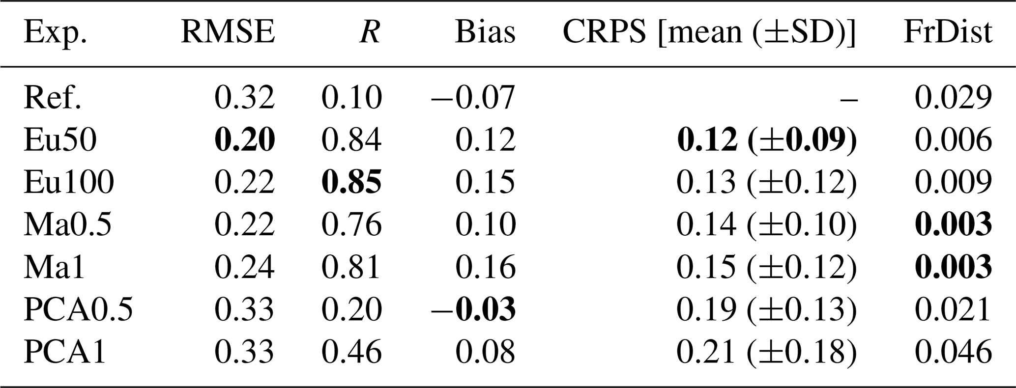
Unfortunately, despite the convenience of using a PCA preprocessing step, the experiments using PCA exhibited only a slight improvement in some metrics while degrading other indicators. In particular, they exhibited a slight improvement in the correlation values (R=0.20 and 0.46 for PCA0.5 and PCA1 respectively), while all other metrics were similar to the reference (e.g. bias), with a FrDist being equivalent or significantly degraded relative to the reference for the PCA0.5 (FrDist = 0.021) and PCA1 (FrDist = 0.046), respectively. This suggests not only that absolute error metrics were not improved, but even that spatial patterns were not adequately simulated with the PCA approach.

Among the Eu experiments, Eu50 exhibited slightly better or similar error metrics than the Eu100. However, the differences were minimal, suggesting there is flexibility in choosing the GC hyperparameters, in this case at least, in terms of validation metrics. A similar conclusion can be drawn from the validation metrics of the Ma experiments, where there was not a clearly superior simulation. Similarly, Eu and Ma yielded comparable performance according to these error metrics. However, the FrDist metric was consistently lower in the Ma experiments compared with the Eu experiments, suggesting a better representation of the spatial patterns, while the remaining error metrics were slightly better or similar for the Eu experiments. This superior performance in representing the spatial patterns was evident in the snow depth semivariograms of the experiments (Fig. 2), where Ma experiments exhibited a semivariance much closer to the observations, even reproducing accurately the nugget effect exhibited by the observations, suggesting a better representation of the small scale patterns. In any case, the variograms of the Eu and Ma experiments exhibit a closer shape to the one obtained from the observations, compared with the one obtained in the reference run, which is nearly flat.

Figure 2 Snow depth spatial semivariance derived from the lidar-derived observations, the reference run and different experiments.

When examining the distributed posterior mean simulations, these considerations about the spatial patterns become evident (Fig. 3). First, there was a very limited spatial variability in the deterministic reference run, as reflected quantitatively by the Frechet distance and qualitatively by the variograms. Among the Eu50 and Ma0.5 posterior maps, there is a clear difference in its snow depth spatial patterns. While the large scale patterns were similar in both simulations, and close to the observations, the small scale patterns were different. In Eu50 small scale patterns of the posterior mean were clearly affected by the shape of the GC function, since the blurrier horizontal patterns are reminiscent of the Gaussian-like shape of this function. On the other hand, Ma0.5 small scale patterns, which do not depend solely on geographic distance, are considerably more intricate, which also explains the lower FrDist error metric.

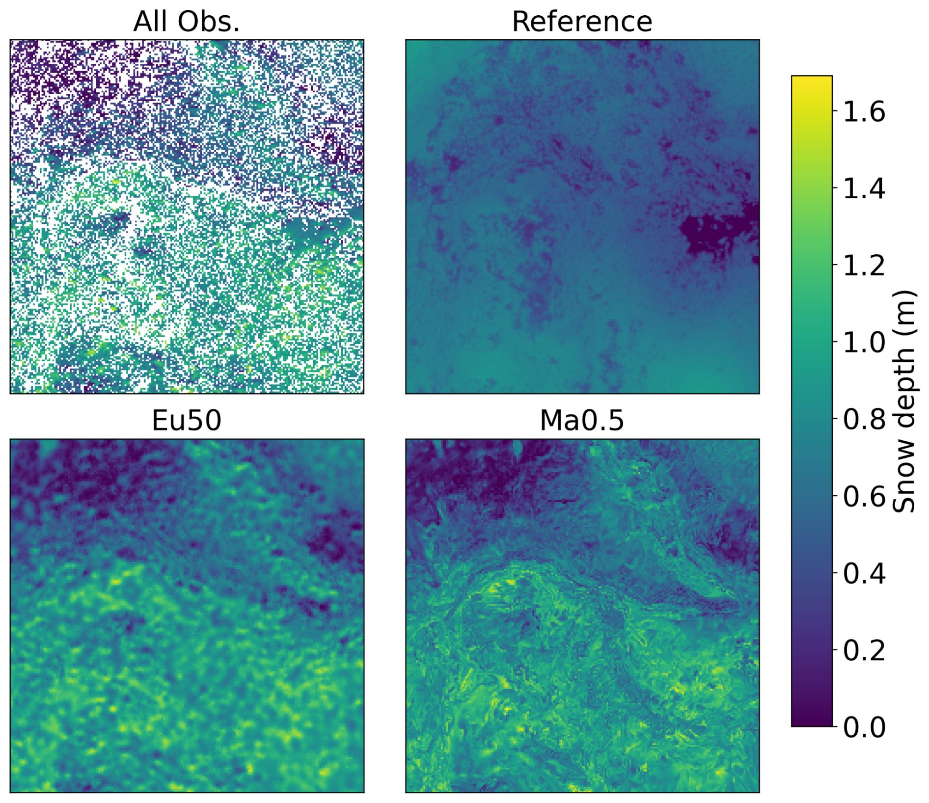
Figure 3 Distributed snow depth observations, reference simulation and posterior mean simulations of the Eu50 and Ma0.5 experiments.

While both in Ma0.5 and Eu50 point scale comparison with observations show a similar overall R metric and distribution, it is worth noting the differences shown in Fig.4. In Ma0.5, the cells with local observations (i.e. the cells in the forest gaps, which include assimilated information) exhibit slightly larger residuals (R=0.99 and R=0.97 for Eu50 and Ma0.5 respectively). These differences suggest that the influence of the GC hyperparameter makes both schemes not fully comparable. This is a consequence of the varying number of observations used to update the parameters of each cell that differ for each experiment, depending on how much space falls within the correlation length scale of the GC function in each case.

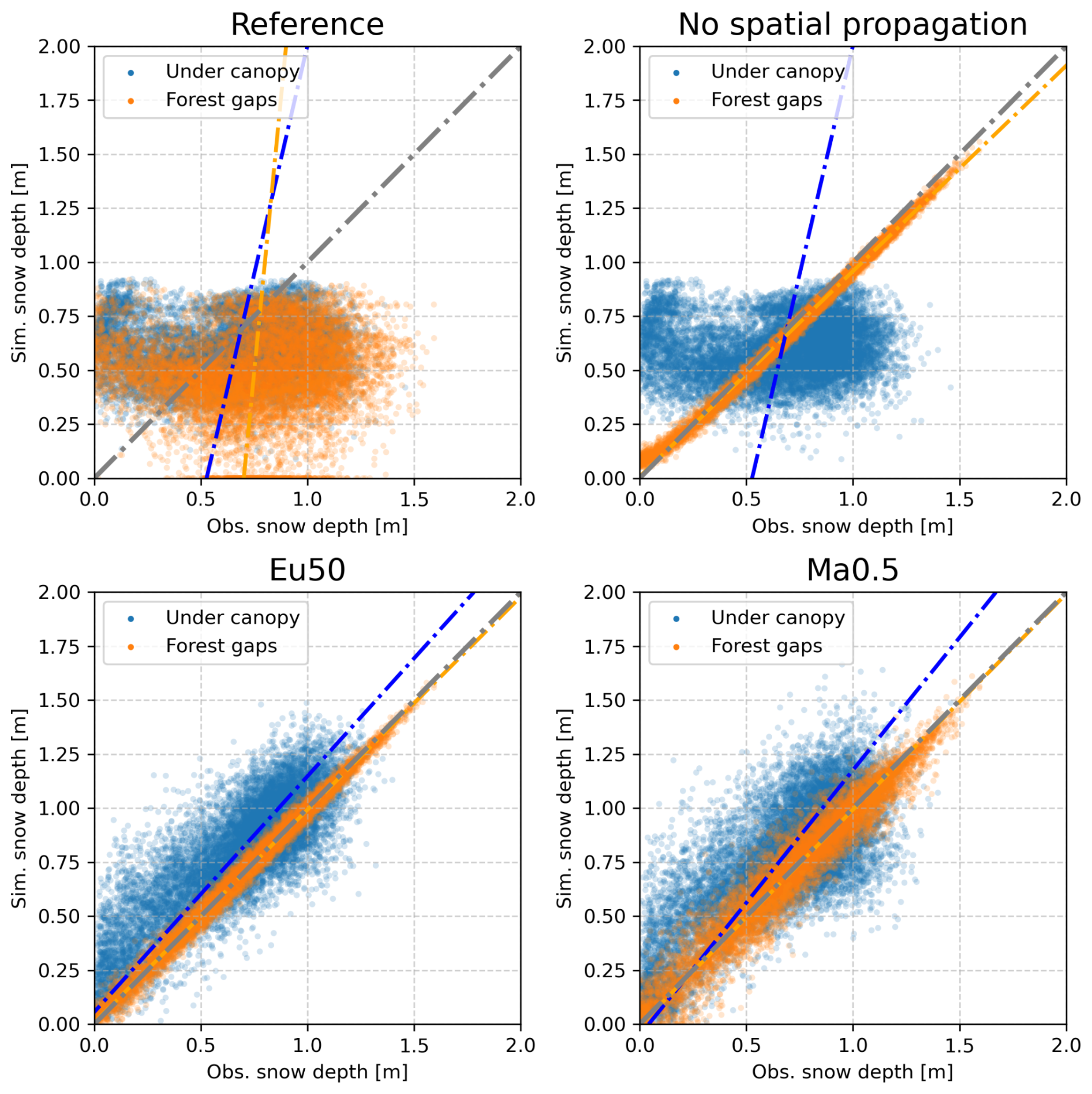
Figure 4 Scatterplot based comparison of the under canopy (withheld) and forest gaps (assimilated) observations, with the reference simulation, and the posterior mean of a data assimilation experiment without and with the spatial propagation of the information enabled (experiments Eu50 and Ma0.5)

However, these error metrics should be taken with care. Most of them (except CRPS) used the posterior mean as an optimal point estimate of the updated simulation. This assumption was adopted for simplicity but may compromise the interpretation of the results. Posterior simulations are not deterministic simulations and come with an uncertainty estimate inherent in the posterior ensemble. To investigate this issue, we extracted a longitudinal profile along the easting dimension, including both the deterministic reference simulation and the posterior mean, but for the latter we now included the associated uncertainty represented by ±1 posterior standard deviation (which accounts for approximately 68 % of the posterior probability, Fig. 5). In addition, we included a representation of the observations obtained both beneath the canopy and in forest gaps. The profile highlights the differences of using the GC function in the Euclidean or topographic space, with Eu exhibiting a much smoother surface compared with the sharper Ma profile. Both profiles exhibited a similar performance if we account for the uncertainty. In terms of the posterior mean, Ma0.5 was able to accurately capture snow depth in large areas beneath the canopy (e.g. Fig. 5 from 1000 to 1250), while maintaining most of the observations in at least the range of its standard deviation. Both Eu50 and Ma0.5 improved the reference run, which exhibited an evident underestimation and lack of heterogeneity along this profile, with only a few observations approaching the simulated reference values.

Figure 5 Snow depth profile showing the match between the reference run (black line), the Eu50 and Ma0.5 experiments and the observations for the horizontal profile delineated by the red line shown in Fig. 1. The dark blue line is the posterior mean and the shaded area the posterior standard deviation.

3.2 Posterior parameters

Although the aim of the present work is to explore how to propagate the information spatially, it is tempting to analyze the posterior distribution of the parameters (Fig. 6). On average for all cells, using the experiment Ma0.5 as a reference, the multiplicative precipitation parameter was 1.06 (±0.30) and the additive temperature parameters was −0.04 (±0.73). Figure 6 should be interpreted with caution. It is designed to provide a rough estimate of the posterior parameter values. However, drawing conclusions beyond that is risky, since there is likely to be equifinality in the parameter posteriors of the simulations, something that is merely suggested by the obvious correlation between the posterior mean parameters.

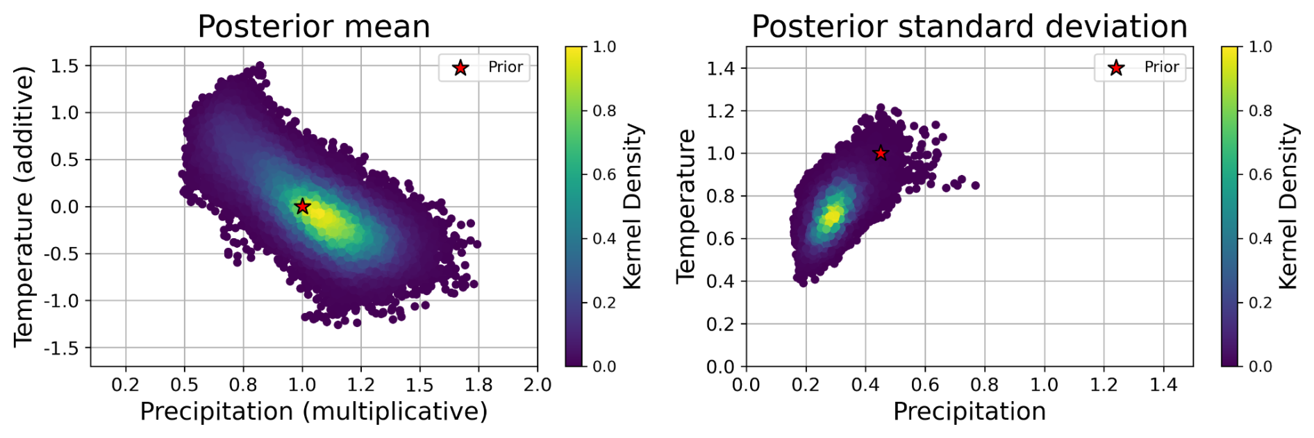
Figure 6 Posterior distributions of perturbation parameters in the model space for the Ma0.5 experiment, each point represents a grid cell.

4 Discussion

The results shown here demonstrate the potential of ensemble-based DA experiments to improve hyper resolution snowpack simulations in forested terrain, by updating the canopy covered cells from information retrieved in clearings. Recall that the DA schemes proposed herein are theoretically independent of the underlying numerical model, meteorological forcing or site. As such, in practice any other snow or land surface model forced by meteorological data generated by any downscaling tool at any geographical location may benefit from the proposed techniques. The aim of this work is not to perform the best possible simulation, but to explore whether it is possible to improve snowpack simulations in forested areas by means of DA. Future initiatives may choose to explore the added value of including additional forcing corrections or internal model parameters in the parameter vector since there is, in theory, not any particular limitation on this provided that a large enough ensemble is computationally feasible.

All experiments were performed using the Centre National D'Etudes Spatiales (CNES) supercomputing infrastructure. For reference, the Ma0.5 experiment took one day and eight hours to complete, using 6 nodes with 10 CPUs each to solve the 40401 cells (201 cells in each geographical direction) that compose the domain using the aforementioned DA scheme. This estimate of computational cost, which could be considered very affordable, especially given the iterative nature of the assimilation algorithm and the relatively low number of processors involved, should be treated with some caution. The computational time varied significantly between experiments, as in practice the I/O increases with the GC hyperparameter, which effectively defines a search radius. In addition, MuSA benefits from distributed systems that share I/O bottlenecks among their nodes, so the computational scheme can also be very relevant. On the other hand, other DA experiments with a lower density of observations will see their computational cost dramatically reduced, independent of the GC hyperparameter.

Most of the DA configurations managed to improve the posterior simulations compared with the deterministic reference simulation, with different configurations showing similar error metrics. However, the PCA based experiments, despite their desirability given the orthogonal properties of the synthetic coordinate system, did not perform as expected. We hypothesize that the limitations found may come from the fact that the new set of coordinates do not explicitly preserve the Cartesian northing and easting information by mixing them with other dimensions, relaxing the relations between nearby cells in the Euclidean space (Davis and Curriero, 2019). However, the same could be said when using the Mahalanobis distance, but the performance of the Ma experiments was clearly superior compared to the PCA ones. A potential reason may be the fact that, to ease the positive-definiteness of the PCA-based covariance matrix by sorting the cells in a lower dimensional space, we used the Minka algorithm to reduce the dimensionality of the synthetic coordinate system. This dimension reduction comes in practice with a loss of information. However, this is very unlikely, since in practice it resulted in only one dimension being removed, which represented a very low percentage of the total variance of the system. This requires further research to fully understand how the information can be effectively propagated in different spaces. A potential future approach may be the use of multidimensional scaling techniques, instead of PCA, that have shown previous success in geostatistics (Murphy et al., 2015). The challenges previously encountered in generating non-positive definite covariance matrices have been substantially mitigated. Previous research has proposed to enforce positive definiteness in covariance matrices by using (potentially iterative) methods based on eigendecomposition, to make any negative eigenvalues of the covariance matrix become nonnegative (e.g. Davis and Curriero, 2019 and references herein), which imposed a considerable computational burden, particularly for large matrices. However, regularizing the covariance matrix with the introduction of the jitter technique (where small values are iteratively added to the diagonal) has proven to be both highly effective and computationally efficient. Whether the results of prior sampling differ significantly between these two approaches to regularize the covariance matrix remains an open question for future investigation.

In these experiments we update meteorological correction parameters only, and not snowpack states, allowing the numerical model to resolve the snow-canopy interactions. This prevents the posterior simulations to be degraded by the fact that in reality the snowpack beneath the canopy behaves differently than in open terrain (Pflug et al., 2024; Varhola et al., 2010), by updating only parts of the simulation that we assume to be similar independently of the canopy cover (such as the precipitation or temperature), and letting the model to resolve the parts that can't be constrained (such as snow states), due to the lack of information.

Since the main objective of this experiment was to explore how the information can be propagated effectively from clearings towards the canopy covered cells, we split the observation dataset in two, keeping the cells beneath the canopy for validation. This has not allowed us to include vegetation parameters in the distance mapping of the Ma experiments, as the cells inside and outside the forest would have been too far away in Mahalanobis space, and therefore due to the localization, the information would not have been transmitted from the clearings towards the sub-canopy. Some vegetation model parameters could have been included in the inference, but because the information is located in the forest gaps, they could not have been constrained. However, given the success of the experiments, future research would benefit from assimilating data also in canopy-covered cells, if a proper error model is developed. State of the art remote sensing techniques are able to retrieve at least a partial information of the snowpack in forested terrain (Mazzotti et al., 2019), or even snow cover information from satellites (Xiao et al., 2022). This may be used not just to further improve the posterior simulations but as a tool to infer internal model parameters spotting weakness in canopy/snow models or their parameters.

It should be noted that these spatio-temporal techniques are compatible with joint DA initiatives, where more than one type of observation is assimilated into the same simulation, potentially only spatially spreading some of them (Mazzolini et al., 2025). This may include the ingestion of under canopy in situ observations jointly with remotely sensed retrievals of any kind. It is worth noting that, due to the assimilation of only a single incomplete snow distribution map, the posterior simulations exhibit equifinality (Beven and Freer, 2001), which prevents us from exploring in detail which of the parameters (precipitation or temperature correction) is more dominant over the other since they are correlated (Fig. 6). Adding other data sources and using more varied information could help address this issue in future studies. In any case, the mean posterior values obtained were close to unity for precipitation (in the physical space) and close to zero for temperature, suggesting that it is not the total amount of precipitation that is biased, but rather the small-scale redistribution of the meteorological forcing.

Among the experiments that improved the simulations compared with the deterministic reference run, there was not a clearly superior experiment depending on the GC correlation length scale hyperparameter. Similar conclusions could be drawn from the findings in Cho et al. (2023), who tested different correlation length scales for their Gaussian decay-based localization function, showing that the differences were always lower than the improvement compared with their reference simulation. This suggests some flexibility in the choice of this hyperparameter, which may be complex especially when using non-Euclidean distances, and often limited by the availability of considerable computing resources.

When comparing the Eu and Ma experiments, it was also difficult to spot differences if considering only quantitative error metrics. However, the spatial patterns at smaller scales seem more realistic when using the Ma configuration, as also found in Alonso-González et al. (2023a). This is based on the fact that the snow spatial patterns are correlated with the characteristics of the terrain, since it controls its distribution by modulating accumulation and melt processes in both open and forested terrain (Geissler et al., 2025; Revuelto et al., 2014). The proposed domain is relatively small exhibiting a limited topographical complexity. Other experiments over larger areas of increasing topographical complexity may benefit from the increasing topographical variability. A potential limitation of this method will be found in non-complex terrain, as is typical in high latitude areas, where the topographical control of the snowpack dynamics may be less clear, although still very relevant (Bennett et al., 2022). In any case, snowpack in these areas exhibits less spatial variability, so we hypothesize that the use of Euclidean distance to map cell similarity is likely to be sufficient in these environments and/or at coarser resolutions.

Alternatively, it is possible to use snow climatologies or observations to perform a more direct cell similarity mapping based on the persistence of the spatial patterns of the snow (Alonso-González et al., 2023a; Mazzolini et al., 2025). Despite developing snow cover climatologies in forest environments is significantly more challenging than in open terrain due to the aforementioned limitations of satellites to retrieve information beneath the canopy, it is possible to generate maps of the snow distribution in forested terrain by combining different techniques such as ground observations, lidar and field campaigns (Geissler et al., 2023). The generation of such products requires a significant effort in logistics that prevent its operational exploitation as a real time monitoring tool. In addition, such field methods will not be able to retrieve information at other times that the observation time itself. A promising application of the assimilation scheme presented here is to exploit such products to map the similarity between cells in forested terrain, allowing the significant effort needed for these initiatives to be exploited to generate gap-free re-analyses or near real time updated simulations.

In this work, we have explored the effect of using the GC function to create a prior covariance matrix in different spaces. However, what remains to be investigated is the potential benefit of using different covariance (or kernel) functions. It is possible that other functions may offer a more accurate representation of snowpack correlograms across various spatial scales and resolutions, especially in topographical Mahalanobis spaces. One obvious source of inspiration is to take advantage of the extensive literature on kernels developed by the Gaussian process community (Rasmussen and Williams, 2005). In particular, kernels with compact support – those that become zero beyond a certain boundary – (Barber, 2020) could be of special interest since they will behave similarly to the GC function, helping in limiting the computational cost and preventing spurious correlations among the ensembles. Given the increasing availability of snow depth information over large domains (Magnusson et al., 2025; Painter et al., 2016), it will be beneficial for the snow DA community to explore which kernel functions better approximate the empirical snowpack spatial variability in different spaces and resolutions. Given that snowpack exhibits persistent spatial patterns in both forest and open terrain (Geissler et al., 2025; Helfricht et al., 2014), there is potential to find a single flexible kernel configuration, ideally depending on a very limited number of parameters, to be widely used in both spatiotemporal DA and observation interpolation initiatives.

5 Conclusions

In this work, we have explored the potential of the observations obtained in forest clearings to be used to update spatially complete snow simulations in forest environments by means of spatio-temporal ensemble-based data assimilation. Six different experiments were conducted in the Sagehen Creek (California, USA) using different data assimilation configurations, demonstrating the potential obvious benefits of spatiotemporal DA in forest environments. While most of the experiments greatly improved the reference snow simulations, those relying on a set of synthetic dimensions generated by a PCA were clearly inferior. Future research may benefit from exploring other dimension reduction techniques such as multidimensional scaling. Among the remaining successful experiments, there was not a clearly superior configuration, in that the differences among them were significantly lower than the improvement compared with the reference run. This suggests some flexibility on the selection of the critical hyperparameters of the DA. However, we found that in terms of both qualitative and quantitative error metrics, those experiments built on a cell similarity mapping based on the Euclidean distance were slightly more accurate in terms of absolute validation metrics, but with a more realistic representation of the spatial variance when using the Mahalanobis distance in a topographical space. This suggests that this latter technique is better suited for preserving spatial relationships in complex terrain. The differences found in the implementation of the prior covariance function in the Mahalanobis and Euclidean spaces, suggests the importance of future research investing effort in exploring of specific covariance function that better capture the snowpack spatial patterns