The Greenland Ice Sheet Large Ensemble (GrISLENS): simulating the future of Greenland under climate variability

The Greenland ice sheet has lost ice at an increasing pace over recent decades, driven by a combination of human-caused climate change and internal variability in the climate system. In projections of future ice sheet evolution, internal variability in climate results in uncertainty that cannot be reduced through model improvements due to the intrinsically chaotic nature of the climate system. This study describes the Greenland Ice Sheet Large Ensemble (GrISLENS), the first large-ensemble study of ice sheet evolution under climate variability, which resolves individual outlet glaciers and climate variability calibrated to observations. GrISLENS combines multiple advanced modeling methods, including a stochastic ice sheet model, a coupled atmosphere–ocean model, dynamical surface mass balance downscaling, and statistical techniques for constraining stochastic parameterizations of climate forcing. We quantify the role of internal climate variability in 185-year projections of the Greenland ice sheet under both a high-emission scenario and pre-2000 climate conditions. We find that spread between ensemble members due to internal climate variability represents a substantial fraction of the mean ice sheet change in the first 20–30 years of simulations, which may be important for coastal planning efforts on decadal timescales. This spread between ensemble members decreases to a small fraction of the total ice sheet change past 2050. At the ice sheet scale, uncertainty in ice loss is dominated by the response to surface mass balance variability, while the response to ocean variability is relatively small, though its influence is more important within individual catchments. The GrISLENS ensemble spread is relatively small compared to that of previous studies estimating uncertainty from climate variability in coarse models, which indicates that resolving small-scale features in climate forcing and ice sheet dynamics substantially affects the quantification of internal variability in ice sheet mass change. On longer timescales, human emissions of greenhouse gases and structural and parametric uncertainties in climate and ice sheet models are larger contributors to projection uncertainties. Through our analysis, we identify the need for more robust initialization methods and extension of these large-ensemble methods to the Antarctic ice sheet.

1 Introduction

Mass loss from the Greenland ice sheet (GrIS) has contributed ∼16 % of total global sea level rise since 1992 (IPCC, 2021), driven by increasing surface melt (Fettweis et al., 2016) and accelerated ice discharge into the ocean (King et al., 2020). GrIS mass loss is also rapidly accelerating: the mass loss from 2012 to 2020 was more than 5 times the mass loss from 1992 to 2000 (Otosaka et al., 2023). Over the 21st century, the projected contribution of the GrIS to sea level rise is sensitive to both the greenhouse gas emission scenario and the internal variability in the climate system (Tsai et al., 2017). While quantifying the ice sheet's sensitivity to greenhouse gas emissions has been the focus of substantial community efforts (Nowicki et al., 2013; Goelzer et al., 2020), less attention has been paid to quantifying the range of possible future ice sheet evolution due to internal variability in the climate system alone.

Projections of future GrIS mass balance are generally determined from ice sheet model simulations, with prescribed climatic forcing (e.g., Goelzer et al., 2020). A number of factors contribute to uncertainties in ice sheet model projections (Aschwanden et al., 2021). First, structural model uncertainty stems from our incomplete understanding of processes regulating ice sheet dynamics, such as iceberg calving (Amaral et al., 2020), subglacial hydrology (Kazmierczak et al., 2022), basal sliding (Choi et al., 2022), and ice mélange (Joughin et al., 2020). Second, some processes are not fully resolved by the typical spatial resolution and time steps in ice sheet models. This can be due to insufficient knowledge of fine-scale mechanisms or computational limitations. Such processes are parameterized using physical mechanisms and observational constraints, but the high number of unknown parameters in such calibration procedures implies that numerical parameter values remain uncertain (Wernecke et al., 2020; Berends et al., 2023). Third, uncertainty in initial conditions impacts simulations over long periods and therefore projections (Adalgeirsdottir et al., 2014; Yang et al., 2022). Imperfect knowledge of the current and past states of the GrIS has a long-lasting influence on ice sheet evolution and observational errors in ice sheet geometry and other observational fields (Seroussi et al., 2011). To evaluate the total uncertainty arising from these sources, ice sheet model intercomparisons are performed, in which each participating model may include different physical processes, initialization methods, parameter schemes, and numerical schemes (Goelzer et al., 2020). The results of such intercomparisons (the most recent being ISMIP6, Goelzer et al., 2020) have been used as the primary source for sea level projections by the Intergovernmental Panel on Climate Change (IPCC, 2021) and related efforts (Edwards et al., 2021).

Projections of ice sheet mass balance are also influenced by the inherent uncertainty associated with future climate variability (Mikkelsen et al., 2018; Robel et al., 2019). For any given scenario of anthropogenic forcing, there remains an “irreducible” (also called “aleatoric”) uncertainty associated with the ice sheet response to internal climate variability due to the fundamental unpredictability of the climate system (Lorenz, 1969). It is common practice in the climate modeling community to quantify internal variability through large ensembles, sampling different initial conditions and multiple realizations of each climate model (Mankin et al., 2020; Deser et al., 2020). However, current ice sheet model intercomparisons are not designed to quantify this aleatoric uncertainty, as they typically force ice sheet models with a single realization from each combination of climate models and emissions scenario selected (e.g., Goelzer et al., 2020; Li et al., 2023). Yet, idealized studies have demonstrated the sensitivity of glacier evolution to processes that have comparable timescales inherent to internal climate variability (Roe and Baker, 2016; Mikkelsen et al., 2018; Robel et al., 2018; Christian et al., 2020; Verjans et al., 2022). For example, processes that are poorly represented in climate models, such as atmospheric blocking (Hanna et al., 2018), might have an important effect on GrIS projections (Beckmann and Winkelmann, 2023). Despite this known strong sensitivity of the GrIS to climate forcing, sensitivity to internal climate variability and associated irreducible uncertainties remain poorly quantified (Aschwanden et al., 2021).

To understand the importance of internal climate variability for ice sheet mass balance over the next 200 years, large-ensemble experiments are a viable approach. In recent years, global climate model (GCM) large ensembles have been produced and made available as community data sets (e.g., Kay et al., 2015; Rodgers et al., 2021). This has enabled the investigation of many questions, such as possible future changes in modes of climate variability (Zheng et al., 2018), sensitivity of the overall climate variability spectrum to forcing (Rodgers et al., 2021), attribution of extreme-weather events to anthropogenic forcing (Diffenbaugh et al., 2017), and evaluation of the range of possible socioeconomic impacts of climate change (Schwarzwald and Lenssen, 2022). Internal climate variability has also been extensively explored through observational studies (Mitchell, 1976; McKinnon et al., 2017). This inherent feature of the climate system therefore deserves attention, including its impacts on the evolution of the GrIS.

Tsai et al. (2017) attempted the only prior study on the role of internal climate variability in the evolution of the GrIS. Their approach used 40 and 50 members of two different coarse GCM large ensembles as direct climate forcing for Greenland ice sheet model simulations over the 21st century. They found that, under a high-emission scenario, the spread in sea level rise contribution by 2100 between ensemble members is ∼17 % of their ensemble mean simulated ice sheet mass loss. However, this method faces two limitations. First, the coarse resolution of GCM outputs (∼100 km grid scale, monthly time steps) implies limited representation of processes with strong spatial gradients. Second, GCM outputs do not correspond directly to inputs needed for ice sheet models, and thus some assumptions have to be made for such conversions, such as simplified empirical relationships between atmospheric temperature and ice sheet surface mass balance. Furthermore, Tsai et al. (2017) ran their ice sheet model at a coarse resolution over the GrIS (20 km), therefore potentially not resolving individual outlet glaciers, almost all of which are less than 20 km wide in Greenland. The use of such a coarse resolution has been shown to induce substantial quantitative impacts on ice sheet model results (Greve and Herzfeld, 2013). Still, the results of Tsai et al. (2017) have demonstrated that uncertainty associated with internal climate variability may amount to a non-negligible fraction of future GrIS change and may persist on decadal to centennial timescales.

In this study, we describe the Greenland Ice Sheet Large Ensemble (GrISLENS), a modeling experiment estimating the GrIS sensitivity to internal climate variability down to sub-kilometer scales. We apply a novel stochastic modeling approach to address this question. Specifically, we calibrate spatiotemporal stochastic models to downscale GCM outputs and subsequently use them to force ice sheet model simulations spanning 2018 to 2203. Our results quantify model spread in GrIS mass change, ice thickness change, and glacier retreat, all associated with internal climate variability. We compare this spread with ensemble mean change under different mean forcings and with differences in projected ice sheet mass between different ice sheet and climate models from prior intercomparison studies. Finally, we make our model output openly available to enable future investigations into the role of internal climate variability in driving ice sheet change, similar to the growing use of large-ensemble climate model outputs in climate sciences.

2 Methods

The ensemble of simulations presented in this study is the culmination of prior work to develop methods which can stochastically generate realistic climate forcing for ice sheet models down to sub-kilometer spatial scales. At the base of these methods is output from a climate model spanning both the historical period over which the ice sheet model is initialized and a period of several centuries into the future over which the evolution of the GrIS is expected to unfold. Atmospheric forcing is then converted and downscaled to surface mass balance (SMB) using a high-resolution energy-balance model (Krebs-Kanzow et al., 2020) and used to calibrate a stochastic SMB parameterization for every glacier catchment in Greenland using the method described by Ultee et al. (2024). Ocean forcing is calibrated to available observations of ocean properties around Greenland, downscaled to fjords, and then used to calibrate stochastic parameterizations of ocean thermal forcing for every marine-terminating glacier catchment in Greenland using the method described by Verjans et al. (2023). The stochastic parameters of these methods are then input directly into the Stochastic Ice-Sheet and Sea-Level System Model (StISSM; Verjans et al., 2022), which internally generates realistic and correlated climate variability to force the ice sheet model equations. While the details of these methods can be found in the studies cited above, additional methodological developments needed for this study are described below. All model output discussed in this study and the code used to generate figures are openly archived in a persistent repository at the Arctic Data Center (Robel et al., 2025).

2.1 Ice sheet model forcing

For our simulations, stochastic realizations of the three climatic variables are generated (as described in detail below) within the ice sheet model, the Stochastic Ice-Sheet and Sea-Level System Model (StISSM; Verjans et al., 2022). StISSM generates noise, computes the corresponding time series (Eq. A2), and performs the SMB lapse rate corrections within the evolving ice sheet simulation. Within each catchment, local spatial variations in SMB (Λ(z)) and feedbacks with ice sheet elevation are represented through a simple piecewise function of elevation:

$$\begin{array}{}\text{(1)}& \mathrm{\Lambda }\left(z\right)=\left\{\begin{array}{ll}{c}_{\mathrm{0}}+c_{\mathrm{1}}z& \mathrm{0}<z\le z_{\mathrm{1}}\\ c_{\mathrm{0}}+c_{\mathrm{1}}{z}_{\mathrm{1}}+c_{\mathrm{2}}z& z_{\mathrm{1}}<z\le z_{\mathrm{2}}\\ c_{\mathrm{0}}+c_{\mathrm{1}}{z}_{\mathrm{1}}+c_{\mathrm{2}}{z}_{\mathrm{2}}+c_{\mathrm{3}}z& z_{\mathrm{2}}<z\left(\mathbf{p}\right)\le z_{\mathrm{3}},\end{array}\right.\end{array}$$

where c₀ is the minimum SMB, and the segment slopes $(c_{\mathrm{1}},c_{\mathrm{2}},c_{\mathrm{3}})$ and breakpoints (z₁,z₂) are free parameters that must be calibrated. Stochastic catchment-wide anomalies in SMB are generated using a method described in brief below and in detail in Ultee et al. (2024). Doing these computations within the ice sheet model is preferable to capture feedbacks with ice sheet geometry (on SMB in particular) and correlations between climate forcing variables and to avoid uncertain conversions from inputs to ice sheet model quantities. Runoff and thermal forcing (TF) are used as forcings for a parameterization of frontal melt rate (${\dot{m}}_{\mathrm{fr}}$) at a grounded marine-terminating glacier, as described by Rignot et al. (2016):

$$\begin{array}{}\text{(2)}& {\dot{m}}_{\mathrm{fr}}=(A{h}_{\mathrm{w}}{q}_{\mathrm{sg}}^{\mathit{\alpha }}+B){\text{TF}}^{\mathit{\beta }},\end{array}$$

where q_sg is the subglacial water flux [m d⁻¹], and h_w is the water depth [m]. The calibration parameter values are $A=\mathrm{3}\times {\mathrm{10}}^{-\mathrm{4}}$ m^−α d^α−1 K^−β, B=0.15 m d⁻¹ K^−β, α=0.39, and β=1.18 (Rignot et al., 2016). We substitute the catchment-integrated runoff generated by StISSM for q_sg, thus assuming that all the runoff over a given time step is discharged immediately at the marine front in catchments in contact with the ocean.

For floating ice, we follow a simplification of the “three-equation” melt parameterization (Holland and Jenkins, 1999; Beckmann and Goosse, 2003):

$$\begin{array}{}\text{(3)}& {\dot{m}}_{\mathrm{fl}}={\mathit{\rho }}_{\mathrm{w}}{c}_{p\mathrm{M}}{\mathit{\gamma }}_{\mathrm{T}}{F}_{\mathrm{m}}\text{TF},\end{array}$$

where ρ_w is the ocean water density (1023 kg m⁻³), c_pM is the ocean mixed-layer specific heat capacity (3974 J kg⁻¹ K⁻¹), γ_T is the thermal exchange velocity (10⁻⁴ m s⁻¹), and F_m is an empirical melt factor set to 0.203 following Favier et al. (2019).

2.2 Climatic forcing

2.2.1 Reference climate model simulation

Atmospheric and ocean forcing for our Greenland simulations is based on a 1850–2203 simulation of the Alfred Wegener Institute Earth system model (AWI-ESM; Ackermann et al., 2020). The ocean model implemented in AWI-ESM is FESOM1.4 (Wang et al., 2014). It employs an unstructured grid with a resolution of ∼20 km around Greenland. The atmosphere is represented with the ECHAM6 model (Stevens et al., 2013) using a horizontal resolution of 1.85° (50–100 km across Greenland). After the historical period 1850–2005, the simulation that we use follows the high-emission scenario RCP8.5 (Riahi et al., 2007) until 2100 and keeps the atmospheric CO₂-equivalent forcing fixed at the 2100 level for the 2101–2203 period. We note that in recent GCM intercomparisons, AWI-ESM shows behavior close to the multi-model average in terms of key climatic features, such as equilibrium climate sensitivity and transient climate response (Semmler et al., 2020).

2.2.2 Atmospheric forcing

AWI-ESM atmospheric fields over Greenland are downscaled at 5 km horizontal resolution using the diurnal Energy Balance Model (dEBM; Krebs-Kanzow et al., 2020). In a recent intercomparison of SMB from different regional climate models (Fettweis et al., 2020), dEBM GrIS-averaged SMB was shown to be less than 20 % of the ensemble standard deviation from the ensemble mean SMB and to exhibit temporal dynamics within the uncertainty range of gravimetry observations. We use the SMB and runoff output fields from dEBM, and we process these variables at the catchment level. Specifically, we use the 253 catchment delimitations of Mouginot et al. (2017) over the contiguous GrIS. We take the average SMB and the total runoff over each catchment and aggregate the monthly values at an annual resolution. As such, each catchment has a single 1850–2203 annual time series for both SMB and runoff, which can serve to calibrate stochastic time series in the models, as detailed in Sect. 2.2 (see also Ultee et al., 2024). In this study, we regard SMB as an annual variable, as sub-annual variability in SMB is unlikely to play a strong role in ice sheet dynamics over decadal to centennial timescales (Robel et al., 2019; Christian et al., 2020). However, we do account for monthly variability in runoff by computing the average fraction of the annual runoff occurring in each month for each individual catchment, since monthly runoff affects melt at the ocean interface (see Sect. 2.2.3). Within-catchment spatial variability in SMB is captured through the estimation of the slope of SMB–elevation profiles, as described in Ultee et al. (2024). Further details and examples for this specific study can be found in Appendix B.

2.2.3 Ocean forcing

Ocean forcing for the ice sheet model is derived from variations in ocean temperature and salinity simulated by AWI-ESM. In our ice sheet modeling framework, the ocean melt rate parameterization uses thermal forcing (TF), the water temperature above freezing point. TF is integrated through depth to calculate parameterized melt rates at glacier fronts. As waters around Greenland are stratified, generally with cold and fresh Arctic water above warmer and saltier Atlantic waters (Straneo et al., 2012), the depth range over which TF is integrated strongly influences the melt rates calculated. We find the effective depth of each Greenland marine-terminating glacier, which is defined as the deepest bathymetry connected to the open ocean without a barrier (e.g., Morlighem et al., 2019; Slater et al., 2020). We use the BedMachine v4 product for the bathymetry around Greenland (Morlighem et al., 2017). For each marine-terminating glacier, we integrate TF from the surface until its effective depth (which does not vary with ice sheet evolution), and each glacier is thus assigned a specific field of depth-integrated TF time series. For a detailed discussion of this choice of method for calculating TF, see Appendix C. Throughout this study, we use the notation TF to refer to this depth-integrated value. We further adjust the AWI-ESM TF following a two-step procedure, as summarized below and detailed at length in Verjans et al. (2023).

First, we bias correct the AWI-ESM TF based on the EN4 ocean monthly objective analyses (Good et al., 2013). EN4 is an interpolated product of ship-based oceanic observations, which is constrained more closely to observations compared to dynamical reanalysis products. Though this interpolation ensures better agreement with in situ data, EN4 is more prone to errors in the case of observational uncertainties and if some periods and/or regions have sparse observational coverage. For each AWI-ESM grid point, we perform the bias correction with the nearest EN4 grid point using the 1950–2006 TF from AWI-ESM and EN4, which corresponds to the pre-RCP8.5 forcing in AWI-ESM. The period before 1950 is not used for the bias correction because EN4 is poorly constrained by observations (Verjans et al., 2023). The bias correction follows a quantile-delta-mapping procedure (Cannon et al., 2015; Verjans et al., 2023). This procedure calibrates both the mean and the amplitude of variability in AWI-ESM to EN4 while preserving the relative changes in time of TF as modeled by AWI-ESM.

Second, we downscale the bias-corrected TF from the AWI-ESM grid to fjord mouths. The extrapolation is based on statistical relations found between shelf waters and fjord mouth conditions in the output of a high-resolution ocean model reanalysis, ECCO2-Arctic (Nguyen et al., 2012). These statistical relations are derived for the long-term mean TF and for the seasonal and non-seasonal variability. The fjord mouth locations are selected as the closest ECCO2-Arctic grid point to each Greenland glacier front from Wood et al. (2021), with bathymetry at least as deep as the effective depth. The data set of glacier fronts includes 226 distinct marine-terminating glaciers.

All our climatic forcing procedures are performed at the catchment scale, but some catchments include no or more than one marine-terminating glacier. As each catchment is assigned a single set of TF statistics, we select a single TF series for catchments with more than one marine-terminating glacier. We select the TF series of the glaciers with the deepest effective depth because these glaciers generally have more impact on the total mass balance of the GrIS. As such, there are 50 glaciers which are assigned a TF time series of a neighboring glacier with a deeper effective depth. For these 50 pairs of time series, the 0.5, 0.75, and 0.95 quantiles of the root mean square deviation are 0.7, 1.5, and 2.1 K, respectively. For the 77 catchments without marine-terminating glaciers, TF does not need to be prescribed.

2.3 Stochastic representation of climatic forcing

2.3.1 Calibration of stochastic climate forcing

Starting from the AWI-ESM outputs, three climatic variables, with time series for each glacier catchment, are post-processed: TF, SMB, and runoff. We separate each annual time series into a deterministic and a stochastic component. The former accounts for the mean forcing and trends, e.g., under the RCP8.5 emissions scenario. The latter accounts for the irreducible uncertainty associated with natural climate variability and is the residual obtained from the original time series by removing the deterministic component. To fit stochastic time series models, the residual variability should be stationary and homoskedastic, i.e., without trends and with constant variance over time (von Storch and Zwiers, 1999). For our three variables, we find that residual variability is stationary if we account for deterministic components that are piecewise linear in time (breakpoints in 2000, 2050, and 2100) and normalize the variance of the residuals (creating a normalized “z-score” series) to account for change in the amplitude of variability over time for each of the three sub-periods. The breakpoints are chosen to capture periods of change in the mean and variability amplitude of climate forcing such that normalized variability is stationary (see below). We chose 2100 as a breakpoint since emissions are held constant after this point in the RCP8.5 climate model simulation described above. We find that just one more breakpoint is needed between 2000 and 2100 to capture the change in the mean and variability amplitude of climate forcing, and for expediency we choose the midpoint of this period. An example of this is illustrated in Fig. 1 for Humboldt Glacier (northeastern Greenland). The original annual time series of our three variables, shown in blue, are well represented by piecewise-linear time series, shown in red. The difference between them is the residual variability, shown in green. The latter is well centered around 0, showing that the secular trends are correctly captured by the piecewise-linear functions with the specified breakpoints. However, the residual variability time series clearly show increasing variance in time. Once normalized, the resulting z-score time series are stationary, trendless, and homoskedastic across time.

To validate our approach for generating standardized residual variability time series, we use the augmented Dickey–Fuller test (Dickey and Fuller, 1981). We have 253 time series for SMB, 247 for runoff because 6 catchments have zero runoff over the entire simulation period, and 176 for TF because 77 catchments have no marine-terminating glaciers, thus resulting in 676 z-score time series in total. The null hypothesis of non-stationarity in the augmented Dickey–Fuller test is rejected with significance for all 676 z-score time series (p values <0.05).

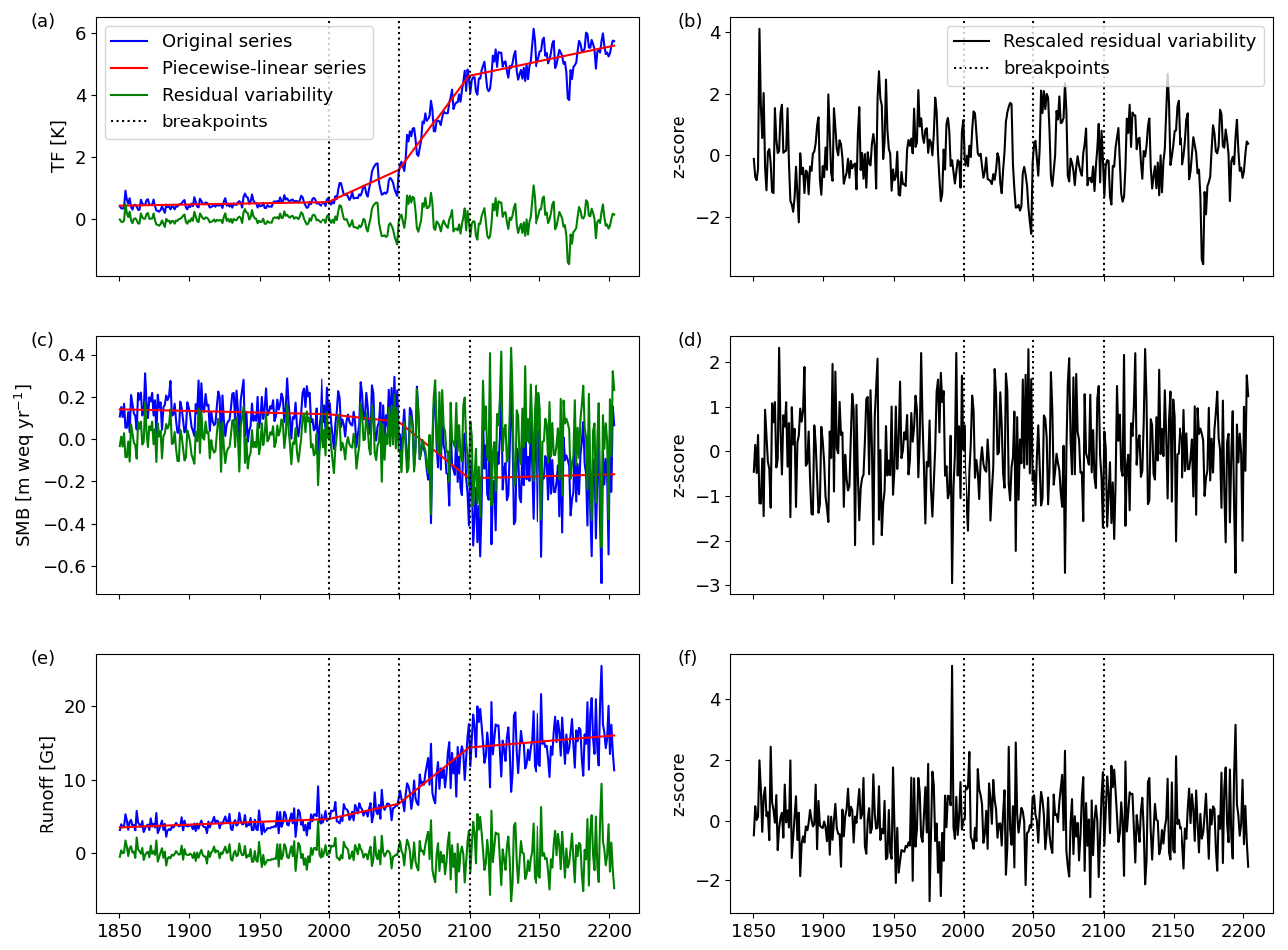
Figure 1 Annual climatic forcing time series at the catchment of Humboldt Glacier (see Fig. 7a for location). Original forcing time series are in blue, fitted piecewise-linear functions are in red, and residual variability is in green. The residual variability is obtained by subtracting the piecewise-linear function from the original series. Breakpoints of the piecewise-linear functions are shown with dotted lines. The residual variability is then standardized to unit variance separately in each sub-period to have unit variance. Standardized residual variability time series are shown in black in the right column. Bias-corrected and extrapolated TF (a) and its rescaled residual variability (b). SMB (c) and its rescaled residual variability (d). Runoff (e) and its rescaled residual variability (f).

We fit stochastic time series models to the annual z-score time series. More specifically, we calibrate an autoregressive moving-average (ARMA) model to each individual time series. ARMA processes are efficient representations of climatic variables, as they can capture an extensive range of timescales while using a small number of parameters (Hasselmann, 1976; von Storch and Zwiers, 1999; Wilks, 2011). Thus, by representing the residual variability component of our climatic variables of interest as an ARMA process, we aim to capture the interannual to decadal timescales of climate variability that force the GrIS climate. Further discussion on the validity of using ARMA models to capture SMB and TF variability can be found in Ultee et al. (2024) and Verjans et al. (2023), respectively.

For each time series, we calibrate all possible combinations of ARMA models with autoregressive (AR) orders and moving-average (MA) orders ranging from 0 to 4. We use the well-established Bayesian information criterion (BIC; Schwarz, 1978) to select ARMA models that best fit the target time series, with a penalty proportional to the number of parameters used. Figure A1 shows the selected ARMA combinations for our three climatic variables and for all the catchments. A large majority of catchments have their SMB and runoff z-score time series best described as an interannual white noise process, which corresponds to an ARMA(0,0) process, i.e., without memory of previous years. Only 39 of the 253 SMB time series and 15 of the 247 runoff z-score series include a lag term (i.e., the p order of ARMA(p,q)). In contrast, only 19 of the TF z-score series are best fitted by annual white noise. Most (70 %) have an ARMA(1,0) as their best-fitting model, and 6 % include a second-order lag term (i.e., ARMA(2,q); Fig. A1). The fact that very few of the best-fitting parameterizations include a moving-average component (q>0) is not surprising and follows considerable prior work (Gilman et al., 1963; Hasselmann, 1976), showing theoretically and empirically that climatic variables are well described as purely stochastic autoregressive processes due to the memory implicit in systems with finite heat capacity.

We account for correlation between all the z-score time series such that time series stochastically generated with ARMA models reproduce the desired level of interdependence between catchments and climatic variables (e.g., Ultee et al., 2024). For this purpose, we calculate the empirical correlation matrix between the residuals of the fitted 676 z-score time series. The residuals are obtained after fitting the optimal ARMA model to a given time series such that the stochastic component ϵ_t (see Eq. A2) is isolated. Isolating residuals allows us to first remove potential spurious correlations between catchments and variables that appear in the raw time series caused by temporal autocorrelation. This autocorrelation is removed from the ARMA residuals, and the remaining correlations found capture cross-spatial and cross-variable dependencies. However, because the number of entries in the correlation matrix to be estimated ($\frac{\mathrm{1}}{\mathrm{2}}\times \mathrm{676}\times \mathrm{675}=\mathrm{228}\mathrm{150}$) is large compared to the number of yearly samples (354), we compute a sparse correlation matrix (Hu and Castruccio, 2021) with the commonly used graphical lasso method (Friedman et al., 2008). For all variables, correlation patterns are strong within eastern and western Greenland but weaker between eastern and western Greenland. The cross-correlation between TF and the two other climatic variables is very low, while SMB and runoff are anti-correlated, as expected. To generate stochastic annual time series of our three climatic variables, we use different covariance matrices for our different sub-periods separated by the 2000, 2050, and 2100 breakpoints. All covariance matrices share the same correlation structure described above. However, the covariance magnitudes are scaled to match the different amplitudes of variability between the different periods, and this procedure is detailed in Appendix A2.

At the end of our processing of the annual climatic time series, we derived deterministic piecewise-linear functions to capture the long-term mean and trends in TF, SMB, and runoff. In addition, we calibrated all the components of the stochastic time series models (see Eqs. A2, A3) to represent the spatiotemporal climatic variability, accounting for inter-variable and inter-catchment covariability. Finally, we also derived catchment-specific lapse rates to capture the elevation dependence of SMB, which is important to account for within-catchment variability in SMB and for SMB–elevation feedback as the ice sheet geometry changes during the long simulation period (Edwards et al., 2014; Ultee et al., 2024).

2.3.2 Sub-annual variability

In general, we neglect sub-annual variability in SMB because high-frequency variability in SMB exerts a minor influence on decadal- and longer-timescale ice dynamics compared to other forcings (Robel et al., 2019; Christian et al., 2020; Ultee et al., 2022). However, we account for seasonal variability in both runoff and TF, for which short-term variability exerts a stronger control on the evolution of marine-terminating glaciers (Felikson et al., 2022; Slater and Straneo, 2022; Ultee et al., 2022)

For TF, we follow Verjans et al. (2023) and add a climatological anomaly calculated from AWI-ESM output as the anomaly from the long-term mean for each calendar month and for each marine-terminating catchment. However, we observe that seasonality changes strongly over the period of our simulations. This is particularly true for marine-terminating glaciers in northern Greenland, for which the zero bound on TF due to sea-ice presence progressively vanishes for an increasing number of months. To incorporate this changing seasonality, we fit piecewise-linear functions for each monthly climatological anomaly with breakpoints in 2000, 2050, and 2100.

For runoff, we compute the fraction of the total annual runoff occurring in each month for each catchment averaged over the multi-decadal period between breakpoints (2000–2050, 2050–2100, 2100–2203). As such, the 12-monthly fractions sum to 1 and are catchment-specific. Since annual total runoff is concentrated in just a few months and is otherwise zero, we calculate runoff seasonality to prevent spurious winter runoff. In our ice sheet model simulations, the annual runoff is distributed over any given year according to these fractions.

2.4 Calibration and transient initialization of ice sheet model

Prior to running stochastic transient simulations until 2203, we initialize the ice sheet model and calibrate model parameters to match the ice sheet state and its transient evolution over the period 2007–2017.

2.4.1 Ice sheet model initialization

We configure the GrIS initial state with the bed topography, ice thickness, and ice mask from BedMachine v4 (Morlighem et al., 2017); the 2007 ice velocity field from Joughin et al. (2010); the geothermal heat flux from Shapiro and Ritzwoller (2004); and surface temperature from Ettema et al. (2009). To approximate the stress balance equation and enable many long simulations in the ensemble, we use the shallow shelf approximation (Macayeal, 1989). Using this approximation over the entire ice sheet neglects vertical deformation ice sheet flow, particularly in the ice sheet interior where ice is more likely to be frozen to the bed. However, over the centennial timescales considered in this study, these errors are unlikely to be significant on the scale of the entire ice sheet where most ice transport near the margins occurs via basal sliding. We solve a thermal steady-state model in three dimensions with 10 vertical levels and compute vertical temperature profiles. The ice rheology field is then calculated following the temperature-dependent parameterization of Cuffey and Paterson (2010) and is subsequently depth-averaged to be used in the two-dimensional model configuration of this study. Basal friction is set by the Budd sliding law (Budd et al., 1979):

$$\begin{array}{}\text{(4)}& {\mathit{\tau }}_{\mathrm{b}}=-C_{\mathrm{b}}^{\mathrm{2}}{\mathit{u}}_{\mathrm{b}}N,\end{array}$$

where τ_b is the basal stress [Pa], u_b is the basal ice velocity [m yr⁻¹], and $C_{\mathrm{b}}^{\mathrm{2}}$ is the basal friction coefficient [m⁻¹ yr]. In areas with ice thickness larger than 500 m, we invert for its value based on the observed velocity field. We perform a linear regression of the inverted $C_{\mathrm{b}}^{\mathrm{2}}$ field with respect to bed topography to calculate C² in regions where ice thickness is <500 m or absent, which allows possible expansion of the ice sheet during the transient simulations. This is a common approach in ice sheet model simulations (Åkesson et al., 2018; Cuzzone et al., 2022), where advance onto currently ice-free portions of the bed may occur and parameterizes the general pattern that deep portions of the bed are likely to have accumulated deformable marine sediments when they were covered by ocean rather than ice.

The domain is meshed with a variable horizontal resolution, ranging from 25 km in the slow-flowing interior of the GrIS to less than 1 km in the fastest-flowing areas at the ice sheet edge. We simulate dynamic calving front migration at 148 marine-terminating glaciers using the level set method, and we apply streamline upwinding for numerical stability (described in Bondzio et al., 2016). Choi et al. (2021) identified these 148 glaciers as having sufficiently well-constrained bathymetry from the data set of Wood et al. (2021). For the remaining, mostly smaller 78 glaciers of the data set of Wood et al. (2021), we keep the calving front fixed during the simulations. In the vicinity of the 148 dynamic glacier fronts, we refine the mesh resolution to 800 m. We cannot predict how far glaciers retreat by the end of the simulation period a priori and thus how far inland the refined mesh should be extended in order to accommodate glacier retreat. We therefore use a pragmatic approach by extending the refined regions several tens or even hundreds of kilometers inland for the largest glaciers with the most influence on the total GrIS mass balance. For the majority of small marine-terminating glaciers, we limit the refined regions to 10–30 km inland in order to limit computational expense associated with the very high mesh resolution. A posteriori, we find that in our simulations with the strongest warming and thus the highest retreat rates, 9 of the 148 marine-terminating glaciers retreat up to their limit of the refined region. No retreat beyond that point is simulated for these glaciers, and the simulated ice mass loss estimations from these nine relatively small glaciers is therefore affected. Despite this limitation, our adoption of limited refined regions is a reasonable compromise because ice discharge from the GrIS is dominated by a small (<20) number of large glaciers (Enderlin et al., 2014). At none of the 20 largest marine-terminating outlet glaciers does retreat extend beyond the region of the refined mesh.

2.4.2 Ice sheet model calibration

After the initialization, we perform a short 11-year calibration run over the period 2007–2017. This calibration run does not explicitly include stochasticity in the climate forcing but does include the climate forcing exactly as simulated by AWI-ESM for this time period, which includes internal variability. Thus, any drift induced by variability during this period is retained (Robel et al., 2024). Stochastic forcing during this calibration run would necessitate a separate calibration for every ensemble member, which would produce parametric differences between ensemble members that are orthogonal to the scientific goals of this study. This is perhaps a limitation of calibrating over a short time period, which is discussed at length in Sect. 4. For runoff, we use the annual and monthly dEBM output over 2007–2017. For SMB, we use SMB–elevation profiles fit from dEBM output (Sect. 2.2.1) to describe the mean forcing over 2007–2017 in each catchment and downscale SMB onto the model mesh. For TF, we use the extrapolated and bias-corrected output of AWI-ESM (see Sect. 2.1.3) during this time period.

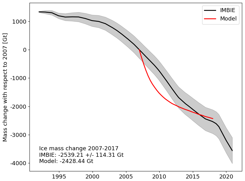
Figure 2 Greenland ice sheet total ice mass change during the calibration period (2007–2017). The model results (red) are shown next to the Ice Sheet Mass Balance Intercomparison Exercise (IMBIE) estimate (black, Otosaka et al., 2023) and uncertainty range (shaded grey) for comparison.

The goal of this calibration run is to calibrate the calving scheme to be used in our transient simulations such that the transient tendency of the ice sheet matches recent observations. We use the von Mises calving parameterization from Morlighem et al. (2016), where the calving rate is set as a fraction of the ice flow speed at the terminus depending on the local stress state. When local tensile stress is above a stress threshold, σ_max, the calving rate exceeds the local speed of ice flow, and the terminus retreats overall due to calving. We set the calving rate to zero if the bedrock is above sea level. We calibrate σ_max on a glacier-by-glacier basis, and we use two observational constraints for the calibration. First, we adjust σ_max at each marine-terminating glacier so that the simulated terminus retreats match the observed retreats along flowlines from Wood et al. (2021) over the calibration period. We use the same set of tunable glaciers with sufficiently well-constrained bathymetry as the method developed by Choi et al. (2021), corresponding to the 148 glaciers where dynamic ice front motion is simulated, driven by calving rates and frontal melting rates (Eqs. 2–3). For glaciers with an ice shelf in northern Greenland, we assume that σ_max of floating ice is 30 % of its value for upstream grounded ice, following Åkesson et al. (2022). As a second metric for our calibration, we use the total GrIS mass loss over 2007–2017 from IMBIE (Otosaka et al., 2023), which amounts to 2539±114 Gt. As shown by Goelzer et al. (2020), most ice sheet models underestimate Greenland mass loss over the recent historical period. Here, in our model calibration, we prioritize matching the observed total mass loss over matching individual glacier retreat rates. Based on our two observational constraints, we establish a simple calibration framework: we target 2007–2017 GrIS mass loss within observational uncertainties, under the constraint that the simulated retreat values of the 148 marine glaciers are within 1 km of the observed retreat values. All calibration occurs by modifying σ_max at marine-terminating glaciers to match both constraints at individual glaciers and the whole ice sheet mass balance.

Figure 2 shows the total ice sheet mass change record from IMBIE (Otosaka et al., 2023), which is compared with the modeled mass loss from our calibration run. The total modeled 2007–2017 mass change agrees with the observational record within uncertainty ranges, even though the modeled mass loss rate is over- and underestimated in the early and later years of the calibration period, respectively. Figure G1 shows a comparison of thickness change over the calibration period with observations, showing generally good agreement, particularly near the ice sheet margins, with modeled thickening in the ice sheet interior slightly higher than in the observations.

This departure from the IMBIE observations of ice sheet is an unavoidable product of having a relatively short calibration period (11 years) in comparison to the natural response time of glacier termini (multi-decadal and longer timescales; Robel et al., 2018). Inaccuracies in the 2007 ice sheet state, which is derived from a mass-conserving data assimilation scheme (Morlighem et al., 2017), transiently adjust to the stress balance approximation and to the assumption of the von Mises calving parameterization with calibrated values of σ_max at all glaciers. These imperfect initial conditions and model physics combine to cause the temporary departure from the observed mass loss trajectory.

Figure 3 compares the observed and modeled 2007–2017 retreat rates at the 148 marine glaciers subject to calibration of σ_max. Our calibration procedure yields a coefficient of determination (R²) of 0.60 and root mean square error of 1.6 km, where these performance metrics are computed over the entire glacier population. While we are generally able to meet our constraint of simulated calving front retreats within 1 km of the observations, it is apparent from the RMSE greater than 1 km that we overestimate the retreat of 79° North in northeastern Greenland and underestimate the retreat of Sermeq Kujalleq (“SK”, previously known by its Danish name Jakobshavn Isbræ). Prior studies have indicated that 79° North may be vulnerable to large retreats in the near future (Choi et al., 2017) and during the Holocene (Roberts et al., 2024). In our calibration run, this sensitivity of 79° North results from the high sensitivity of the von Mises calving parameterization: this glacier exhibits a threshold-like behavior as it either retreats or advances excessively during calibration for any σ_max value. Our aim in using this calibration procedure is to approximate the first-order tendency of the ice sheet and glacier termini in 2017 using currently available best practices (Choi et al., 2021), in the absence of existing ice sheet reanalysis products similar to those that exist for the atmosphere and ocean. We discuss these challenges for future work on the calibration procedure further in Sect. 4.

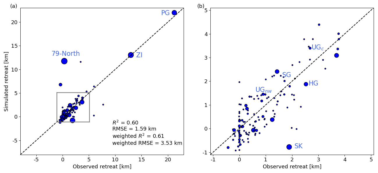
Figure 3 (a) Retreat of the 148 calibrated marine glaciers during the calibration period (2007–2017), where the area of each circle is proportional to the catchment size of the glacier it represents. The performance statistics coefficient of determination (R²) and root mean square error (RMSE) are provided unweighted and weighted by the glacier catchment size. Positive retreat indicates retreat; negative retreat indicates advance. (b) Zoomed-in version of the grey square box shown in (a). Glaciers discussed in the main text are identified, where PG – Petermann Glacier, ZI – Zachariae Isstrom, SK – Sermeq Kujalleq, UG – Upernavik Glacier, SG – Steenstrup Glacier, and HG – Humboldt Glacier. Note that we identify the two main branches of UG: northwestern (UG_nw) and central (UG_c). See Fig. 7a for glacier locations.

2.5 Transient runs 2018–2203

We use our statistical models of processed climatic forcing and calibrated ice sheet model configuration to perform long-term simulations of the GrIS. Using StISSM, we perform several ensemble experiments, as detailed in this section (and listed in Table 1). All simulations start from 2018, i.e., from the final state of the calibration run, and run until 2203. This simulation period is chosen to align with availability of climate forcing from AWI-ESM simulations (maximizing the length of the simulation rather than ending in 2200). We run two deterministic simulations for each of the scenarios considered, applying the mean climate forcing (pre-2000 control and RCP8.5 emissions scenario) but no internal climate variability. All other simulations include stochastically generated climatic forcing calibrated to the long-term outputs from AWI-ESM and dEBM, as detailed in Sect. 2.1 and 2.2.

2.5.1 Pre-2000 control

In order to compare the influence of natural variability versus forced trends on the GrIS, we perform a control ensemble (indicated hereafter by the term CTRL) with stationary forcing from the AWI-ESM pre-industrial climate. In other words, CTRL ensembles assume no trend in SMB, runoff, or ocean thermal forcing: the mean state, covariance matrix, and internal climate variability statistics are held constant to their 1850–1999 levels. Note that the pre-2000 climate conditions are applied immediately at the end of the calibration run, which induces an abrupt but low-magnitude change towards a cooler climate at the start of the transient simulations (Fig. F1). All ensemble members share the same forcing statistics. However, they differ by different random realizations of the internal variability component in the climate forcing throughout the simulation. The resulting large pre-2000 control ensemble (CTRL-LE) consists of 100 member simulations.

2.5.2 High-emissions scenario (RCP8.5)

To quantify the relative importance of forced trends in mean climate relative to internal variability, we perform an ensemble with changing mean climate forcing following the high-emission RCP8.5 scenario simulation of AWI-ESM (indicated hereafter by the term WARM). As described in Sect. 2.3.1, we fit piecewise-linear trends separately for each glacier catchment for TF, SMB, and runoff forcings with breakpoints in 2000, 2050, and 2100. The changing amplitude of climate variability in this forced climate model simulation (Fig. 1) also requires us to specify a different covariance matrix for each of these periods (see Appendix A). The resulting large RCP8.5 ensemble (WARM-LE) consists of 100 member simulations.

We briefly note that our choice of the RCP8.5 high-emissions scenario is mainly motivated by expediency, with availability of long-running climate model simulations, and easy comparison to other ice sheet model intercomparison projects. The two scenarios considered (CTRL and WARM) are meant to be end members of a broad range of potential future emissions scenarios. Future work could further investigate this question by running large ensembles for other emissions scenarios and other global climate models.

2.5.3 Small ensembles

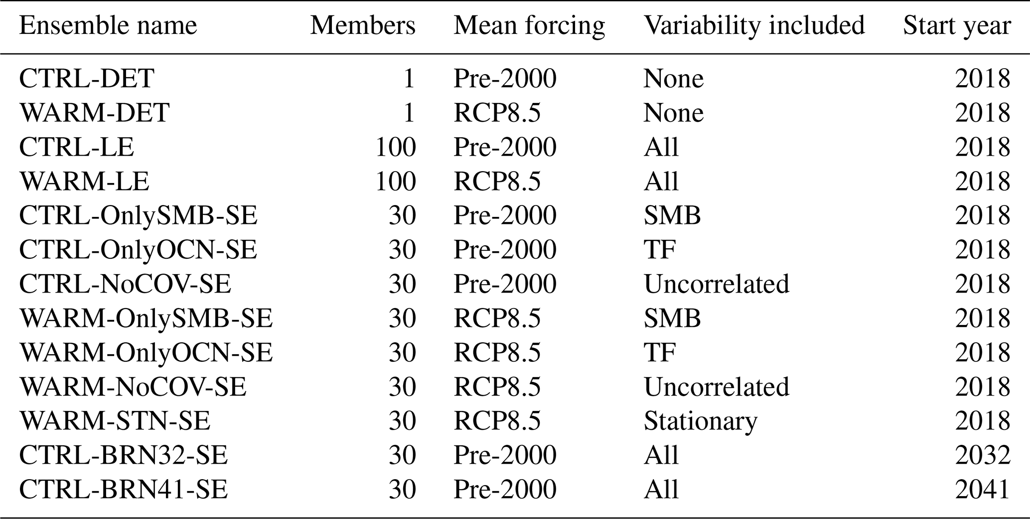
To diagnose the drivers of variability in the simulated GrIS mass change, we perform several additional smaller sub-ensembles with 30 members each, both for the WARM and the CTRL forcings (detailed in Table 1). Specifically, we perform stochastic ensembles with variability only in SMB (OnlySMB-SE), variability only in ocean TF (OnlyOCN-SE), and with variability in all variables but zero covariance between all variables and catchments (NoCOV-SE). The NoCOV-SE applies a diagonal covariance matrix Σ, i.e., without any correlation between different variables and different catchments, but with the magnitude of variability on the main diagonal identical to that of the corresponding full ensemble. For the WARM ensemble only, we also perform an additional small ensemble (WARM-STN-SE), where the covariance matrix does not change in time and is fixed to the covariance matrix of the 2000–2050 period; i.e., the internal climate variability is stationary. This eliminates the increase in amplitude of climate forcing variability in WARM, but the deterministic trend of WARM-STN-SE is identical to the WARM scenario. For the CTRL ensemble, we also performed two additional sets of small “branched” ensembles, which were initialized from a single simulation from the large ensemble in 2032 and 2041 (CTRL-BRN32-SE and CTRL-BRN41-SE, respectively). These small ensembles are designed to elucidate the role of particular events within the simulations in generating ensemble spread, as becomes clear in Sect. 3.

Table 1 List of ensembles of model experiments discussed in this study, with details on ensemble differences. In the column “Variability included”, “All” refers to SMB, runoff, TF, and the correlation between these three variables across Greenland catchments.

3 Results

The aim of this study is to investigate the role of internal climate variability in driving mass change from the GrIS in the future. As a point of comparison, we run two deterministic simulations (CTRL-DET and WARM-DET) applying the mean climate forcing for the CTRL and WARM scenarios but omitting temporal variability in climate forcing. Figure 4a shows the evolution of ice mass for these two simulations as dashed dark blue and dark red lines, respectively. The first 30 years of ice sheet evolution in both deterministic simulations is very similar, indicating that the early evolution is likely driven by a combination of the ice sheet state in 2018 and the pre-2018 mean climate forcing. During these 30 years of similar evolution, there are two notable sub-decadal periods of rapid ice mass loss common to both deterministic simulations (and all other simulations in this study, as discussed in the next sections). These rapid ice loss events are associated with the rapid retreats of Petermann Glacier (PG) in the 2030s and Zachariae Isstrom (ZI) in the 2040s. The loss of floating ice at PG in the first 15 years of the simulation triggers a rapid retreat over a relatively flat bed, until the calving front reaches a region of prograde bed topography. The simulated evolution of ZI starting in 2018 is the ongoing response to the complete loss of floating ice between 2004 and 2012 (Khan et al., 2022). The subsequent calving front retreat proceeds over several wide bed bumps until the frontal geometry adjusts to a more gradually sloped configuration. Over the course of the deterministic simulations, 50 % and 80 % of all marine-terminating glaciers retreat by more than 1 km in the CTRL and WARM deterministic simulations, respectively. However, slower retreat of smaller glaciers contributes less to the overall ice sheet mass loss rate compared to the cases of PG and ZI.

After ∼2050, the two deterministic simulations diverge. Over the remaining 150 years of the simulation, the CTRL climate forcing causes recovery of approximately half of the ice sheet mass loss from the PG and ZI retreats. In contrast, the WARM deterministic simulation continues to lose mass at a rapid and regular pace, mostly driven by increasingly negative SMB across the ice sheet. The CTRL deterministic simulation contributes to 6.0 cm of sea level rise equivalent in 2100, which reduces to 3.1 cm by the end of the simulation in 2203. Ice loss from the WARM deterministic simulation contributes to an equivalent of 11.5 cm of sea level rise in 2100 and 25.4 cm by the end of the simulation in 2203. Though these simulations are not intended as projections, they do fall well within the general range of other GrIS projections (Goelzer et al., 2020), as discussed in more detail in Sect. 4.

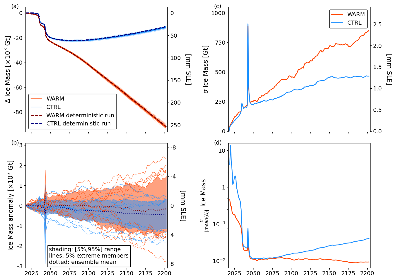
Figure 4 Ice mass evolution in GrISLENS large ensembles. (a) Ice mass change for all ensemble members (colored lines) and deterministic runs (dashed darker lines). (b) Anomaly of ensemble members with respect to their corresponding deterministic run. (c) Ensemble standard deviation (σ) over time. (d) Ensemble standard deviation relative to the ensemble absolute mean mass change. Blue lines and shading are CTRL-LE, and red lines and shading are WARM-LE. In (b), the shading shows the 5 % to 95 % range of the ensemble at any time step, and the lines show the 5 % members with the lowest and largest ice mass at the final time step. On the right y axes, mm SLE denotes millimeters of sea level rise equivalent.

3.1 Control large ensemble (CTRL-LE)

The control large ensemble with pre-2000 climate conditions (CTRL-LE hereafter) includes realistic internal climate forcing variability, represented as stochastic temporal variability in SMB, runoff, and TF in 100 ensemble members. In Fig. 4a, we show the ice mass evolution of all members of CTRL-LE. The main features of the ice mass evolution in the deterministic control run (rapid retreat of PG and ZI and gradual recovery after 2050) occur in all members of CTRL-LE. By 2203, the mean ensemble ice loss is 4 % greater than in the deterministic simulation. This difference is just 1 standard deviation of the ensemble final mass change from the ensemble median, and 17 members have less ice loss than the deterministic run. Thus, while this difference from the deterministic run may be suggestive of potential noise-induced drift in the stochastic ensemble (Tsai et al., 2017; Hoffman et al., 2019; Robel et al., 2024), it is not large enough to be statistically significant (i.e., differences of this magnitude or larger occur by chance in 17 % of ensemble members). We disentangle the mechanisms of this drift more fully in Sect. 3.3 with comparison to small-ensemble experiments.

Figure 4b shows the ice mass evolution of each member as an anomaly with respect to the deterministic run. It is clear that most of the CTRL-LE ice mass anomalies are negative, confirming the 4 % larger mass loss from the CTRL-LE ensemble mean compared to its corresponding deterministic run. Another feature apparent in Fig. 4b is that the members at the lowest and highest ends of the ensemble mass loss at the final time step (lines) mostly exhibit low-end and high-end ice mass anomalies throughout the simulation. That is, their ice mass deviation from the ensemble mean is caused by climatic perturbations early in the simulation that produce a response which persists and continues growing over the simulation period. This persistence is characteristic of dynamical systems involving long-response timescales and positive feedback processes. In our simulations, this includes the SMB–elevation feedback and the dynamic thinning propagating upstream following marine glacier retreat.

Figure 4c shows the standard deviation between ensemble members of CTRL-LE (blue line), hereafter referred to as “ensemble spread”. The CTRL-LE spread increases until 2150, before leveling off. The ensemble spread temporarily increases by 25 % for the rapid retreat of PG and by almost 300 % during the rapid retreat of ZI. In both cases, the ensemble spread quickly returns to the trajectory of gradual increase once retreat has occurred in all ensemble members. At the end of the simulation period, the ensemble spread amounts to 1.3 mm of equivalent uncertainty in sea level contribution and 2.5 mm uncertainty at its peak during the retreat of ZI. To put this ensemble spread in context, in Fig. 4d we also show the ratio of the ensemble spread to the ensemble mean ice loss. This ratio represents the relative importance of uncertainty through the simulation. We note that the denominator in this ratio starts near zero and so should be interpreted with caution, though it does help us to understand the relative importance of ensemble spread as compared to ensemble mean change. Over the first 20 years of the simulation period, ensemble spread accounts for 10 %–300 % of the ensemble mean mass loss. Once ZI and PG retreat, the ensemble spread never exceeds 5 % of the mean ice loss. However, this relative uncertainty grows steadily from 2075 as a result of the ice mass recovery of the ensemble mean (Fig. 4a). These results indicate that in the near future (decades), climate variability plays an important role in the progress of Greenland ice mass loss. Once the total mass loss ramps up, climate variability is a less important source of uncertainty on the ice sheet scale compared to the total ice loss and scenario uncertainty (i.e., the difference between CTRL-LE and WARM-LE, as seen in Fig. 4a).

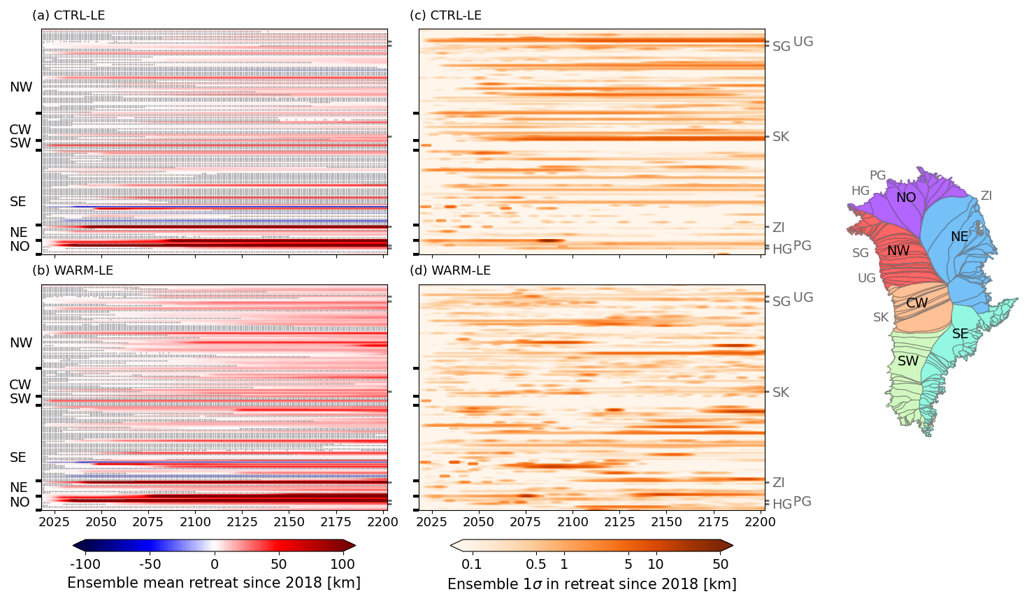
Figure 5 Cumulative retreat of terminus position since the transient simulation start date (2018) for each marine-terminating glacier in Greenland: a retreat of x km in year y indicates that the terminus has retreated by x km between 2018 and y. Glaciers are grouped by regions as follows: NO – north, NE – northeast, SE – southeast, SW – southwest, CW – central west, and NW – northwest (see map on the right). (a–b) Ensemble mean of retreat extent [km] in (a) CTRL-LE and (b) WARM-LE. Red indicates retreat; blue indicates advance. (c–d) Ensemble spread of retreat extent [km] in (c) CTRL-LE and (d) WARM-LE. In (a) and (b), the grey hatching denotes non-significant retreat/advance, where significance is evaluated as agreement on the sign of retreat between 95 % of ensemble members. Note the logarithmic color bar in (c) and (d). The individual glaciers identified on the right y axes are PG – Petermann Glacier, ZI – Zachariae Isstrom, SK – Sermeq Kujalleq, UG – Upernavik Glacier, SG – Steenstrup Glacier, and HG – Humboldt Glacier (see locations on the map on the right).

Figure 5 shows the mean (panel a) and spread (panel c) of terminus retreat at all marine-terminating glaciers where calving and melt forcing occur in CTRL-LE. The retreat of some glaciers is highly uncertain, with some ensemble members retreating tens of kilometers and others not at all. For most glaciers, the ensemble spread in Fig. 5c–d remains approximately constant after 2050, indicating that most of the uncertainty stems from the internal climate variability causing retreats in some ensemble members early in the simulations. Figure 6 shows flowline thickness profiles for all CTRL-LE ensemble members at selected glaciers and times. PG (Fig. 6a) and ZI (Fig. 6b) experience the most uncertainty in the simulated terminus position in the midst of rapid retreat, with ensemble members differing by up to 10 km, before converging following the main period of retreat. In contrast, at other glaciers, including the Upernavik and Steenstrup glaciers (Fig. 6c, d), the extent of retreat depends strongly on the details of climate variability. The result is that individual ensemble members undergo retreats that differ by up to 10 km in extent, and this difference can persist until the end of the simulation period. For these glaciers, there are a discrete number of positions where the front persists in different ensemble members, punctuated by rapid retreats on sub-decadal timescales between positions. This is a known behavior of marine-terminating glaciers retreating over bed topography with many local peaks of varying height (Robel et al., 2022). PG and ZI are among the largest catchments in Greenland, so when retreats occur over a sufficiently short time period (less than a decade) and across all ensemble members, small differences in the timing of retreat onset cause the large increase in total ice sheet mass ensemble spread (Fig. 4c). Other glaciers are either sufficiently small or retreat relatively slowly, and so even when there are persistent and large differences in the extent of retreat (e.g., at Upernavik and Steenstrup), they have a limited impact on the ensemble mean or spread.

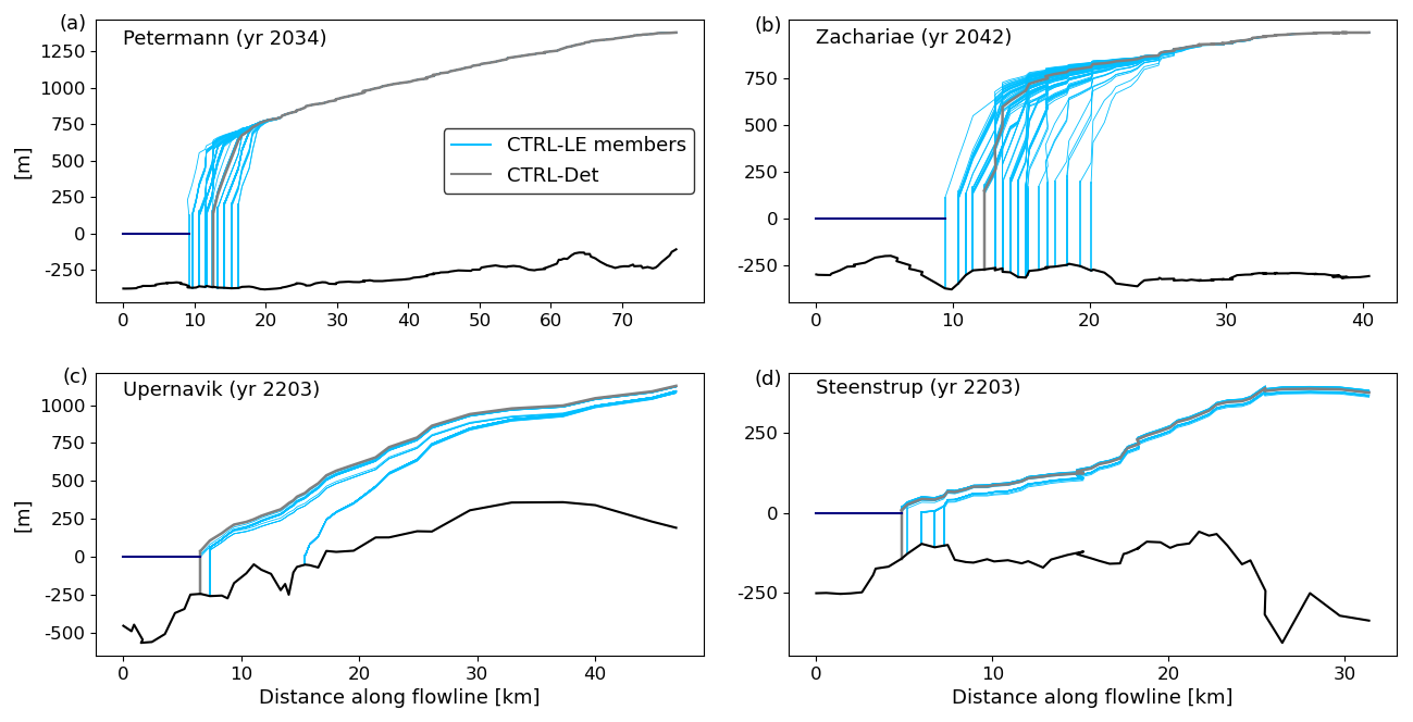
Figure 6 Along-flow profiles of ensemble near-terminus ice thickness for four glaciers at various points during the simulation period in CTRL-LE (blue profiles) and CTRL-Det (grey profiles). (a) Petermann Glacier (year 2034). (b) Zachariae Isstrom (year 2042). (c) Upernavik Glacier (year 2203). (d) Steenstrup Glacier (year 2203). All 100 ensemble members of CTRL-LE are included in the plots, and each profile corresponds to a single ensemble member. See Fig. 7a for glacier locations.

Thickness changes in CTRL-LE are mapped in Fig. 7, with the top row showing ensemble mean thickness changes in 2050, 2100, and 2203; the middle row the difference with respect to the deterministic simulation; and the bottom row the corresponding ensemble spread. Before 2100, a dynamic thinning of hundreds of meters occurs far upstream of retreating termini at PG, ZI, and other marine-terminating glaciers in western and southeastern Greenland. Gradual thickening of tens of meters occurs across the ice sheet interior, mainly after 2100. This progression largely explains the ice mass evolution in Fig. 4a, with dynamic thinning driving most ice loss early in the simulation and positive SMB in the ice sheet interior causing thickening later.

During the retreats of PG and ZI, slight differences in retreat timing between ensemble members cause tens to hundreds of meters of uncertainty in the upstream-propagating wave of dynamic thinning (e.g., at ZI in Fig. 7g), which quickly dissipates once all ensemble members have retreated (Fig. 7h, i). In contrast, at glaciers where uncertainty in retreat extent persists (e.g., Upernavik Glacier), there remains hundreds of meters of uncertainty in dynamic thinning, which gradually spreads upstream and into adjacent catchments over the simulation period (Fig. 7h, i). SK does not begin to undergo retreat until after 2050 in CTRL-LE, though differences among ensemble members in retreat onset timing produce large uncertainties in thinning during the middle part of the simulation period (2070–2150; see Fig. 7h). By the end of the simulation, SK has retreated in all ensemble members, and thinning uncertainty has largely dissipated (Fig. 7i). Across glacier catchments in the southern half of Greenland, SMB variability drives gradually increasing uncertainties in thickness evolution over large areas; it generally remains an order of magnitude lower than that of retreating glaciers in western Greenland (Fig. 7g, h, i). The relative importance of ocean-driven dynamic thinning and SMB variability is discussed in further detail in Sect. 3.3. Differences in ice thickness between the CTRL-LE mean and the deterministic simulation are mostly small (Fig. 7d, e, f). The most pronounced differences appear for outlet glaciers in western and southeastern Greenland. The stronger ice loss in CTRL-LE than in the deterministic simulation (see Fig. 4a) can mostly be attributed to localized enhanced thinning at two large outlet glaciers (Fig.7f).

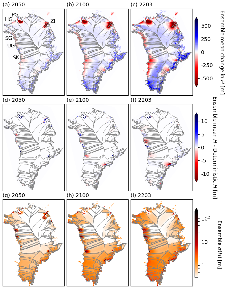
Figure 7 Ice thickness (H) in CTRL-LE. Top row: ensemble mean change in H between 2018 and (a) 2050, (b) 2100, and (c) 2203. Middle row: difference in H between ensemble mean and the deterministic simulation in (d) 2050, (e) 2100, and (f) 2203. Bottom row: ensemble spread (σ(H)) in (g) 2050, (h) 2100, and (i) 2203. Note the different color scales in (a)–(c) and (d)–(f), as well as the logarithmic color scale in (g)–(i). Color scales are identical to those in Fig. 8. Glacier locations are shown in (a) for PG – Petermann Glacier, ZI – Zachariae Isstrom, SK – Sermeq Kujalleq, UG – Upernavik Glacier, SG – Steenstrup Glacier, and HG – Humboldt Glacier.

3.2 RCP8.5 large ensemble (WARM-LE)

The RCP8.5 large ensemble (hereafter WARM-LE) is initialized identically to CTRL-LE, but the statistics of the climate forcing evolve over time, leading to increasingly intense surface melt and ocean thermal forcing over the course of the simulation period. WARM-LE is meant to be a point of comparison with CTRL-LE. First, we determine how the ice sheet responds differently to changes in the mean climate as compared to internal climate variability. Second, we analyze how the response to internal variability may differ under different background climatic states. We note briefly that RCP8.5 is a high-end-member emissions scenario, and the following results should be interpreted as a model experiment, not a projection.

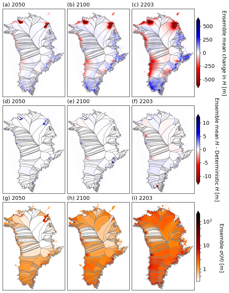
Figure 8 Ice thickness (H) in WARM-LE. Top row: ensemble mean change in H between 2017 and (a) 2050, (b) 2100, and (c) 2203. Middle row: difference in H between ensemble mean and the deterministic simulation in (d) 2050, (e) 2100, and (f) 2203. Bottom row: ensemble spread (σ(H)) in (g) 2050, (h) 2100, and (i) 2203. Note the different color scales in (a)–(c) and (d)–(f), as well as the logarithmic color scale in (g)–(i). Color scales are identical to those in Fig. 7.

The evolution of the WARM-LE ice mass (Fig. 4, red lines) is qualitatively similar to that of the deterministic simulation (dashed dark red line). At the end of the simulation period, the spread in WARM-LE ice mass loss accounts for 2.4 mm of equivalent uncertainty in sea level rise as compared to the ensemble mean ice mass loss equivalent to 255 mm sea level rise. Prior to 2050, the WARM-LE mean and spread (Fig. 4a, c) track very closely to CTRL-LE, as the ice sheet response is dominated by retreats of PG and ZI. The two spikes in ensemble spread associated with these retreats occur in the same model years in CTRL-LE and WARM-LE. These similarities confirm that the behavior early in simulations is largely caused by a combination of the initial ice sheet state and the ice sheet disequilibrium with the climate at the beginning of the simulation. Evolving mean climate forcing (Fig. F1) appears to play little role in these first few decades of the ensemble. Prior to the retreat of PG, the ensemble mean ice mass loss is sufficiently higher in WARM-LE than in CTRL-LE such that the ratio of ensemble spread to mean ice loss (Fig. 4d) is generally lower, though still substantial (10 %–30 %) in the first ∼20 years of the simulation period. This effect is also evident on longer timescales, where all ensemble members have a common ice sheet response to increasingly intense surface melt and ocean thermal forcing that dominates differences between ensemble members caused by internal climate variability. Finally, Fig. 4b shows the anomaly in each WARM-LE member with respect to the deterministic WARM run. Similarly to CTRL-LE, there is a pronounced persistence of early stochastic perturbations to the ice sheet mass throughout the entire simulation period. As a result, the members with the most extreme final ice mass totals are generally characterized by trajectories being at the lower or upper end of the ensemble already in the first few decades or even years (Fig. 4b).

Figure 8 shows the evolution of ensemble mean and spread in ice thickness for WARM-LE, and Fig. 9 shows the difference between WARM-LE and CTRL-LE in terms of ensemble mean and spread in thickness at the end of the simulation period. In the first few decades of the simulation period, several marine-terminating glaciers in western Greenland undergo rapid retreat and dynamic thinning (Fig. 8a and glaciers in the CW and NW regions in Fig. 5c). One major difference from CTRL-LE is that these retreats are more uniform across ensemble members (compare glaciers in the CW and NW regions in Fig. 5b and d). This results in persistently less ensemble spread in near-margin thinning in these western Greenland catchments (Fig. 9b). In contrast, throughout the simulation period, there is greater ensemble spread in the catchment-wide thickness across most of the Greenland interior. Such a catchment-wide response is caused by variability in SMB. An increase in the amplitude of SMB variability (discussed in more detail in the next section) is already apparent early in the simulation period and continues to drive growing spread in thickness until the end of the simulation period. The greater areal extent of this SMB-driven increase in ensemble spread drives the overall greater spread in ice mass in the later part of the WARM-LE simulation period (Fig. 4b).

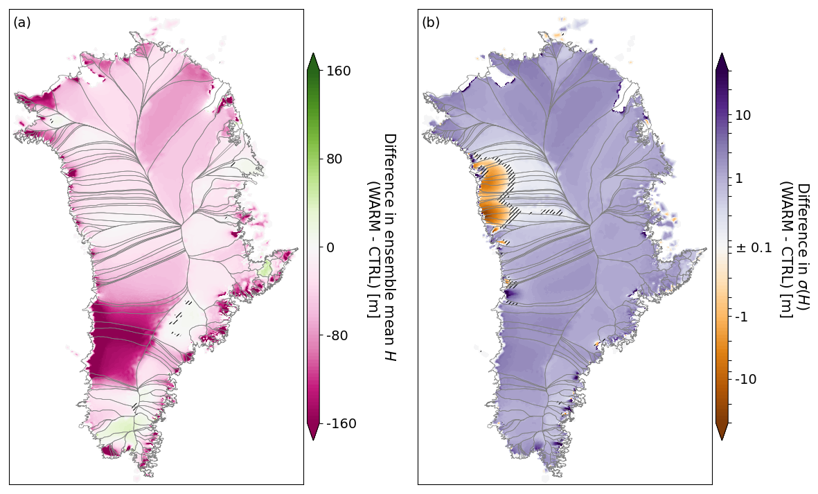
Figure 9 Difference in ice thickness change in 2203 between CTRL-LE and WARM-LE in terms of (a) ensemble mean (pink is greater ensemble mean thinning in WARM-LE) and (b) ensemble spread (σ(H), blue is more ensemble spread in WARM-LE). Note the pseudo-logarithmic color scale in (b). Hatching denotes non-significant differences, evaluated with a 300-sample bootstrap procedure and controlled for a false discovery rate of 0.05 (see Appendix H).

After 2050, ice sheet evolution in WARM-LE departs more strongly from CTRL-LE (compare Figs. 8b, c and 7b, c, and see Fig. 9a). At this point in the simulation period, the mean climate forcing has strongly diverged between the two large ensembles (Fig. F1), and the ice sheet has had sufficient time to respond to the different climate forcing. SMB has decreased enough to cause thinning across almost the entire ice sheet interior except for some land-terminating glacier catchments in far southern Greenland (Fig. 8b, c). Marine-terminating glaciers across the whole ice sheet experience more extensive retreat and more intense dynamic thinning, particularly between 2100–2200 (Fig. 8c). WARM-LE spread in ice thickness is higher than CTRL-LE spread across most of the ice margins (Fig. 9b), indicating that retreat and the resultant dynamic thinning are variable across ensemble members, driven by variability in mean surface melt in the ablation zone and ocean melt at calving fronts. In all WARM-LE simulations, SK undergoes an early retreat that does not occur until later in CTRL-LE. However, at the end of our simulation period, the strong ocean forcing has driven a second retreat at SK, which drives an increase in ensemble spread. It may be that given further simulation time, this could grow to become a substantial source of ensemble spread. WARM-LE spread in ice thickness is also higher than CTRL-LE across the ice sheet interior, though to a lesser extent than at the margins, likely resulting from the increasing amplitude of SMB variability through the simulation period. Finally, we note that for WARM-LE, the differences between the ensemble mean and the corresponding deterministic simulation are also small. However, the differences in 2203 at outlet glaciers are notably smaller than those for CTRL-LE (compare Figs. 8f and 7f). In contrast, differences are more extensive across the ice sheet interior but still of low magnitude (<5 m, Fig. 8f).

3.3 Small ensembles

Our explicitly stochastic approach to representing internal variability in climate forcing in ice sheet simulations allows us to systemically remove or modify different sources of climate variability in our simulations. To determine which aspects of climate variability are the primary contributors to the leading-order statistical moments and certain behaviors in the large ensembles discussed in the prior sections, we analyze a series of “small” ensembles (described in Sect. 2.5.3). For both CTRL and WARM climate forcings, this includes OnlySMB-SE, OnlyOCN-SE, and NoCOV-SE. In addition, the small ensembles include WARM-STN-SE, i.e., the WARM scenario with a fixed covariance matrix, and the two branched ensembles, CTRL-BRN32-SE and CTRL-BRN41-SE, which branch from the CTRL scenario in 2032 and 2041. In light of Fig. 4, the purpose of the latter two small ensembles is clear: by branching the ensemble in these years, we eliminate all pre-existing ensemble spread in order to understand the role of the retreats of PG (starting in 2033 in most LE members) and ZI (starting in 2042 in most LE members) in generating ensemble spread.

3.3.1 Control small ensembles

In Fig. 10a, we show the distribution of ice mass change across the large and small ensembles with CTRL climate forcing. In general, we find that all aspects of variability contribute somewhat to the large-ensemble spread, including the SMB, ocean, and covariance structure of the climate forcing. Omitting covariance between SMB and ocean thermal forcing variability and between catchments (CTRL-NoCOV-SE; dark red data in Fig. 10a) reduces ensemble spread by 44 %. Applying SMB variability only (CTRL-OnlySMB-SE; orange data in Fig. 10a) reduces ensemble spread by 36 % and shifts the ensemble towards less ice mass loss, with the mean and median being approximately equivalent to the 75th percentile in CTRL-LE. Applying ocean variability only (CTRL-OnlyOCN-SE; blue data in Fig. 10a) reduces ensemble spread by 61 % without a substantial shift in the mean.

Figure 10a also shows that at the end of the simulation period, CTRL-LE (green data) is skewed towards more mass loss (see also Fig. E1 in Appendix E). This is indicated visually by a “long tail” of five ensemble members, in which there is much more mass loss than for the equivalent ensemble members on the other end of the distribution (less mass loss). While prior studies (Robel et al., 2019) have indicated that such high-end skew in simulations of mass loss may occur during periods of rapid retreat, there are no ongoing rapid retreats of large catchments in CTRL-LE at the end of the simulation period. The time-dependent calculation of skewness (Fig. E1 in Appendix E) indicates that this persistent skewness only arises in the last 50 years of the simulation period. Since none of the small ensembles have such skew, we can conclude that correlation between the ocean and SMB variability is the cause of this skew, as this is the only factor omitted from all three ensembles (CTRL-NoOCN-SE and CTRL-NoSMB-SE implicitly omit these correlations by zeroing out variability in one or another type of variability). However, our small ensembles are too small to robustly attribute skewness on the basis of just a few “outlier” ensemble simulations; thus we leave this possibility as a hypothesis to be further evaluated in future work.

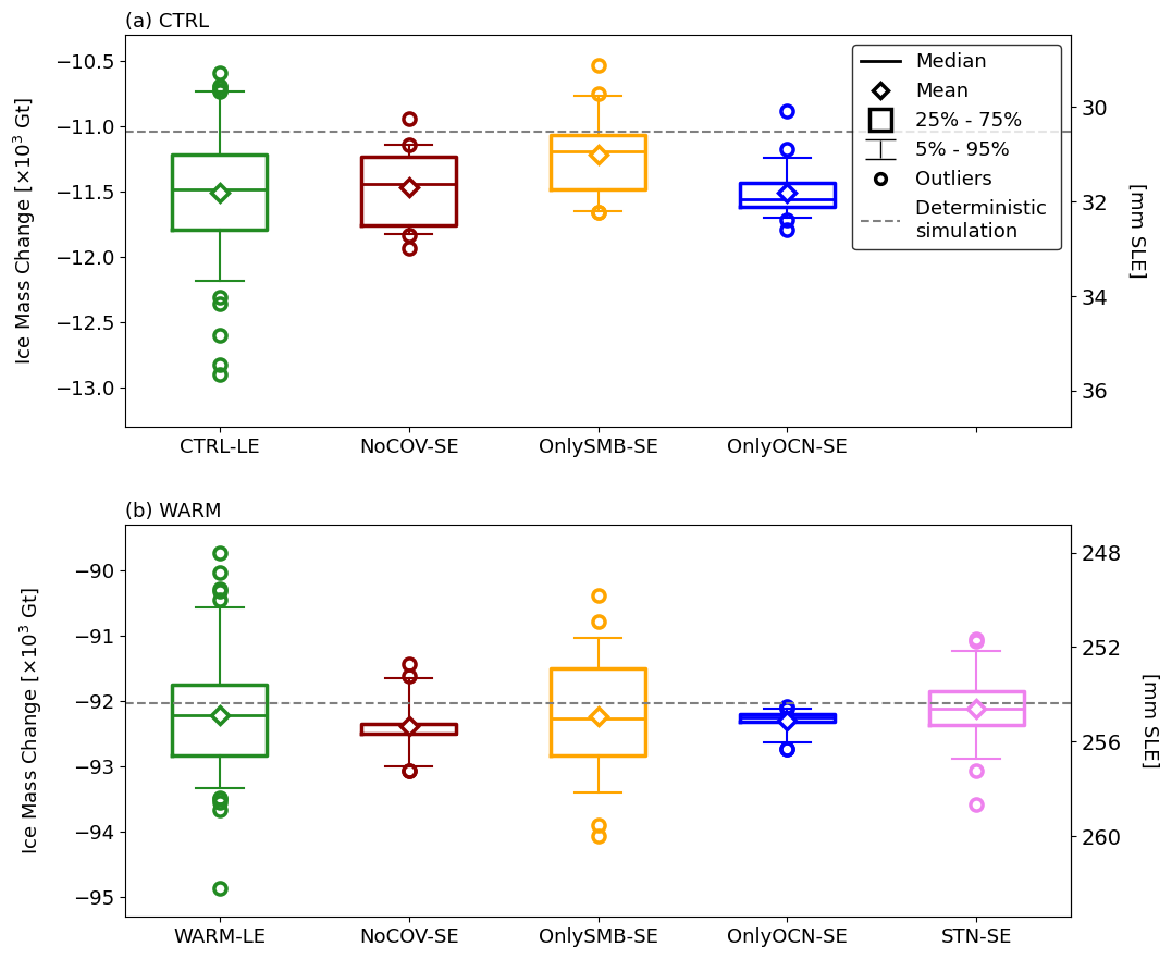
Figure 10 Boxplots showing distribution of ice mass change in the year 2203 in all ensemble members for the (a) CTRL and (b) WARM climate forcings. Shown in (a) are CTRL-LE (green), CTRL-NoCOV-SE (dark red), CTRL-OnlySMB-SE (orange), and CTRL-OnlyOCN-SE (blue). Shown in (b) are WARM-LE (green), WARM-NoCOV-SE (dark red), WARM-OnlySMB-SE (orange), WARM-OnlyOCN-SE (blue), and WARM-STN-SE (violet). Horizontal lines indicate the ensemble median, diamonds ensemble mean, boxes inter-quartile (25 %–75 %) range, whiskers 5 %–95 % range, and circles individual outliers. The dashed horizontal grey lines show the ice mass loss in the corresponding deterministic simulations. On the right y axis, mm SLE denotes millimeters of sea level rise equivalent. Note that the span of the y axis in (a) is exactly half of that in (b).

These small-ensemble results indicate that over the simulation period, the largest drivers of spread in the large ensemble are SMB variability and the spatial covariance between different climate forcing variables and glacier catchments. In Fig. 11a, we show the difference in ensemble spread in ice thickness between CTRL-OnlyOCN-SE and CTRL-OnlySMB-SE for 2203. SMB variability drives most variability in ice thickness over the Greenland interior. This SMB-driven thickness variability is higher by up to 10 times in the south compared to SMB-driven thickness variability in central and northern Greenland. In comparison, ocean variability drives an even higher amplitude of thickness variability over small regions encompassing the dynamic thinning wave from retreat of glaciers, mostly in western Greenland (e.g., Upernavik and SK).

In quantitative terms, we find that less than 10 % of the area of the GrIS is dominated by ocean-driven thickness variability, with thickness variability in the rest of the ice sheet being driven by SMB. However, the higher intensity of ocean-driven thickness variability in these small regions means that ocean variability alone (i.e., CTRL-OnlyOCN-SE) drives 40 % of the mass balance variability for all of Greenland, as simulated in the large ensemble (CTRL-LE).

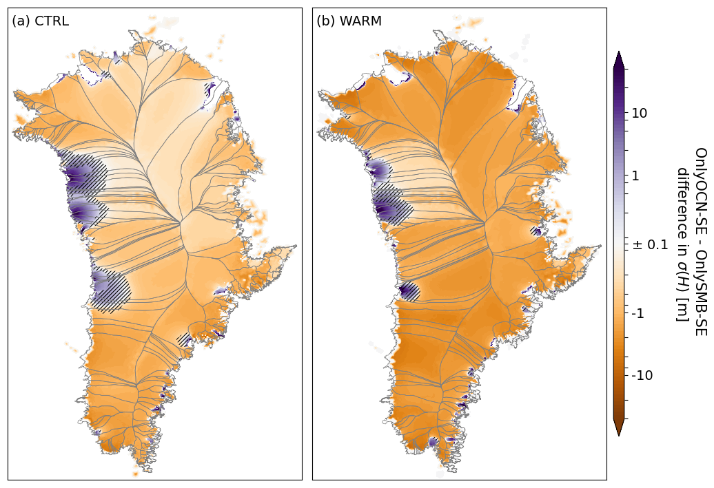
Figure 11 Difference between ensemble spread in ice thickness (σ(H)) in 2203 in OnlyOCN-SE versus OnlySMB-SE for (a) CTRL climate forcing and (b) WARM climate forcing. Greater spread in OnlyOCN-SE is indicated by blue, and greater spread in OnlySMB-SE is indicated by orange. Note the pseudo-logarithmic color scale. Hatching denotes non-significant differences, evaluated with a 300-sample bootstrap procedure and controlled for a false discovery rate of 0.05 (see Appendix H).

If the ensemble mean of the ice sheet mass loss were driven entirely by the climate forcing scenario (i.e., the difference between CTRL and WARM), then we should expect no statistically significant difference between the small-ensemble means of CTRL and the CTRL-LE mean, since only the variability in climate forcing is modified in the small ensembles. We use Welch's t test with unequal variances and sample sizes (Welch, 1947) to determine whether the mean ice mass loss of the small ensembles is significantly different from that of the CTRL-LE mean. Indeed, there is no significant difference between CTRL-OnlyOCN-SE and CTRL-NoCOV-SE (p>0.5). However, CTRL-OnlySMB-SE has a shift in the ensemble mean ice loss that is statistically significant ($p<{\mathrm{10}}^{-\mathrm{3}}$), as excluding ocean forcing variability decreases total ice loss. This difference strengthens the hypothesis of noise-induced drift in CTRL-LE compared to the deterministic run (4 % greater mass loss; see Fig. 4a, b), since the deterministic run also lacks ocean variability. This result is consistent with prior work finding that ocean variability drives real drift in the direction of retreat in ice sheet evolution (Verjans et al., 2022; Robel et al., 2024). Since ocean variability drives uncertainty in the onset time of glacier retreat over peaks in bed topography, the model drift here is thus probably entirely caused by noise-induced bifurcations, as described previously by Robel et al. (2024).

3.3.2 Branched small ensembles

As discussed in previous sections, the rapid retreats of PG and ZI play an important role in generating ensemble spread during the period of the retreats. The branched small ensembles (CTRL-BRN32-SE and CTRL-BRN41-SE) allow us to understand the sources and persistence of this retreat-mediated uncertainty. Figure 12 shows the ensemble spread of total ice mass over the simulation period for CTRL-LE (green line), CTRL-BRN32-SE (dark red line), and CTRL-BRN41-SE (orange line). CTRL-BRN32-SE shows a similar increase in ensemble spread during the retreat of PG as compared to CTRL-LE, indicating that most of the ensemble spread generated at PG is related to climate forcing variability during the PG retreat, driving differences in retreat rates. In contrast, when there is less ensemble spread at the onset of ZI retreat, there are much smaller increases in ensemble spread during the ZI retreat. This indicates the importance of retreat onset timing at ZI for determining how much the ensemble spread increases during the retreat. Finally, despite substantial differences in the magnitude of ensemble spread increases during large retreats in the branched small ensembles, the final differences in ensemble spread are similar in magnitude to the differences existing before the retreats simply by starting simulations at a new time. Thus, we conclude that while ensemble spread increases substantially during retreats, this spread does not persist if all ensemble members ultimately undergo the same retreat. This contrasts with the ensemble behavior for glaciers such as Upernavik and Steenstrup, where some members of CTRL-LE and WARM-LE undergo retreat, while others do not. In such cases, uncertainty is likely to be persistent.

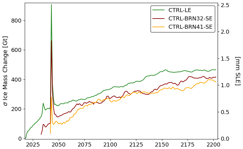
Figure 12 Ensemble spread (σ) in total ice sheet mass change for CTRL-LE (green), CTRL-BRN32-SE (dark red), and CTRL-BRN41-SE (orange). On the right y axis, mm SLE denotes millimeters of sea level rise equivalent.

3.3.3 RCP8.5 small ensembles

By the end of the simulation period, WARM-LE has about twice as much ensemble spread as CTRL-LE, though the drivers of this spread are not qualitatively different (Fig. 10b). When only SMB variability is imposed (OnlySMB-SE, orange data in Fig. 10b), there is no significant change in the ensemble spread (p>0.4 in Levene's test, Levene, 1960). However, omitting spatial covariance in SMB between catchments (NoCOV-SE, dark red in Fig. 10b) or SMB variability entirely (OnlyOCN-SE, blue in Fig. 10b) causes ensemble spread to be significantly reduced (54 % and 81 % reductions, respectively). In WARM-LE, the amplitude of climate forcing variability changes over the simulation period, and we change the prescribed covariance to capture this non-stationarity (e.g., Fig. 1). This is particularly relevant to SMB variability, which is amplified strongly in the AWI-ESM climate model response to the RCP8.5 scenario. As a result, Fig. 11b shows that SMB-driven variability is more pronounced across Greenland than in the CTRL forcing scenario and that areas dominated by ocean-driven variability are more restricted. In WARM-STN-SE, we omit the increasing amplitude of variability in SMB, as well as all other climatic forcings, by keeping the forcing covariance constant in 2000–2050 values over the simulation period. As a result, the ensemble spread in WARM-STN-SE is reduced by 33 % (violet data in Fig. 10b). This difference is a large fraction of the inter-ensemble spread between WARM-LE and CTRL-LE (33 % versus 46 %). To investigate this contribution, Fig. 13 shows the ratio of the interannual SMB variability from dEBM in the last 3 decades of the simulation period to that in the first 3 decades. In most of eastern Greenland and some catchments in central western Greenland, the amplitude of SMB variability is 2–8 times higher in the final decades of the simulation period as compared to the starting decades. No catchment shows any appreciable decrease in SMB variability over this period. The WARM small ensembles thus tell a consistent story: in a strongly warming climate, (1) the full-ensemble spread can be explained by SMB variability alone, and (2) almost $\mathrm{1}/\mathrm{3}$ of ensemble spread in the year 2203 can be attributed to the warming-driven increase in the amplitude of SMB variability over the next 2 centuries.

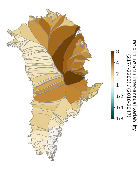
Figure 13 Ratio of amplitude of catchment-averaged SMB interannual variability in dEBM under the RCP8.5 scenario between the last 3 and first 3 decades of our simulations (2174–2203 to 2018–2047). Note that this time-evolving SMB field of dEBM is used to constrain the SMB statistics of the WARM climate forcing.

If there is any drift in the ensemble mean ice loss in WARM-LE, it is not statistically distinguishable from the larger envelope of ensemble spread in this ensemble at the end of the simulation period. In addition, none of the small-ensemble results suggest that a particular variability component causes noise-induced drift, in contrast to the CTRL forcing case (Fig. 10). Furthermore, though there are some outlier ensemble members in WARM-LE, their number is limited, making it difficult to draw conclusions about skewness of ice mass without a larger ensemble (which would be computationally challenging to run within the context of this study).

4 Discussion

The main conclusion of this study is that in the first 2 decades of simulations, climate variability plays an important role in generating uncertainty in the evolution of total ice sheet mass and contribution to sea level rise. Beyond this initial period, internal climate variability quickly diminishes in importance at the ice sheet scale, particularly when compared to uncertainty in future emissions scenarios. This conclusion is derived from a large ice sheet model ensemble constituting the most advanced quantification of the role of climate variability in future GrIS evolution. The modeling experiments described in this study are unprecedented in terms of the resolution of ice sheet model simulations (<1 km at calving fronts), the inclusion of dynamic calving, the size of ensembles, and the correction of stochastic climate variability to match the statistics of the observations.

Our findings are consistent with broader climate modeling results on key variables, such as global and regional trends in temperature and precipitation, where internal variability is a major component of uncertainty in the near future (Lehner et al., 2020). The uncertainty in future GrIS evolution is largely driven by SMB, spatial correlations in SMB, and the increasing amplitude of variability in SMB. Within individual glacier catchments and time periods of the simulation, uncertainties in mass loss can be considerably greater due to ocean variability driving uncertainty in the timing of rapid glacier retreats. This is particularly notable in western Greenland, where individual ensemble members exhibit retreats differing in timing by decades, for example at the SK, Upernavik, and Steenstrup glaciers. This future sensitivity of glaciers in western Greenland to ocean forcing is consistent with a similar sensitivity of recent (1979–2018) glacier retreat to ocean variability in central western and southern Greenland, as shown by Slater and Straneo (2022). They argue that southern and central western Greenland is directly exposed to North Atlantic oceanic variability. Indeed, the amplitudes of both seasonal and interannual variability in our stochastic parameterization of the oceanic thermal forcing, derived based on a high-resolution ocean reanalysis product (Nguyen et al., 2012), are the highest in southern and western Greenland (Verjans et al., 2023).

4.1 Comparison to prior large-ensemble studies

A previous study by Tsai et al. (2017) found that ensemble mean ice sheet response to the coupled CESM large ensemble is about 12 cm sea level rise equivalent in 2100, which is very similar to our simulated WARM-LE ice loss. However, they find an ensemble spread at this time of ∼22 mm, which is approximately 1 order of magnitude more spread than our value of 1.3 mm in 2100 in WARM-LE. The study of Tsai et al. (2017) is the closest point of comparison for GrISLENS. Their study used two large ensembles of a global climate model to force an ice sheet model until 2100 under an RCP8.5 scenario in order to quantify the role of internal climate variability in driving uncertainty in future Greenland ice loss. The mean climate forcing was bias corrected to modern observations, but the climate variability was purely as predicted by their global climate model, in contrast to our methods for generating climate variability, which are corrected to observed variability (Verjans et al., 2023; Ultee et al., 2024). Additionally, the computational constraints of running climate model large ensembles requires a coarse horizontal resolution: 3.75° for the ocean–atmosphere coupled LE used by Tsai et al. (2017) and 1° for the model in Tsai et al. (2017) or about 3 and 10 grid points across Greenland, respectively. Similarly, the ice sheet model for their study was run at 20 km resolution, which is too coarse to explicitly resolve most Greenland outlet glaciers. Their ice sheet model was also initialized at a steady state in 2000, which does not capture the strong Greenland mass loss trend, estimated to have started earlier in the 20th century (Mouginot et al., 2019).

Both GrISLENS and Tsai et al. (2017) attribute most of the simulated ensemble spread to SMB variability. Though it is challenging to definitively attribute the cause of these starkly different ensemble spreads, the most likely explanation is the coarse resolution of the climate model forcing in Tsai et al. (2017) (∼400 km for the coupled LE forcing compared to 5 km for dEBM; see Sect. 2.2.2). Such a resolution introduces spurious spatial correlation between catchments in SMB, which, as we have shown, plays an important role in driving ensemble spread under warming. Indeed, we find that accounting for realistic inter-catchment correlation in WARM-LE more than doubles the ensemble spread compared to assuming uncorrelated catchments. It is therefore unsurprising that representing SMB over Greenland as only ∼10 grid points can cause a further 10-fold increase in ensemble spread, as this approach assumes almost perfect correlation across large portions of the entire ice sheet.

Tsai et al. (2017) also find substantial evidence of drift between simulations forced with and without internal climate variability, even under strong emissions forcing, which they attribute to the use of a positive degree day (PDD) scheme for calculating SMB. This is consistent with recent work, showing that nonlinearities in PDD schemes (Lauritzen et al., 2023) or other ice sheet processes (Robel et al., 2024) can lead to noise-induced drift, particularly in models starting from a deterministic steady state. We directly generate Gaussian stochastic variability in SMB (as indicated by observations; Ultee et al., 2024) and start from a more realistic out-of-balance initial ice sheet state. These factors are consistent with the absence of statistically significant drift in WARM-LE.

Aschwanden et al. (2019) provide another useful point of comparison to GrISLENS. In their study, parameters for ice flow and forcing parameterizations were perturbed over 500 ensemble members with an ice sheet model of sufficiently high resolution (1 km) over Greenland to resolve individual outlet glaciers. They found consistently much greater mass loss compared to WARM-LE, with a median sea level contribution of 22 cm in 2100 (compared to 11 cm in WARM-LE) and 103 cm in 2200 (compared to 25 cm in WARM-LE). Ensemble spread in Aschwanden et al. (2019) is also much greater than in WARM-LE, with a standard deviation of 10 cm SLE in 2100 and 50 cm SLE in 2200, about 2 orders of magnitude greater than the WARM-LE ensemble spread. Later work to calibrate these ensembles using observations reduced the median and spread of their ensemble (Aschwanden and Brinkerhoff, 2022), but the broader higher sensitivity and spread compared to WARM-LE remain. Decomposing the parametric uncertainty quantified in their ensemble using Sobol indices, they find that in 2100, uncertainty in ice flow and surface melt parameters contributes the most to uncertainty in total ice sheet mass loss. In 2200 and beyond, uncertainty in the sensitivity of mean atmospheric temperatures to emissions forcing (i.e., climate sensitivity) dominates uncertainty in total ice sheet mass loss. Consistent with our study, they find that uncertainty in ocean forcing plays a relatively minor role in driving uncertainty in total ice sheet mass loss. We thus conclude that even for a given large-scale climate forcing, uncertainty in parameters that govern how SMB is calculated from large-scale climate models is currently large enough to substantially exceed uncertainty from variability in SMB in terms of the resulting influence on total ice sheet mass loss.

4.2 Comparison to ISMIP6

We find that aleatoric uncertainty due to internal climate variability is 1–2 orders of magnitude less than structural uncertainty due to ice sheet model differences or uncertainties in the climate model response to emission forcing as quantified in the most recent iteration of the Ice Sheet Model Intercomparison Project (ISMIP6). ISMIP6 is a community effort to compare simulations of ice sheet change for Antarctica (Seroussi et al., 2020) and Greenland (Goelzer et al., 2020). This is generally considered to be the most comprehensive estimate of uncertainties in future ice sheet evolution as it includes differences between ice sheet models and between climate models. Part of the purpose of our study is to supplement ISMIP6 by designing an ensemble to quantify uncertainty not captured by the ISMIP6 ensemble. ISMIP6 ensemble spread across model simulations of the GrIS (keeping climate forcing constant) ranges from 8–24 mm SLE in 2100. ISMIP6 spread across climate models (keeping the ice sheet model constant) ranges from 21–37 mm SLE in 2100. In comparison, in 2100, ensemble spread in WARM-LE is 1.3 mm SLE (or 2.5 and 2.4 mm at the peak of rapid retreats and the end of the simulation period, respectively). In Fig. 14, we show the difference in ensemble spread among ice sheet models in thickness in 2100 for the MIROC5-RCP8.5 ISMIP6 simulations compared to the WARM-LE ensemble. Across the ice sheet margins, inter-model ensemble spread is generally 1–2 orders of magnitude greater than ensemble spread in WARM-LE. The only places where ensemble spread is greater in WARM-LE than in the ISMIP6 ensemble are in the ice sheet interior, where our methodology samples internal variability in snowfall, compared to the structural uncertainty sampled by using different SMB models in ISMIP6. However, if future iterations of ISMIP require models to dynamically match historical ice loss transients, this may sufficiently reduce the spread among ice sheet models so that it becomes more comparable to aleatoric uncertainty. The results of this study strongly argue for the value of such an approach.

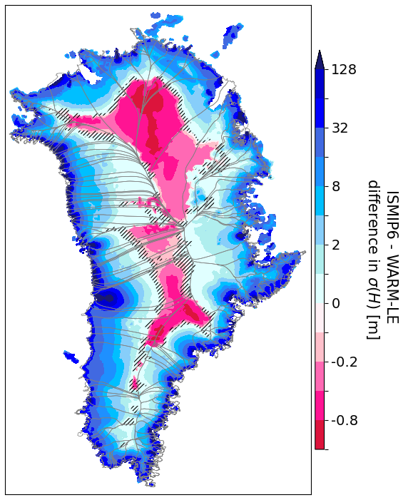
Figure 14 Difference between ice thickness spread (σ(H)) in 2100 for the ISMIP6 inter-model ensemble forced by MIROC5-RCP8.5 (Fig. 6b in Goelzer et al., 2020) and ice thickness spread in 2100 for WARM-LE. Blue indicates greater spread for ISMIP6 and pink for WARM-LE. Note the nonlinear and non-symmetric color bar. Hatching denotes non-significant differences, evaluated with a 300-sample bootstrap procedure for WARM-LE only and controlled for a false discovery rate of 0.05 (see Appendix H).

In the ISMIP6 protocol, all simulation results are presented as differences from a “control”, where SMB and ocean thermal forcing are held constant at 2014 values. In ISMIP6, ice sheet models demonstrate a diverse range of responses in this “control” simulation, with most models having less than 6 mm SLE mass gain or loss by 2100 and all ice sheet models simulating between 50 mm SLE mass gain and 15 mm SLE mass loss (with the 50 mm gain model being a strong outlier) (Goelzer et al., 2020). By comparison, in our study, CTRL-LE has ∼50 mm SLE mass loss by 2100. This difference is the result of our initialization procedure, which calibrates the model in order to reproduce the observed mass loss for the ice sheet between 2007 and 2017 (Fig. 2). While some ISMIP6 models do reproduce the historical mass loss trend for Greenland, this transient mass loss trend does not continue past the initialization of future simulations in 2014. This is likely due to most ISMIP6 models using a retreat parameterization whose boundaries would not move under fixed ocean thermal forcing, in contrast to the moving margins of our CTRL-LE.

Many ice sheet model projections included in ISMIP6 may be missing an important contributor to ongoing Greenland ice loss by not forcing a match to the initial transient of the GrIS. If the ice mass change in CTRL-LE is subtracted from WARM-LE, similarly to ISMIP6, the resulting anomalous mass loss in WARM-LE in 2100 is ∼70 mm SLE, which would fall just below the median of the range of model sensitivities in ISMIP6 (40–138 mm SLE). However, as we have explained above, this is strongly a function of our initialization scheme producing a strong transient ice loss even in the control setting, without mean climate change. Without subtracting control simulations, ice mass loss in WARM-LE would fall near the upper end of the range of ISMIP6 model sensitivities with ∼120 mm SLE. The IPCC handled this lack of capability by subtracting the control simulation from ISMIP6 simulations under future forcing and then adding the current ice sheet mass balance trend. This potential missing piece of simulated ice sheet mass loss in ISMIP6 has previously been identified by Aschwanden et al. (2021) and is the focus of efforts to improve ensemble design in the coming ISMIP7 effort.

Our initialization utilizes state-of-the-art methods (Choi et al., 2021) to match recent trends at both the ice sheet and the glacier scales. This procedure relies on the calibration of a stress threshold parameter in the von Mises calving law (Morlighem et al., 2016). However, since this is performed for each individual marine-terminating glacier, the number of degrees of freedom involved is as large as the number of glaciers, rendering our calibration prone to overfitting. Furthermore, given that marine glaciers have response timescales of the order of decades to millennia (Robel et al., 2018), matching 11-year observed trends is no guarantee of realistic model behavior. As discussed in Sect. 2.4, the 2007 ice sheet state is derived from a mass-conserving data assimilation scheme that integrates data that are not exactly co-located in time, producing inaccuracies which likely transiently adjust during the calibration window and potentially beyond 2018 into the ensemble simulations. Additionally, the exact timing of simulated rapid retreats at PG, ZI, and SK depends on the calibrated values of parameters used in the von Mises calving parameterization. We recognize that all calving parameterizations currently used in models have known issues when extrapolated across space and time (Amaral et al., 2020). We thus urge caution in interpreting the timing and extent of dramatic retreats of PG, ZI, and SK as realistic projections; instead, we suggest that these may reflect limitations of current tuning practices in ice sheet modeling. However, we emphasize that the aim of this study is not to project exact ice sheet evolution into the future but rather to quantify how uncertainty in ice sheet mass loss from climate variability is modulated by such rapid retreats and other processes.

4.3 Implications

One of the most significant results in this study is that when glaciers with significant potential for contribution to sea level rise undergo rapid retreats, uncertainty in total ice sheet mass loss increases rapidly. This rapid increase in uncertainty is predicted by theory (Robel et al., 2019) and has occurred in other parameter-perturbed ice sheet model experiments (DeConto et al., 2021; Lowry et al., 2021). However, because the retreats simulated for large glacier catchments in this study are short-lived, this elevated ensemble spread is equally short-lived when all ensemble members ultimately go through retreat. This is because the retreats simulated in this study are the combined result of increased flow and calving rates on short (<10 km) portions of bed topography that deepen towards the ice sheet interior. In Antarctica, many ice sheet models predict prolonged periods of rapid retreat over long overdeepenings (hundreds of kilometers; Seroussi et al., 2020, 2024). Thus, we can expect that a similar large-ensemble study conducted for Antarctica could produce long periods with strongly elevated ensemble spread. Prior idealized large-ensemble simulations of Thwaites Glacier, or representative configurations of it, show that its retreat under climate variability exhibits such an elevated ensemble spread over periods of decades to centuries (Robel et al., 2019; Hoffman et al., 2019; Bradley and Hewitt, 2024).

Our results indicate that the transient initial ice sheet tendency drives ensemble mean behavior for multiple decades before the mean climate forcing begins to play a more prominent role in controlling ice sheet behavior. This result highlights the critical role of initializing ice sheet models to match recently observed ice sheet behavior, which should ultimately reduce inter-model spread by providing a common point of comparison at least at the outset of simulations. The role of initialization can be hard to discern in multi-model ensembles such as ISMIP6 (Goelzer et al., 2020), where models adopt very different initialization procedures, or in parameter-perturbed ensembles, where parameter changes produce artificial disequilibria with the initial model state (DeConto et al., 2021). This will have the greatest influence on uncertainty in ice sheet evolution over timescales of decades, which are the most important for communities planning for sea level rise from ice sheet melt (Bassis, 2021). However, the absolute values of such uncertainties are ultimately just 1–2 mm sea level equivalent, which – like other sources of global sea level projection uncertainty – are relatively small compared to short-timescale uncertainties in coastal processes.

A final important finding of this study is that at the scale of the GrIS, SMB variability is the single largest component of climate variability contributing to ensemble spread. Under warming conditions, both increasing amplitude and spatial correlation of SMB variability also substantially contribute to ensemble spread. The non-stationarity in SMB variability has been observed in recent ice sheet mass balance (Boers and Rypdal, 2021) and surface mass balance (Slater et al., 2021) and is predicted by models to continue into the future (Fyke et al., 2014). It has been shown that such non-stationarity is expected as a result of increased poleward moisture transport (Bintanja et al., 2020).

An intercomparison of SMB models (Fettweis et al., 2020) shows that dEBM generally compares as well to 30 years of Greenland SMB observations as most other high-fidelity SMB models. Additionally, at the few locations of available high-resolution ice cores, Ultee et al. (2024) found that high-fidelity SMB models appear to represent the timescales of variability in a reasonable fashion. However, the lack of high-quality long-running SMB observations means that it is not possible to statistically validate the amplitude or timescales of variability simulated in dEBM across the entire ice sheet (and by extension AWI-ESM) in a robust fashion. Similarly, for TF, we rely on the timescales of variability simulated in AWI-ESM as there are almost no locations around Greenland with continuous records of ocean temperature at depth for several decades. The potential importance of time-varying SMB variability for uncertainty in ice sheet projections suggests that SMB models need to be calibrated, not just to match the mean, but also to capture the amplitude and spatial correlation of interannual variability and, critically, their multi-decadal changes. Using novel techniques for measuring SMB changes from ice cores at high temporal resolution (Trusel et al., 2018) will thus likely be critical to determining how SMB variability may change in warmer climates.

5 Conclusions

Internal climate variability has played an important role in mass change from the GrIS in the industrial era. In this study, we have shown that on decadal timescales, such aleatoric uncertainty will be an important contributor to projected ice sheet mass loss, regardless of anthropogenic emissions. These timescales are important for planning in coastal regions. Beyond a few decades, internal climate variability continues to drive increasing uncertainty in ice sheet simulations but at a level that is relatively limited compared to uncertainty from anthropogenic emissions and modeled ice sheet processes. During rapid glacier retreats, aleatoric uncertainty can grow rapidly, but in our simulations, these periods are short-lived, and the effect on ice loss uncertainty is localized to a few catchments in western and northern Greenland. Simulations of marine-terminating glaciers in Antarctica often produce more long-lived retreats due to differences in ice sheet geometry, thus raising the possibility of substantial and sustained aleatoric uncertainty in future ensemble projections of Antarctic ice loss.

While the representation of variability in climate models has improved substantially, in order to validate these models and calibrate stochastic parameterizations properly, high-quality observations are necessary. This study provides additional motivation for continuing and expanding such critical remote sensing and fieldwork efforts for the purpose of improving projections of future ice sheet change and the associated uncertainty.

Beyond quantifying the aleatoric uncertainty in simulations of future GrIS evolution, another central aim of this study is to provide a data set for the research community to aid in answering questions around the “natural” envelope of ice sheet and glacier variability in Greenland. The ensemble outputs are provided as open-access data sets, with information on access and data analysis detailed in the “Code and data availability” section. We hope that this resource will support continuing community efforts on the critical task of quantifying and reducing uncertainty in projections of future ice sheet change.

Appendix A: Calculation details

A1 Thermal forcing (TF)

We calculate TF with a salinity- and depth-dependent empirical equation for the freezing point (Cowton et al., 2015):

$$\begin{array}{}\text{(A1)}& \text{TF}(\mathbf{\text{x}},t)=T_{\text{oc}}(\mathbf{\text{x}},t)-\left({\mathit{\lambda }}_{\mathrm{1}}{S}_{\text{oc}}(\mathbf{\text{x}},t)+{\mathit{\lambda }}_{\mathrm{2}}+{\mathit{\lambda }}_{\mathrm{3}}z\right),\end{array}$$

where T_oc is the ocean temperature [°C]; S_oc is the ocean salinity [psu]; z is the vertical coordinate with respect to the surface level [m, positive upwards]; and λ₁,λ₂, and λ₃ are parameters set to $-\mathrm{5.73}\times {\mathrm{10}}^{-\mathrm{2}}$ °C psu⁻¹, $\mathrm{8.32}\times {\mathrm{10}}^{-\mathrm{2}}$ °C, and $-\mathrm{7.61}\times {\mathrm{10}}^{-\mathrm{4}}$ °C m⁻¹, respectively. The dependence on space and time is highlighted by x and t, respectively. Note that in Eq. (A1), TF is the depth-specific value, but in the main text, we use TF to indicate the depth-integrated value.

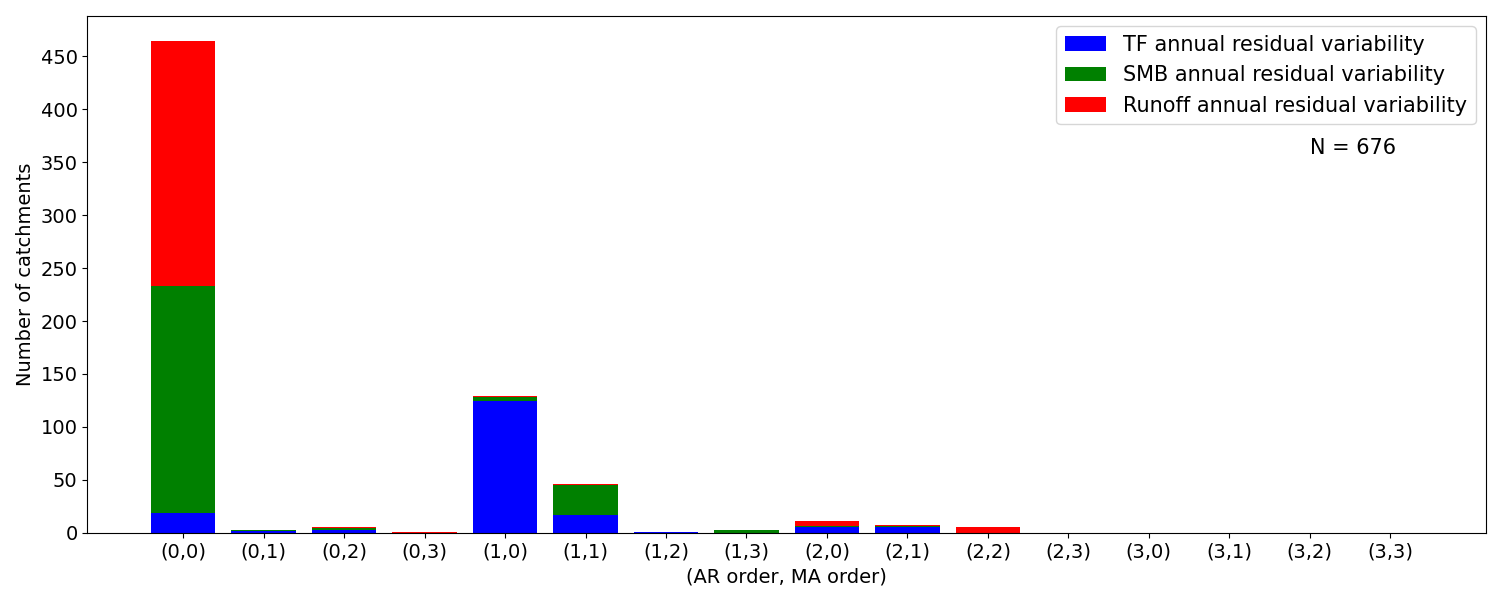
Figure A1 Histograms of best-fitting ARMA models for the 676 z-score time series. Results for the TF, SMB, and runoff time series are shown in different colors. Selection is based on the BIC. The autoregressive (AR) order and the moving-average (MA) order correspond to p and q in Eq. (A2), respectively. Results for AR and MA orders of 4 are not shown because they have histogram counts of zero.

A2 Autoregressive moving-average process (ARMA)

An ARMA process for a given variable y, of autoregressive order p and moving-average order q, is denoted as ARMA(p,q) and formulated as

$$\begin{array}{}\text{(A2)}& y_t=\sum _{i=\mathrm{1}}^p{\mathit{\phi }}_i{y}_{t-i}+\sum _{j=\mathrm{1}}^q{\mathit{\theta }}_j{\mathit{ϵ}}_{t-j}+{\mathit{ϵ}}_t,\end{array}$$

where the subscript t denotes the time step, and the AR and MA coefficients are denoted by φ₁, …, φ_p and θ₁, …, θ_q, respectively. The ϵ_t term is a Gaussian noise term. The φ_i coefficients capture the memory of the ARMA process, and the θ_i coefficients capture the persistence of random noise effects on the process evolution. We specify covariance between the different stochastic climate forcing variables through the Gaussian noise terms in the ARMA models. Specifically, a vector ϵ_t can be drawn from a multivariate Gaussian distribution of a dimension equal to the number of processes of interest:

$$\begin{array}{}\text{(A3)}& {\mathit{ϵ}}_t\sim N(\mathrm{0},\mathbf{\Sigma }),\end{array}$$

where Σ is the covariance matrix.

Figure A1 shows the selected ARMA combinations for the residual variability time series in TF, SMB, and runoff and for all the catchments. The Bayesian information criterion (Schwarz, 1978) is used for the selection procedure.

To generate stochastic annual time series of our three climatic variables (TF, SMB, and runoff), we use different covariance matrices (Σ in Eq. A3) for our different sub-periods separated by the 2000, 2050, and 2100 breakpoints. Given a correlation matrix C, a corresponding covariance matrix can be computed as

$$\begin{array}{}\text{(A4)}& {\mathbf{\Sigma }}_i={\mathbf{K}}_i{\mathbf{CK}}_i,\end{array}$$

where the subscript i stands for the ith sub-period, and K_i is a diagonal matrix with the marginal standard deviations of the ith sub-period on the diagonal. While the correlation matrix C used to compute the different Σ_i matrices remains identical, the amplitude of the variances changes through changing K_i. Therefore, we need to appropriately scale the marginal standard deviation of all ϵ_t terms (Eq. A2), denoted σ(ϵ). In particular, σ(ϵ) is not equal to the standard deviation of the y_t process (Eq. A2), denoted σ(y). Any σ(y) can simply be computed from a given time series, but the entries of K_i must be σ(ϵ). Thus, here we describe our method for estimating σ(ϵ) for all sub-periods of all 676 time series. For a given time series, we first calibrate the selected ARMA model (see Fig. A1) to the full time series. If both the p and the q orders (Eq. A2) are at most 1, there is an analytical expression to calculate σ(ϵ) (e.g., Wilks, 2011):

$$\begin{array}{}\text{(A5)}& \mathit{\sigma }\left(\mathit{ϵ}\right)=\mathit{\sigma }\left(y\right)\sqrt{{\displaystyle \frac{\mathrm{1}-{\mathit{\phi }}_{\mathrm{1}}^{\mathrm{2}}}{\mathrm{1}+{\mathit{\theta }}_{\mathrm{1}}^{\mathrm{2}}+\mathrm{2}{\mathit{\phi }}_{\mathrm{1}}{\mathit{\theta }}_{\mathrm{1}}}}},\end{array}$$

where φ₁=0 if p=0 and θ₁=0 if q=0. If p or q is greater than 1, we estimate σ(ϵ) numerically. We generate 10 time series from the calibrated ARMA process, starting with σ(ϵ)=σ(y). We iteratively decrease the estimate of σ(ϵ) until the mean total standard deviation of the 10 time series agrees with σ(y) within 0.1 %.

Appendix B: SMB–elevation profiles

Within-catchment spatial variability in SMB is captured through estimation of the slope of SMB–elevation profiles, referred to as lapse rates (e.g., Ultee et al., 2024). We compute lapse rates as the coefficients of a piecewise-linear regression of SMB versus elevation. We derive these functions using the dEBM SMB fields averaged over 2007 to 2203 because this corresponds to the period of our ice sheet simulations, as detailed in Sect. 2.3 and 2.4. We use two elevation breakpoints in our piecewise-linear functions, thus resulting in three separate lapse rates, which capture the typical pattern of strong SMB decrease with elevation in the ablation zone, smooth increase in the lower-accumulation zone, and gradual decrease at the uppermost elevations. In Fig. B1, we illustrate our fitting of lapse rate functions for four large GrIS catchments: Zachariae Isstrom, Helheim, Sermeq Kujalleq (Jakobshavn), and Humboldt. For catchments where the fitting procedure results in two breakpoints separated by less than 100 m of elevation, we use a single breakpoint. Similar to the lapse rate values, the elevation breakpoints are specific to each catchment.

Figure B1 Illustration of the SMB fitting as piecewise-linear functions of elevation. The dEBM mean 2007–2203 values are shown as black dots, and the fitted lapse rates are shown as the blue curves. The catchments shown are (a) Zachariae Isstrom in northeastern Greenland, (b) Helheim in southeastern Greenland, (c) Sermeq Kujalleq in central western Greenland, and (d) Humboldt in northeastern Greenland.

Appendix C: TF calculation caveat

In this study, TF is depth integrated from the surface (z=0 m) to the effective depth corresponding to the fjord sill (z_sill<0 m) following $\text{TF}=\left|z_{\mathrm{sill}}{|}^{-\mathrm{1}}{\int }_{z_{\mathrm{sill}}}^{\mathrm{0}}\text{TF}\right(z)\mathrm{d}z$, where TF is the depth-integrated value, while TF(z) is the depth-specific value. Our initial objective was to follow the procedure of Slater et al. (2020). However, Slater et al. (2020) not only integrate until z_sill, but also set the water properties below z_sill down to the glacier front depth (z_front<z_sill) to the water properties at z_sill. They then integrate TF over z_front by computing $\text{TF}=|z_{\mathrm{front}}{|}^{-\mathrm{1}}\left[{\int }_{z_{\mathrm{sill}}}^{\mathrm{0}}\text{TF}\left(z\right)\mathrm{d}z+\text{TF}\left(z_{\mathrm{sill}}\right)\left(z_{\mathrm{sill}}-z_{\mathrm{front}}\right)\right]$. We realized our error in not following the expression of Slater et al. (2020) only after the 372 simulations of this study had been performed, and we acknowledge this caveat in our results. However, we also believe that the impact of this caveat in the interpretation of our results is minor to minimal for the following reasons. (i) The assumption of within-fjord waters being linearly stratified and perfectly homogeneous below z_sill is subject to large uncertainties due to, for example, air–sea heat exchanges, within-fjord mixing processes, glacially modified water, and iceberg melting (e.g., Jackson and Straneo, 2016). The discrepancy between our TF calculation and the one from Slater et al. (2020) is likely much smaller than the uncertainty range of the true TF. (ii) Our computation of TF is consistent across all simulations, which implies that temporal variability and trends in TF are consistent with those simulated by AWI-ESM. (iii) Given that deeper waters on the Greenland shelf are typically warmer than surface waters, not integrating below z_sill likely slightly underestimates TF compared to the method of Slater et al. (2020). However, we calibrate (see Sect. 2.4.2) the calving sensitivity of all marine-terminating glaciers to their respective retreat rates over the observational record. As such, if there is any underestimation of the true TF at a given glacier, it is likely compensated for by an overestimation of calving propensity; note that frontal melting and calving at the terminus are treated identically by our ice sheet model.

Appendix D: Empirical sparse correlation matrix

Figure D1 shows the sparse correlation matrix between climate forcing variables and glacier catchments discussed in the Methods section.

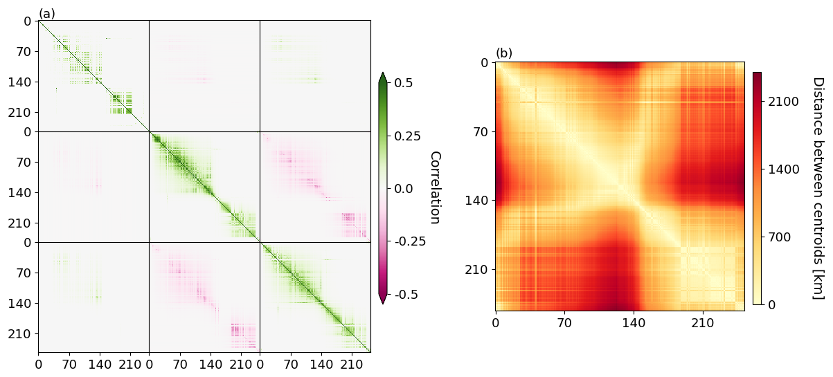
Figure D1 (a) Sparse correlation matrix of the residual variability in the three climatic variables (TF, SMB, runoff) for all 253 catchments. Each black square along the diagonal represents correlation over the 253 catchments for a variable, while each off-diagonal black square represents the cross-correlation over the 253 catchments for a pair of variables. The order of the climatic variables in the correlation matrix is TF (top and left), SMB (middle and middle), and runoff (low and right). The black lines separate submatrices specific to a pair of climatic variables for the 253 catchments. Catchment numbers correspond to a clockwise arrangement of the catchment centroids, starting from the northernmost catchment. Note that the color bar saturates at 0.5. (b) Distance matrix between the centroids of the 253 catchments. The discontinuity around catchment 140 corresponds to the shift between eastern and western Greenland.

Appendix E: Time evolution of standard deviation and skewness

Figure E1 shows the time evolution of the standard deviation and skewness for all large and small ensembles.

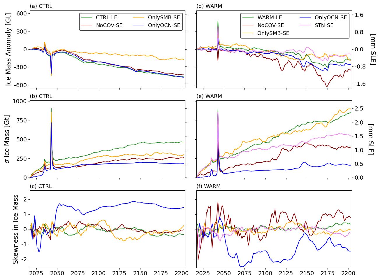
Figure E1 (a, d) Anomaly of the ensemble mean with respect to a corresponding deterministic simulation and (b, e) standard deviation and (c, f) skewness in the ice mass of the ensembles in the (a–c) CTRL climate forcing experiments and (d–f) WARM climate forcing experiments. Note that y axes are shared among panels of the same row. We recommend caution in interpreting the skewness of the small ensembles, which have only 30 members, because the skewness is a third-moment statistic and thus subject to large sampling uncertainty in small samples. See Sect. 2.5 for details about the large ensembles (LEs) and small ensembles (SEs). On the right y axes, mm SLE denotes millimeters of sea level rise equivalent.

Appendix F: Greenland-wide climate forcing

In this section, we illustrate the climate change forcing imposed under the RCP8.5 (WARM-LE) scenario compared to the pre-2000 (CTRL-LE) conditions. At the Greenland scale, the pre-2000 and post-2000 conditions can be compared in Fig. F1. The SMB time series is the annual Greenland-wide mean value, and the runoff time series is the annual Greenland total value. For the TF variable, we take the weighted mean of the individual marine-terminating glacier TF values, where weights are the area of the catchment drained by each glacier. SMB and runoff values are from the dEBM output, and TF values are from the bias-corrected and extrapolated values of AWI-ESM (see Sect. 2.2).

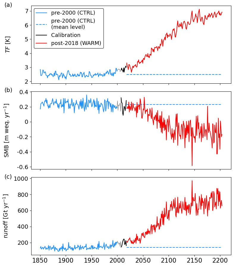
Figure F1 Greenland-wide values of (a) TF, (b) SMB, and (c) runoff. In (a), TF is the area-weighted average TF across all catchments with marine-terminating glaciers. In (b), SMB is the Greenland average. In (c), runoff is the Greenland total. The black section shows the calibration period (2007–2017). The red section shows the period on which statistics for the WARM-LE forcing are based. The blue section shows the period on which statistics for the CTRL-LE forcing are based. The grey sections are not used in any calibration procedures. The dashed blue lines show the mean conditions for CTRL-LE.

Appendix G: Ice thickness change during calibration period

Figure G1 shows a comparison of the total ice thickness change over the calibration period (2007–2017) in the model and in observations.

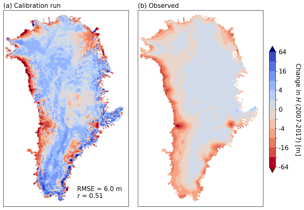
Figure G1 Total ice thickness change over the Greenland ice sheet during the model calibration period (2007–2017). (a) Modeled thickness change, smoothed with a 5 km Gaussian kernel. (b) Observed thickness change over the same period from Khan et al. (2025). Performance metrics provided are the root mean square error (RMSE) and the pattern correlation (r). Note the nonlinear color scale.

Appendix H: Statistical significance testing

When showing differences in ensemble mean or standard deviations between different ensembles, we test for statistical significance. We use a bootstrapping procedure with 300 bootstrap samples, each consisting of a random sampling with replacement of size equal to the original ensemble (100 for the large ensembles, 30 for the small ensembles). We compute the difference in the statistic of interest (mean and/or standard deviation) for each sample. We then compute the two-tailed p value for the event of zero difference.

For each Greenland map, there is one local statistical significance test per grid point. This situation is known as multiple-hypothesis testing. We report statistical significance by controlling for a false discovery rate (FDR) of 5 %. The FDR approach adjusts for test multiplicity by placing a strict limit on the fraction of significant grid cell results that are spurious (Wilks, 2016). In this procedure, we derive the critical p value for a test considered significant ($p_{\mathrm{FDR}}^{*}$) following

$$\begin{array}{}\text{(H1)}& p_{\mathrm{FDR}}^{*}=\underset{i=\mathrm{1}\mathrm{\dots }N}{\text{max}}\left(p_i:p_i\le {\displaystyle \frac{\mathrm{1}}{N}}{\mathit{\alpha }}_{\mathrm{FDR}}\right),\end{array}$$

where N is the number of local hypothesis tests, α_FDR is the FDR level chosen (5 % here), and p_i are the local test p values sorted in ascending order ($p_{\mathrm{1}}<p_{\mathrm{2}}<\mathrm{\dots }<p_N$). This method ensures that the selected FDR level is the upper limit for the overall expected proportion of erroneously rejected local null hypotheses among the rejections. This expectation holds regardless of the unknown proportion of local tests having true null hypotheses. In contrast, reporting significance on a local test on a local test basis only controls the probability of each individual true null hypothesis being erroneously rejected. As such, there is no overall control, and the proportion of erroneously rejected null hypotheses is an unknown function of the proportion of null hypotheses that should be rejected. Since the rejected hypothesis tests are of interest, i.e., non-zero difference, it is preferable to control the proportion of rejections that are meaningful. We refer to Wilks (2016) for details and examples.