The demise of the world's largest piedmont glacier: a probabilistic forecast

Sít' Tlein, located in the St. Elias Range, which straddles Alaska's Wrangell–St. Elias National Park and Kluane National Park in the Yukon, is the world's largest piedmont glacier. Sít' Tlein has thinned considerably over 30 years of altimetry, yet its low-elevation piedmont lobe has remained intact in contrast to the glaciers that once filled neighboring Icy and Disenchantment bays. In an effort to forecast changes to Sít' Tlein over decadal to centennial timescales, we take a data-constrained dynamical modeling approach in which we infer the parameters of a higher-order model of ice flow – the bed elevation, basal traction, and surface mass balance – with a diverse but spatiotemporally sparse set of observations including satellite-derived, time-varying velocity fields; radar-derived bed and surface elevation measurements; and in situ and remotely sensed observations of accumulation and ablation. Nonetheless, such data do not uniquely constrain model behavior, so we adopt an approximate Bayesian approach based on the Laplace approximation and facilitated by low-rank parametric representations to quantify uncertainty in the bed, traction, and mass balance fields alongside the induced uncertainty in model-based predictions of glacier change. We find that Sít' Tlein is considerably out of balance with contemporary (and presumably future) climate, and we expect its piedmont lobe to largely disappear over the coming centuries. If warming ceases, and surface mass balance remains at 2023 levels, then by 2073 (2173) we forecast a mass loss (expressed in terms of 95 % credible interval) of 323–444 km³ (546–728 km³). If instead surface mass balance continues to change at the same rate as inferred over the historical period, then we forecast a 2073 (2173) mass loss of 383–505 km³ (740–900 km³). In either case, the resulting retreat and subsequent replacement of glacier ice with a marine embayment or lake will yield a significant modification to the regional landscape and ecosystem.

1 Introduction

Sít' Tlein (briefly known as Malaspina Glacier; Fig. 1a), situated in coastal Alaska in the St. Elias Mountains, is the world's largest piedmont glacier and, when taken together with its neighbor the Bering–Bagley ice field, is Earth's largest temperate ice mass. Its geometry is complex and is comprised of a large piedmont lobe that is fed by three principal tributaries. The largest of these tributaries (sometimes independently referred to as Seward Glacier) has in its accumulation area Mt. Logan and Mt. St. Elias, the second- and fourth-highest points in North America, while its smaller tributaries, the Agassiz and Marvine glaciers, transport ice from the maritime windward slopes of Mt. St. Elias and Mt. Cook to within a few kilometers of the Gulf of Alaska. The total area of Sít' Tlein and its tributaries is roughly 4500 km², and the piedmont lobe has an estimated volume of nearly 700 km³ (Tober et al., 2023). The lobe's volume is constrained by radar observations of the ice geometry (Tober et al., 2023), but the volumes of the tributaries are not well known.

Sít' Tlein is thinning, and the glacier extent has diminished since it was first reliably mapped in the late 19th and early 20th century (Russell, 1893; Tarr and Martin, 1914; Sharp, 1958), with the active ice front, which previously extended to the ocean in some locations, now typically more than a kilometer removed. The combined system exhibits complex dynamics, with both the tributaries and piedmont lobe undergoing periodic surges that transport ice to regions that are otherwise stagnant and as such are critical for maintaining the piedmont lobe's geometry. These surges are spatially variable, with alternating directionality leading to dramatic looped moraines (Muskett et al., 2008). Notably, the lobe was at one point contiguous with piedmont glaciers that filled the adjacent Icy and Disenchantment bays (Barclay et al., 2001). This is reflected in the Tlingit name Sít' Tlein, which translates to “Big Glacier” and is also used to describe the extant Hubbard Glacier (Thornton, 2012), with its tidewater terminus located at the head of Disenchantment Bay. The conspicuous difference in retreat history between Sít' Tlein and its neighbors leads to the principal objective of this paper, which is to predict its future evolution – and in particular the potential future disintegration of its piedmont lobe.

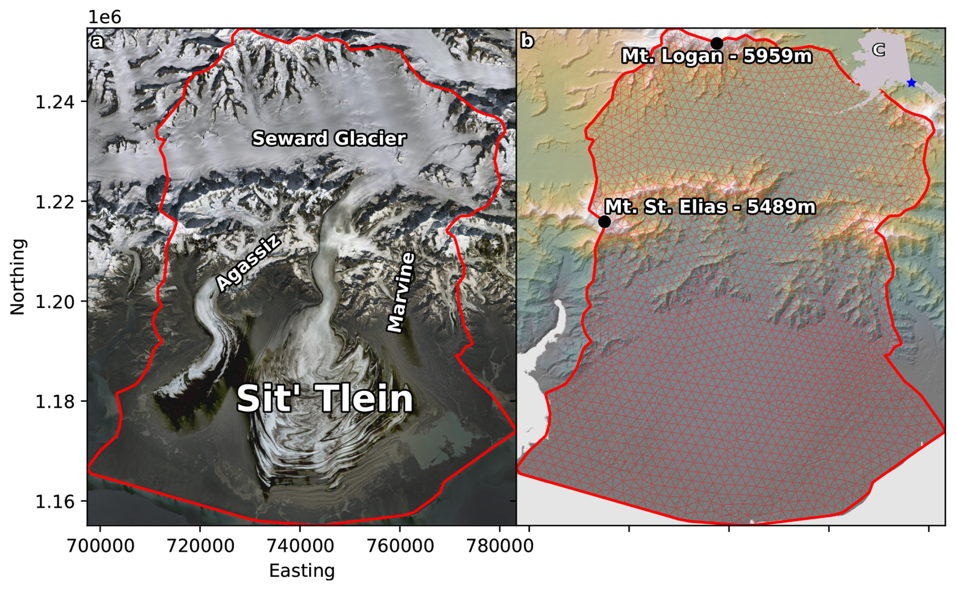
Figure 1 Sít' Tlein lobe and its tributary basins (a). A digital elevation model alongside our 1.5 km resolution finite-element mesh (b). The location of Sít' Tlein within the US state of Alaska (c, inset in upper right corner). The red outline indicates the model domain.

Our principal approach is through data-calibrated modeling. We use the ice dynamics model SpecEIS (Spectral Element Ice Simulator; Brinkerhoff, 2022; described in Sect. 2) – which we denote ℳ – to explicitly evolve the ice thickness H(x,t) and velocity field $\mathit{u}(\mathit{x},z,t)$ of Sít' Tlein from the year 1915 until 2344 based on past and assumed future climate forcings. While physics-based models are a useful tool for answering questions about glacier evolution under different assumptions of climate forcing, ice flow models in general and 𝖲𝗉𝖾𝖼𝖤𝖨𝖲 in particular are dependent on several critical inputs that govern the model's behavior. These inputs – so-called parameters – include the elevation of the glacier bed B(x), the spatiotemporally distributed frictional properties governing sliding at the glacier base β(x,t) (changes in which presumably control the observed surging at Sít' Tlein), the spatiotemporally distributed specific surface mass balance rate $\dot{a}(\mathit{x},t)$, and an initial ice thickness H₀(x) from which to begin the time evolution of the glacier geometry. Taken together, these form the vector

$$\begin{array}{}\text{(1)}& \mathit{m}=\left[H_{\mathrm{0}}\right(\mathit{x}),B(\mathit{x}),\mathit{\beta }(\mathit{x},t),\dot{a}(\mathit{x},t\left)\right].\end{array}$$

Each of these parameters exerts a leading-order control on glacier evolution. At Sít' Tlein (and elsewhere), we do not have a full characterization of m over space and time, which is an impediment to reliable projections of glacier change; however, some of its elements are partially observed at discrete locations and times. In this case we have spatiotemporally sparse radar-derived observations of the bed elevation $\widehat{B}$ and surface mass balance $\widehat{a}$. Such parameters also indirectly influence remotely sensed observations of surface velocity $\widehat{u}$ and aerial laser altimetry of surface elevation $\widehat{S}$. These data together form the vector of observations

$$\begin{array}{}\text{(2)}& \mathit{d}=[\widehat{S},{\widehat{\mathit{u}}}_s,\widehat{B},\widehat{a}].\end{array}$$

We seek to use these observations to constrain – to the extent possible – the model's parameters such that when used in conjunction with the ice flow model to predict glacier evolution over the period for which observations exist, predictions are consistent with observations. We do not use these observations to directly modify the evolving ice sheet geometry (as might be done in a reanalysis), so all such predictions are derived from a free-running model in a physically self-consistent way, similar in spirit to the oceanic inference engine ECCO (Forget et al., 2015). In practice, because the model parameters are continuous functions in space and time, we must make assumptions about how to represent them so as to be representable on a computer and to exhibit feasible physical properties such as smoothness. The construction of these representations is the topic of Sect. 3.

Because our observations are both imperfect and sparse, it is not possible (nor desirable) to identify a single ideal model configuration, and as such we adopt a probabilistic approach to prediction. Given a quantity of interest – which we call Δ(t) and which could represent change in elevation at a point, total ice volume, changes in meltwater flux, or any other model-derived quantity – we seek to characterize the probability distribution

$$\begin{array}{}\text{(3)}& \begin{array}{rl}P\left(\mathrm{\Delta }\right(t\left)\right|\mathit{d},\mathbf{F},\mathcal{M})& =\int P\left(\mathrm{\Delta }\right(t\left)\right|\mathit{m},f,\mathcal{M})\\ & \times P\left(\mathit{m}\right|\mathit{d},\mathcal{M}\left)P\right(f\left|\mathcal{F}\right)\mathrm{d}\mathit{m}\mathrm{d}\mathit{f},\end{array}\end{array}$$

where $P(\cdot |\cdot )$ denotes a probability density function over the first argument, with the second argument representing given conditions. This distribution can be interpreted in the sense of an ensemble of simulations of future change; ensemble members are drawn from the distribution of exogenous climate forcings P(f|ℱ) that are plausible under a chosen future climate scenario ℱ alongside endogenous (but data-constrained) parameters drawn from $P\left(\mathit{m}\right|\mathit{d},\mathcal{M})$.

As is typical for probabilistic prediction, we characterize Eq. (3) – the predictive distribution – in two steps. In the first step, described in Sect. 4, we infer the distribution of model parameters at Sít' Tlein given observations; i.e., we solve an “inverse problem”. This corresponds to finding the distribution over m such that resulting hindcasts over the historic period from 1915–2023 agree with available observations. This distribution – which we call the posterior – can be expressed as

$$\begin{array}{}\text{(4)}& P\left(\mathit{m}\right|\mathit{d},\mathcal{M})\propto \underset{\text{likelihood}}{\underbrace{P\left(\mathit{d}\right|\mathit{m},\mathcal{M})}}\underset{\text{prior}}{\underbrace{P\left(\mathit{m}\right|\mathcal{M})}},\end{array}$$

where we have used Bayes' theorem to write the posterior distribution as proportional to the product of a likelihood term, which measures the degree to which predictions made given a particular set of model parameters agree with the observations in hand, and a priori, which measures how likely said parameters were before observational constraint. Because our parameters are high-dimensional and our flow model nonlinear, characterizing this distribution exactly is not possible. To partially circumvent this we describe a numerical approximation method based on a local quadratic expansion and randomized low-rank matrix decomposition.

In the second step, described in Sect. 5, we approximate Eq. (3) under a handful of assumptions about future climate and calving dynamics by drawing a finite collection of random samples over future forcings and model parameters from the posterior distribution (Eq. 4), and using 𝖲𝗉𝖾𝖼𝖤𝖨𝖲 to predict a range of plausible glacier changes from present to 2344, with a particular emphasis on assessing the stability of the piedmont lobe.

2 Ice dynamics model

The posterior distribution over parameters is conditioned on a choice of model ℳ. This conditioning specifies which model parameters need to be inferred and also specifies – through the physical processes that the model represents – the way that a particular choice of parameter value is translated into something that can be compared against observations via the likelihood model.

Here we model glacier dynamics using the ice flow model 𝖲𝗉𝖾𝖼𝖤𝖨𝖲 (Brinkerhoff, 2023), which solves the coupled equations of mass conservation and stress balance defined over a domain Ω with boundary Γ. Mass conservation is expressed through the continuity equation

$$\begin{array}{}\text{(5)}& {\displaystyle \frac{\partial H}{\partial t}}+{\mathrm{\nabla }}_{\mathit{x}}\cdot \stackrel{\mathrm{‾}}{\mathit{u}}H=\dot{a},H>\mathrm{0}\text{on }\mathrm{\Omega }\text{(6)}& {\displaystyle }\left(\stackrel{\mathrm{‾}}{\mathit{u}}H\right)\cdot {\mathit{n}}_{\mathit{x}}=q_{\mathrm{in}},\text{on }{\mathrm{\Gamma }}_{\mathrm{in}},\end{array}$$

where $\mathit{u}(\mathit{x},z,t)$ is the ice velocity, $\stackrel{\mathrm{‾}}{\mathit{u}}(\mathit{x},t)$ is its vertical average, H(x,t) is the ice thickness, and q_in is a boundary flux (which we henceforth take to be zero). The stress balance (here the Blatter–Pattyn approximation (BPA) to the Stokes equations; Pattyn, 2003) is

$$\begin{array}{}\text{(7)}& {\mathrm{\nabla }}_{\mathit{x},z}\cdot \mathrm{2}\mathit{\eta }{\dot{\mathit{ϵ}}}_{\mathrm{1}}={\mathit{\rho }}_{i}g{\mathrm{\nabla }}_{\mathit{x}}S,\text{on }\mathrm{\Omega },\end{array}$$

where ρ_i and g are ice density and gravitational acceleration, $S(\mathit{x},t)=z_B(\mathit{x},t)+H(\mathit{x},t)$ the surface elevation, and ${\mathrm{\nabla }}_{\mathit{x},z}\equiv {\left[\frac{\partial }{\partial x_{\mathrm{1}}},\frac{\partial }{\partial x_{\mathrm{2}}},\frac{\partial }{\partial z}\right]}^T$. The elevation of the ice base is

$$\begin{array}{}\text{(8)}& z_B(\mathit{x},t)=max\left(z_{\mathrm{sl}}-{\displaystyle \frac{{\mathit{\rho }}_i}{{\mathit{\rho }}_w}}H(\mathit{x},t),B\left(\mathit{x}\right)\right),\end{array}$$

with z_sl the sea level. As such, Eq. (7) applies to both grounded and floating ice. ${\dot{\mathit{ϵ}}}_{\mathrm{1}}$ is the strain rate tensor subject to the simplifications of the BPA:

$$\begin{array}{}\text{(9)}& {\dot{\mathit{ϵ}}}_{\mathrm{1}}=\left[\begin{array}{ccc}\left(\mathrm{2}\frac{\partial u_{\mathrm{1}}}{\partial x_{\mathrm{1}}}+\frac{\partial u_{\mathrm{2}}}{\partial x_{\mathrm{2}}}\right)& \frac{\mathrm{1}}{\mathrm{2}}\left(\frac{\partial u_{\mathrm{1}}}{\partial x_{\mathrm{2}}}+\frac{\partial u_{\mathrm{2}}}{\partial x_{\mathrm{1}}}\right)& \frac{\mathrm{1}}{\mathrm{2}}\frac{\partial u_{\mathrm{1}}}{\partial z}\\ \frac{\mathrm{1}}{\mathrm{2}}\left(\frac{\partial u_{\mathrm{1}}}{\partial x_{\mathrm{2}}}+\frac{\partial u_{\mathrm{2}}}{\partial x_{\mathrm{1}}}\right)& \left(\frac{\partial u_{\mathrm{1}}}{\partial x_{\mathrm{1}}}+\mathrm{2}\frac{\partial u_{\mathrm{2}}}{\partial x_{\mathrm{2}}}\right)& \frac{\mathrm{1}}{\mathrm{2}}\frac{\partial u_{\mathrm{2}}}{\partial z}\end{array}\right].\end{array}$$

The viscosity – which depends inversely on the effective rate of strain and thus describes a shear-thinning fluid – is given by Glen's flow law

$$\begin{array}{}\text{(10)}& \mathit{\eta }={\displaystyle \frac{\mathrm{1}}{\mathrm{2}}}{A}^{-\frac{\mathrm{1}}{n}}{\left({\dot{\mathit{ϵ}}}_{II}^{\mathrm{2}}\right)}^{\frac{\mathrm{1}-n}{\mathrm{2}n}},\end{array}$$

with A the ice hardness, n the flow exponent, and ${\dot{\mathit{ϵ}}}_{II}$ the second invariant of the strain rate tensor. At subaerial lateral boundaries, we assume a stress-free condition, while at subaqueous boundaries we assume a normal stress given by water pressure. At the interface between ice and substrate, we assume a Budd-type sliding law (Budd et al., 1979)

$$\begin{array}{}\text{(11)}& \mathrm{2}\mathit{\eta }\dot{\mathit{ϵ}}\cdot \mathit{n}=-\exp \left(\mathit{\beta }\right)N\mathit{u},\end{array}$$

where N is the effective pressure, with water pressure assumed to be the maximum of 80 % of the ice overburden pressure or the sea level induced water pressure. This model of water pressure is motivated by the observation that water flows out of the terminus of Sít' Tlein at sea level, which places a lower limit on the water pressure beneath the glacier, alongside water pressure measurements from boreholes across many temperate glaciers, suggesting a high fraction of overburden as typical. Deviations from this mean-field approximation are subsumed into the specification of the traction coefficient β.

SpecEIS uses a mixed finite-element method for spatial discretization, representing ice thickness as cell-wise constants and velocity using specialized basis functions on mesh edges; a more detailed description of our approach can be found in Appendix A. Time discretization is fully implicit, using a backward Euler method solved with a damped Picard iteration. Model parameters like initial thickness, bed elevation, surface mass balance, and basal traction are represented internal to the model using a finite-element basis, but in the following sections, we work with those parameters using more expressive representations. We apply the model to Sít' Tlein using a 1.5 km resolution mesh, which is shown in Fig. 1b.

2.1 Integration with Pytorch

Because we seek to perform statistical inference and optimization using this model, we require the derivatives of (scalar functions of) the model outputs with respect to its inputs, i.e., the gradient of the average model error with respect to a parameter. At its simplest, an ice flow model can be written in a fully discrete form for a single time step (using the Markov property of the equations) as

$$\begin{array}{}\text{(12)}& [\mathsf{H},\stackrel{\mathrm{‾}}{\mathsf{U}},{\mathsf{U}}^{\prime }]=\mathsf{SpecEIS}({\mathsf{H}}_{\mathrm{0}},\mathsf{B},\mathit{\beta },\mathsf{a};\mathrm{\Delta }t),\end{array}$$

for some time step size Δt and in which upright symbols represent discretized variables (in this case finite-element coefficients). In this representation, inputs and outputs are both just arrays of numbers, and the resulting model becomes amenable to inclusion in a general purpose reverse-mode automatic differentiation (AD) framework such as Pytorch (Paszke et al., 2019). In the parlance of Pytorch, Eq. (12) constitutes a forward function. To implement a backward function we require a routine that efficiently computes the product of a vector with the Jacobian of the 𝖲𝗉𝖾𝖼𝖤𝖨𝖲 function. We use the adjoint method (e.g., MacAyeal, 1993, and Heimbach and Bugnion, 2009, in the glaciological literature) to evaluate such vector-Jacobian products (see Appendix B). This discrete and modular view is powerful because the thickness of the ice at the beginning of the time step is a function argument that will have a gradient associated with it when reverse-mode AD is applied. Reverse-mode AD generally and Pytorch specifically support arbitrary function composition; we can arbitrarily compose this discrete function with other functions. As we will see, these can be either complex routines for characterizing misfit, which will facilitate complex statistical treatment, or the function itself. The latter yields a fully time-dependent adjoint that can help determine the sensitivity of the model at the end of a simulation to parameter values at all times – for example the sensitivity of the average surface elevation error through time to a surface mass balance applied long in the past.

3 Representation of model parameters

The parameters in m to be inferred – the bed elevation B(x), the basal traction β(x,t), surface mass balance $\dot{a}(\mathit{x},t)$, and initial thickness H₀(x) – are each complex and continuous functions of space and (perhaps) time. As such, we introduce an approximating probabilistic model (i.e., a priori distribution) for each of these parameters, which we then make amenable to computer representation via decomposition into a finite set of basis functions. These representations are separate from the finite-element discretization, a distinction that is necessary because the characteristics of a finite-element mesh do not necessarily impose desired physical properties. However, we also introduce the necessary mechanisms for mapping samples from this basis to the finite-element mesh. In introducing these parameter models, we necessarily make some assumptions about smoothness and characteristic scales of variability while also making our representation independent of the numerical treatment of the model. This latter point is important because it allows for a natural hierarchy of mesh refinement in which some computational tasks can be performed with a coarsely defined ice flow model, whereas others can be performed with more detail. We emphasize that any explicit functional representation of model parameters is subject to potential misspecification (as is the flow model itself). However, doing so is also unavoidable, so we endeavor to be as transparent as possible about such assumptions. In addition to the specification of functional forms, it is also convenient to condition these priors (via Bayes' rule) when direct observations (i.e., observations that need not be used in conjunction with the ice flow model) are available. These data-constrained distributions, by virtue of our choice of prior family and data likelihood, are analytically tractable and are treated as an updated prior from the perspective of more complex inference involving 𝖲𝗉𝖾𝖼𝖤𝖨𝖲.

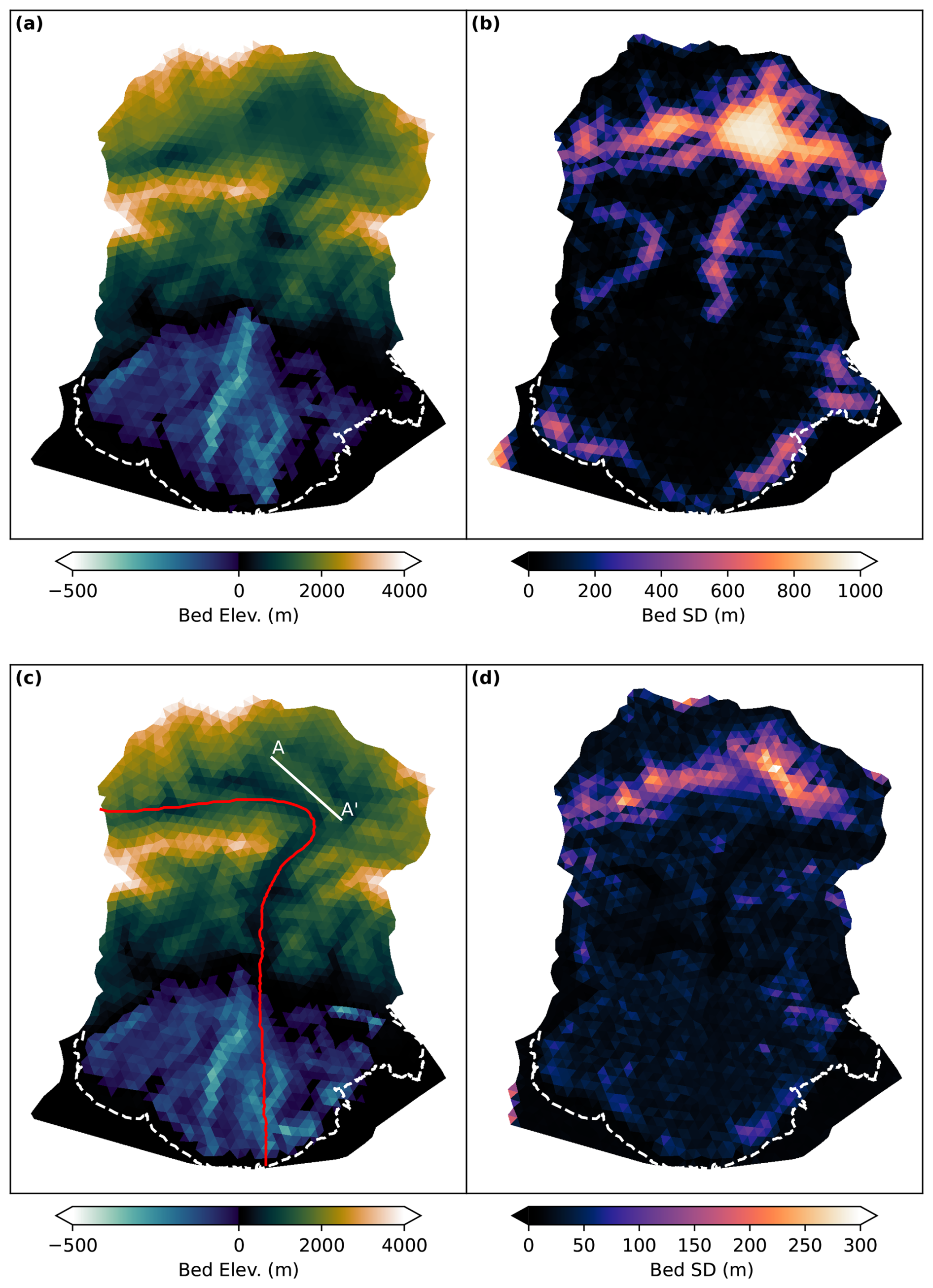
Figure 2 The prior mean (a), prior marginal standard deviation (b), posterior mean (c), and posterior marginal standard deviation (d) of the inferred bed elevation. The red line corresponds to the profile plotted in Fig. 4.

3.1 Bed

We represent the glacier bed elevation B(x) as a Gaussian process (GP) in space (Williams and Rasmussen, 2006), characterized by a mean function and a covariance function from the Matern family. Based on previous work (Tober et al., 2023), we set the characteristic length scale to 3 km and the amplitude to 1000 m. The mean function is modeled as a second-degree polynomial. To manage the computational complexity associated with GPs, especially for large spatial datasets, we employ a low-rank approximation of the covariance matrix. This reduces the parameter space while retaining the essential spatial correlation structure. This is done by expressing the bed elevation as a linear combination of a smaller set of basis functions, effectively reducing the number of parameters needed to be estimated. The specific approximation used here is based on structured kernel interpolation (Wilson and Nickisch, 2015), which decomposes the covariance matrix into a Kronecker product of smaller 1D covariance matrices, interpolated to the desired spatial locations. This approach avoids the need to explicitly construct and store the full covariance matrix. Further, by using the Nyström approximation for the decomposition of these smaller matrices we retain a desirable degree of sparsity in the resulting representation. This strategy allows for efficient computation of the GP, enabling us to represent the bed elevation with 4192 degrees of freedom, which are collected into a vector of basis coefficients with prior distribution $P\left({\mathit{z}}_B\right|\widehat{B})\sim \mathcal{N}(\mathrm{0},I)$, with z_B the basis function coefficients (which can be mapped to B(x) via a linear transformation). This distribution is conditioned on bed elevation observations from NASA's Operation IceBridge (Tober et al., 2023) and the Copernicus GLO-30 digital elevation model, resulting in a model that reflects both prior knowledge and observational data. Finally, we map this posterior distribution to the finite-element basis used in our ice flow model, ensuring consistency between the parameterization and the model's spatial discretization. The mean and marginal standard deviation of the resulting data-constrained distribution over B is shown in Fig. 2a and b. Further details of this procedure are described in Appendix C1.

3.2 Traction

Similar to the bed elevation, we model the basal traction field β(x,t) using a low-rank Gaussian process (GP), but extended to account for temporal variability. This results in a spatiotemporal GP with a separable covariance structure, where the spatial and temporal covariances are represented as a Kronecker product. We assume that the spatial covariance follows a Matern function with a characteristic length scale of 3 km, mirroring the bed elevation, while the temporal covariance follows a squared exponential function with a correlation scale of half a year. The spatial component of the GP is rendered computationally tractable using the same structured kernel interpolation approach employed for the bed elevation. The temporal component, being one-dimensional and relatively small, is computed directly via eigendecomposition. The resulting parameterization expresses the spatiotemporal basal traction field as a linear combination of spatial and temporal basis functions, substantially reducing the number of degrees of freedom. This representation facilitates efficient computation and allows us to readily map the field onto the CG1 finite-element basis used in the SpecEIS model. The resulting basal traction parameterization has 9443 degrees of freedom per year, which we collect into the coefficient vector z_β.

Figure 3 (a) Observations of surface mass balance from snow pits and cores and (b) data-constrained prior mean for surface mass balance, with the orange square representing the Mt. Logan snow core, green stars the core measurements described in (a), yellow triangles the ELA, and purple crosses observed melt measurements.

3.3 Surface mass balance

To parameterize the specific surface mass balance $\dot{a}(\mathit{x},t)$, we decompose it into two components: a spatially varying but time-invariant component and an elevation- and time-dependent component. The spatial component is modeled as a zero-mean Gaussian process with a squared exponential covariance function (characteristic length scale of 25 km and amplitude of 0.3 m a⁻¹). The elevation- and time-dependent component is modeled as a piecewise linear function of elevation, with specified values at key elevations, including sea level, the 2023 equilibrium line altitude (ELA), the median elevation of the accumulation zone, and the summit of Mount Logan. This component is further modulated by a linear trend in time and seasonal variability, represented by a scaled Vandermonde matrix and a temporal Gaussian process with a half-year timescale, respectively. We do not explicitly parameterize surface mass balance as a function of external climate forcing, instead opting to infer these relationships from observations in conjunction with other model parameters. This choice is motivated by the limitations and substantial disagreements among existing reanalysis products over our study region, particularly given the extreme topography of the St. Elias Mountains (Bieniek et al., 2016). The resulting model has 37 degrees of freedom, which are a priori distributed as $P\left({\mathit{z}}_{\dot{a}}\right|\widehat{a})=\mathcal{N}(\mathrm{0},I)$. This distribution is constrained with a diverse set of surface mass balance observations, including snow cores collected on Seward Glacier (Fig. 3a), aerial radar measurements of snow accumulation (Li et al., 2019), an inferred ELA from Landsat-8 imagery, and a high-elevation ice core from Mount Logan (Moore et al., 2002). We also incorporate a pseudo-observation representing a glaciological steady-state condition for the 2013 ice extent. These observations are combined using a least-squares approach, resulting in a posterior distribution over the surface mass balance field. The data-constrained prior mean for surface mass balance is visualized in Fig. 3b.

3.4 Initial thickness

The last parameter that we must define a distribution over is H₀(x), the initial thickness for the simulation (usually defined at some arbitrary time). It is challenging to develop a tractable representation in a similar manner to those described above because it is the only one that also corresponds to a physical quantity that is predicted by the flow model. It stands to reason that the initial simulation thickness ought to be one that is consistent with – or could have been generated by – the model itself. If this is not the case, then any prognostic model run beginning from this initial state must attribute some of its dynamical behavior to the shape of the ice surface changing to be consistent with the flow model's physics as well as the structural assumptions of the other parameters, as described in the previous three sections. Such an observation is not new and is the motivation for long (relative to the forecasting period) spin-ups of ice sheet models, in which a flow model is run to approximate steady-state, sometimes with modifications to bring this steady-state geometry into closer alignment with observations.

Here we use a data-constrained spin-up to eliminate the initial condition from consideration as a parameter. Specifically, instead of parameterizing the initial thickness through some basis representation, we take it to be given by the approximate steady-state solution produced by integrating the ice dynamics model over 2500 years with geometry as defined in Sect. 3.1, traction given by the time-averaged traction from Sect. 3.2, and the surface mass balance defined in Sect. 3.3 evaluated at some reference time that we take to be the start time for further time-dependent simulations. For this reference time, we take the year 1915, which is approximately when the maximum Little Ice Age ice extent occurred at Sít' Tlein based on geologic evidence, early cartography, and local knowledge (Tarr and Martin, 1914; Sharp, 1958). We note that we do have to specify an initial guess for this steady-state-finding routine (because we do not have numerical methods that can directly solve for the steady state without pseudo-time stepping, as in Bueler, 2016), and for this we use the 2013 surface elevation reported in the GLO-30 DEM. This initial condition does not, in principle, influence the final steady-state solution that we use as the initial condition for further simulations, so long as the steady-state solution is unique. This is the case for terrestrial glaciers (assuming a constant traction), where the mass balance uniquely specifies the ice extent. This may not be true for marine glaciers – for instance initializing Sít' Tlein from an ice-free state could preclude advance across the submarine basin to the present terminus position because of calving or flotation. However, because the 1915 and 2013 glaciers are both in extended configurations, our optimization procedure only explores the “extended” branch of this bifurcation, which effectively behaves as land-terminating.

4 Joint inference of model parameters

We now turn to the simultaneous inference of all parameters conditioned on all data. Written in terms of the finite basis function coefficients described above and using some conditional independence assumptions (namely that direct observations of one parameter do not affect any other parameters a priori), we write the joint posterior distribution over the combined coefficient vector $\mathit{\zeta }={\left[\begin{array}{ccc}{\mathit{z}}_B^T& {\mathit{z}}_{\mathit{\beta }}^T& {\mathit{z}}_{\dot{a}}^T\end{array}\right]}^T$ as

$$\begin{array}{}\text{(13)}& \begin{array}{rl}P(\mathit{\zeta }& |\widehat{S},\widehat{B},\widehat{a},\widehat{\mathit{u}})\\ & \propto P\left(\widehat{u}\right|\mathit{\zeta })\times P(\widehat{S}\left|\mathit{\zeta }\right)\\ \times & P\left({\mathit{z}}_B\right|\widehat{B}\left)P\right({\mathit{z}}_{\mathit{\beta }}\left)P\right({\mathit{z}}_{\dot{a}}\left|\widehat{a}\right).\end{array}\end{array}$$

The priors are as described above. In order to evaluate this function, likelihood functions remain to be specified for spatiotemporal observations of the surface elevation and velocity.

4.1 Surface elevation observations

We utilize two types of surface elevation observations. First, we use the publicly available Copernicus GLO-30 digital elevation model. This is the only product that offers complete coverage over Sít' Tlein and has a nominal date of 2013 with an estimated accuracy of 10 m. Second, we use elevations derived from airborne laser swath mapping, which were collected between 1995 and 2021 as part of either Operation IceBridge (Larsen et al., 2015) or an earlier campaign by Keith Echelmeyer (Arendt et al., 2002). These data were collected opportunistically and vary widely with respect to coverage, with earlier surveys characterizing only a predefined “centerline” and “cross-section”, whereas later surveys flew a denser grid-like pattern, especially over the piedmont lobe (see Fig. 6 for spatial coverage and elevation relative to the GLO-30 DEM for each observation year). These products have a nominal error of less than 2 m. For all elevation products we resample so as to have a density of approximately one observation per 500 m × 500 m, which we assume to be a safe minimum distance for assuming uncorrelated measurement error. The likelihood for surface observations is

$$\begin{array}{}\text{(14)}& P\left({\widehat{S}}_t\left|S\right(\mathit{x},t)\right)=\mathcal{N}\left(S(\mathit{x},t),{\mathbf{\Sigma }}_t^{\prime }\right),\end{array}$$

where S(x,t) is the evaluation of the model at observation points x at time t, and ${\mathbf{\Sigma }}_t^{\prime }$ is covariance matrix at time t encoding both observational errors and errors induced by model discretization. A derivation and precise definition of the covariance can be found in Appendix D.

4.2 Surface velocity

We also constrain model parameters via observations of surface velocity. For this project we use an adapted and standardized version of ITS_LIVEv1 (Gardner et al., 2018), a worldwide velocity product derived through a speckle-tracking cross-correlation method applied to LandSats 5, 6, 7, and 8. We use annual velocity mosaics, which have 120 m resolution and are available from 1985 until 2019. The nominal error in ITS_LIVE is variable, but on the order of 20 m a⁻¹. At Sít' Tlein, ITS_LIVE does not always have full coverage, particularly in the earlier years. As before, we downscale the observational density to one per 500 m × 500 m. We assume that each component of the velocity is normally distributed around the true (or predicted) value

$$\begin{array}{}\text{(15)}& P\left({\widehat{\mathit{u}}}_{it}\right|\mathit{u}({\mathit{x}}_i,t))=\mathcal{N}(\mathit{u}({\mathit{x}}_i,t),{\mathbf{\Sigma }}_u),\end{array}$$

where ${\widehat{\mathit{u}}}_{it}$ is the ITS_LIVE velocity vector observed at location x_i and time t, and u(x_i,t) is the modeled surface velocity at time t evaluated at the observation locations. We assume an observational standard deviation of 50 m a⁻¹; however, the error statistics of ITS_LIVE are not well understood, and this number is somewhat arbitrary.

4.3 Evaluation of the log-posterior

It is more convenient to work with the logarithm of the posterior distribution, for both numerical reasons (e.g., because it is less likely to over- or underflow) and symbolic ones (i.e., the chain rule of differentiation is easier to apply to a sum than a product). Because this function is monotonic, it induces no loss of information. We call this log-posterior function 𝒥(ζ)

$$\begin{array}{}\text{(16)}& \begin{array}{rl}\mathcal{J}\left(\mathit{\zeta }\right)& =\mathcal{L}\left(\mathit{\zeta }\right)+\mathcal{I}\left(\mathit{\zeta }\right)+C\\ \mathcal{L}\left(\mathit{\zeta }\right)& =\sum _{t\in {\mathcal{D}}_{\mathit{u}}}\log P\left({\widehat{u}}_t\right|\mathit{\zeta })\\ & +\sum _{t\in {\mathcal{D}}_S}\log P\left({\widehat{S}}_t\right|\mathit{\zeta })\\ \mathcal{I}\left(\mathit{\zeta }\right)& ={\mathit{\zeta }}^T\mathit{\zeta },\end{array}\end{array}$$

where ℒ is the log-likelihood with respect to the (yet-unused) observations of surface elevation and surface velocity, and ℐ is the log-prior distribution, which is exceptionally simple on account of our chosen reparameterizations, which renders all parameters uncorrelated and unit-normal. The summations in the above are taken over the years where observations exist for the given modality. We also note the presence of the constant C, which is a constant corresponding to the denominator in Bayes' rule that does not depend on the parameters.

While Eq. (16) describes our probability model in formal terms, it is also helpful to describe its evaluation narratively. Given values of z_B, z_β, and ${\mathit{z}}_{\dot{a}}$ (which initially have mean zero but which might be modified either through optimization or sampling), we map these to finite-element model parameters using our various constructed bases (and with the traction averaged over time and the mass balance evaluated ca. 1915. We then use 𝖲𝗉𝖾𝖼𝖤𝖨𝖲 to compute a steady state, which we take to be representative of the ice geometry in 1915. Using this geometry as an initial state, we run the model forward in time using a static bed elevation and time-varying traction and surface mass balance. Upon reaching the year 1985 (i.e., after 70 years of simulation time), observations of velocity and/or surface elevation become available, and while continuing to integrate the model forward in time until 2019, we also accumulate commensurate log-likelihood terms. At the end of the period of observations we also add the log-prior's contribution to the log-posterior.

The above computations are performed with Pytorch, which builds a computational graph of all operations, including the 𝖲𝗉𝖾𝖼𝖤𝖨𝖲 function described in Sect. 2. As such, after computing 𝒥, we can perform reverse-mode automatic differentiation on this graph, which computes the gradient of 𝒥 with respect to every intermediate computation in the graph. Importantly, this gradient computation also propagates through the pseudo-time stepping of the initial steady-state computation, which implies that the influence of the parameters on this initial condition – and its resulting teleconnection with the posterior log-probability – is accounted for.

Maximizing this function provides the most probable configuration of the bed, traction, and surface mass balance given all available observations, a so-called maximum a posteriori (or MAP) point. Performing this maximization is non-trivial, and we describe our approach in Appendix E.

4.4 Approximation of the posterior covariance

We seek to approximate the complete posterior given by Eq. (13), yet the procedure above yields only the most probable parameter values with respect to the posterior distribution. To quantify the posterior uncertainty, we employ the Laplace approximation, which approximates the posterior distribution as a multivariate normal with the MAP point as its mean. The covariance matrix is then determined through a second-order Taylor expansion of the log-posterior. Note that we do not characterize posterior uncertainty in the time-varying component of basal traction, which is very high-dimensional and requires prohibitive computation to characterize; however, we do characterize the posterior covariance over its mean.

Expanding the log-posterior around the MAP point, we have that

$$\begin{array}{}\text{(17)}& \begin{array}{rl}\mathcal{J}\left(\mathit{\zeta }\right)& \approx \mathcal{J}\left({\mathit{\zeta }}_{\mathrm{MAP}}\right)\\ & +{\displaystyle \frac{\partial J}{\partial \mathit{\zeta }}}\left(\mathit{\zeta }-{\mathit{\zeta }}_{\mathrm{MAP}}\right)\\ & +{\displaystyle \frac{\mathrm{1}}{\mathrm{2}}}{\left(\mathit{\zeta }-{\mathit{\zeta }}_{\mathrm{MAP}}\right)}^T\mathcal{H}\left(\mathit{\zeta }-{\mathit{\zeta }}_{\mathrm{MAP}}\right).\end{array}\end{array}$$

By the definition of the MAP point, the first-order term is zero, and we recognize this approximated log-posterior as a normal distribution with a covariance matrix given by the negative of the inverse of the Hessian 𝓗. Following Bui-Thanh et al. (2013) and Isaac et al. (2015), we decompose this Hessian into prior and likelihood parts

$$\begin{array}{}\text{(18)}& \mathcal{H}=({\mathcal{H}}_{\mathrm{data}}+I).\end{array}$$

The Hessian of the prior (which, once again, is unit-Gaussian and uncorrelated) is the identity matrix, while 𝓗_data is the Hessian of 𝓛 with respect to ζ. Direct computation of the data Hessian is intractable, both because it is very large and as such would be difficult to form – let alone invert – and also because it would require m function evaluations to compute. We instead approximate the inverse Hessian using a randomized matrix decomposition as described in Appendix F. This provides us with a matrix root to the approximate posterior covariance, which allows us both to inspect posterior uncertainty in parameters and to draw random samples from the distribution that we use to generate Monte Carlo forecasts in the next section.

5 Probabilistic forecasting

In the previous sections we develop a method for quantifying an approximate set of parameter values that produces model predictions that are consistent with observations, i.e., the posterior distribution over parameters corresponding to the second term inside the integrand in Eq. (3). We now turn to using these parameter values to make predictions about future change at Sít' Tlein. Our approach to this problem is simple and does not require a complex numerical treatment; we take the classic ensemble modeling approach of drawing as large a set of parameters as computationally feasible and run the model forward in time with those parameters. The resulting approximation to the predictive distribution is

$$\begin{array}{}\text{(19)}& \begin{array}{rl}P\left(\mathrm{\Delta }\right(t\left)\right|\mathit{d},\mathcal{F})& \approx {\displaystyle \frac{\mathrm{1}}{n_s}}\sum _{j=\mathrm{1}}^{n_s}P\left(\mathrm{\Delta }\right(t\left)\right|{\mathit{m}}_j,f_j)\\ {\mathit{m}}_j& \sim P\left(\mathit{m}\right|\mathit{d})\\ f_j& \sim P\left(f\right|F).\end{array}\end{array}$$

While such Monte Carlo methods converge slowly, they are easy to implement and are embarrassingly parallel.

We integrate the model from a steady state at 1915–2344. Each model has a different resulting geometry and pattern of flow, and from these we evaluate quantities of interest at different times. We qualitatively divide the predictive distribution into a hindcast (from 1915–2023) and forecast (from 2023 onward). The distribution over parameters for the hindcast is unambiguous, but forecasting requires some assumptions about future changes to time-evolving parameters.

• Steady geometry. We assume that the bed elevation remains constant (although we relax this assumption for an ancillary experiment).

• Periodic surges. We assume that the 36-year inferred record of time variation in the basal traction repeats in a periodic fashion. While we do not believe that this approach will necessarily predict the precise location, timing, and magnitude of future surges, we believe that it will capture their statistical features and their resulting influence on geometric change. As is evident from the repeating nature of Sít' Tlein's looped moraines (Muskett et al., 2008), we do not expect surge dynamics to depart qualitatively from the pattern observed before, at least in the short term, although this assumption is likely to become less valid if Sít' Tlein undergoes a major geometric change. Nonetheless, this choice is also governed by necessity, since we currently lack a validated and general mechanistic model for sliding generally and one that can predict surging specifically. To test whether this mechanism plays a substantial role in ice evolution, we also conduct an experiment in which we make projections with traction fixed to the inferred mean.

• Projected and frozen mass balance. We explore two scenarios for future evolution of the surface mass balance. Recalling that we parameterize the surface mass balance for different elevations as a linear function of time since 1915, in our first scenario we linearly extrapolate these trends into the future, which would be roughly commensurate with a linear extrapolation of mean air temperature over the last 4 decades. Based on the CMIP6 ensemble (Lee et al., 2021), this is in rough correspondence to the SSP3-7.0 scenario, which represents a high, but plausible, potential for warming until around 2100 and is somewhat higher than SSP5-8.5 at 2300. As a second scenario, we consider an end-member case in which we freeze the surface mass balance field at 2023 and hold it constant into the future, which corresponds to an immediate cessation of warming.

• Calving. One final consideration that we need to address is calving. While contemporary Sít' Tlein does not undergo much mass loss due to calving, it does have small calving fronts on the margins of two proglacial lakes, and at least one of those lakes is already receiving tidal inputs of marine saltwater (Thompson et al., 2021). We therefore expect that if the glacier undergoes additional retreat, it could develop a broad marine- or lake-terminating calving front, as is the case for its nearby neighbors in Disenchantment Bay, Icy Bay, and the Bering Glacier. Because we cannot yet observe calving here, we cannot infer the values of parameters governing a forward calving model. While marginalization over a calving velocity prior is possible, here we simply examine two end-member scenarios to bracket possible future behavior. In the first, we assume that calving does not occur; this is not to say that ice does not float – we do allow floating tongues to form. This is perhaps not unrealistic for lake-terminating glaciers, which in coastal Alaska have been observed to develop sizable floating tongues (Truffer and Motyka, 2016). In the second scenario, we adopt a calving-on-flotation criterion and associate with floating ice a calving velocity of 1 km a⁻¹, which roughly corresponds to the observed retreat rate at Columbia Glacier.

We perform ensemble experiments using combinations of each calving and climate evolution assumption stated above, for a total of four experiments. In each of these four experiments, we assume both steady geometry and periodic surging.

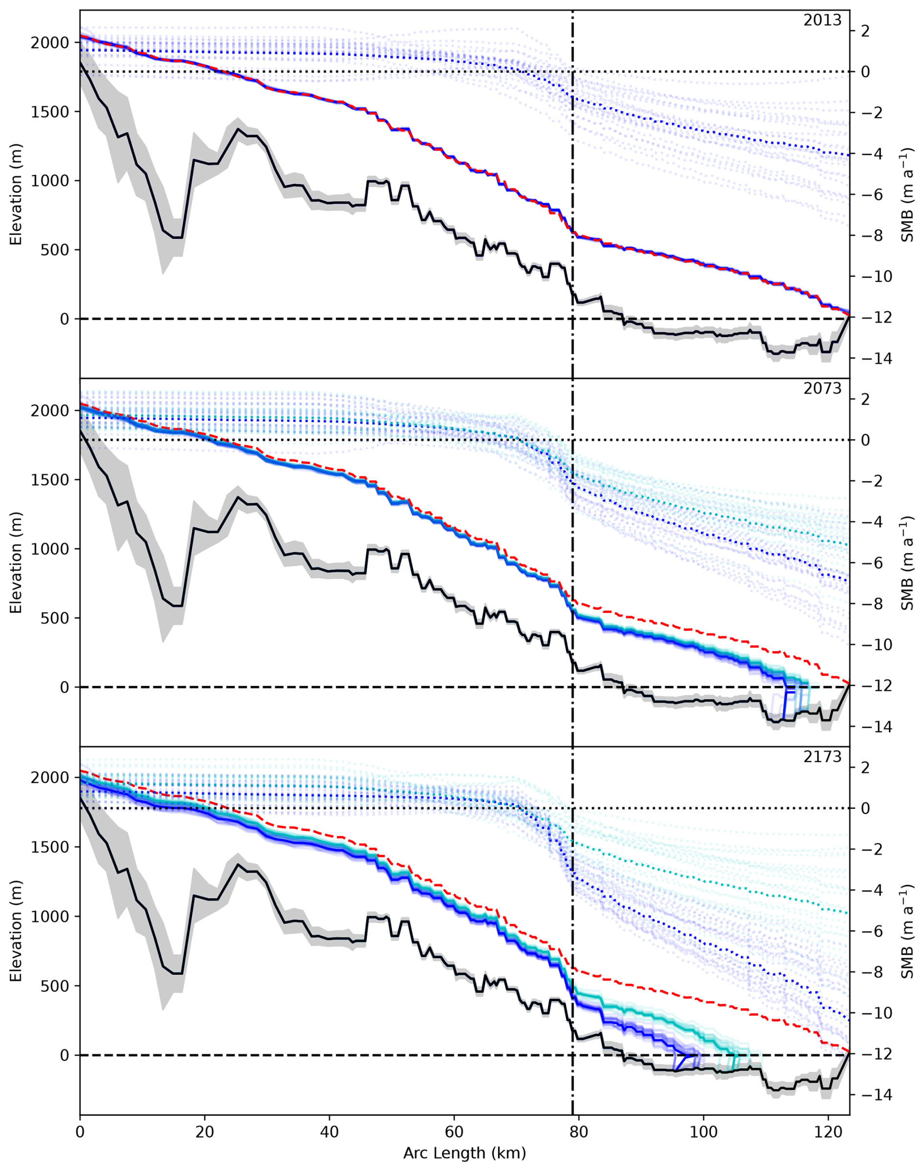
Figure 4 Profile of ice geometry corresponding to the red line in Fig. 2 at 2013, 2073, and 2173. Solid cyan and blue lines are surface elevations corresponding to individual ensemble members for climate assumptions in which surface mass balance is frozen at 2023 values or extrapolated into the future, respectively. Dotted cyan and blue lines are the corresponding surface mass balance curves. The dashed red line shows the 2013 ice surface for reference. The black line indicates the most probable bed elevation, with the gray envelope showing 2 standard deviations. The vertical dash-dotted line shows the approximate location at which the Sít' Tlein piedmont lobe begins.

6 Results

In this section we describe both the posterior distribution over data-informed model parameters alongside the predictive distributions over both the hindcast and forecast periods generated by sampling from the posterior and running the ice dynamics model from 1915 until 2344. An analysis of model performance against unseen data is given in Appendix G.

6.1 Bed geometry

We begin with an analysis of the inferred bed elevation. Figure 2c shows the most probable bed elevation. Much of this map reflects direct observations of the bed taken via radar sounding; however, features that were not imaged by radar, particularly in the accumulation area at the northern end of the map, are also captured. Most salient of these is the presence of a subglacial mountain range (Transect A-A' in Fig. 2c) that continues trending southeast from the flanks of Mt. Logan, which divides the principal accumulation area for the Seward Lobe into two separate regions. The surface expression of this feature as visible on a digital elevation model is subtle; however, on the ground this feature is conspicuous and associated with a large crevasse field and an increase in ice surface gradient. Interestingly, the uncertainty in bed elevation over this region (shown in Fig. 2d) is relatively low, indicating that the surface observations of velocity and especially surface elevation strongly constrain the bed in this region. In contrast, the basins to the northeast and southwest of this ridge, while fast-flowing, have relatively homogeneous topography and low gradients, which leads to greater uncertainty. Another region that exhibits high uncertainty in elevation are the areas very near the margin of Sít' Tlein's piedmont lobe. This uncertainty is the result of the lack of dynamics in this region; without significant flow, the observations of velocity (which are nearly zero) and geometry (which is uninformative in low-slope regions) provide little information, and the posterior variance is nearly the same as that of the prior. While there are few bed measurements within the fast-flowing trunk of Seward Glacier as it flows through the gap in the St. Elias range, the posterior uncertainty there is similar to that in regions constrained by direct bed observations, indicating that ice dynamics provides a strong constraint.

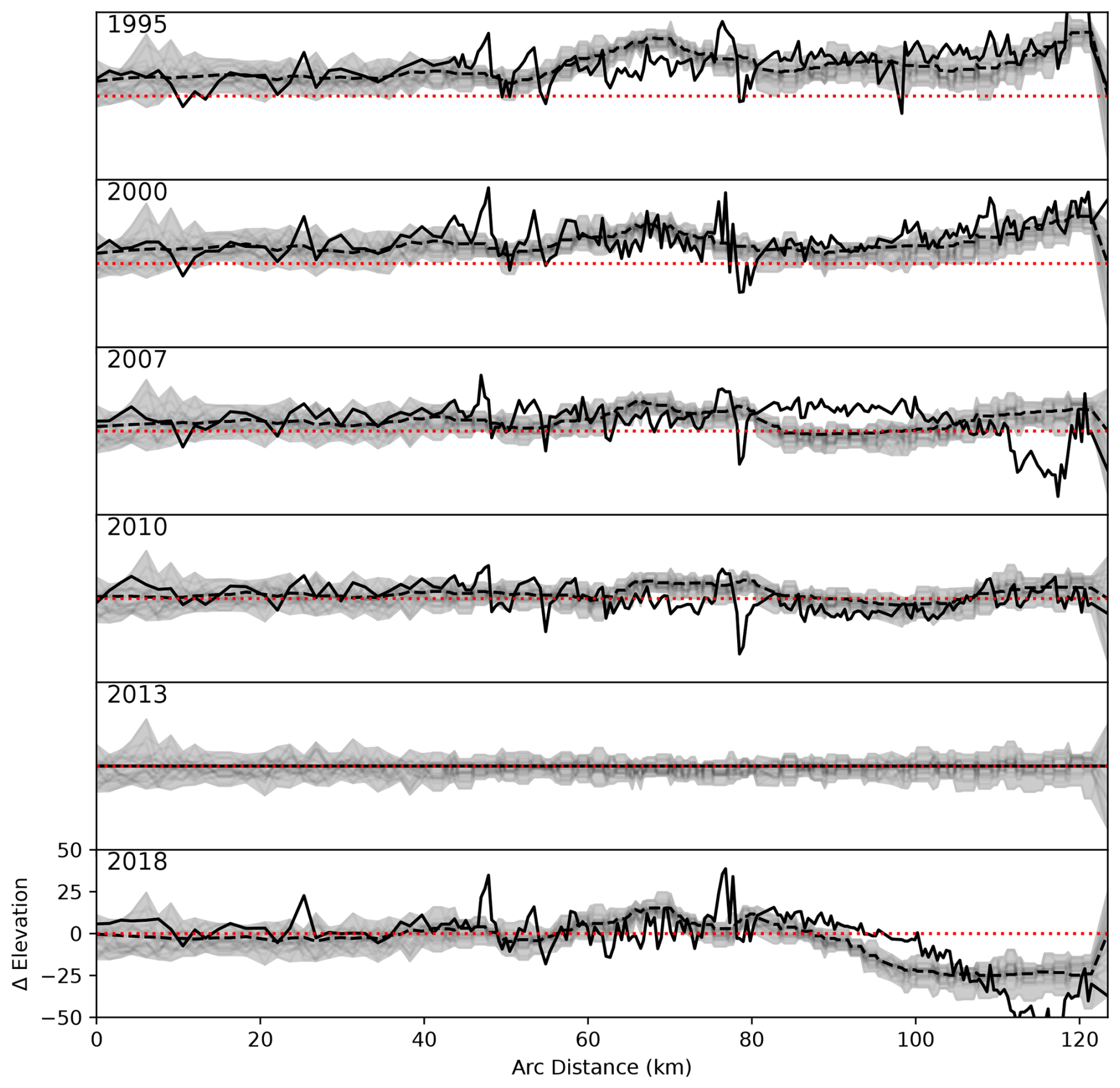
Figure 5 Observed (dashed) and MAP-predicted (solid) surface elevations relative to the 2013 COP30 DEM for a selection of years plotted along the red line shown in Fig. 2. Envelopes represent the range of elevations for these computed for 50 random samples from the posterior distribution.

It is also instructive to observe the geometry in cross-section. Figure 4a shows the inferred bed elevation along the red profile indicated in Fig. 2c. We also see here the pattern of relatively high bed uncertainty in the accumulation zone, with low uncertainty in areas with fast flow or direct measurements. This figure also shows the resulting surface geometry for 50 random samples drawn from the posterior distribution and integrated through time, evaluated at the year 2013. We see a strong agreement between random surface samples and the observed surface elevation, especially relative to the vertical scale of the system, in which all simulations are atop one another at this scale. The surface mass balance curves associated with each of these profiles show considerable variability, primarily due to annual noise that cannot be reduced by temporally limited observations and the influence of which has little direct influence on annual surface elevation or velocity changes. Nonetheless, we infer a mean contemporary surface mass balance at sea level, which was not part of the observational dataset, to be approximately 4 m a⁻¹.

6.2 Elevation change

Zooming in on the surface and plotting the modeled and observed surface elevations relative to 2013 for years in which observations exist (Fig. 5), we find that the predicted surface elevation matches observations in both absolute magnitude and in trend. However, there is still some spread in the distribution due to assumed uncertainties in the surface elevation observations. Figure 6 shows the spatial distribution of the model's most probable predicted elevation change relative to 2013 alongside sparse observations. We find good agreement between the broad spatial patterns, but the match is imperfect, particularly in later years over the piedmont lobe in which the data indicate a drawdown that is presumably the result of a surge that we have not adequately captured, alongside a perhaps too-simple surface mass balance parameterization. Of particular scientific interest, it is evident from observations that the ablation zone is thinning much more quickly than is the accumulation zone, and the spatiotemporal variability in the inferred surface mass balance – and the resulting modeled thinning – reflects this pattern as well. The misfit between the model and observations is shown in Fig. 7. We generally find that the MAP surface approximates observations to within 20 m over smooth, ice-covered regions.

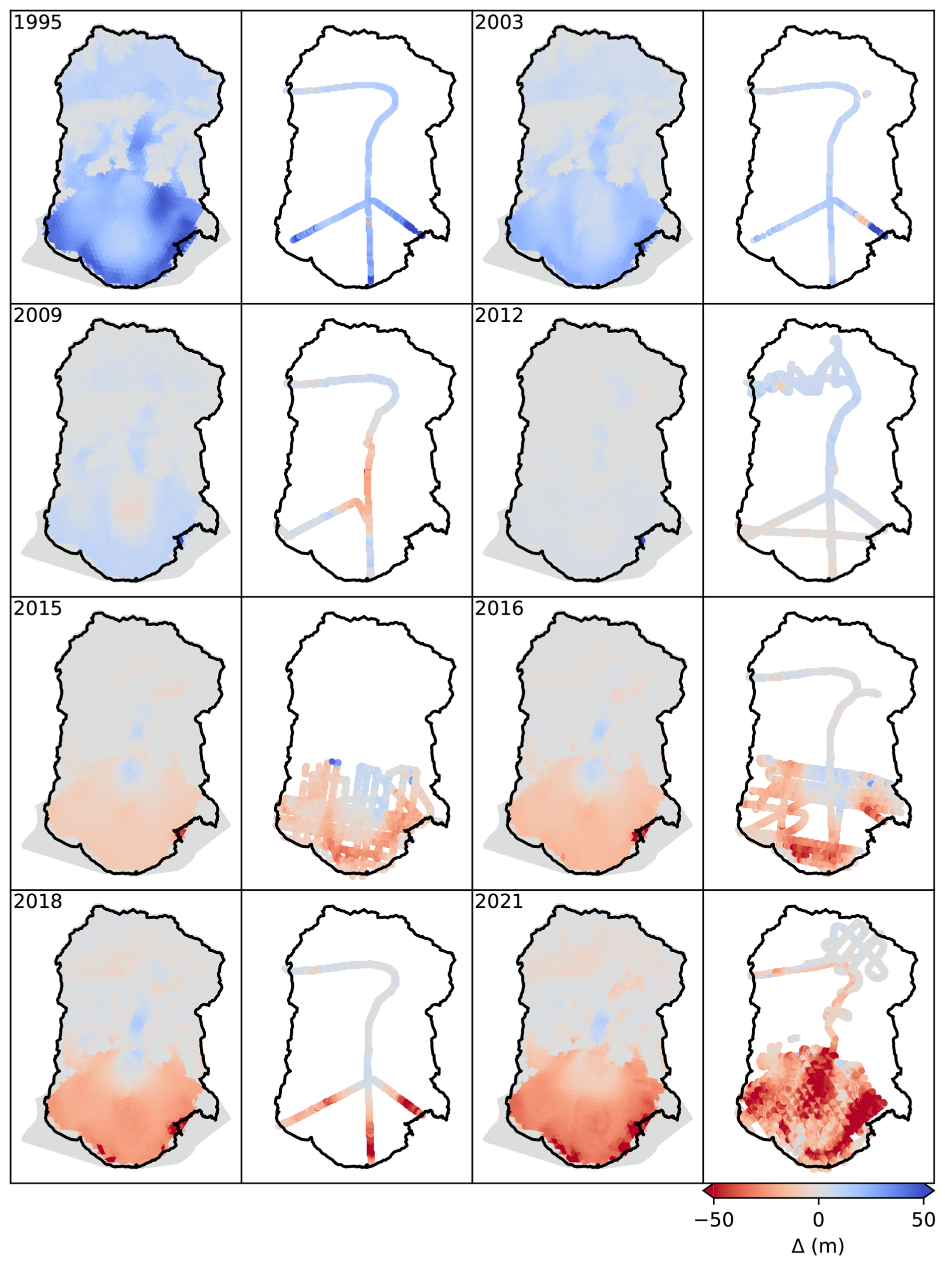
Figure 6 Modeled (left) and observed (right) surface elevations relative to 2013 for selected years.

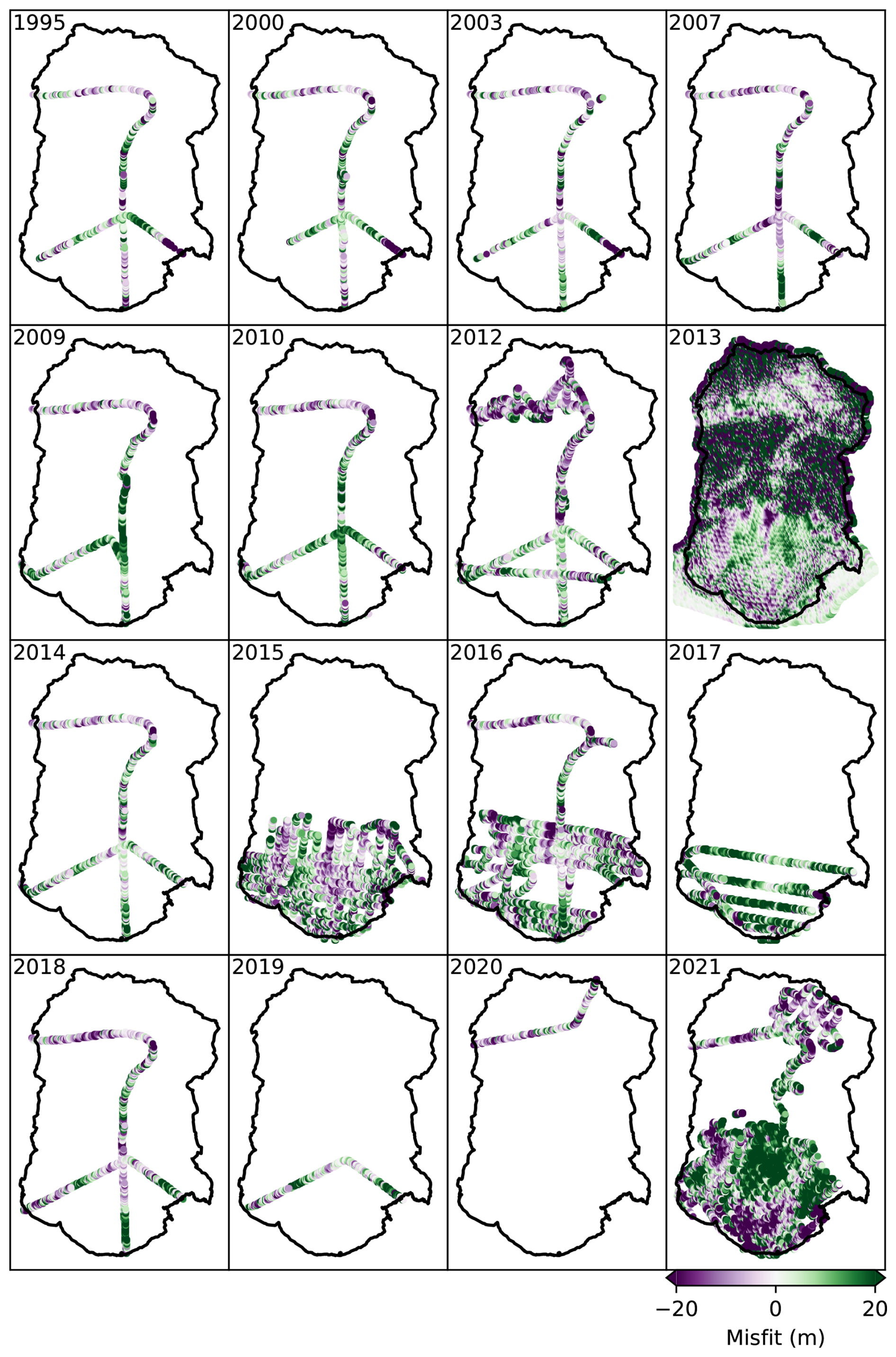
Figure 7 Predicted surface minus observed surface for all years for which data are available. The color scale saturates at 20 m.

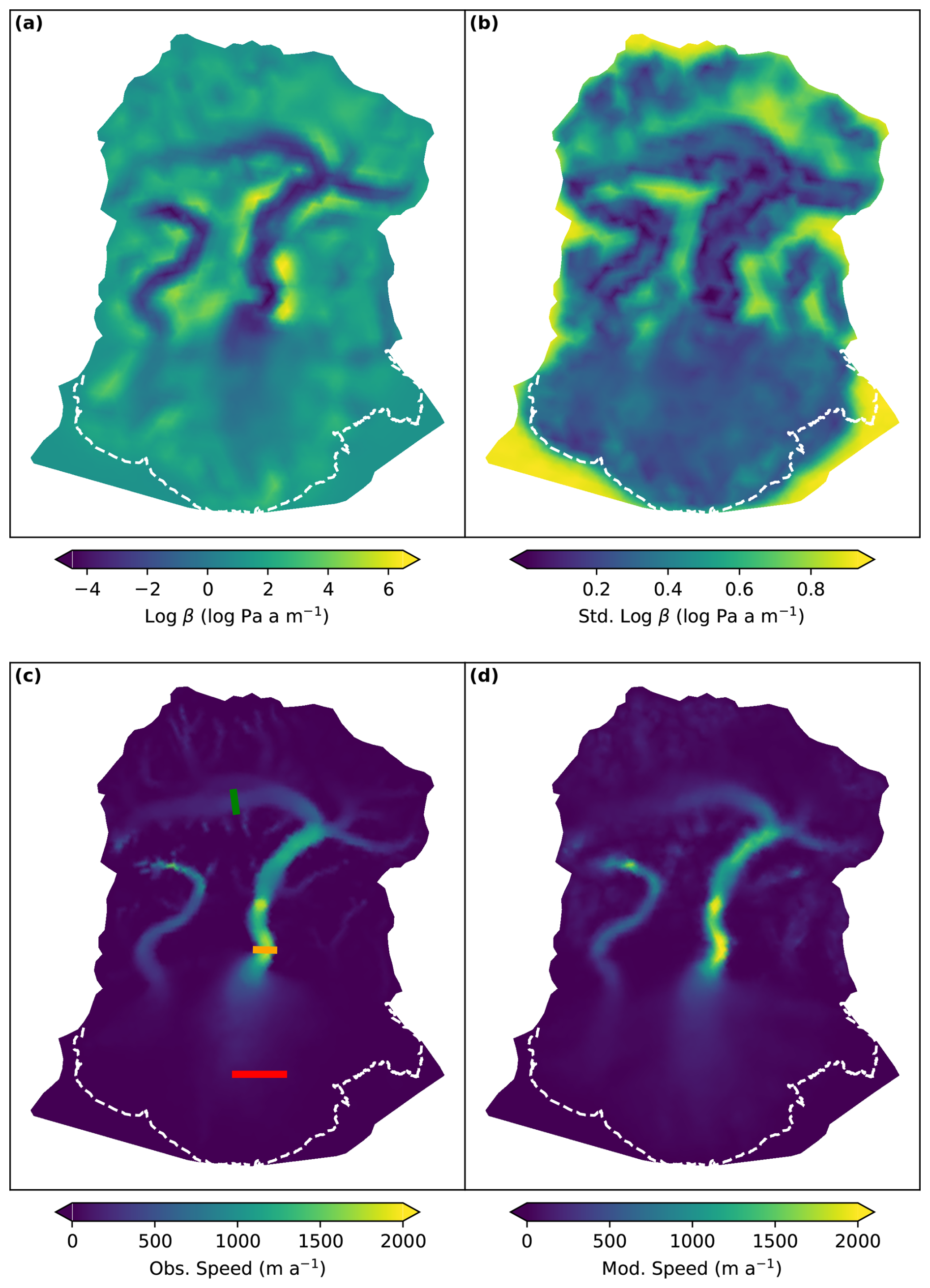
Figure 8 Mean (a) and standard deviation (b) of the basal traction field. Observed (c) and modeled (d) speed averaged over the years 1985–2019. Included in (c) are also transects over which velocity is averaged and displayed as a function of time in Fig. 9.

6.3 Traction and velocity

Figure 8a shows the inferred mean basal traction field. regions of fast flow exhibit low traction, with relatively low posterior variance (Fig. 8b) in regions well constrained by velocity observations. As is to be expected, steep or ice-free areas without velocity measurements exhibit a high posterior variance.

More interesting than the traction fields themselves – which mostly alias unknown physical processes – is the resulting velocity field, the temporal mean of which is shown in Fig. 8d alongside the mean observation. While this is an expected result since the inference of basal traction to match surface observations is well established, we find good congruence between the modeled and observed value over areas with fast-flowing ice. This fit is once again not perfect, particularly in steep regions (where the model predicts relatively fast flow that corresponds to what would likely be avalanche transport in the real world) and in slow regions of the lobe, where faster flow than is identified in the observations is necessary to maintain contemporary geometries. This latter effect could be attributed to two (not mutually exclusive) possibilities. First, the flow rates in the slow parts of the lobe may simply be below ITS_LIVE detection thresholds and so are spuriously assigned a zero velocity. Alternatively, it may be the case that some parts of the piedmont lobe are replenished by velocity configurations that do not exist in the 36-year observational record. Sít' Tlein is a surge-type glacier, so it is reasonable to imagine that some parts of the lobe were not recipients of upstream ice flux during this time period, yet the model must route ice to these areas to ensure that they are not modeled as ice-free. This in turn could be exacerbated by errors – particularly those induced by model inadequacy – in the modeled surface mass balance field.

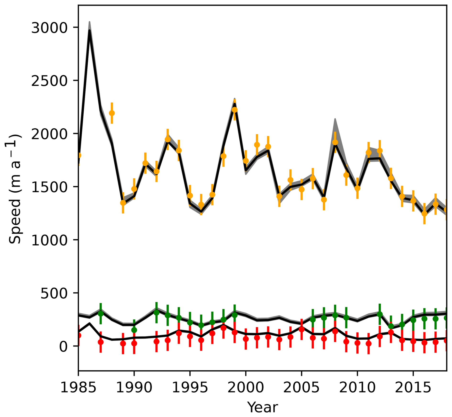
Figure 9 Time series of average speed computed over the equivalently colored cross-sections in Fig. 8c. Points indicate ITS_LIVE annual velocity mosaics with assumed 2σ errors, while the continuous lines are associated model evaluations.

While the primary long-term dynamics of Sít' Tlein are likely controlled by time-averaged velocity, we also explicitly model a time-varying traction so as to match the evident surges in the observational record. Fig. 9 shows the time series of velocity magnitude averaged over the three profiles shown in Fig. 8c. In Sít' Tlein's fast-flowing trunk, we recover the time series of velocity with high fidelity. Because the posterior uncertainty in traction is low there, and also because we do not capture the posterior variance over the time-varying component of the traction, the predicted variance in velocity is also low. The moderately fast-accumulation area exhibits similar properties. Again, we find that areas near the ice margin generally have flow speeds that are somewhat too fast, for reasons described previously. A complete spatially and temporally distributed comparison of predicted versus modeled velocity anomalies is shown in Figs. S1–5.

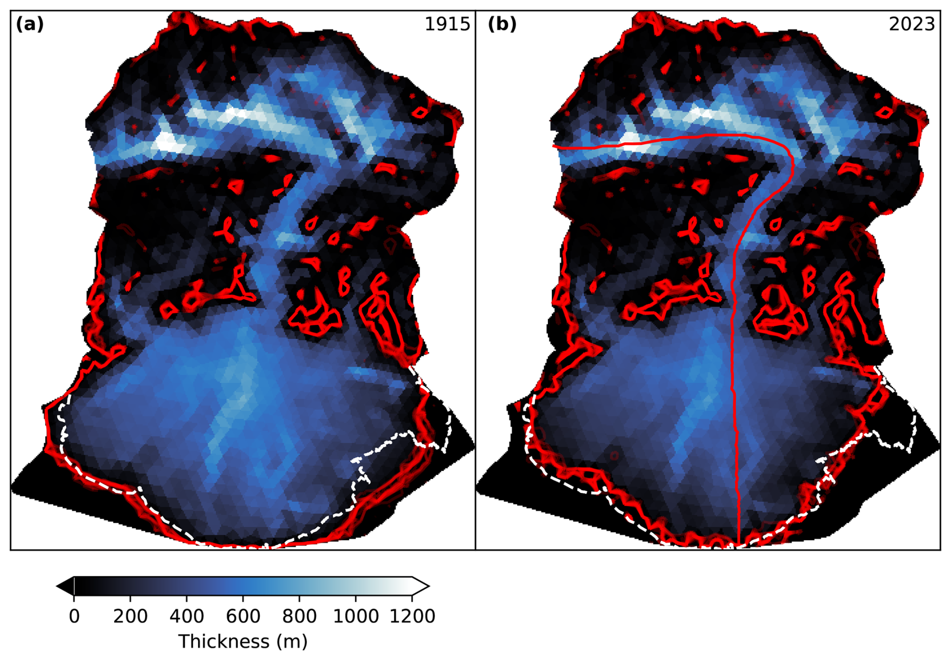
Figure 10 Predicted ice extent at the beginning and end of the hindcast period. Red lines indicate terminus positions of individual ensemble members. The dashed white line indicates the ice extent circa 2023.

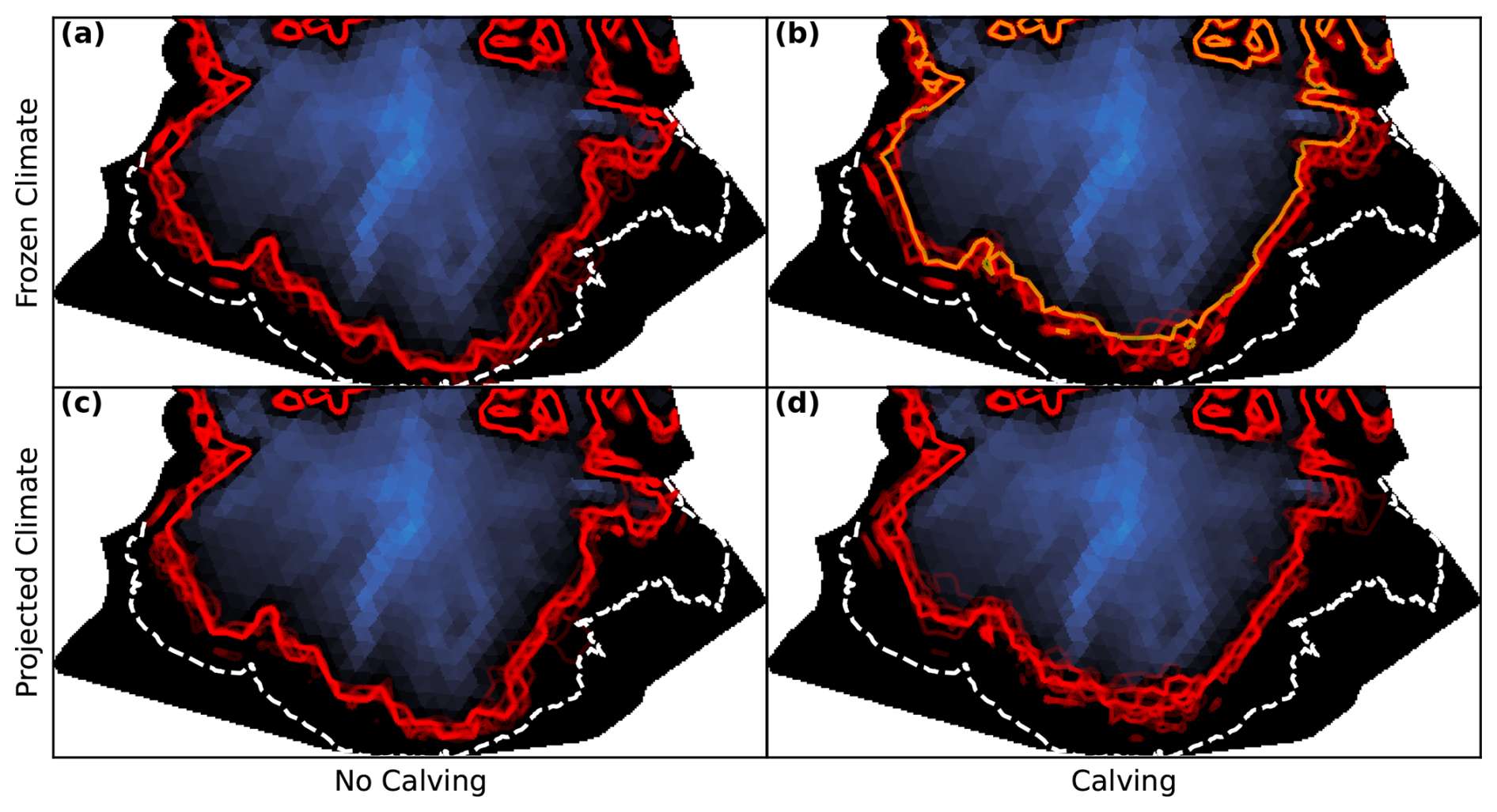
Figure 11 Predicted ice extent at 2073 under different assumptions of calving and projected surface mass balance. Red lines indicate terminus positions of individual ensemble members. The dashed white line indicates the ice extent circa 2023. The orange line corresponds to an ancillary experiment with fixed traction.

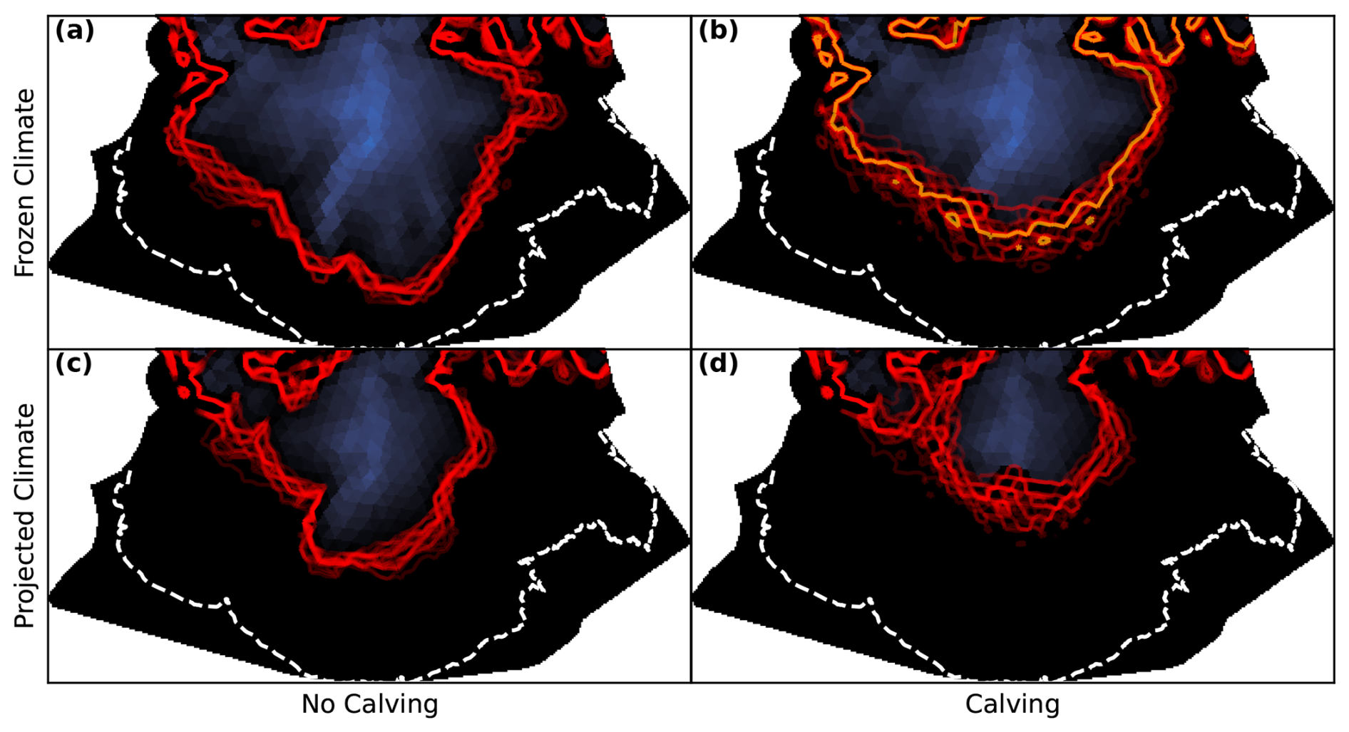
Figure 12 Predicted ice extent at 2173 under different assumptions of calving and projected surface mass balance. Red lines indicate terminus positions of individual ensemble members. The dashed white line indicates the ice extent circa 2023. The orange line corresponds to an ancillary experiment with fixed traction.

6.4 Forecasted change

Figure 10 shows the evolution of ice thickness from 1915–2023. At the beginning of this hindcast period, we see Sít' Tlein in a relatively extended configuration, with an oceanic interface where the ice extended past the top of the contemporary foreland. While we did not use historic observations of early 20th-century ice extent as a constraint, the model's inferred configuration in 1915 is in good qualitative agreement with maps from this time period (Russell, 1893; Tarr and Martin, 1914). In 2023, the ice extent and geometry match the present configuration by design. Figures 11 and 12 show the ice extent and thickness of the piedmont lobe in 2073 and 2173 under each combination of assumed calving and assumed future mass balance. Fifty years from present, we forecast with high probability that Sít' Tlein's lobe will disengage from the foreland and will terminate in a lake or marine embayment of increasing size. This modeled configuration is qualitatively similar to the contemporary state of neighboring Bering Glacier, which may serve as a valuable analog (Lingle et al., 1993). The qualitative differences between scenarios are minimal, although the presence of calving and a warmer climate both lead to slightly increased retreat. With respect to the latter, while the surface mass balance rate at high elevations differs by less than 0.1 m a⁻¹ (5 % of contemporary value), the difference in surface mass balance at sea level is approximately 2 m a⁻¹ (40 % of contemporary), yet the integrated effect of this difference over 50 years (a difference of around 50 m of total ablation at sea level, with smaller effects at higher locations) remains modest relative to the ice thickness. The differences in scenarios at 150 years from present are more dramatic; under linearly projected warming, Sít' Tlein's piedmont lobe will likely have mostly disintegrated, which is exacerbated by calving. Under a frozen climate, the piedmont lobe persists, albeit with a volume reduction of between 80 % and 90 %, depending on calving dynamics. At this time the surface mass balance at sea level is projected to be around 10 m a⁻¹, which is present twice. In the event that current forelands degrade in the absence of active glacier sedimentation, it could be the case that Seward Glacier will terminate in a shallow marine embayment, not dissimilar to neighboring Hubbard Glacier. However, the Sít' Tlein complex's geometry is not conducive to further retreat up its tributary fjords, which have beds that are likely above sea level, a contrast to Hubbard Glacier.

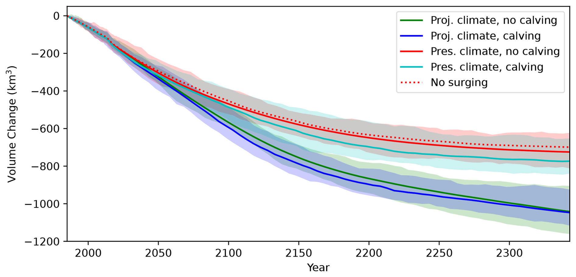
Figure 13 Volume evolution trajectories of Sít' Tlein from 1985 until 2344, with cyan and red corresponding to experiments with calving off or on, respectively, in which the surface mass balance is frozen at inferred 2023 values, and with green and blue corresponding to experiments with calving off or on, respectively, in which the surface mass balance is linearly extrapolated into the future. The dotted line corresponds to an ancillary experiment with fixed traction. Shaded regions correspond to 95 % credible intervals for each scenario.

Figure 4b and c show forecasted geometry along-profile along the red curve in Fig. 10b under both linearly extrapolated and steady-at-2023 climate assumptions. As expected, the frozen climate exhibits less retreat, particularly at 2173 (also see Figs. 11 and 12). However, the qualitative description in the previous paragraph applies to both cases; even if warming does not increase beyond present values, Sít' Tlein will likely undergo a disintegration of the piedmont lobe by 2173, changing from a mostly terrestrial terminus to a dominantly lacustrine or marine one. Over the 50-year scale, we expect modest surface lowering in the accumulation area under any scenario. However, 150 years from present under continuing warming, we see nearly double the surface thinning compared to the frozen experiment. In both cases the magnitude of changes in the accumulation area are smaller and less certain than those in the ablation zone. In summary, mass loss over the piedmont is largely already committed due to warming that occurred prior to 2023, whereas potential changes in the accumulation zone are still largely dependent on the degree to which climate changes in the future.

Finally, Fig. 13 provides the distribution of volume change for each experiment as a function of time. The influence of calving is small for the linearly extrapolated climate; the surface mass balance forcing is so strong that calving plays only a transient role in determining the mass evolution of the system. For the frozen climate experiment, scenarios including calving produce greater mass loss on average. However, such simulations are also more uncertain, as calving interacts nonlinearly with different random bed topographies. For all scenarios, the mass loss 50 years from present is similar, with a fixed climate (and marginalized over calving assumption) producing a mass loss with a 95 % credible interval of 323–444 km³ and a projected climate producing 383–505 km³. Because much of this ice is already below sea level, this translates into somewhat less than 1 mm of sea level equivalent. In 150 years from present, the frozen and projected climates produce 546–728 and 740–900 km³, respectively. In 300 years from present the variability is much greater, and the range of ice loss over the fixed climate scenarios is 600–820 and 920–1150 km³ for projected climate. In all scenarios, this corresponds at least to a disintegration of the piedmont lobe and perhaps further mass loss in the erstwhile accumulation area.

7 Discussion

7.1 The influence of surging

A conspicuous feature of Sít' Tlein is its surge cycle, which generates its characteristic looped moraines. The prominent geomorphological influence of these surges might suggest that such dynamics play a critical role in determining glacier shape and long-term dynamics. Indeed, such a hypothesis leads us to formulate a modeling framework that could capture the surge cycle. However, it was also not clear a priori whether surges influence glacier response to warming.

To evaluate this question, we performed a simple ancillary experiment in which – keeping all other variables fixed – we repeated the present climate with a calving ensemble but with β(x,t) fixed to its inferred temporal mean. We chose to maintain calving because its nonlinear interaction with velocity might serve to magnify the effect of surging, and we chose to use the present-day climate experiment because the relative importance of ice dynamics relative to the climate signal is higher. The resulting mean extents in 2073 and 2173 are overlain in Figs. 11 and 12, and the volume is shown in Fig. 13. In short, we find that the time-varying traction contributes little to Sít' Tlein's long-term dynamics. This is perhaps not surprising given that the continuity equation integrates the flux divergence through time just as it does the climate; in this context, surging appears as noise relative to the mean velocity, and this noise tends to average out over glaciologically relevant length scales.

7.2 The influence of basal sedimentation and alternate hypotheses for surface elevation change

Another similarly conspicuous feature of Sít' Tlein is its lack of mass loss through calving due to the presence of a large sedimentary morainal bank of varying composition (Thompson et al., 2024). As such, it is reasonable to imagine sedimentation playing a role in potential stabilization of the Sít' Tlein lobe as it undergoes tidewater retreat. To test this hypothesis, we perform a supplementary experiment in which we modify the basal topography such that the elevation of the bed at any location where it is both below sea level and not in contact with the ice base (in other words the ice has retreated away from the location) is raised either to the ice base or to sea level. Thus this experiment represents a maximal sedimentary end-member where there is an infinite supply of sediment that is deposited instantly wherever possible. We apply this experiment to the present-climate case without calving, which would lead to the greatest potential influence for proglacial sedimentation (Brinkerhoff et al., 2017).

The resulting glacier evolution is effectively identical to the experiment without sediment dynamics. This lack of sensitivity is again a result of the basic conclusion that the contemporary lobe extent is incompatible with current climate; the retreat is driven by a surface mass imbalance, and as such modification of losses to calving have little influence.

Despite the small modeled influence of sedimentation under this simplified case, Sít' Tlein's current morphology is undoubtedly controlled by the presence of its terminal moraine. Indeed, in the absence of a protective moraine, it is unlikely that Sít' Tlein could have advanced to its current position, and thus it is possible also that Sít' Tlein undergoes tidewater glacier periodicity (Meier and Post, 1987), in which slow sediment-driven advances are punctuated by fast retreats from extended positions. This leads to an alternative or augmenting hypothesis for contemporary surface lowering at Sít' Tlein, namely that the observed surface elevation change signal may be a result not of ice thinning, but rather of fluvial erosion of underlying sedimentary structures. Indeed, observations from nearby Taku Glacier show that contemporary surface lowering rates over the lobe are not inconsistent with observations of the erosion of subglacial sediment (Motyka et al., 2006). Furthermore, Sít' Tlein has exhibited asynchronous retreat relative to its neighbors such as Hubbard Glacier, which retreated and began re-advancing in the early 19th century, and the collective terminus of Tsaa, Guyot, Yahtse, and Tyndall glaciers, which filled contemporary Icy Bay and began a retreat towards its present configuration around the turn of the 20th century. Such asynchronicity implies that climate forcing alone may not be the sole factor in determining its retreat. On the other hand, observed surface elevation change is relatively consistent across the Sít' Tlein lobe, including over subglacial canyons that are unlikely to be of sedimentary origin, which implies that bed elevation changes cannot be responsible for surface lowering there. Detailed exploration of tidewater glacier periodicity in a large system such as Sít' Tlein and its neighbors via coupling of a realistic model of glacier evolution such as this one to a sediment dynamics model as in Brinkerhoff et al. (2017) remains an avenue for future work; however, we think it likely that the contemporary configuration of St. Elias Range glaciers broadly reflects long timescale sedimentary processes driving natural variability, on top of which a strong contemporary warming signal is superimposed.

7.3 Landscape-scale effects

Our results imply that the continued existence of Sít' Tlein's piedmont lobe is inconsistent with contemporary climate forcing, let alone forcing subject to continued warming. As such, this system will, over the next century, undergo a landscape-scale transition from a terrestrially terminating system grounded on a broad array of ice- and non-ice-cored moraines into a lake- or ocean-terminating one, presumably with a new calving front. The degree to which the resulting system will resemble Bering Glacier to the west, which terminates into a primarily freshwater lake, or Hubbard Glacier to the east, which terminates into a saltwater bay, depends on the potential degradation of the Sít' Tlein forelands.

In either case, the local ecosystem has the potential for substantial change. In the near term, enhanced melting and disintegration of the piedmont lobe will lead to an increase in freshwater flux into the Gulf of Alaska. From an oceanographic perspective, such fluxes are a primary driver of coastal circulation, while reduced salinities control along-shore currents resulting from density gradients (Neal et al., 2010). Such modifications to the local biogeochemistry can also have impacts on primary productivity for phytoplankton and the various species that feed on it at various trophic levels, including salmon and marine mammals. From the perspective of physical habitat, the opening of a new coastal bay will also have implications on the presence of wildlife. Presumably the disintegration of the forelands will have deleterious effects on local terrestrial ecosystems, including forests growing upon ice-cored moraines and the wildlife populations – such as brown bears – that use them, whereas the increased availability of ice-berg-rich waters will provide a new habitat for marine mammals such as harbor seals (Blundell et al., 2011). One major impact of piedmont lobe degradation will be the conversion of the terrestrial glacierized landscape – which is part of Wrangell–St. Elias National Park and Preserve – into unprotected marine waters. This could constitute the largest removal of park lands in the history of the National Park System. It is not yet clear what the other potential impacts on human uses, including subsistence use, will be.

7.4 Model limitations

The model ensemble presented here represents our best effort to produce a credible prediction of future change at Sít' Tlein, including both a defensible representation of uncertainties and demonstrable skill at hindcasting. However, it still possesses limitations that should be considered when contextualizing these results.

7.4.1 Geometry models

First, our prior distribution over the bed elevation is simplistic relative to the true richness of the region's geomorphic reality. While convenient and flexible, a Gaussian process with fixed kernel parameters cannot capture the effects of the full range of geomorphological processes acting in this region, especially the qualitative difference between the topography that is currently beneath the ice (which is relatively muted and smooth) versus the subaerial topography comprising the St. Elias range's dramatic aretes and peaks (Cotton et al., 2014). In particular, our terrain model is in many places too smooth, while in others it is too rough. Terrain models that rely on an adaptive basis, for example using generative adversarial networks trained on natural topography, might present an alternative (Voulgaris et al., 2021). However, a fundamental challenge remains in that the effective dimensionality required to represent spatial variability increases with decreasing spatial regularity, which is particularly challenging when trying to compute posterior covariance matrices. A similar criticism is reasonable for the basal traction, though we have little basis for understanding the spatial correlation structure for traction given that it is not directly observable.

Finally, our spatial discretization of the model physics is fairly coarse, which was necessary for computational efficiency. We performed some qualitative experiments to assess the impact of this. In particular, we performed the time-independent phase of the MAP estimation using a mesh with nominal 750 m resolution. We also ran one member from each of the ensemble experiments above with this high-resolution mesh (using parameters inferred from the lower-resolution version). In each case, we did not find major qualitative differences. However, this does not constitute a full-convergence analysis, and the influence of higher-resolution meshes remains a topic of future study.

7.4.2 Spatial parameterization of surface mass balance

As emphasized previously, a critical limitation is our use of a simple parameterization of surface mass balance, which reflects our lack of detailed process understanding. This model is perhaps inadequate in several ways, particularly when taken in conjunction with our general lack of knowledge about the spatial distribution of accumulation and melt in the St. Elias range. First, we assume surface mass balance to vary with elevation according to a piecewise linear function with change points defined at sea level, the ELA, the median elevation of the principle accumulation zone, and the highest elevation. This captures some phenomenological features that are observed and that also sometimes show up in other models. For instance, such a model can represent the different relationship between surface mass balance below and above the ELA induced by differing physical processes of melting ice versus snow (which appear as differing degree day factors in temperature index models;  Hock and Holmgren, 2005). It also parameterizes the typical rarefaction of precipitation at very high elevations. Nonetheless, despite including the capacity for explicit spatial variation, we do not believe that this parameterization fully captures the region's dramatic orographic effects like rain shadowing, topographic steering of precipitation, or the influences of solar aspect. Critically, this parameterization also does not take into account the influence of debris mantling, which could have an impact in the near-terminus region. Indeed, in some regions near the ice terminus, sufficient material has accumulated to support a rich plant community (including trees), and melt has essentially stopped. In such regions, the semantic distinction between glacial ice and ice-cored moraine also becomes somewhat ambiguous. Regardless of such definitions, we lack validated models both for predicting debris thickness and for estimating its influence on melt rates.

7.4.3 Temporal parameterization of surface mass balance

Similarly, the variation in surface mass balance in time is parameterized solely as a linear trend (and random interannual variability), which ignores potential knowledge of local and global temperature and precipitation trends – although the extrapolation of such knowledge at Sít' Tlein represents a challenge. Nonetheless, a better approach that could deal with both of these simplifications might be to use a high-resolution regional climate model (e.g., Bieniek et al., 2016) – perhaps in conjunction with linear orographic precipitation theory (Smith and Barstad, 2004) to accommodate additional topographic detail – to derive time-varying precipitation alongside a surface energy balance model (e.g., Hock and Holmgren, 2005) to estimate melt. However, such models have many parameters themselves and are not easily amenable to integration within an automatic differentiation framework. Combined with the paucity of observations for the glacial system considered here, it is not clear that the resulting more sophisticated model would lead to an increase in predictive skill, and high-quality surface mass balance modeling in mountains remains an active research area.

7.4.4 Ice–ocean interactions

Our model makes use of a simplified frontal ablation parameterization, and we explore two representative configurations of such physics: one in which frontal ablation does not occur and one in which it occurs at a rate similar to a previously observed tidewater retreat. Nonetheless it is possible that this simplified approach could miss more nuanced processes. For example, our model does not explicitly account for the intrusion of warm, oceanic saltwater, which we know to be occurring at Sitkagi Lagoon and not at Malaspina Lake (yet, to our knowledge). As such, the details of potential tidewater retreat – particularly during early stages in which the glacier is still interacting with its terminal moraine – might not be fully captured. Nonetheless, because the primary driver of the surface elevation change at Sít' Tlein is very likely to be a profound surface mass imbalance, we believe that these inaccuracies are unlikely to modify the longer-term conclusions presented here regarding the stability of the piedmont lobe (as is indicated in Fig. 13).

7.4.5 Models of observational uncertainty

Finally, with respect to the inference procedures described here, we make use of simplified models of measurement noise for all observed quantities. While we make heavy use of normal distributions to model noise in all of our datasets, it is very likely the case that all observations are biased in complicated (and unmodeled) ways and also that the uncertainty characteristics admit outliers. We do not have a good understanding of observational uncertainty for most products even when provided. Even if we had a detailed understanding of marginal error statistics (i.e., the observational uncertainty in surface velocity at a single point), spatial and temporal correlations in error are unreported and unknown. While we have tried to be conservative in defining our likelihood models, it is undoubtedly the case that we have induced additional model error through misspecification of such likelihoods.

7.5 Methodological contribution of this paper

The current paper combines methodological advances developed over several decades of research in glaciological inverse problems. The linchpin is an adjoint model for ice flow which allows for the efficient computation of gradients of model inputs with respect to outputs. Adjoint models, introduced by MacAyeal (1993), have become a workhorse for practical ice sheet modeling, variously being used to determine traction and/or rheological parameters (Joughin et al., 2004; Morlighem et al., 2013; Sergienko and Hindmarsh, 2013; Habermann et al., 2013; Petra et al., 2014; Isaac et al., 2015; Arthern et al., 2015; Riel et al., 2021; among others).

The simultaneous inference of multiple fields, as we do in this paper, has been explored previously; for example, Gudmundsson and Raymond (2008) simultaneously inferred traction and bed geometry from surface expressions using a transfer function approach. Petra et al. (2012) inverted for both the rheological prefactor and traction coefficient, while Gudmundsson et al. (2019) performed a similar inversion across the whole of Antarctica. Ranganathan et al. (2021) invert for the traction coefficient and rheological prefactor over ice streams in Antarctica, developing a specialized regularization approach in hopes of finding a unique partitioning between parameters. Here, our parameters represent not only the basal traction and topography, but surface mass balance as well. This simultaneous inference is essential to producing a model that is free of spurious transient dynamics – after all, the configuration of a real glacier represents the long-term integration of ice motion, thickness, and surface mass balance at once, and we have endeavored to reproduce numerically that same physical self-consistency. Of particular relevance, Perego et al. (2014) inverted simultaneously for traction and bed geometry so as to match velocities and also produce an ice sheet initial condition free from spurious transients.

One way that our work departs from most adjoint-based data assimilation methods is its integration of temporal observations in an explicitly time-dependent fashion. Goldberg and Heimbach (2013), in perhaps the first application of a time-dependent adjoint to inverse problems in glaciology, simultaneously inferred traction and bed geometry for a synthetic case from time-dependent observations of surface velocity and elevation; these methods were extended to state-consistent modeling of several glaciers in West Antarctica (Goldberg et al., 2015). Similarly, Larour et al. (2014) combined a spin-up process with the inference of time-dependent surface mass balance and traction fields conditioned on surface elevation and surface velocity observations for the Northeast Greenland Ice Stream, also employing a time-dependent adjoint. Choi et al. (2023) recently applied a time-dependent adjoint to a time series of velocity observations in Greenland. We follow in the footsteps of these works but apply their ideas to a broader set of parameters and observations. A novel aspect of our model with respect to implementation is its integration within the general purpose automatic differentiation tool Pytorch (Paszke et al., 2019), which allows for seamless access to complex linear algebra operations and differentiation through time. We have used this tool for the particular purpose of determining a set of optimal model parameters via gradient-based optimization through time (and their associated uncertainty quantification); however, it is quite general and could be used to infer other parameters or establish sensitivities of different quantities of interest with little modification, particularly because the integration with Pytorch makes it straightforward to compute gradients of other non-misfit functions with respect to model inputs (for example, the sensitivity of future grounding line flux with respect to initial conditions).

Allowing multiple parameters to vary at once also leads to ambiguity in their inferred values – is a particular observed surface velocity the result of thick ice moving mostly via deformation or thin ice that is sliding faster? As such, we view at least an approximation of posterior covariance between potentially equifinal parameters as essential. To this end, building on previous works we utilize a well-known method – the Laplace approximation – to derive the uncertainty over inferred parameters. In particular, Isaac et al. (2015) adapted the methods of Bui-Thanh et al. (2013) to the ice sheet context, developing the methodology for the low-rank Laplace approximation to the posterior covariance that we employ in this work. Such methods have been extended a few times since; Koziol et al. (2021) used a similar approach to perform a snapshot inversion with estimated posterior covariance of traction for a synthetic case but also propagated the resulting uncertainty forward through time. Recinos et al. (2023) extended these methods to three West Antarctic ice streams. Here we apply this framework to a diverse set of spatiotemporal observations and in conjunction with a higher-order time-dependent model with both changing velocity and geometry, a first in both cases. More broadly the methodological advances here provide a framework for the creation of ice flow model predictions that accommodate a broad range of observational constraints (and that produce hindcasts that agree with time-dependent observations) while remaining robust to the absence of unknown inputs and quantifying the resulting induced uncertainties.

The inclusion of time-dependent inference and uncertainty quantification is not without cost, and both of these factors lead to significantly increased computational expense relative to a time-static and deterministic inversion. With respect to the former, every evaluation of the likelihood elicits evaluation of the model over the observational period (and perhaps beyond, as in our case). This cannot be reduced because the model must produce a prediction at every time for which data exist. However, it may be possible to accelerate models via emulation, particularly of the stress balance solver as in Jouvet et al. (2022), although it remains to be seen whether such models are sufficiently robust to handle the diversity of flow conditions in systems such as Sít' Tlein. With respect to uncertainty quantification, both the randomized Laplace approximation and simple Monte Carlo forecasting that we employ here are embarrassingly parallel, a key advantage for computational tractability, particularly given the widespread availability of compute cores in the cloud. We emphasize, however, that such expense is unavoidable for credible modeling of data-limited systems such as Sít' Tlein.

Nonetheless, the amount of computation needed to accurately characterize inferred parameters of our predicted quantities of interest scales with the complexity of the problem, and application of these methods to larger systems like Greenland or Antarctica may be much more expensive. However, we have been careful – particularly in our construction of parameter representations – to take advantage of approximate sparsity and low-rankness, and we believe that our approach is still reasonable at the ice sheet scale; for reference, the complete computational pipeline for this work took around 20 h using one eight-core i9-13900HX processor. The bulk of this time (60 %) was spent computing Hessian vector products, while 20 % was spent computing the projection ensemble. As mentioned previously, both of these tasks are trivial to parallelize and would see a linear speedup with the addition of computing power.

8 Conclusions

Sít' Tlein, the world's largest piedmont glacier, will with high probability undergo a transformation over the next century as its low-elevation piedmont lobe disintegrates and transitions into a lake or marine terminating glacier. This conclusion is supported by data-constrained probabilistic ice flow modeling. We used spatiotemporal observations of velocity, radar observations of the glacier bed, a diverse time series of surface elevations, and sparse observations of specific surface mass balance to inform a joint probability distribution over the critical parameters of the 𝖲𝗉𝖾𝖼𝖤𝖨𝖲 ice flow model. Because the system is high-dimensional and the model expensive to evaluate, we apply a number of existing and novel tools to render the problem tractable: the integration of the time-dependent model with the general purpose automatic differentiation tool Pytorch, careful finite-dimensional representations of model parameters, and low-rank Laplace approximation to the posterior covariance. Our model exhibits very good agreement with observations over the historic record. We then sampled from parameter distributions to drive a model ensemble characterizing Sít' Tlein's future evolution over 4 centuries. While there is spread in total mass loss (between 600 and 1300 gt at 300 years from present), we find the vulnerability of Sít' Tlein's piedmont lobe to be robust to variations in forcing, parameters, and model structure.

Appendix A: Discretization

𝖲𝗉𝖾𝖼𝖤𝖨𝖲 discretizes in space using a mixed finite-element method. Finite-element methods represent spatial functions as a linear combination of fixed basis functions that are defined on a mesh, which we take here to be a triangular tessellation of the model domain (Fig. 1b); each triangle in the mesh is called a cell, and in SpecEIS we represent the thickness field as a weighted sum of cell-wise constants (e.g., as a function in the zero-order discontinuous Galerkin space, hereafter abbreviated DG0; Boffi et al., 2013).

$$\begin{array}{}\text{(A1)}& H(\mathit{x},t)\approx \sum _{k\in \left|\mathcal{T}\right|}{\mathit{\varphi }}_k\left(\mathit{x}\right){\mathsf{H}}_k\left(t\right),\end{array}$$

where 𝒯 is the set of mesh cells,

$$\begin{array}{}\text{(A2)}& {\mathit{\varphi }}_k\left(\mathit{x}\right)=\left\{\begin{array}{l}\mathrm{1}\mathrm{if}\mathit{x}\in {\mathcal{T}}_k\\ \mathrm{0}\mathrm{else},\end{array}\right.\end{array}$$

and 𝖧_k(t) is the time-varying thickness coefficient, which here can reasonably be interpreted as the average thickness across mesh cell k. The velocity is similarly represented as a weighted sum of basis functions

$$\begin{array}{}\text{(A3)}& \mathit{u}(\mathit{x},z,t)\approx \sum _{k\in \left|\mathcal{E}\right|}\sum _{l=\mathrm{1}}^{\mathrm{3}}{\mathit{\psi }}_{kl}\left[{\stackrel{\mathrm{‾}}{\mathsf{U}}}_{kl}+{\displaystyle \frac{{\mathsf{U}}_{kl}^{\prime }}{n+\mathrm{1}}}\left(\right(n+\mathrm{2}){\mathit{\varsigma }}^{n+\mathrm{1}}-\mathrm{1})\right],\end{array}$$

where ℰ is the set of mesh edges, ψ_kl(x) is the lth Mardal–Tai–Winther basis function (of which there are three per edge; Mardal et al., 2002) associated with the kth edge, and ${\stackrel{\mathrm{‾}}{\mathsf{U}}}_{kl}$ and ${\mathsf{U}}_{kl}^{\prime }$ are coefficients associated with the depth-averaged and depth-varying components of the ice velocity (the monolayer higher-order approximation; Dias dos Santos et al., 2022). In contrast to the thickness discretization, these velocity coefficients represent the magnitude of the velocity field normal and tangential to cell edges. This combination of finite elements generalizes the so-called Arakawa staggered C-grid (Arakawa and Lamb, 1977) that is frequently used for shallow-ice models to correctly account for the longitudinal stresses of the Blatter–Pattyn approximation and is known to maintain thickness positivity and uphold mass conservation while being free from spurious numerical wiggles. SpecEIS discretizes in time using the backward Euler method applied simultaneously to both equations and as such is fully implicit. The resulting nonlinear system of equations is solved using a damped Picard iteration. A detailed description of this model, as well as a full suite of experiments quantifying and verifying model performance, is found in Brinkerhoff (2023).

Internal to the model, we maintain a finite-element representation of the parameters m. H₀(x) is represented identically to H(x,t), and we refer to its coefficients as 𝖧₀. The surface mass balance and bed elevation are also represented using the DG0 space, with coefficients $\dot{\mathsf{a}}$ and 𝖡, respectively. In contrast, the basal traction uses a first-order continuous Galerkin (piecewise linear, CG1) basis with coefficients β associated with a nodal basis.

We discretize the contributing area of Sít' Tlein at a relatively coarse 1.5 km horizontal resolution. The resulting mesh has 3898 cells, 1997 nodes, and 5824 edges. While it is possible in this framework to adapt mesh element sizes with respect to a desired criterion (commonly velocity magnitudes, strain rate magnitudes, or grounding line proximity), we expect both the velocity and geometry to change significantly over the course of our simulations, so we opt for a nearly uniform element size distribution under the assumption that this mesh is of sufficient resolution to capture the glacier's essential features.

Appendix B: Gradients via the adjoint method

The adjoint method aims to efficiently compute the gradient of a cost function ℒ(𝖵,𝗆) with respect to parameters $\mathsf{m}=[{\mathsf{H}}_{\mathrm{0}},\mathsf{B},\mathit{\beta },\mathsf{a}]$, where $\mathsf{V}=[H,\stackrel{\mathrm{‾}}{\mathsf{U}},{\mathsf{U}}^{\prime }]$ is the vector of state variables. We begin by writing a new constrained cost function

$$\begin{array}{}\text{(B1)}& \mathcal{J}\left(\mathsf{m}\right)=\mathcal{L}[\mathsf{V};\mathsf{m}]+\mathcal{A}[\mathit{\lambda },\mathsf{V};\mathsf{m}],\end{array}$$

where $\mathcal{A}[\mathit{\lambda },\mathsf{V};\mathsf{m}]$ is the constraint, and $\mathit{\lambda }=\left[{\mathit{\lambda }}_{\mathrm{1}},{\mathit{\lambda }}_{\mathrm{2}}\right]$ represents Lagrange multipliers. The constraint here is the semi-discretized weak form of the coupled forward model (Eqs. 5 and 7)

$$\begin{array}{}\text{(B2)}& \begin{array}{rl}\mathcal{A}[\mathit{\lambda },\mathsf{V};\mathsf{m}]& =\underset{\stackrel{\mathrm{‾}}{\mathrm{\Omega }}}{\int }{\mathit{\lambda }}_{\mathrm{1}}\left({\displaystyle \frac{H_{k+\mathrm{1}}-H_k}{\mathrm{\Delta }t}}-{\dot{a}}_{k+\mathrm{1}}\right)\mathrm{d}A\\ & +\underset{\partial \stackrel{\mathrm{‾}}{\mathrm{\Omega }}}{\int }\left[{\mathit{\lambda }}_{\mathrm{1}}{\mathit{n}}_{\mathit{x}}\right]\cdot \widehat{\stackrel{\mathrm{‾}}{\mathit{u}}H}\mathrm{d}s,\\ & +\underset{{\mathrm{\Gamma }}_{out}}{\int }\left({\mathit{\lambda }}_{\mathrm{1}}{\mathit{n}}_{\mathit{x}}\cdot {\stackrel{\mathrm{‾}}{\mathit{u}}}_{k+\mathrm{1}}{H}_{k+\mathrm{1}}\right)\mathrm{d}s\\ & -\underset{{\mathrm{\Omega }}_T}{\int }{\mathrm{\nabla }}_{\mathit{x},z}{\mathit{\lambda }}_{\mathrm{2}}:\left(\mathrm{2}{\mathit{\eta }}_{k+\mathrm{1}}{H}_{k+\mathrm{1}}{\dot{\mathit{ϵ}}}_{\mathrm{1},k+\mathrm{1}}\right)\mathrm{d}V\\ & -\underset{{\mathrm{\Omega }}_T}{\int }{\mathit{\rho }}_{i}g\left[{\mathrm{\nabla }}_{\mathit{x}}\cdot \left({\mathit{\lambda }}_{\mathrm{2}}{H}_{k+\mathrm{1}}\right)\right]S_{k+\mathrm{1}}\mathrm{d}V\\ & -\underset{{\stackrel{\mathrm{‾}}{\mathrm{\Omega }}}_T}{\int }{\left[{\mathit{\beta }}_{t+\mathrm{1}}^{\mathrm{2}}{N}_{t+\mathrm{1}}^p\Vert \mathit{u}{\Vert }_{k+\mathrm{1}}^{m-\mathrm{1}}({\mathit{\lambda }}_{\mathrm{2}}\cdot {\mathit{u}}_{\mathit{k}\mathbf{+}\mathbf{1}})\right]}_{\mathit{\varsigma }=\mathrm{1}}\mathrm{d}A\\ & -\underset{{\mathrm{\Gamma }}_W}{\int }\mathit{\alpha }(\mathit{u}\cdot {\mathit{n}}_{\mathit{x}})({\mathit{\lambda }}_{\mathrm{2}}\cdot {\mathit{n}}_{\mathit{x}})\mathrm{d}s\\ & -\underset{\partial \mathrm{\Omega }}{\int }{\mathit{\rho }}_{i}g\left[{\mathit{n}}_{\mathit{x}}\cdot {\mathit{\lambda }}_{\mathrm{2}}{S}_{k+\mathrm{1}}\right]\mathit{\left\{}{H}_{k+\mathrm{1}}\mathit{\right\}}\mathrm{d}A,\end{array}\end{array}$$

where we have used integration by parts to substitute natural boundary conditions and in which jump, average, and numerical flux terms appear due to the discontinuous Galerkin discretization of the thickness field. A full description of the above manipulations can be found in Brinkerhoff (2023).

We seek to compute the gradient with respect to the parameters by eliminating the state variables and Lagrange multipliers. Taking the first variation (i.e., the Gateaux derivative) of Eq. (B1) with respect to the (basis expansion of the) Lagrange multiplier in the direction of a test function and setting the result to zero recovers the weak form of the forward model, which can be solved via finite elements as usual. Taking the first variation with respect to the (basis expansion of the) model state variables in the direction of a test function and equating the result with zero yields a weak form of the adjoint equation, with the right-hand side given by $\frac{\partial \mathcal{L}}{\partial V}$, the derivative of the cost with respect to the forward model's output and precisely the quantity delivered by reverse mode automatic differentiation.

The adjoint equation is structurally similar to the forward equation, with both an adjoint transport equation (which propagates misfit information opposite in time and spatial direction relative to the forward model) and an adjoint stress balance equation (which has a more complex viscosity term). The adjoint equations are linear in λ and can be solved with finite elements using similar methods to the forward model.

With forward and adjoint systems solved, the gradient terms can be readily computed by taking the Gateaux derivative of Eq. (B1) with respect to m in the direction of suitable test functions. The resulting expressions will generally depend on both λ and 𝖵 and can be evaluated to find the desired derivatives in terms of the basis coefficients $\frac{\partial \mathcal{L}}{\partial \mathsf{m}}$, which can be used directly or – as in our case – propagated further back in the computational graph to compute gradients of the cost with respect to the arguments of the functions used to form 𝗆. We do not calculate the analytical representation of either the adjoint equation or gradient expressions by hand, instead relying on the symbolic differentiation capabilities of Firedrake.

Appendix C: Representations of model parameters

C1 Bed elevation

We parameterize the probability distribution over the bed elevation as a Gaussian process (GP; Williams and Rasmussen, 2006, from whom we also adopt notation) in space, which assumes that the function value at any two coordinates x and x^′ are jointly normal, with a covariance given by a kernel function $k(\mathit{x},{\mathit{x}}^{\prime })$ and mean function m(x). Throughout this and the following sections, we use this notation frequently for different parameters and do not differentiate between them for concision of presentation. We hope that which parameter we refer to is clear from context. Evaluated at a finite set of spatial points $\mathbf{X}\in {\mathbb{R}}^{n\times \mathrm{2}}$ (for example, the finite set of observation locations or the quadrature points of a finite-element mesh), we can describe the distribution over this function with a normal distribution

$$\begin{array}{}\text{(C1)}& P\left(B\right(X\left)\right)=\mathcal{N}(\mathit{\mu },\mathbf{K}),\end{array}$$

where $K\in {\mathbb{R}}^{n\times n}$ is the covariance matrix $K_{ij}=k(X_i,X_j)$, and $\mathit{\mu }=m\left(X\right)\in {\mathbb{R}}^n$ is the mean vector. While unrealistically simplistic for representing the extreme and glacierized topography of the St. Elias range, we nonetheless use the Matern family of covariance functions. The behavior of the distribution is governed by a length scale, amplitude scale, and differentiability index. At Sít' Tlein, based on maximum marginal likelihood estimation (Tober et al., 2023) we take the characteristic length scale l as 3 km, the differentiability $\mathit{\nu }=\frac{\mathrm{3}}{\mathrm{2}}$, and the amplitude to be 1000 m. We model the distribution over the mean function as a polynomial

$$\begin{array}{}\text{(C2)}& m\left(\mathit{x}\right)=\mathit{h}(\mathit{x}{)}^T\mathit{\alpha },\end{array}$$

where h is a set of orthogonalized degree-two polynomial basis functions, and α is a coefficient vector. Taken together this model assumes that the topography is well approximated by a quadratic polynomial with local variability given by a GP.

C1.1 Low-rank decomposition

K is often low-rank, which is to say that some of its columns contain redundant information (for example when points in X are close together relative to the characteristic length scale of the GP). This property motivates a reparameterization of P(B) as

$$\begin{array}{}\text{(C3)}& B\left(X\right)=\mathbf{L}\mathit{w}+H\mathit{\alpha },\mathit{w}\sim \mathcal{N}(\mathrm{0},I),\mathit{\alpha }\in {\mathbb{R}}^{\mathrm{6}},\end{array}$$

where $\mathbf{H}=\mathit{h}\left(X\right)\in {\mathbb{R}}^{n\times \mathrm{6}}$ is a Vandermonde matrix, and $\mathbf{L}\in {\mathbb{R}}^{n\times r}$ is an approximate root of the spatial covariance matrix such that LL^T≈K. Note that L need not be square; if K is indeed low-rank, then r may be much less than n. Under this reparameterization the degrees of freedom that characterize function behavior (and that need to be inferred in the inverse context) are the coefficients w∈ℝ^r, which are a priori unit-normal. Such a decomposition decouples the number of degrees of freedom necessary to represent the function (i.e., the length of w) from the number of locations at which this function is to be evaluated, a desirable property. B(X) under this choice of representation can be described as a combination of finite basis functions, and we refer to the matrix L as the basis for B(X).

C1.2 Structured kernel interpolation

We now turn to the construction of L(X). Many matrix decompositions produce an approximate matrix root; however, some choices are either intractable to compute, not low-rank, or have undesirable numerical properties. The classic choice is a (truncated) eigendecomposition; however, this has two issues. First, it requires the explicit construction, storage, and manipulation of the matrix K. While randomized methods can circumvent some of the problematic scaling associated with computing the decomposition, circumventing the storage requirement is challenging. Second, despite this decomposition optimally capturing the low-rank structure of the target covariance matrix, it does not retain the characteristics of the underlying matrix; even though K may be nearly sparse in the sense that the covariance between distant points is numerically zero, the associated basis has columns that are non-sparse. All things equal, we prefer a decomposition that retains the approximate sparsity of the original matrix.

Here we describe an approach that addresses both of these issues. In order to circumvent the requirement that we form the matrix K explicitly, we employ structured kernel interpolation (SKI; Wilson and Nickisch, 2015), which posits that the covariance matrix can be approximated as

$$\begin{array}{}\text{(C4)}& \mathbf{K}\approx \mathbf{W}({\mathbf{K}}^x\otimes {\mathbf{K}}^y){\mathbf{W}}^T,\end{array}$$

where K^x and K^y are 1D covariance matrices defined over regular grids in each map-plane dimension independently and W an interpolation matrix. The Kronecker product of the two 1D covariance matrices is then a 2D covariance matrix evaluated on regular grid. In this work, we take each of these 1D grids to extend a few length scales past the boundaries of our mesh in each dimension with a spacing of $l/\mathrm{10}$. The Kronecker product is not any easier to store explicitly; however, matrix–vector products can be efficiently computed by only forming each 1D covariance matrix independently.

This grid-evaluated covariance is not useful on its own; it provides correlations between function values at the wrong locations. To map this structured covariance to arbitrary locations X we employ an interpolation matrix W (in this work we use inverse distance weighting). W is highly sparse, with inverse distance weighting leading to only four non-zero entries per row (only the four grid points bounding the desired evaluation location contribute to the interpolation). As such the product of Eq. (C4) with an arbitrary vector can be evaluated inexpensively. The error induced by this interpolation is typically small (Wilson and Nickisch, 2015). Again, while computing the left side of Eq. (C4) is usually intractable, the computation and storage of each factor on the right side are straightforward, and their properties allow for the efficient computation of matrix–vector products.

We can also efficiently produce a matrix root. Again invoking the algebraic properties of the Kronecker product, we write

$$\begin{array}{}\text{(C5)}& \begin{array}{rl}\mathbf{K}& \approx L{L}^T\\ \mathbf{L}& =\mathbf{W}({\mathbf{L}}^x\otimes {\mathbf{L}}^y),\end{array}\end{array}$$

where L^xL^xT≈K^x and similarly for L^y. Concretely, rather than decompose the matrix directly, we perform a component-wise decomposition of separable Kronecker-factored covariance matrices (which are very small) and then sparsely interpolate these to evaluation points.

As a final step, we must select a low-rank decomposition for the coordinate-wise covariance matrices. We use the Nyström approximation applied to a matrix root to compute the low-rank factor

$$\begin{array}{}\text{(C6)}& {\mathbf{L}}^x={\mathbf{K}}_{[:,\mathit{p}]}^x{\mathbf{V}}^x{\mathbf{\Lambda }}^{x-\frac{\mathrm{1}}{\mathrm{2}}}{\mathbf{V}}^{xT}),\end{array}$$

where p represents the indices of pivot columns (here selected rigorously through pivoted QR decomposition) and where V^x and Λ^x are the eigenvectors and values of $K_{[\mathit{p},\mathit{p}]}^x$, respectively. The resulting factor's columns are basis vectors that resemble scaled entries in the covariance matrix – including the same sparsity patter – but where redundant columns have been eliminated. The resulting procedure yields a representation with 4192 degrees of freedom.

C1.3 Conditioning on bed observations

Next we turn to constraining bed elevations from direct observations. NASA's Operation IceBridge collected over 4000 km of 2.5/5 MHz radar soundings between 2013 and 2023, from which the glacier base can be interpreted with a nominal error of approximately 25 m based on integrated analysis at sounding crossover points. A detailed analysis of this product can be found in Tober et al. (2023). We combine these radar soundings – which are relevant for subglacial locations – with the Copernicus GLO-30 digital elevation model (European Space Agency, 2019) masked to ice-free regions to produce a combined dataset that provides observations of the bedrock elevation at varying degrees of spatial density across our study area. We assume that these observations are independent and normally distributed about the true bedrock elevation with an observational standard deviation σ_obs=25 m, or

$$\begin{array}{}\text{(C7)}& P\left(\widehat{B}\right|B\left({\mathbf{X}}_{\mathrm{obs}}\right))=\mathcal{N}(B\left({\mathbf{X}}_{\mathrm{obs}}\right),{\mathit{\sigma }}_{\mathrm{obs}}^{\mathrm{2}}\mathbf{I}),\end{array}$$

where ${\mathbf{X}}_{\mathrm{obs}}\in {\mathbb{R}}^{n_{\mathrm{obs}}\times \mathrm{2}}$ are the observation coordinates. We specify the coefficients of the mean function $\stackrel{\mathrm{‾}}{\mathit{\alpha }}$ by the standard least squares solution

$$\begin{array}{}\text{(C8)}& \stackrel{\mathrm{‾}}{\mathit{\alpha }}={\left({\mathbf{H}}_{\mathrm{obs}}^T{\mathbf{H}}_{\mathrm{obs}}\right)}^{-\mathrm{1}}{\mathbf{H}}_{\mathrm{obs}}^T\widehat{B},\end{array}$$

where H_obs=h(X_obs). Because both this likelihood and the prior distribution are normally distributed, and because the map from GP coefficients w to B is linear, the posterior distribution has an analytical solution given by

$$\begin{array}{}\text{(C9)}& {\displaystyle }\begin{array}{rl}P\left(\mathit{w}\right|\widehat{B},\mathit{\alpha })& =\mathcal{N}(\stackrel{\mathrm{‾}}{\mathit{w}},\mathbf{\Sigma })\\ \mathrm{\Sigma }& ={\left(\mathbf{I}+{\mathbf{L}}_{\mathrm{obs}}^T{\mathit{\sigma }}_{\mathrm{obs}}^{-\mathrm{2}}{L}_{\mathrm{obs}}\right)}^{-\mathrm{1}}\end{array}\text{(C10)}& {\displaystyle }\stackrel{\mathrm{‾}}{\mathit{w}}=\mathrm{\Sigma }{\mathbf{L}}_{\mathrm{obs}}^T{\mathit{\sigma }}_{\mathrm{obs}}^{-\mathrm{2}}\left(\widehat{B}-{\mathbf{H}}_{\mathrm{obs}}\stackrel{\mathrm{‾}}{\mathit{\alpha }}\right),\end{array}$$

where L_obs is given by the basis evaluated at observations points.

With this posterior distribution over the basis coefficients w, we decompose the posterior covariance matrix, leading to the linear model

$$\begin{array}{}\text{(C11)}& B\left(X\right)=\mathbf{L}(\mathbf{C}\mathit{z}+\stackrel{\mathrm{‾}}{\mathit{w}})+\mathbf{H}\stackrel{\mathrm{‾}}{\mathit{\alpha }},\mathit{z}\sim \mathcal{N}(\mathrm{0},I)\end{array}$$

with C a root of Σ.

C1.4 Mapping to the model grid

In order to use the bedrock elevation predictions of the Gaussian process described above with the flow model, we need to map the modal basis coefficients z_B to the finite-element basis coefficients 𝖡, which are associated with the piecewise constant DG0 function space basis. One obvious way would be to evaluate Eq. (C11) at mesh centroids. However, we observe that the DG0 basis has less regularity than our GP representation, and as such it is better to view the coefficients 𝖡 as cell averages. As such, we define ${\mathbf{X}}_{\mathrm{q}}\in {\mathbb{R}}^{d\times \mathrm{2}}$ as the locations of Gauss–Legendre quadrature points for all mesh cells (here we use a quadrature rule of order 2). Next, we define the highly sparse matrix $\mathbf{M}\in {\mathbb{R}}^{\left|C\right|\times d}$ such that the rows of M correspond to individual DG0 elements (of which there are $\left|C\right|$). The columns of this matrix contain the associated quadrature weights normalized by the cell area. The resulting map from basis function coefficients z to finite-element coefficients 𝖡 is

$$\begin{array}{}\text{(C12)}& \mathsf{B}=\mathbf{M}\left[{\mathbf{L}}_q(\mathbf{C}\mathit{z}+\stackrel{\mathrm{‾}}{\mathit{w}})+{\mathbf{H}}_q\stackrel{\mathrm{‾}}{\mathit{\alpha }}\right].\end{array}$$

C2 Basal traction

Next we develop a similar representation for the basal traction field. This representation possesses many similarities to that of the previous section; we use the same low-rank Gaussian process as rendered tractable via structured kernel interpolation. However the traction is also a function of time, so we model it as a spatiotemporal Gaussian process evaluated at discrete points in space X and time T∈ℝ^m. The resulting $\mathit{\beta }(\mathbf{X},T)\in {\mathbb{R}}^{n\times m}$ is a random matrix with entries normally distributed as

$$\begin{array}{}\text{(C13)}& P\left(\mathrm{vec}\mathit{\beta }\right(\mathbf{X},T\left)\right)=\mathcal{N}(\mathit{\mu },{\mathbf{K}}_t\otimes {\mathbf{K}}_{\mathit{x}}),\end{array}$$

where ${\mathbf{K}}_t\in {\mathbb{R}}^{m\times m}$ is a covariance matrix in the time dimension given by a covariance function, and vec is the vectorization operator (e.g., Magnus and Neudecker, 2019), which stacks the columns of a matrix into a vector. Here we take the mean function to be a learnable constant. Note that in writing the spatiotemporal covariance as a Kronecker product of temporal and spatial parts, we have made the common assumption of kernel separability, i.e., that variability in the space and time dimensions are a priori independent.

Following Sect. C1, we reparameterize β(X,T) in terms of a finite basis. Using the properties of the Kronecker product, we can write

$$\begin{array}{}\text{(C14)}& \begin{array}{rl}{\mathbf{K}}_t\otimes {\mathbf{K}}_{\mathit{x}}& =\left({\mathbf{L}}_t{\mathbf{L}}_t^T\right)\otimes \left({\mathbf{L}}_{\mathit{x}}{\mathbf{L}}_{\mathit{x}}^T\right)\\ & =({\mathbf{L}}_t\otimes {\mathbf{L}}_{\mathit{x}})({\mathbf{L}}_t^T\otimes {\mathbf{L}}_{\mathit{x}}^T),\end{array}\end{array}$$

where ${\mathbf{L}}_t\in {\mathbb{R}}^{m\times r_t}$ and ${\mathbf{L}}_{\mathit{x}}\in {\mathbb{R}}^{n\times r_x}$ are low-rank factors of their corresponding covariance matrices. This immediately leads to the whitened linear model

$$\begin{array}{}\text{(C15)}& \begin{array}{rl}\mathrm{vec}\mathit{\beta }(\mathbf{X},T)& =({\mathbf{L}}_t\otimes {\mathbf{L}}_{\mathit{x}})\mathit{z}+\mathit{\mu }\\ \mathit{z}& \sim \mathcal{N}(\mathrm{0},I),\end{array}\end{array}$$

with $\mathit{z}\in {\mathcal{R}}^{m_t{m}_x}$, i.e., a block vector with each length m_x block containing a temporal snapshot of the spatially varying traction field. We can evaluate this efficiently without forming the Kronecker product of covariance matrices as

$$\begin{array}{}\text{(C16)}& \mathit{\beta }(\mathbf{X},T)={\mathbf{L}}_{\mathit{x}}\mathrm{mat}\left({\mathit{z}}_{\mathit{\beta }}\right){\mathbf{L}}_t^T,\end{array}$$

where mat is the inverse of the vec operator.

We construct L_x as described in the previous section, here using a Matern covariance function with a characteristic length scale of 3 km (where we assume that traction varies at the same length scale as the topography), characteristic amplitude of unity, and differentiability index of $\mathrm{3}/\mathrm{2}$. We construct L_t similarly, but with a squared exponential covariance and a correlation scale of half a year. Because the temporal covariance matrix is one-dimensional, it is small, and there is no need for structured kernel interpolation; we simply compute it as L_t=UΛ^½U^T, where U and Λ are, respectively, the eigenvectors and eigenvalues of K_t.

As in Sect. C1, we must also map to finite-element coefficients. However, because 𝖲𝗉𝖾𝖼𝖤𝖨𝖲 defines traction using a CG1 finite-element basis (which linearly interpolates between mesh nodes), we simply evaluate Eq. (C16) at the locations of mesh nodes,

$$\begin{array}{}\text{(C17)}& \mathit{\beta }\left(T\right)=\mathit{\beta }(X_{\mathrm{node}},T).\end{array}$$

This parameterization has 9443 degrees of freedom per year.

C3 Surface mass balance

We seek to follow the same general recipe in parameterizing the specific mass balance as above, but this is complicated because specific mass balance $\dot{a}(\mathit{x},S(\mathit{x}),t)$ is primarily a function of elevation and time, with map-plane variability due to a variety of complex effects such as rain shadowing and insolation. Rather than parameterize a full 4D GP, we simplify the problem by assuming that the horizontally varying component of the mass balance is static in time, while the elevation component varies

$$\begin{array}{}\text{(C18)}& \dot{a}(X,S(X),T)={\dot{a}}_{\mathit{x}}\left(X\right)+{\dot{a}}_z\left(S\right(X),T).\end{array}$$

We model the first term as a zero-mean Gaussian process with a squared exponential covariance function with length scale 25 km and amplitude of 0.3 m a¹. We decompose as before into a low-rank factor $L_{\mathit{x}}\in {\mathbb{R}}^{n\times r_{\mathit{x}}}$, which leads to the finite-dimensional model

$$\begin{array}{}\text{(C19)}& {\dot{a}}_{\mathit{x}}\left(\mathbf{X}\right)={\mathbf{L}}_{\mathit{x}}{\mathit{w}}_{\mathit{x}},{\mathit{w}}_{\mathit{x}}\sim \mathcal{N}(\mathrm{0},I).\end{array}$$

We define the second term – which again describes the dependence on elevation and time – as

$$\begin{array}{}\text{(C20)}& {\dot{a}}_z\left(S\right(\mathbf{X}),T)={\mathbf{L}}_z[c_{\mathrm{1}}{\mathit{w}}_z+c_{\mathrm{2}}\mathrm{mat}({\mathit{w}}_t\left){\mathbf{L}}_t^T\right].\end{array}$$

Here ${\mathbf{L}}_z\in {\mathbb{R}}^{n\times r_z}$ is a piecewise linear “hat” function evaluated at S(X) (we note that we keep this elevation static and fixed to the surface elevation values given by the GLO-30 digital elevation model) with unit maxima defined at specified locations (or knots in the language of splines; the scheme here is equivalent to a spline of order 1). This implies piecewise linear interpolation between specified elevations, namely sea level (z=0 m), the ELA in 2023 (z=900 m), the median elevation of the accumulation zone (z=1600 m), and the top of Mt. Logan (z=5950 m). c₁=10 m a⁻¹ and c₂=1 m a⁻² are characteristic scales of variability in surface mass balance rate and trend, respectively.

We assume that the surface mass balance at each elevation changes as a linear function of time plus seasonal noise, which is to say that $L_t\in {\mathbb{R}}^{n\times (\mathrm{2}+r_t)}$ is a scaled degree 1 Vandermonde matrix augmented with a low-rank representation of a temporal Gaussian process with a timescale of half a year. As such, in this work we do not explicitly parameterize specific surface mass balance as a function of external climate forcing but rather attempt to infer it from observations in tandem with the model's other parameters. This simplification reflects a strong inductive bias but is motivated by an exploratory analysis in which we attempted to parameterize surface mass balance as a function of temperature and precipitation extracted from a variety of reanalysis products, including MERRA-2, ERA-5, and 20th Century Reanalysis V3, as well as direct observations from a weather station in nearby Yakutat, AK. All such products exhibit substantial disagreement with one another over our study area and typically do not extend over a sufficient time period to account for the entire historical modeling period from 1915–2023. Additionally, these modeling products are of insufficient resolution to account for the presence of the extreme topography characteristic of the St. Elias mountains – a well-known challenge (Bieniek et al., 2016). Taken together, we find that the compounding errors associated with using such products overwhelm their utility compared to the simple parameterizations used here. The resulting model has 37 degrees of freedom.

C3.1 Conditioning on surface mass balance observations

We make use of a small observational dataset of specific surface mass balance. In May 2023 we collected four snow cores at three locations in the accumulation area of Seward Glacier using a Kovacs drill to depths of approximately 7.5 m, representing snow accumulation for the winter of 2022/2023 and total specific mass balance for 2021/2022 (Fig. 3a). For the 2022/2023 accumulation season, we measured 4.5 m of snowfall at an average density of 450 kg m⁻³. For the 2021/2022 snowpack, we measured a total snow thickness of 2.9 m at an average density of 490 km m⁻³, which corresponds to approximately 1.55 m a⁻¹ of ice equivalent. These observations are in rough agreement with observations from Sharp (1951), who estimated annual specific balance in ice equivalent of between 0.8 and 1.9 m a⁻¹ between 1945 and 1949 (approximately 12 km to the east at a similar elevation), and those collected by Marcus and Ragle (1970), who measured 2 m a⁻¹ of ice equivalent accumulation (collected prior to the ablation season) in 1965 (approximately 2 km to the northeast and at a similar elevation). In order to place these observations in a broader (although still limited) spatial context, we correlated these measurements with aerial radar (Li et al., 2019) measurements of snow accumulation collected at the end of spring in both 2018 and 2021. To do this, we applied a constant offset to the snow radar thickness measurements (separately by year) so as to match the 1.55 m a⁻¹ core observation from the 2021/2022 season (which represents net surface mass balance) at the point in the snow radar observations that is closest to the location of the core. We interpret the resulting product as representing both accumulation and ablation.

We infer the approximate position of the equilibrium line altitude from Landsat-8 images taken in September of 2023, which provides an implicit observation for locations with an annual surface mass balance of zero; however, there is uncertainty in this assessment. As a final constraint, we utilize a core taken from near the summit of Mount Logan and described in Moore et al. (2002), which shows an approximate and relatively stable high-elevation annual mass balance rate of 40 cm a⁻¹ (with a small increasing trend). While we have some limited data on ablation rates at various locations on the Sít' Tlein lobe, we do not explicitly use these for model calibration, instead retaining them for validation of inferred melt rates as described below.

We also introduce a pseudo-observation corresponding to the glaciological steady-state condition

$$\begin{array}{}\text{(C21)}& \underset{{\mathrm{\Omega }}_{\mathrm{2013}}}{\int }\dot{a}\mathrm{d}\mathrm{\Omega }=\mathrm{0},\end{array}$$

where Ω₂₀₁₃ is the spatial extent of ice circa 2013. We only apply this pseudo-observation to the non-time-varying component of the surface mass balance parameterization. This has the effect of producing a more (numerically) well-behaved prior that postulates that the true time-varying mass balance field is the result of a perturbation to one that would have yielded the 2013 ice extent but does not actually restrict the space of admissible solutions.

We model each of these observations similarly, with

$$\begin{array}{}\text{(C22)}& \begin{array}{rl}& P\left(\widehat{a}|\dot{a}\left({\mathbf{X}}_{\mathrm{obs}},S\left({\mathbf{X}}_{\mathrm{obs}}\right),T_{\mathrm{obs}}\right)\right)\\ & =\mathcal{N}\left(\dot{a}\left({\mathbf{X}}_{\mathrm{obs}},S\left({\mathbf{X}}_{\mathrm{obs}}\right),T_{\mathrm{obs}}\right),{\mathbf{\Sigma }}_{\mathrm{obs}}\right),\end{array}\end{array}$$

with Σ_obs a diagonal matrix populated with the observation variance for the modality associated with that observation. We assume (stated here in terms of standard deviation) this uncertainty to be 0.25 m a⁻¹ for both the snow core/radar and ELA observations (an approximate scale of interannual variability based on Sharp, 1951) and 0.05 m a⁻¹ for the ice core, which exhibits much less temporal variability based on Moore et al. (2002).

Defining ${\mathbf{L}}_{\mathrm{obs}}=\left[\mathbf{1}\otimes {\mathbf{L}}_{\mathit{x},\mathrm{obs}}\mathbf{1}\otimes c_{\mathrm{1}}{\mathbf{L}}_{z,\mathrm{obs}}{L}_t\otimes c_{\mathrm{2}}{\mathbf{L}}_{z,\mathrm{obs}}\right]$, with 1 a column vector of ones with length m, we have that

$$\begin{array}{}\text{(C23)}& \mathrm{vec}\dot{a}({\mathbf{X}}_{\mathrm{obs}},S({\mathbf{X}}_{\mathrm{obs}}),T_{\mathrm{obs}})={\mathbf{L}}_{\mathrm{obs}}\mathit{\omega },\end{array}$$

where

$$\begin{array}{}\text{(C24)}& \mathit{\omega }=\left[\begin{array}{c}{\mathit{w}}_{\mathit{x}}\\ {\mathit{w}}_z\\ {\mathit{w}}_t\end{array}\right].\end{array}$$

The above evaluates all locations and times at which an observation exists, but observations may not necessarily exist at all times. As such, we also define an observation operator O, which is a sparse matrix with ones corresponding to the location and time where there actually exists an observation in $\widehat{a}$.

The resulting solution to the least squares problem is given by

$$\begin{array}{}\text{(C25)}& \begin{array}{rl}P\left(\mathit{\omega }\right|\widehat{a})& =\mathcal{N}\left(\stackrel{\mathrm{‾}}{\mathit{\omega }},\mathbf{\Sigma }\right)\\ \mathbf{\Sigma }& ={\left[I+F^T{\mathbf{\Sigma }}_{\mathrm{obs}}^{-\mathrm{1}}\mathit{F}\right]}^{-\mathrm{1}}\\ \stackrel{\mathrm{‾}}{\mathit{\omega }}& =\mathrm{\Sigma }{F}^T{\mathrm{\Sigma }}_{\mathrm{obs}}^{-\mathrm{1}}\widehat{a},\end{array}\end{array}$$

with F=O L, and where we have assumed an a priori mean of zero. It is straightforward to then compute a matrix root CC^T=Σ such that the observation-constrained distribution over the mass balance field is given by

$$\begin{array}{}\text{(C26)}& \begin{array}{rl}\mathrm{vec}\dot{a}(\mathbf{X},S(X),T)& =\mathbf{L}\left(\mathbf{C}\mathit{z}+\stackrel{\mathrm{‾}}{\mathit{\omega }}\right)\\ \mathit{z}& \sim \mathcal{N}(\mathrm{0},I).\end{array}\end{array}$$

The surface mass balance in SpecEIS is represented in the DG0 basis, so mapping to the finite-element basis coefficients 𝖺 is performed identically to Eq. (C12).

Appendix D: Likelihood model for surface elevation

We assume that a surface observation ${\widehat{S}}_{ij}$ at location x_i and time t_j is distributed as

$$\begin{array}{}\text{(D1)}& P\left({\widehat{S}}_{it}\right|S({\mathit{x}}_i,t))=\mathcal{N}(S({\mathit{x}}_i,t),{\mathit{\sigma }}^{\mathrm{2}}\mathbf{I}),\end{array}$$

and S(x_i,t) is the true (or predicted) surface elevation at the same locations and time. We use for the observational standard deviation σ_S=25 m, which is inflated relative to the nominal accuracy posted for each product in order to account for unmodeled effects such as seasonal variability, firn densification, and inaccurate error characterization.

S(x,t) is produced by the finite-element model, which expresses the surface elevation based on the piecewise constant DG0 basis. As before, this is problematic because the coefficients represent, in a physical sense, cell averages rather than the actual surface. To partially circumvent this and to produce a smooth version of the surface, we model the surface elevation using the same (unconstrained) basis as that used for the bed and solve a small least squares problem to get basis coefficients (here taken to be the same as those used to model the bed) that produce a best fit at a given time t corresponding to observation j

$$\begin{array}{}\text{(D2)}& \begin{array}{rl}P\left({\mathit{z}}_t\right|{\mathsf{S}}_t)& =\mathcal{N}\left({\stackrel{\mathrm{‾}}{\mathit{z}}}_t,{\mathbf{\Sigma }}_t\right)\\ {\mathbf{\Sigma }}_t& =\left({\mathbf{ML}}_q{)}^T{\mathit{\sigma }}_{\mathrm{model}}^{-\mathrm{2}}\right(\mathbf{M}{\mathbf{L}}_q+\mathbf{I}{)}^{-\mathrm{1}}\\ {\stackrel{\mathrm{‾}}{\mathit{z}}}_t& ={\mathrm{\Sigma }}_t({\mathbf{ML}}_B{)}^T{\mathit{\sigma }}_{\mathrm{model}}^{-\mathrm{2}}\left({\mathsf{S}}_t-{\mathit{h}}_B\left(X\right){\mathit{\alpha }}_B\right),\end{array}\end{array}$$

where σ_model is the assumed model error (here taken to be 1 m), and ${\mathsf{S}}_t=\mathsf{B}+{\mathsf{H}}_t$. The full likelihood is then given by

$$\begin{array}{}\text{(D3)}& \begin{array}{rl}P\left({\widehat{S}}_t|{\mathsf{S}}_t\right)& =\int P\left({\widehat{S}}_t|{\mathit{z}}_t\right)P\left({\mathit{z}}_t|{\mathsf{S}}_t\right)\mathrm{d}{z}_t\\ & =\mathcal{N}\left({\stackrel{\mathrm{‾}}{S}}_t,{\mathbf{\Sigma }}_t^{\prime }\right),\end{array}\end{array}$$

where

$$\begin{array}{}\text{(D4)}& \begin{array}{rl}{\stackrel{\mathrm{‾}}{S}}_j& =\mathbf{L}\left(\mathit{x}\right){\stackrel{\mathrm{‾}}{\mathit{z}}}_t+{\mathit{h}}_B\left(\mathit{x}\right){\mathit{\alpha }}_B\\ {\mathbf{\Sigma }}_t^{\prime }& =\underset{\text{Observational err.}}{\underbrace{{\mathit{\sigma }}^{\mathrm{2}}\mathbf{I}}}+\underset{\text{Projection err.}}{\underbrace{L\left(\mathit{x}\right){\mathbf{\Sigma }}_t\mathbf{L}(\mathit{x}{)}^T}}\end{array}\end{array}$$

and where we have used L(x_i) to represent the topography basis evaluated at the set of observation points x. The covariance matrix now represents two sources of error: first, the irreducible observational uncertainty, and second, the ambiguity in model-based surface elevation predictions due to the fact that the ice dynamics model's representation of the ice geometry is a spatial average. This also handles cases in which basis function coefficients to be inferred lie outside the finite-element mesh and thus cannot be informed by the model. While ${\mathrm{\Sigma }}_t^{\prime }$ is no longer diagonal, the second term is low-rank, so the evaluation of its inverse (which is necessary for evaluation the likelihood) can be accomplished efficiently using an application of the matrix inversion lemma.

Appendix E: Computation of the maximum a posteriori point

With a well-defined maximization problem in hand along with the gradients of log-posterior, we can employ a gradient-based optimization scheme to find the most probable values for z_B, z_β, and ${\mathit{z}}_{\dot{a}}$. The problem is unconstrained (in the sense of bounds on the variables) but (empirically) exhibits strong correlations between parameter values and is high-dimensional. As such, we employ the classic quasi-Newton algorithm 𝖫_BFGS with line search (Zhu et al., 1997). We use a relatively short memory of 20 iterations, which ensures that parameter updates that occur in the first few iterations – which can be large and in directions inconsistent with later iterations – do not impede later fine-tuning. We find that the algorithm so configured finds an optimum in a few hundred iterations (noting that each of these iterations is relatively expensive, involving upwards of 120 forward and adjoint solutions per likelihood evaluation).

E1 Steady-state problem for initial guess and estimation of model bias

Here we outline one additional trick that we use to improve our results. Prior to the solution of the full, time-dependent minimization problem, we solve a reduced inference problem in which we find the maximum a posteriori (MAP) solution to Eq. (16) but for only a single (with respect to time) surface elevation (the GLO-30 DEM) and a single (with respect to time) velocity field (the ITS_LIVE average mosaic over the 34-year data record). We adopt steady-state dynamics in which we only use time averages of the parameters and run the flow model to a steady state for comparison with observations. The resulting solution serves two purposes; first, it provides an initial guess for the full time-dependent problem that is already very close to optimal, particularly for z_B. Second, because the steady components of the parameters are much fewer than the full time-varying fields (and because this solution is insensitive to the initial surface elevation S₀), the system is less likely to overfit the observations. As such we interpret the resulting residuals between model predictions and observations as an irreducible bias resulting from model misspecification. In subsequent calculations, we subtract this bias from model predictions, which limits the potential for other parameters associated with time-varying fields from compensating for this bias in non-physical ways. As an example, foregoing this correction can lead to a tendency for the optimizer to make the contemporary precipitation fields too small in an effort to match the zero velocity in ice-free areas evident in ITS_LIVE. Zero velocity is, of course, not physical; the annual accumulation in these areas is positive, and the balance of fluxes requires the annual-average velocity in such places to be quite high. However, because the primary mechanism for mass transport is avalanching down to bare earth, ITS_LIVE cannot account for such processes (whereas the model does account for mass transport from these regions). By adopting the bias correction approach described above, we largely circumvent this issue.

Appendix F: Randomized low-rank approximation of the posterior covariance

The posterior covariance matrix emerging from the Laplace approximation

$$\begin{array}{}\text{(F1)}& {\mathbf{\Sigma }}_{\mathrm{post}}=(\mathcal{H}+\mathbf{I}{)}^{-\mathrm{1}}\end{array}$$

is intractable to compute. To circumvent this, we follow Bui-Thanh et al. (2013) and approximate it with a low-rank eigenvalue decomposition

$$\begin{array}{}\text{(F2)}& \mathcal{H}\approx {\mathbf{VDV}}^T,\end{array}$$

with $\mathbf{V}\in {\mathcal{R}}^{m\times r}$ the eigenvectors and $\mathbf{D}\in {\mathcal{R}}^{r\times r}$ a diagonal matrix containing the leading r eigenvalues of the Hessian.

We use a variant of the randomized methods described in Halko et al. (2011) to form the approximate decomposition. The randomized method proceeds as follows. First, given a low-rank and positive semi-definite matrix, we can write the following approximation

$$\begin{array}{}\text{(F3)}& \mathcal{H}\approx {\mathbf{QQ}}^T\mathcal{H}{\mathbf{QQ}}^T,\end{array}$$

where $\mathbf{Q}\in {\mathcal{R}}^{m\times r}$ is an orthonormal basis for the range of 𝓗. In an effort to build a randomized subspace for this range, we compute the product Y=𝓗Ω, where Ω is a random matrix with entries drawn from the standard normal distribution. Even without being able to directly compute the Hessian, we can compute Hessian vector products (HVPs) using the classic finite-difference approximation

$$\begin{array}{}\text{(F4)}& \mathcal{H}\mathit{v}\approx {\displaystyle \frac{{\mathrm{\nabla }}_{\mathit{\zeta }}\mathcal{L}\left({\mathit{\zeta }}_{\mathrm{MAP}}+\mathit{ϵ}\mathit{v}\right)-{\mathrm{\nabla }}_{\mathit{\zeta }}\mathcal{L}\left({\mathit{\zeta }}_{\mathrm{MAP}}\right)}{\mathit{ϵ}}},\end{array}$$

where ϵ is a small constant, and v is an arbitrary vector. This HVP is not exact (because finite differences are not exact, nor is our forward solver), which leads to a variation relative to standard randomized methods for computing eigendecompositions. With the sample matrix Y in hand, we can compute the standard QR decomposition

$$\begin{array}{}\text{(F5)}& \mathbf{Y}=\mathbf{QR}\end{array}$$

to produce an approximate orthonormal basis for the range of 𝓗. We then define the factor

$$\begin{array}{}\text{(F6)}& \mathbf{B}={\mathbf{Q}}^T\mathcal{H}\mathbf{Q}.\end{array}$$

Left- and right-multiplying by Ω^TQ and Q^TΩ, respectively, we have that

$$\begin{array}{}\text{(F7)}& {\mathbf{\Omega }}^T{\mathbf{QBQ}}^T\mathbf{\Omega }={\mathbf{\Omega }}^T{\mathbf{QQ}}^T\mathcal{H}{\mathbf{QQ}}^T\mathbf{\Omega }.\end{array}$$

Using the identity QQ^T𝓗QQ^T≈𝓗, we have

$$\begin{array}{}\text{(F8)}& \mathbf{B}=\left({\mathbf{\Omega }}^T\mathbf{Q}{)}^{†}{\mathbf{\Omega }}^T\mathcal{H}\mathbf{\Omega }\right({\mathbf{Q}}^T\mathrm{\Omega }{)}^{†},\end{array}$$

which is a square matrix in ℝ^r×r, which can be easily manipulated. This immediately yields the eigendecomposition

$$\begin{array}{}\text{(F9)}& \mathcal{H}\approx \mathbf{V}\mathbf{\Lambda }{V}^T,\end{array}$$

where V=QU, and U and Λ are the eigenvectors and eigenvalues of B.

In principle, B should be symmetric and positive definite, but because the matrix–vector products 𝓗Ω are not exact, this will not necessarily be true. As such, instead of using B directly in Eq. (F9), we first symmetrize using

$$\begin{array}{}\text{(F10)}& {\mathbf{B}}^{\prime }={\displaystyle \frac{\mathbf{B}+{\mathbf{B}}^T}{\mathrm{2}}}\end{array}$$

and then project B^′ to the space of positive semi-definite matrices by ignoring its negative eigenvalues and associated eigenvectors. This projection is optimal with respect to the Frobenius norm (Tropp et al., 2017).

With a low-rank approximation to the data Hessian, we can form an approximation to the covariance matrix for ζ as

$$\begin{array}{}\text{(F11)}& {\mathbf{\Sigma }}_{\mathrm{post}}=\mathbf{I}-{\mathbf{VDV}}^T,\end{array}$$

where $\mathbf{D}=\frac{\mathrm{\Lambda }}{\mathrm{\Lambda }+\mathrm{1}}$, and we have used the matrix inversion lemma. For this approximation to be highly accurate, we require that Λ≪1. Nonetheless, even if this condition is not met, the resulting covariance will strictly overestimate the posterior variance, since it is formulated as the subtraction of a positive semi-definite matrix – which in some sense represents the data gain – from the prior. This matrix is large, so we never form it directly. Rather, we are interested in two downstream tasks; first, for the purposes of visualizing the posterior uncertainty in the inferred bed, traction, and mass balance, we are interested in the marginal variance for a model parameter at some spatiotemporal point, which can be computed as, e.g.,

$$\begin{array}{}\text{(F12)}& \mathrm{var}\left[B\right(\mathit{x}\left)\right]=\sum _j\left[\mathbf{L}(\mathit{x}{)}_j^{\mathrm{2}}-{\left(\mathbf{L}(\mathit{x}{)}_j\mathbf{V}\sqrt{\mathbf{D}}\right)}_j^{\mathrm{2}}\right],\end{array}$$

where L(x) is the appropriate prior basis computed at x as described in Sect. C11 and elsewhere. This is computationally tractable to evaluate, as we never need to form the full matrix to evaluate its diagonal. Second, we are also interested in drawing samples from the posterior distribution for the purposes of evaluating downstream sensitivity. Sampling for a multivariate normal requires a matrix root; fortunately, the particular form of Σ_post allows for a remarkably convenient computation of a root GG^T=Σ_post as

$$\begin{array}{}\text{(F13)}& \mathbf{G}=\mathbf{I}+{\mathbf{VPV}}^T,\end{array}$$

where $\mathbf{P}=\frac{\mathrm{1}}{\sqrt{\mathrm{\Lambda }+\mathrm{1}}}-\mathrm{1}$.

Appendix G: Comparison of model predictions against unseen observations

In an effort to understand the validity of the bed and surface mass balance fields inferred by our model, we compare them in a few ways to observations.

G1 Inferred bed versus held-out data

As a first experiment, we assess our model performance in recovering the observed bed elevation when those observations are excluded from the analysis. To do this, we repeat the analysis described in Sect. 4 de novo but eliminate radar-derived bed observations over the whole domain in a checkerboard pattern with a block size of 10 km (we keep the bed constraints derived from digital elevation models in unglaciated areas). We then extract the resulting bed elevation prediction and marginal standard deviation over the profiles shown in Fig. G1 and plot these elevations (the restricted model) relative to those inferred when using the complete dataset (the full model; Fig. G2). Additionally, we plot any data point that falls within 1 km of the profile. We find that in the accumulation zone, the restricted model does not deviate much from the full model. This is because the IceBridge observations are highly limited in the accumulation area anyways, so the modeled bed is mostly the result of mass conservation anyways. Nonetheless in a few locations, namely in profiles a and c, the restricted model recovers the observed bed even when it is not provided as a constraint.

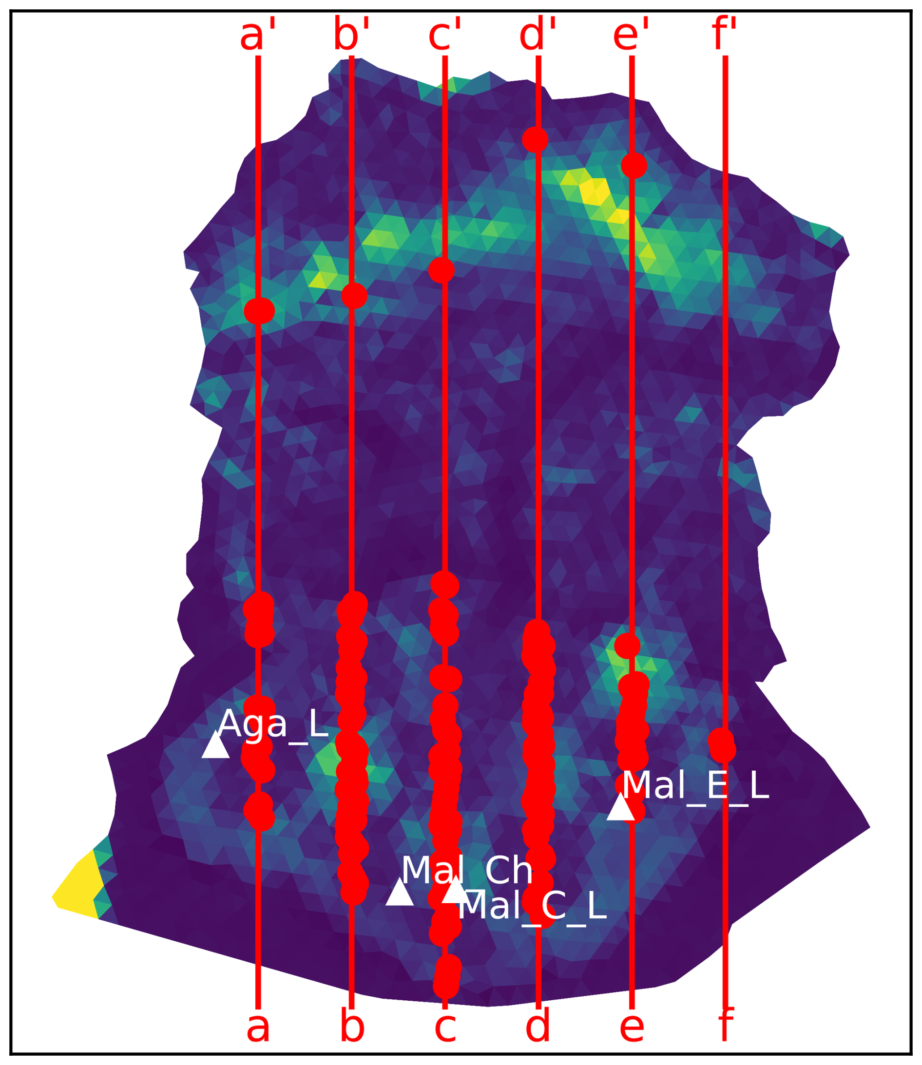
Figure G1 Map of posterior standard deviation of the bed elevation when bed data are held out in a “checkerboard” pattern. Overlain red lines are transects over which we plot the inferred bed using both the full and restricted model. Red points are radar observations that lie within 1 km of transects. White-labeled triangles indicate the location of ablation measurements over summer of 2021.

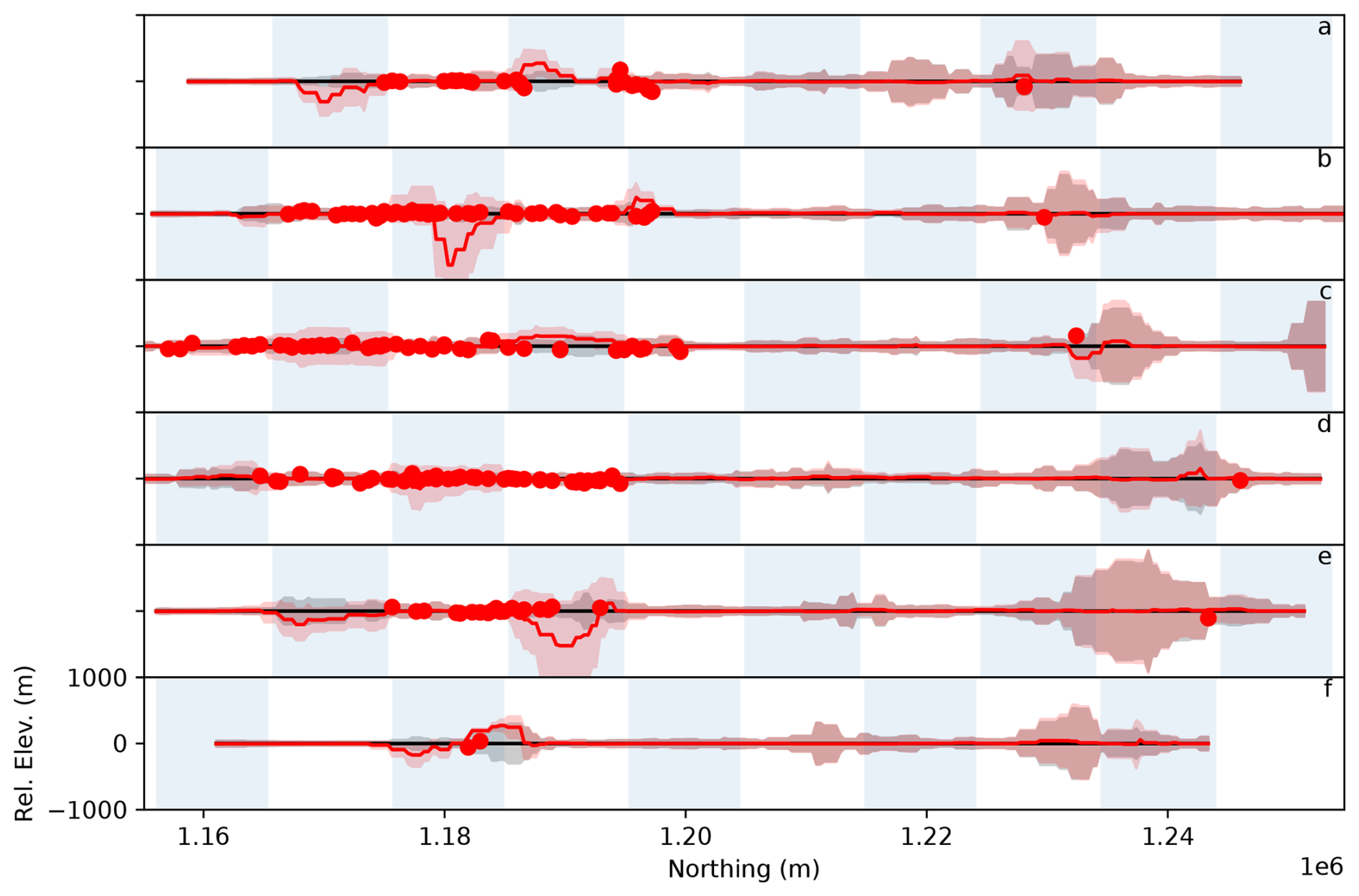
Figure G2 Posterior bed estimates along the profiles appearing in Fig. G1. The mean (solid line) and 3σ credible interval (shading) for both the full (black) and restricted (red) model are shown relative to the full model mean. Red dots indicate radar observations that lie within 1 km of the indicated transect. Blue shading implies that the restricted model does not have access to observations lying within.

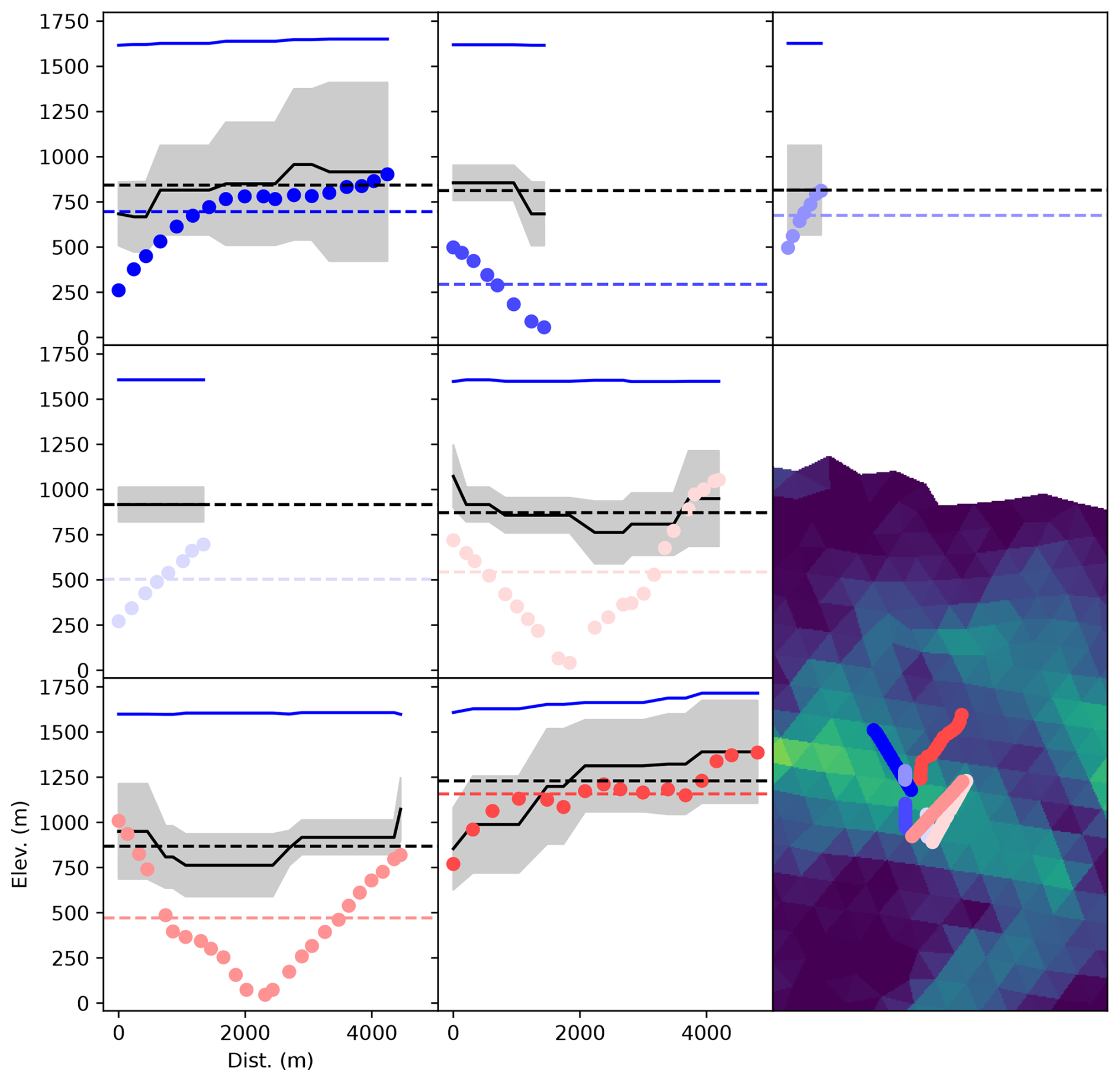
Figure G3 Posterior bed estimates at the color-coded transect locations indicated in the lower right plot (above and to the northwest of the Seward throat). Bed picks appear as colored dots. The surface elevation is given by the thin blue line. The modeled mean (solid line) and 3σ credible interval (shading) are shown in black/gray. Dashed lines indicate modeled and observed means.

Figure G4 Modeled and observed surface mass balance rates for four locations on the Sít' Tlein piedmont lobe indicated in Fig. G1.

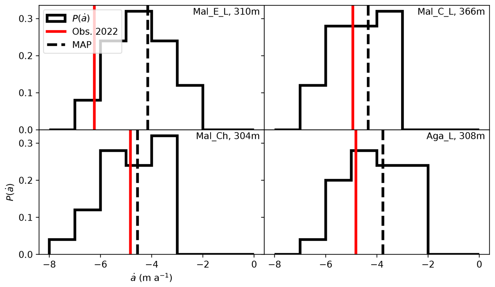
G2 Inferred bed versus a new dataset

During the same field campaign in which we collected the surface mass balance cores described in Fig. 3, we also surveyed a small number of profiles using a ground-based radar system, with bed returns manually picked. These observations were not included in the analysis described in the main text; indeed we did not look at them until after the analysis was complete. The radar-derived bed elevations are plotted alongside (full) model predictions in Fig. G3. We find that in areas that the radar suggests are below 800 m deep, the model and observations exhibit surprisingly good agreement, with the observations falling within the model's posterior 3σ credible interval in most cases. However, the radar returns also suggest the existence of an exceptionally deep V-shaped trough (on the order of 1600 m) that the model does not capture. This disagreement is vexing and points to a physical inconsistency in one of the datasets involved. Because 𝖲𝗉𝖾𝖼𝖤𝖨𝖲 has been verified to conserve mass precisely, the classical glaciological formula of area-integrated mass conservation

$$\begin{array}{}\text{(G1)}& \underset{A}{\int }\dot{a}-{\displaystyle \frac{\partial H}{\partial t}}\mathrm{d}A=\underset{s}{\int }\stackrel{\mathrm{‾}}{\mathit{u}}H\cdot \mathit{n}\mathrm{d}s\end{array}$$

holds, where s is the cross-section, and A is the contributing area. Examining this relation, we observe that there are a few ways in which the model could produce a thickness that is too low. First, the surface mass balance could be underestimated. While three separate field campaigns spanning 70 years (Sharp, 1951; Marcus and Ragle, 1970; and the present work) have established approximate accumulation and net balance rates that are consistent with the model, these observations also cannot account for potential internal accumulation, which could be a source of discrepancy – although it is difficult conceptualize a means for meltwater to refreeze in the relatively temperate climate of coastal Alaska. Second, the thinning rate (which the model successfully reproduces) could be underestimated. Although we expect the laser altimetry from which it is derived here to be accurate, and the time differences between measurements are long, there are also potential confounding factors – such as changes in firn compaction rates – that may introduce bias. Third, the ITS_LIVE-based surface velocity observations (which, again, 𝖲𝗉𝖾𝖼𝖤𝖨𝖲 successfully reproduces) could be overestimated or might not represent the true temporal average which is required here. Indeed, a reproduction of the inference described in the main text with the additional radar-derived measurements described here can reproduce said measurements – at the cost of locally underestimating surface velocities relative to observations. We believe that this is the most likely scenario and hope to perform a more detailed analysis in future work. Finally, it is possible that the radar observations themselves are mistaken. It is notably difficult to obtain high-quality bed returns in extreme topography due to both clutter from off-nadir returns and the attenuation of signals in thick, temperate ice, which is why the IceBridge dataset contains no observations for this location to begin with.

While the disagreement described above remains a mystery, it seems to be relatively localized, and we do not expect this misfit to materially alter the conclusions of this paper, particularly since the area undergoing the greatest change – the piedmont lobe – is extremely well constrained.

G3 Inferred ablation rates versus partial observations

During the summer of 2021, we collected melt measurements between 4 June and 31 August at four locations at approximately 300 m on the Sít' Tlein lobe (shown in Fig. G1), capturing the majority of the melt season – although these measurements are likely to be an underestimate of the true melt. The posterior distribution of model predictions is shown alongside these observations in Fig. G4. While the model's predicted mass balance is quite uncertain (because we allow for annual noise in the prediction), the magnitude of the melt is in reasonable agreement with observations. It is worth noting that we did not explicitly impose any constraints on the surface mass balance below the ELA in this analysis; the recovery of rates that are reasonable with respect to observations occurs solely because such rates are required to reproduce the observed geometry and its rate of change.