Temporal stability of a new 40-year daily AVHRR land surface temperature dataset for the pan-Arctic region

Land surface temperature (LST) has gained increased attention in cryospheric research. While various global satellite LST products are available, none of them is specially designed for the pan-Arctic region. Based on the recently published EUMETSAT Advanced Very High Resolution Radiometer (AVHRR) fundamental data record (FDR), a new LST product (1981–2021) with daily resolution is developed for the pan-Arctic region. Validation shows good accuracy with an average mean absolute error (MAE) of 1.71 K and a MAE range of 0.62–3.07 K against in situ LST data from the Surface Radiation Budget (SURFRAD) network and Karlsruhe Institute of Technology (KIT) sites. Long-term stability, a strong requirement for trend analysis, is assessed by comparing LST with air temperatures from ERA5-Land (T2M) and air temperature data from the EUSTACE (https://www.eustaceproject.org, last access: 17 December 2024) global station dataset. Long-term stability might not be fulfilled mainly due to the orbit drift of the NOAA satellites. Therefore, the analysis is split into two periods: the arctic winter months, which are unaffected by solar illumination and, therefore, orbital drift, and the summer months. The analysis for the winter months results in correlation values (r) of 0.44–0.83, whereas for the summer months (r) values range between 0.37–0.84. Analysis of anomaly differences revealed instabilities for the summer months at a few stations. The same stability analysis for the winter months revealed only one station with instabilities in comparison to station air temperature. Discrepancies between the temperature anomalies recorded at the stations and ERA5-Land T2M were also found. This highlights the limited influence of orbital drift on the LST product, with the winter months presenting good stability across all stations, which makes these data a valuable source for studying LST changes in the pan-Arctic region over the last 40 years. This study concludes by presenting LST trend maps (1981–2021) for the entire region, revealing distinct warming and cooling patterns.

1 Introduction

In recent decades, the warming in the Arctic has been much faster than in the rest of the world. Studies (Chylek et al., 2022; Rantanen et al., 2022) indicate a warming up to 4 times faster since 1979. This phenomenon, known as Arctic amplification, is visible in both instrumental records and model simulation (Dada et al., 2022). The Arctic Monitoring & Assessment Programme (AMAP) highlights diminishingly long cold spells and increasingly high extreme temperatures, leading to rapid changes in the cryosphere (Arctic Monitoring and Assessment Programme (AMAP), 2021). These episodes affect the sensitive Arctic ecosystem; vegetation dynamics; large-scale circulation patterns; and the distribution of snow, ice and permafrost (Maturilli et al., 2019). Permafrost, a crucial component of arctic ecosystems, is particularly sensitive to increasing air temperatures and changes in the snow regime. Thawing permafrost affects the stability of the bedrock, damages infrastructures, and releases massive quantities of organic carbon (Christensen et al., 2004; Miner et al., 2022). These potential threats highlight the importance of monitoring climate variables such as temperature in the arctic regions (Hachem et al., 2012; Urban et al., 2013). Rapid changes in land surface temperature (LST) patterns have been observed in the Arctic region (Reiners et al., 2021). LST can be used as an indicator of the thermal state of the ground and has, in the last decade, been increasingly used in arctic research and permafrost modelling (Westermann et al., 2009; Obu et al., 2019; Batbaatar et al., 2020; Nielsen-Englyst et al., 2021). LST observations are available from in situ stations or climate models. However, these sources are insufficient to spatially resolve land surface characteristics and their response to climate change at a hemispheric scale (Nitze et al., 2018; Bartsch et al., 2023).

In contrast, satellite data can derive spatially comprehensive information on LST dynamics (Li et al., 2013, 2023b). LST is mainly derived from thermal infrared (TIR) radiation measured by satellites with algorithms based on radiative transfer (RT) equations (Li et al., 2013). Passive microwave (MW) measurements are another source of LST data. MW measurements are less affected by clouds than TIR data, but emissivity is challenging to derive for these wavelengths, especially over snow-covered ground (Jiménez et al., 2017; Ermida et al., 2017). LST is a critical parameter in Earth’s surface and water energy balance and is widely exploited across different research fields: cryosphere, geology, vegetation monitoring, hydrology, and urban management (Li et al., 2013; Guillevic et al., 2018). From a climate perspective, LST is needed to evaluate land surface and land–atmosphere exchange processes, constrain surface energy budgets and model parameters, and provide observations of surface temperature change globally and in key regions (Guillevic et al., 2018). LST is defined as an essential climate variable (ECV) by the Global Climate Observing System (GCOS). To retrieve statistically significant changes in ECVs, a time series of at least 30 years is needed (WMO, 2010). Typical LST products include the Pathfinder, GLASS, MODIS, ASTER, and Landsat products (Good et al., 2022; Reiners et al., 2023; Li et al., 2023a), as well as the Spinning Enhanced Visible and Infrared Imager (SEVIRI) LST product produced within the framework of the European Organisation for the Exploitation of Meteorological Satellites (EUMETSAT) Satellite Application Facility on Land Surface Analysis (LSA-SAF) (Freitas et al., 2010; Trigo et al., 2011).

Although many satellite LST datasets with different temporal and spatial resolutions exist, only the Advanced Very High Resolution Radiometer (AVHRR) on board the NOAA and MetOp satellites series covers over 4 decades. EUMETSAT published a new AVHRR fundamental data record (FDR) in May 2023 (https://navigator.eumetsat.int/product/EO:EUM:DAT:0862, last access: 17 December 2024). This dataset was homogeneously produced and consists of reflectance and brightness temperatures covering 1978–2021. It is based on reprocessed near-real-time (NRT) observations from 17 AVHRR instruments on board NOAA satellites TIROS-N to NOAA-19, as well as EUMETSAT satellites MetOp-A, MetOp-B, and MetOp-C (EUMETSAT, 2023a). The dataset is provided in the Global Area Coverage (GAC) resolution. Quality control of AVHRR GAC radiances and updates in the retrieval methods offer more accurate results and better uncertainty estimates (Karlsson et al., 2023b). Notably, CLARA-A3, the third edition of the existing cloud albedo and radiation (CLARA) data record, was produced from this FDR (Karlsson et al., 2023a).

Previous LST datasets exist that have a global coverage (Ma et al., 2020; Li et al., 2023b) or were developed for continental (Reiners et al., 2021) or local usage. However, none of them were specifically derived for the pan-Arctic region. The GLASS product, for example, presents data gaps above 45° latitude due to its LST retrieval process that relies on visible channels, which are not available during polar night. Furthermore, the performance of the LST algorithms is strongly tied to the sampling of atmospheric profiles and surface properties used to calibrate the RT models. Different methodologies and data sources have been used in the past, but most LST products rely (entirely or partially) on the SeeBor database, which is built from the Thermodynamic Initial Guess Retrieval (TIGR)-3 database, ERA-40, and radiosonde datasets (Borbas et al., 2005). Taking advantage of the most recent ECMWF version-5 reanalysis (ERA5), Ermida and Trigo (2022) developed a new clear-sky database for the development of LST algorithms. The synthetic database is constructed from ERA5 data chosen with a dissimilarity criterion to ensure a uniform distribution of atmospheric conditions. The clear-sky database shows a significantly wider range of conditions and thus a wider range of brightness temperatures than in the SeeBor database specifically. The pan-Arctic region shows a wide range of temperatures and conditions that are not necessarily common, so it is particularly important to base the RT modelling on a robust and representative database for that region. A new daily LST dataset, presented here for the northern high latitudes (>50° N), is produced based on the EUMETSAT FDR and the clear-sky database (Ermida and Trigo, 2022).

The new LST dataset represents a valuable source for studying LST dynamics and its impacts on regional climates surface energy balance (Hall et al., 2012; Key et al., 2016), vegetation phenology (Li et al., 2021), and temperature hot spots (Mildrexler et al., 2018) and characterizing land use/land cover dynamics. However, to perform climatological analyses, it is crucial that the satellite LST observations are stable and robust (Waring et al., 2023).

The objectives of this paper are first the description of the LST retrieval and validation methods and, second, the assessment of the stability of the new pan-Arctic LST dataset. Relationships and trends with respect to the following datasets are compared: (i) in situ air temperature (Tair) measurements provided by the EUSTACE database and (ii) 2 m air temperature (T2M) data from ERA5-Land for the overlapping period (1981–2020). The comparisons are made for selected sites in the pan-Arctic region. The presence of trends in T2M is well established and is considered one of the major indicators of anthropogenic climate change (IPCC, 2021). Previous studies (Mildrexler et al., 2011; Hachem et al., 2012; Urban et al., 2013; Good et al., 2022) obtained a good correlation between LST and T2M/Tair, although these parameters have different physical meanings and are measured or modelled with different procedures. Hachem et al. (2012) found that LST derived from MODIS and daily near-surface air temperatures are comparable. Good (2016) noted that LST and T2M are very similar when solar heating is low or absent. The NOAA satellites do not have a stable orbit (Ignatov et al., 2004; Latifovic et al., 2012), meaning that over the course of their operating years, their Equator crossing time is shifting (Price, 1984). In the case of LST, drifting orbits could lead to artificial trends in long-term records if only one platform is considered. In the present case, the LST from the different platforms is combined (morning and afternoon overpasses), and the final product is generated over multiple satellites. However, this also means that observed trends are more complex to interpret (Lieberherr and Wunderle, 2018). Orbital drift has a more substantial impact in the Southern Hemisphere and on bare soil (Sobrino et al., 2002; Gleason et al., 2002) than in the Northern Hemisphere. For example, this effect has been neglected in previous studies focusing on the Arctic region (Urban et al., 2013) or lakes (Riffler et al., 2015).

In this study, the analysis is carried out for two cases: (a) polar winter, defined here as December and January, and (b) polar summer, defined here as June and July. Incident solar radiation is zero during polar winter (Lund et al., 2017; Wang and Zeng, 2014); therefore, it is expected that a trend analysis for case (a) should not be affected by orbital drift. This paper is structured as follows: the data used to produce the LST are presented in Sect. 2, and the methodology is described in Sect. 3. Validation results for the LST product are presented in Sect. 4.1. Comparisons with air temperature datasets and trend analysis are presented in Sect. 4.2, 4.3, and 4.4. Finally, discussions and conclusions are presented in Sects. 5 and 6.

2 Data

This study uses the newly generated EUMETSAT AVHRR FDR satellite dataset, one reanalysis dataset, and several weather station datasets. Snow cover information is based on the snow water equivalent (SWE) dataset and snow cover fraction (SCF) from the ESA CCI Snow project.

2.1 EUMETSAT AVHRR FDR

The FDR contains AVHRR reflectance and brightness temperatures for each available orbit and channel. The daily AVHRR data from one satellite provide nearly complete coverage of the globe. AVHRR GAC measurements have been processed using pygac – a Python software package to read and transform AVHRR data in GAC format (https://pygac.readthedocs.io/en/latest/#, last access: 17 December 2024) – including the conversion from counts to reflectance or brightness temperature and cross-calibration of the visible channels of the AVHRR sensor. The two thermal channels are calibrated following the platinum resistance thermometer (PRT), space, and internal calibration target (ICT) count procedure (Kidwell, 1995; Walton et al., 1998). Detailed information is available in PyGAC FDR ATBD (EUMETSAT, 2023b). The data are accompanied by additional metadata (such as orbit overlap and Equator crossing time) and basic quality indicators (EUMETSAT, 2023c). Only satellites carrying the newer versions (AVHRR/2 and AVHRR/3) of the AVHRR are considered in this study. The second version (AVHRR/2) has five spectral channels, and the third version (AVHRR/3) has six but transmits only the data from five channels. Brightness temperature channel 4 is centred at 10.8 µm and brightness temperature channel 5 at 12 µm. The IR calibration procedure is satellite-specific, with no cross-calibration between satellites for IR channels (EUMETSAT, 2023d). The PyGAC AVHRR FDR from EUMETSAT (2023) is available in the Network Common Data Form (NetCDF) format and covers the entire globe (−180, 90, 180, −90°). For each satellite, the orbit files are composited by choosing for each pixel only the observation closest to nadir. The composited files have a spatial resolution of 0.05° × 0.05° pixel size and are available for each satellite twice a day (at daytime and nighttime). This study focuses on the pan-Arctic region. Therefore, only data above 50° N have been processed.

2.1.1 Cloud mask

Cloud cover information is obtained from the CM SAF CLARA-A3 dataset (Karlsson et al., 2023b), which is also based on EUMETSAT AVHRR FDR (EUMETSAT, 2023a). The probabilistic cloud mask (CMAPROB), included in the level-2b product, and quality flags are used. Cloud probabilities range from 0 % to 100 % (EUMETSAT Satellite Application Facility on Climate Monitoring (CM SAF), 2023). The cloud probabilistic detection is based on the naïve Bayesian theory and offers substantial improvement to previous CLARA-A2 data records (Devasthale and Karlsson, 2023).

2.1.2 Snow cover data

Snow cover fraction (SCF) from optical satellite data and snow water equivalent (SWE) products from passive microwave satellite data from the ESA CCI Snow project (https://climate.esa.int/en/projects/snow/, last access: 17 December 2024) are used to obtain information on snow extent (Luojus et al., 2022; Xiao et al., 2024). The SCF “viewable snow” (SCFV) product is derived from the EUMETSAT AVHRR FDR and applied for this study. A value equal to zero means that the pixel is snow-free, and 100 means that the pixel is fully covered by snow. The SWE variable is indicated in millimetres. Both snow products are combined to get a snow mask independent of the availability of the visible channels during polar night.

2.2 ERA5-Land 2 m air temperature

ERA5-Land (Muñoz Sabater et al., 2021), provided by the European Centre for Medium-Range Weather Forecasts (ECMWF), is a downscaled version of the land component of the global ERA5 reanalysis. Compared to ERA5, ERA5-Land shows better stability but reduced accuracy (Urraca and Gobron, 2023). However, the accuracy suffices to capture inter-annual variations (Rantanen et al., 2023). Data from the ERA5-Land monthly averaged air temperature 2 m above the surface are compared to the LST dataset.

2.3 In situ 2 m air temperature

In situ air temperature observations from the EU Surface Temperature for All Corners of Earth (EUSTACE) land station dataset (Brugnara et al., 2019; Rantanen et al., 2023) are used for comparison. This database stores daily minimum (T_min) and maximum (T_max) temperature values recorded at weather stations ∼2 m above the surface. The station dataset has undergone quality controls, was homogenized, and covers the period from 1850 to 2015. Weather stations from the EUSTACE database were selected according to the following criteria:

• The station lies above 50° latitude.

• The underlying ground is composed of permafrost.

• Different latitudes are represented.

• The surrounding area at a station, corresponding to at least 1 GAC pixel, must be homogeneous.

• The time series should cover at least 30 years.

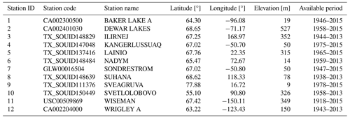
Based on these criteria, 12 stations have been selected (Fig. 1 and Table 1).

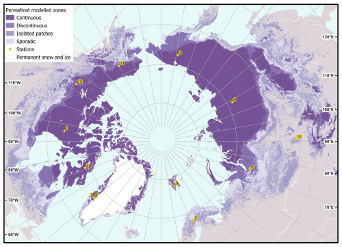
Figure 1 Selected EUSTACE stations with their IDs (Table 1). Permafrost zonation map adapted from Obu et al. (2018).

Table 1 Selected EUSTACE meteorological stations with WMO code, geolocation, elevation. and available period.

2.4 Auxiliary data

The generation of LST data requires auxiliary datasets:

• Skin temperature (T_skin) and total column water vapour (TCWV) from the MERRA-2 reanalysis dataset (M2T1NXSLV, variables are labelled TS and TQV) are used. The data come at hourly temporal resolution with a spatial resolution of 0.5° × 0.625°. Nearest neighbour resampling was performed to match the AVHRR spatial resolution and scanline time, i.e. as in the work of Ma et al. (2020). MERRA-2 is preferred over other reanalysis products with finer spatial resolution to allow comparison with the GLASS product (Ma et al., 2020) and to keep the LST retrieval independent of ERA5-Land, which will be used for the stability analysis.

• ESA CCI Land Cover 1992–2015 and Copernicus ICDR Land Cover 2016–2020 datasets are used. Both datasets are consistent with each other. Their spatial resolution was decreased to match AVHRR GAC spatial resolution. The class labels follow the Land Cover Classification System (LCCS) developed by the United Nations (UN) Food and Agriculture Organization (FAO) (Copernicus Climate Change Service, Climate Data Store, 2019).

• Atmospheric profiles from the Clear-Sky Database developed at LSA-SAF (Ermida and Trigo, 2022) are used for the RT modelling (RTM). This database contains atmospheric profiles such as temperature, specific humidity, and ozone on 137 model levels (full vertical resolution), sampled from ERA5 for the 2009–2019 period. The sampling technique follows the method of Chevallier et al. (2000). Surface variables like T2M, surface pressure, T_skin, and emissivity are obtained from the combination of ERA5 and satellite data to ensure the best possible representation of the surface conditions. Column variables, such as TCWV and total cloud cover (TCC), are also present in the database. The atmospheric profiles are classified on TCWV varying from 0 to 60 mm and TS ranging from 190 to 340 K.

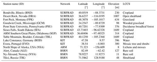
• In situ LST measurements from the Surface Radiation Budget (SURFRAD) network, the Karlsruhe Institute of Technology (KIT) network (Göttsche et al., 2016; Martin et al., 2019), the Atmospheric Radiation Measurement Climate Research Facility US Department of Energy (ARM) site at the North Slope of Alaska (NSA), and radiation data from the Baseline Surface Radiation Network (BSRN) (Maturilli, 2020; Cox and Halliwell, 2021; Kustov, 2018, 2023) are used for validation. Table 2 lists the stations. The KIT stations, which are part of LSA SAF's validation effort and supported by EUMETSAT, are located in different climate zones (Göttsche et al., 2016). In situ LST is computed from their radiation components as in Martin et al. (2019). The broadband emissivity (BBE) is obtained from channel effective emissivity data provided in the ASTER GED (Hulley et al., 2015) with the linear equation described in Cheng et al. (2013).

• The Copernicus digital elevation model (DEM) GLO-90 upscaled to 0.05° spatial resolution is used (https://doi.org/10.5270/ESA-c5d3d65, Copernicus digital elevation model (DEM) GLO-90, 2024) for the RT modelling. This dataset represents the surface of the Earth and is based on radar satellite data obtained from the TanDem-X Mission.

Table 2 Description of the stations used for LST validation. Station name and ID, the network the station belongs to, latitude, longitude, elevation, and the dominant land cover type are listed.

3 Methods

LST can be retrieved from thermal infrared data with the well-established split-window (SW) method (Ma et al., 2020; Yang et al., 2020; Reiners et al., 2021). Since 1983 (Price, 1984; Prata, 1994) different algorithms have been developed to obtain LST as a function of the satellite-recorded brightness temperature (BT). The split-window approach takes advantage of the different water vapour absorption characteristics of two adjacent channels (Lieberherr et al., 2017; Ma et al., 2020). LST is affected by many factors, which requires additional terms to model the effects of land cover type, viewing angle, and topography (Trigo et al., 2017).

3.1 Generalized split-window algorithm

For this study the generalized split-window (GSW) algorithm, developed by Wan and Dozier (1996) (Eq. 1) and used within the framework of LSA-SAF (Trigo et al., 2008b; Ermida and Trigo, 2022), is selected. The GSW performs well on a global scale and has the highest relative accuracy among a selection of SW algorithms investigated in the work of Yang et al. (2020). The GSW depends on channel-effective emissivity and sensor-specific coefficients that must be determined for the expected atmospheric and surface conditions.

$$\begin{array}{}\text{(1)}& \begin{array}{rl}{T}_{\mathrm{s}}& =\left(A_{\mathrm{1}}+A_{\mathrm{2}}{\displaystyle \frac{\mathrm{1}-\mathit{ϵ}}{\mathit{ϵ}}}+A_{\mathrm{3}}{\displaystyle \frac{\mathrm{\Delta }\mathit{ϵ}}{{\mathit{ϵ}}^{\mathrm{2}}}}\right)(T_{\mathrm{11}}+T_{\mathrm{12}})\\ & +\left(B_{\mathrm{1}}+B_{\mathrm{2}}{\displaystyle \frac{\mathrm{1}-\mathit{ϵ}}{\mathit{ϵ}}}+B_{\mathrm{3}}{\displaystyle \frac{\mathrm{\Delta }\mathit{ϵ}}{{\mathit{ϵ}}^{\mathrm{2}}}}\right)(T_{\mathrm{11}}-T_{\mathrm{12}})+C,\end{array}\end{array}$$

where T₁₁ and T₁₂ denote BT of channels centred at approximately 11 and 12 µm; $\mathit{ϵ}=({\mathit{ϵ}}_{\mathrm{11}}+{\mathit{ϵ}}_{\mathrm{12}})/\mathrm{2}$; $\mathrm{\Delta }\mathit{ϵ}=({\mathit{ϵ}}_{\mathrm{11}}-{\mathit{ϵ}}_{\mathrm{12}})$; and A_i, B_i, and C are split-window coefficients (SWCs).

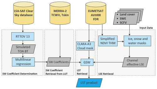
Figure 2 LST retrieval from AVHRR data. Input data are shown at the top. The leftmost box refers to the SW coefficient determination; the next box on the right displays the look-up-table storing coefficients for different atmospheric and surface conditions. The second box from the right presents the cloud mask application to the thermal channels and the rightmost panel the process of generating land surface emissivity (LSE) based on land cover and NDVI information.

The split-window coefficients in Eq. (1) are obtained by applying multi-linear regression on a set of simulated BTs against a calibration database. Simulated BTs are obtained by performing RTM with version 13 of the Radiative Transfer for TOVS (RTTOV) developed at NWC SAF (Saunders et al., 2018). The Python wrapper was used in this study (Hocking et al., 2021). Atmospheric profiles and surface and column variables from the clear-sky profile database developed by Ermida and Trigo (2022), complemented by elevation information and satellite viewing angles, are ingested by RTTOV. The clear-sky profile database contains 97 files, each file containing approximately 1000 atmospheric profiles corresponding to a different class of TCWV and T_skin. In total, the database contains 82 793 profiles, and each profile possesses 6 different TS values and 25 pairs of emissivity at 11 and 12 µm. More details can be found in Ermida and Trigo (2022). Convolving the top-of-atmosphere radiances produced by RTTOV with the specific AVHRR response functions yields BTs as seen by the different sensors for different atmospheric and viewing conditions. RT modelling was performed on the calibration dataset for each satellite and 15 different satellite view zenith angles (VZAs) ranging from 0 to 70°. Table 3 summarizes the construction of the simulation dataset. Finally, the calibration was performed independently for each class, and for each class, the samples were split into a training (70 %) and test (30 %) set, and multilinear regression was performed on the resulting BTs. Based on the test sets, look-up tables (LUTs) with coefficients are created for each satellite. The LUTs are organized into classes of TCWV and T_skin, allowing the allocation of the right SWC to the encountered atmospheric conditions. Mean absolute error (MAE), the coefficient of determination (R²), and root mean square error (RMSE) are computed for all coefficients to keep track of the general performance of the RTM.

(Ermida and Trigo, 2022)

Table 3 Summary of the simulation dataset: the number of profiles used and the number of instances of view zenith angles (VZAs), TS, and LSE are shown.

3.1.1 Land surface emissivity retrieval

Land surface emissivity (LSE) is retrieved by combining the simplified normalized difference vegetation index (NDVI) threshold method (SNDVI_THM) (Sobrino et al., 2008) based on Sobrino and Raissouni (2000) with channel emissivity data from spectral libraries and static land cover classifications.

First, 10 d NDVI maximum value composites (MVCs) are generated from the AVHRR channels 1 and 2. NDVI thresholds that determine whether a pixel is considered fully vegetated or entirely bare soil are set. In the present case, NDVI_soil is set to 0.2, and NDVI_veg is set to 0.5 (Sobrino et al., 2001). All pixels that have 0.2 < NDVI < 0.5 are considered mixed pixels, and the corresponding emissivity is obtained by using the proportion of vegetation (P_v) method (Sobrino et al., 2008) (Eq. 2) that weighs the emissivity of bare soil (ϵ_si) and vegetation (ϵ_vi) for AVHRR channel i (i=4 or 5).

$$\begin{array}{}\text{(2)}& {\mathit{ϵ}}_i={\mathit{ϵ}}_{\mathrm{v}i}{P}_{\mathrm{v}}+{\mathit{ϵ}}_{\mathrm{s}i}(\mathrm{1}-P_{\mathrm{v}})\end{array}$$

ϵ_si and ϵ_vi are taken from a LUT based on information from spectral libraries (Trigo et al., 2008a; Peres and DaCamara, 2005). The emissivity of pixels with NDVI <0.2 or NDVI >0.5 is set to ϵ_si and ϵ_vi respectively. Here, the channel emissivities from Trigo et al. (2008b) (Table I) are used. The IGBP classes (Sulla-Menashe and Friedl, 2018) are converted to land cover classes of the ESA CCI project with plant functional type look-up tables (Wang et al., 2023). From 1992 to 2020, the ESA CCI land cover at the 12 selected stations changed very little. Therefore, to reduce emissivity uncertainties due to unknown land cover information before 1992, a static land cover from 2000 is used throughout the project (Freitas et al., 2010). The land cover was previously upscaled to the resolution of the AVHRR dataset. P_v is obtained from NDVI with Eq. (3) (Carlson and Ripley, 1997).

$$\begin{array}{}\text{(3)}& P_{\mathrm{v}}={\left({\displaystyle \frac{\text{NDVI}-{\mathrm{NDVI}}_{\mathrm{soil}}}{{\mathrm{NDVI}}_{\mathrm{veg}}-{\mathrm{NDVI}}_{\mathrm{soil}}}}\right)}^{\mathrm{2}}\end{array}$$

Pixels with low NDVI values (NDVI <0.2) are defined as bare soil. Such NDVI values can also indicate the presence of snow or cloud cover. Snow cover extent information is retrieved from two data products from the ESA CCI Snow project, and cloudy pixels are masked out in the final LST product. A threshold of 70 % of SCFV or 4 mm for SWE is used to categorize the pixel as fully snow-covered. Snow-covered pixels are assigned to laboratory emissivity spectra values of medium snow (Fig. 5 of Hulley et al., 2014). Water pixels and permanent snow and ice areas are retrieved based on land cover information from the ESA land cover CCI for the year 2000 and are assigned to channel effective emissivity values from Hulley et al. (2014).

3.2 LST retrieval

LST is retrieved as follows: (i) all necessary data (BTs, cloud mask, emissivity, and atmospheric data) are read; (ii) atmospheric data from MERRA-2 (TS and TQV) are downscaled to GAC spatial resolution, and the corresponding timestamp is matched with the scanline time for each pixel; (iii) based on satellite identification number, satellite viewing angle, total column water vapour (TQV), skin temperature (TS), and the corresponding SWC from the LUT are assigned to each pixel; and (iv) LST is computed from channel BTs, emissivities, and the assigned SWC (Eq. 1). Pixels with a satellite view zenith angle greater than 40° and the MAE of the test set in the RTM simulations greater than 0.5 K are masked out.

3.3 Validation procedure

The AVHRR LST dataset is validated against in situ data from different sites (Table 2). In situ LST and AVHRR LST datasets are jointly based on acquisition time and geolocation. The closest pixel to the station is taken, and a time difference of up to 5 min between the satellite overpass and the in situ measurement is considered. For Lake Constance, a time difference of up to 30 min is allowed. Similarly, as in Ma et al. (2020), 3σ filtering was performed to remove outliers (Pearson, 2002). The most accurate surface temperatures can be obtained over large water bodies, such as lakes and reservoirs. Densely vegetated surfaces are also particularly suitable for LST validation (Coll et al., 2009).

3.4 LST AVHRR time series generation

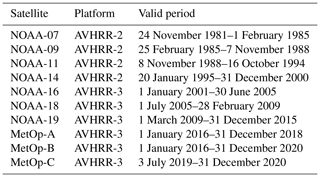
Depending on the heterogeneity of the land cover, between 4 and 9 AVHRR LST GAC pixels are extracted around each station (Table 1). Pixels that have a cloud probability higher than 0.1 are removed, and the average of the remaining pixels is computed. Pixels with a cloud probability of 0.1 or lower are considered cloud-free (Karlsson et al., 2023b). This cloud probability threshold is a compromise between data availability and avoiding cloud contamination. Daytime data from NOAA-7, NOAA-9, NOAA-11, NOAA-14, NOAA-16, NOAA-18, and NOAA-19 (satellites with ascending (northbound) Equator crossing times), as well as the entire MetOp series (satellites with descending (southbound) Equator crossing times), are considered for constructing the time series. The considered period for each satellite is chosen to minimize orbital drift and avoid the outage periods (EUMETSAT, 2023d). The retained periods are listed in Table 4.

Table 4 Considered time period for each satellite and sensor that it carries.

Once the relevant periods are extracted, outlier detection is performed based on a 10 d rolling window analysis, and detected outliers are removed. Daily temperature variability is very high (Mildrexler et al., 2011), and AVHRR-derived LST time series are subject to noise. Therefore, monthly means are computed from concatenated daytime time series for further analysis.

3.5 Time series analysis

The AVHRR LST monthly means time series is compared with two independent datasets: ERA5-Land and EUSTACE Tair. ERA5-Land pixels collocated to each weather station are selected, and values of T2M for the same position are extracted. The EUSTACE Tair data are filtered to keep only data that passed all quality assurance checks (Menne et al., 2012), and monthly means are computed. This yields time series of LST, ERA5-Land T2M (hereafter referred to as “T2M”), and EUSTACE Tair (hereafter referred to as “Tair”) for each station. Before performing the actual stability analysis and starting with trend analysis, the overall relationship between the datasets is assessed by computing statistical parameters such as the Pearson correlation coefficient (r), the MAE, and the RMSE. Previous studies (Mildrexler et al., 2011; Hachem et al., 2012; Westermann et al., 2012; Urban et al., 2013) found variability in the LST–Tair correlation depending on the season and the land cover.

Then, anomalies of the monthly mean time series are computed for the LST, T2M, and Tair time series at all stations to remove the strong seasonal cycle inherent to temperature data (Good et al., 2022). A temperature anomaly describes the difference from a baseline climatology. In the present study, the anomalies are computed by subtracting the mean temperature for the entire time series from the monthly values. The LST, T2M, and Tair anomalies are compared by computing the Pearson correlation coefficient (r). Three different periods are considered for the anomaly analysis: (a) the entire year, (b) polar winter (December, January), and (c) polar summer (June and July). June and July are chosen as summer months to respect the symmetry of the winter period. First, the relationship between the anomalies of the different datasets is evaluated with the Pearson correlation coefficient (r), and the general stability of the LST dataset is assessed by computing the trends of the anomaly differences. Three sets of differences are computed:

$$\begin{array}{}\text{(4)}& {\displaystyle }\mathrm{\Delta }{\mathrm{Tanom}}_{\mathrm{LST}-\mathrm{T}\mathrm{2}\mathrm{M}}={\mathrm{LST}}_{\mathrm{anom}}-\mathrm{T}\mathrm{2}{\mathrm{M}}_{\mathrm{anom}}\text{(5)}& {\displaystyle }\mathrm{\Delta }{\mathrm{Tanom}}_{\mathrm{LST}-\mathrm{Tair}}={\mathrm{LST}}_{\mathrm{anom}}-{\mathrm{Tair}}_{\mathrm{anom}}\text{(6)}& {\displaystyle }\mathrm{\Delta }{\mathrm{Tanom}}_{\mathrm{Tair}-\mathrm{T}\mathrm{2}\mathrm{M}}={\mathrm{Tair}}_{\mathrm{anom}}-\mathrm{T}\mathrm{2}{\mathrm{M}}_{\mathrm{anom}},\end{array}$$

where LST_anom denotes the LST anomalies, and T2M_anom and Tair_anom represent the ERA5-Land air temperature anomalies and EUSTACE air temperature anomalies respectively. The anomaly differences are represented by ΔTanom. The stability analysis is performed separately on the summer and winter periods. Non-parametric trend analysis is performed on the anomaly differences using the Theil–Sen slope to quantify the trend and the Mann–Kendall test to determine its significance. The Python implementation of the Mann–Kendall trend test (Hussain and Mahmud, 2019) was used in this work. Finally, trends are computed at each station for the entire year for all three datasets, and summer and winter trends are computed for the whole pan-Arctic region.

4 Results

In the first parts of the Results section (Sect. 4.1.1 and 4.1.2), the performances of the GSW algorithm and the validation results are presented. The remaining subsections present the relationships of the different datasets as well as the stability analysis and trend computation.

4.1 LST validation results

4.1.1 Performance of the split-window algorithm

Multi-linear regression was used to fit Eq. (1) to the RTM results for each class of TCWV and T_skin in a training set that consisted of 70 % of the samples, thereby retrieving the corresponding SWCs. The performance of the regression model was evaluated with the remaining independent samples (test set). The performance of the model is assessed by using the MAE and the coefficient of determination (R²). The values shown in Fig. 3 are mean values across all satellites: the MAEs of the predictions are below 0.5 K for dry conditions (TCWV <30) and low satellite viewing angle (VZA <40). In cases with very moist atmospheres and high VZA (VZA >50), the MAE increases substantially, and R² is considerably lower (R²<0.92). Higher temperatures and higher VZA also lead to an increased error. The overall MAE is always below 2 K for water vapour below 50 mm TCWV. MAE values above 2 K are reached for high TCWV (TCWV >50 mm) and high VZA values (VZA >50°). Overall, the amount of water vapour in the Arctic atmosphere is low, which indicates that the model is well suited for the present use case.

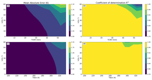
Figure 3 Split-window algorithm (SWA) performances: (a) distribution of the mean absolute error (MAE) and (b) coefficient of determination as a function of the view zenith angle (VZA) and total column water vapour (TCWV). Panels (c) and (d) show the corresponding distributions dependent on VZA and T_skin.

4.1.2 Validation with in situ LST

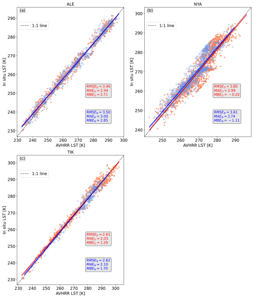
Figures 4 and 5 show the validation results for NOAA-14, NOAA-16, NOAA-17, NOAA-18, and NOAA-19 and MetOp-A, MetOp-B, and MetOp-C against in situ LST from the validation sites in Table 2. The validation is separated for daytime (represented in red) and nighttime (blue). For each validation site, the MAE, RMSE, and mean bias error (MBE) are shown. The match-up with the SURFRAD stations covers the period from 1985 to 2020, the match-up period for the KIT station in EVORA (EVO) starts in 2009 and ends in 2020, the match-up period for Lake Constance starts in 2016 and ends in 2020, and finally the match-up period for the ARM site at the North Slope of Alaska (NSA) starts in 2007 and ends in 2012. Regarding the BSRN data, for the station in Alert (ALE) the match-up period starts in 2004 and ends in 2014, for Ny-Ålesund (NYA) it starts in 2006 and ends in 2020, and for Tiksi (TIK) it starts in 2010 and ends in 2018. EVO is located in an evergreen oak woodland with approximately 33 % tree crown cover, which can affect the satellite-retrieved LST due to directional effects (Rasmussen et al., 2011; Guillevic et al., 2013; Ermida et al., 2014). Due to this anisotropy, the surface in EVO presents high temperature differences between trees and the ground. The nighttime in situ measurements in EVO are therefore more suited than daytime observations. The surface is very heterogeneous at the NSA site, the station being close to lagoons (North Salt Lagoon and Imikpuk Lake) and very close to the coast. This explains why the performances are much worse during summertime than during wintertime when the entire area is snow and ice covered. Similarly, the BSRN stations are all located near the coast. In addition, the terrain around NYA station is mountainous and heterogeneous, leading to worse validation results. The in situ data for Lake Constance (BOD) are collected during the operating hours of the ferry and are thus only available during daytime. Both daytime and nighttime data are considered at the SURFRAD sites. BOD has the fewest available points due to the shorter match-up period. The overall RMSE range for the 10 stations is 0.80–3.43 K. The highest performance is reached at BOD. LSTs are more stable over water bodies, and water emissivity is less prone to inducing significant uncertainties (Masuda et al., 1988; Niclòs et al., 2005). On land, during the daytime, the highest agreement was obtained for the Desert Rock (DRA) and Goodwin Creek (GCM) sites. The lowest agreement was found at Fort Peck (FPK). During nighttime, the highest agreement was obtained at Sioux Falls (SFA), and the worst nighttime agreements were obtained at Desert Rock (DRA) and Fort Peck (FPK). Compared to previous studies on AVHRR LST (Ma et al., 2020; Reiners et al., 2021; Li et al., 2023a), the present dataset shows a similar accuracy and precision.

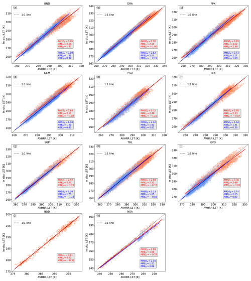
Figure 4 AVHRR LST versus in situ LST at (a) Bondville (BND), (b) Desert Rock (DRA), (c) Fort Peck (FPK), (d) Goodwin Creek (GCM), (e) Penn State University (PSU), (f) Sioux Falls (SFA), (g) Southern Great Plains (SGP), (h) Table Mountain (TBL), (i) Evora (EVO), (j) Lake Constance (BOD), and (k) North Slope of Alaska (NSA). Red represents daytime measurements, and blue represents nighttime measurements. Match-up periods are provided in the text.

Figure 5 AVHRR LST versus in situ LST at BSRN stations: (a) Alert, Lincoln Sea (ALE); (b) Ny-Ålesund, Svalbard (NYA); and (c) Tiksi, Russia (TIK). Red represents the daytime measurements, and blue represents the nighttime measurements. Match-up periods are provided in the text.

4.1.3 Comparison with the GLASS dataset

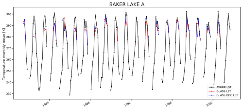
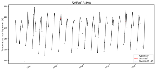
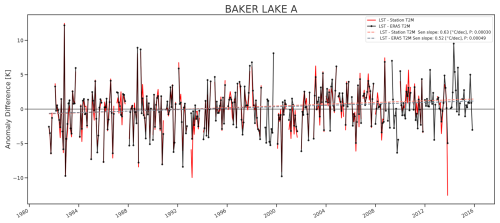
The pan-Arctic AVHRR LST dataset is compared against the well-established GLASS product (Zhou et al., 2019; Ma et al., 2020) that provides twice-daily LST observations for the whole globe for the 1980–2000 period. Figures 6 and 7 present a comparison of monthly means at two stations located in the Arctic (BAKER LAKE A and SVEAGRUVA). The classical GLASS LST, the orbital-drift-corrected (ODC) GLASS LST, and the pan-Arctic AVHRR LST are compared at the pixel closest to the station. In the high northern latitudes, the GLASS product is only available during the summer months. This is particularly visible for the SVEAGRUVA site (located on Svalbard), where very few GLASS observations are available. Also at BAKER LAKE A our product presents considerably more and slightly higher values, which can be explained by the different cloud masking and emissivity computation.

Figure 6 Monthly mean LST product comparisons at BAKER LAKE A.

Figure 7 Monthly mean LST product comparisons at SVEAGRUVA.

4.2 Relationships between the temperature datasets

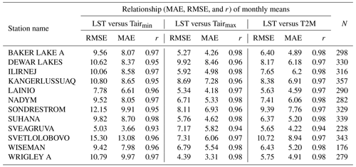
The relationship between AVHRR LST and station EUSTACE Tair and the relationship between AVHRR LST and ERA5-Land T2M at each EUSTACE station are first assessed by computing the Pearson correlation coefficient (r), the MAE, and RMSE of the monthly mean temperature data (see Sect. 3.5). Comparisons against Tair_min show, in general, higher RMSE and MAE values than comparisons against Tair_max and T2M (Table 5). For the stations in Table 5, the mean MAE values are 8.47, 5.56, and 5.92 K for LST versus −Tair_min, −Tair_max, and − T2M respectively. Stations WRIGLEY A, WISEMAN, and SVEAGRUVA exhibit lower MAE and RMSE values than the other stations. WISEMAN and SVEAGRUVA have slightly fewer comparison samples (N<230). SVEAGRUVA, located in Svalbard, is the northernmost station and experiences persistent cloud cover, leading to fewer usable satellite observations. The EUSTACE time series at WISEMAN is shorter due to missing data. WRIGLEY A exhibits low MAE and RMSE values compared to Tair_max but presents similar values to other stations compared to Tair_min.

As to be expected, the analysis reveals a high degree of correlation between monthly LST, Tair, and T2M with correlation coefficients all above 0.9 (r) (Table 5). In line with higher RMSE and MAE, Tair_min has slightly lower (r) values compared to LST. The better performance of Tair_max can be attributed to the closer daytime overpass of the NOAA–MetOp satellites (Good et al., 2022). Conversely, Tair_min is generally recorded during night.

Table 5 MAE, RMSE, and Pearson coefficient (r) at the selected EUSTACE stations for monthly mean comparisons. N is the number of samples.

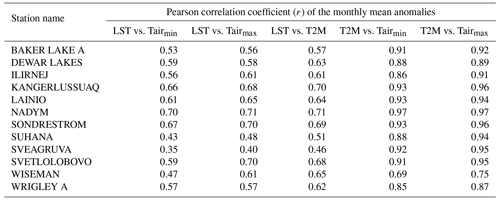
The relationship between the monthly AVHRR LST anomalies versus EUSTACE Tair anomalies and ERA5-Land T2M anomalies is assessed with the Pearson correlation coefficient (r) (Table 6). All stations except SUHANA (Siberia) and SVEAGRUVA (Svalbard) display strong positive correlations (r>0.5) between LST and both air temperature datasets (Tair and T2M). Correlations are consistent for both air temperature datasets; only minor differences are visible. The r values for comparing Tair with T2M are higher than those in the corresponding comparison with LST. Correlations of LST versus T2M anomalies vary between 0.46 (r) and 0.71 (r). For Tair_max versus LST, the r values r of are between 0.40 and 0.71, whereas for Tair_min, r has a range of 0.35–0.70. In general, slightly higher r values are obtained for the comparison against T2M than Tair. Comparison values of Tair versus T2M have values of r between 0.69 and 0.97. Similarly to in Table 5, lower r values are found for the comparison with Tair_min than for Tair_max. The lowest correlation value between T2M and Tair is obtained at WISEMAN (Alaska). NADYM (Russia) shows consistently high correlations (r≈0.7) across all comparisons and has the highest correlation value for the Tair versus T2M evaluation. Previous studies have also found high correlations between station Tair and LST data for other LST datasets (Urban et al., 2013; Good et al., 2022), e.g. from the ESA CCI project (Ghent et al., 2023). The differences in r between Tables 5 and 6 can be attributed to a phase shift between the anomalies and to a strong seasonal signal present in the time series on monthly means.

Table 6 Correlation coefficient (r) from all stations for the comparison between the LST monthly mean anomalies versus the T2M and Tair monthly mean anomalies.

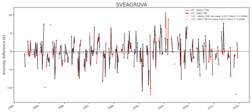
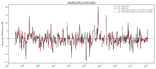
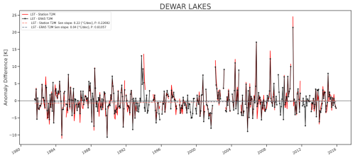
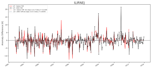
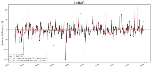
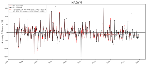
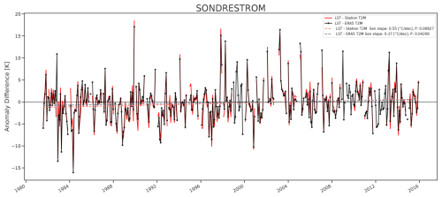
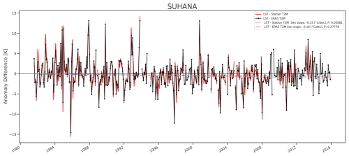
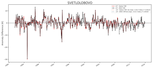
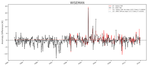
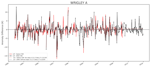
To assess the general stability of the LST dataset, the differences between the monthly anomalies of the datasets (Eqs. 4, 5 and 6) and the trends of these differences are calculated. Since high correlation values were obtained for T2M and Tair_max, these two datasets are considered for the LST stability analysis. The confidence interval is set to 95 %, meaning that trends with p values below 0.05 present a significant trend. Ideally, the trend of the difference should be zero or very close to zero. The results are shown in Table 7: 10 of the 24 trends of the anomaly differences involving LST present statistically significant trends. This indicates that for these datasets, the difference between the anomalies increases or decreases over time and, thus, is not stable. Four stations (DEWAR LAKES, SVEAGRUVA, SVETLOLOBOVO, and WISEMAN) show statistically significant trends when comparing T2M and Tair_max anomalies (e.g. see SVEAGRUVA in Fig. 8). However, these stations present stable trends for the comparison with LST anomalies. For example, the comparison of LST versus T2M at SVEAGRUVA is very stable (0.10 K per decade) (see Fig. 8). The same observation can be made at DEWAR LAKES. SVEAGRUVA is a special case as the data are very sparse. Overall, the LST–Tair_max trend and LST–T2M trends shown in Table 7 are not consistent across datasets. For example, Fig. 9 shows the trends of the anomalies at KANGERLUSSUAQ. All trends are stable (statistically non-significant), but differences are visible in the trend values for both LST comparisons. Plots of the trends of the other stations are shown in Appendix A1. Several reasons, such as orbit drift, missing data, or corrupt station data, could explain the observed discrepancies. Instabilities are also visible in the Tair versus T2M comparisons. The significant trend for the comparison of Tair versus T2M can be explained by missing station data (Appendix A1). Six of the 12 LST versus T2M experiments are statistically non-significant, suggesting no detectable trends for the anomaly differences at these stations. Regarding the Tair_max anomalies minus LST anomalies trends, 4 out of 12 stations show a significant trend. The stations located at DEWAR LAKES, KANGERLUSSUAQ, LAINIO, SUHANA, SVEAGRUVA, and WRIGLEY A do not show a significant trend in the comparisons to LST (see Table 7).

Table 7 Trend of the anomaly differences for the three pairs of differences. Trends in italic are significant (p value <0.05), and associated p values are marked in bold.

Figure 8 Monthly differences in the anomalies at SVEAGRUVA (Svalbard) between 1981 and 2015.

Figure 9 Monthly differences in the anomalies at KANGERLUSSUAQ (Greenland) between 1981 and 2015.

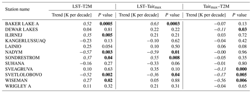
Table 8 Trends in monthly mean anomalies (K per decade) for selected stations. Values in italic are significant (p value <0.05), and associated p values are marked in bold.

LST and air temperature trends of stable stations (DEWAR LAKES, KANGERLUSSUAQ, LAINIO, SUHANA, SVEAGRUVA, and WRIGLEY A) have the same order of magnitude (Table 8), and all stations present a warming trend. DEWAR LAKES, located east of Nunavut (Canada), shows a more pronounced trend for LST than for the air temperature (Tair and T2M). Tair captured at the weather station does not present a significant trend. KANGERLUSSUAQ in Greenland shows similar trends in LST as in air temperature. LAINIO, located in a forested area in northern Scandinavia, presents similar trends to LST and Tair, while the corresponding T2M trend is lower. The LST trend in SUHANA (Siberia) does not show a significant trend for LST, but both air temperature datasets show a consistent trend. WRIGLEY A, located in the Northwest Territories in a forested area, shows a higher LST trend than T2M trend.

4.3 Analysis of summer and winter periods

To further investigate whether the orbital drift of the NOAA satellites influences the stability analysis and determined trends, the previous analysis is now performed separately for polar winter and polar summer (see Sect. 3.5). Correlation coefficients (r), trends (slopes), and p values of the differences between LST anomalies minus Tair_max anomalies and LST anomalies minus T2M anomalies are calculated.

Correlation coefficients (r) (Table 9) for summer and winter for the analysis against LST lie in the range 0.4–0.8. Correlation results are, on average, slightly higher for LST versus T2M than LST versus Tair_max, for winter and summer. SVEAGRUVA had insufficient data points in winter, and the trends for summer were not significant. Therefore, this station was removed from the analysis. Winter shows only slightly higher correlation values than summer. At BAKER LAKE A, ILIRNEJ, SONDRESTROM, and WISEMAN, r values in summer are higher than in winter. Correlation values are slightly higher for the separate seasons (Table 9) than for the general analysis (Table 6). Correlation results for the Tair_max versus T2M experiment range between 0.57 and 0.96. The lowest correlation values are obtained at WISEMAN and WRIGLEY A. All of the stations except SVETLOLOBOVO exhibit r values in a similar range in summer and winter. The air temperature correlation value at SVETLOLOBOVO is considerably lower in summer than in winter. SVETLOLOBOVO is the station located the furthest south, at 55° latitude. At WRIGLEY A, r values are similar for all significant results.

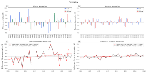
The results in the previous section show that some instabilities could be detected from the trends of the anomaly differences. The same analysis is now performed separately for summer and winter (Table 10). Five out of 12 stations do not show any significant trend either in summer or in winter. Except for SUHANA, the remaining stations only show a significant trend during summer. For example, KANGERLUSSUAQ (Table 10 and Fig. 10) presents a significant positive trend during summer but no significant trend in winter. SUHANA experiences a significant positive trend in winter for the LST anomaly minus Tair_max anomaly difference, but this trend is not observed in comparison to T2M (Table 10 and Fig. 11). From Fig. 11, it can also be noticed that the differences between Tair_max and T2M increase over time in winter and summer, which suggests discrepancies between air temperature measured at the station and from ERA5-Land. The magnitude of the LST anomalies is also generally higher than Tair and T2M magnitude (Figs. 10 and 11), which can be explained by the higher amplitude of the LST diurnal cycle pattern compared to air temperature (Good, 2016; Sharifnezhadazizi et al., 2019). SVETLOLOBOVO and KANGERLUSSUAQ present poor correlation results in summer (see Table 9) and also exhibit strong significant summer trends for the anomaly difference, contrary to winter trends that remain stable (Table 10).

Table 9 Pearson correlation coefficient (r) of the monthly anomalies for the summer and winter period.

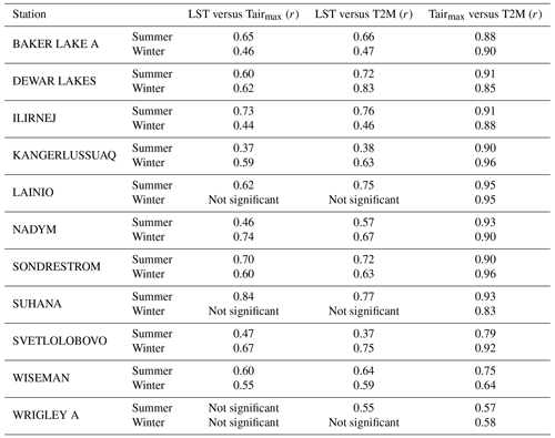
Table 10 Trends of the anomaly differences for winter and summer. Trends in bold–italic are statistically significant.

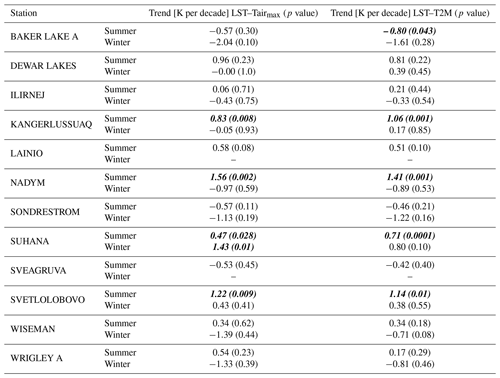
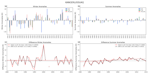
Figure 10 Winter and summer anomalies and the difference between anomalies of LST, T2M, and Tair time series for KANGERLUSSUAQ (Greenland).

Figure 11 Winter and summer anomalies and the difference between anomalies of LST, T2M, and Tair time series for SUHANA (Siberia).

4.4 LST analysis for the pan-Arctic region

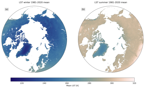
The previous sections identified a few stability issues in the current LST dataset, particularly during summer months (Tables 7 and 10). However, these limitations are not unique to LST, as analyses of the difference between both air temperature datasets also revealed instabilities (Table 7). While this highlights the stability and accuracy of the LST dataset, the trend analysis should be interpreted with care. The summer months are more prone to instability in the analysis than the winter months. Therefore, the trends of the winter and summer months are computed separately for the entire pan-Arctic region (Fig. 12). This allows us to compare and analyse temperature changes across different seasons. Additionally, mean LST values for summer and winter for the pan-Arctic are calculated (Fig. 13) to further understand temperature distributions during different seasons.

Cold glaciers and mountain zones in western Canada and Alaska are well captured in the summer mean temperatures (Fig. 13). These regions also exhibit a pronounced warming during summer and winter (Fig. 12). Warmer mean winter temperatures are present along the Lena River in Siberia, which is also visible in the mean annual ground temperature (MAGT) map from Obu et al. (2019). Generally, summer and winter mean LST values follow the temperature pattern shown in the MAGT map. For example, valleys in Russia present in the MAGT map are also visible in the mean LST values (Obu et al., 2019). The Verkhoyansk Mountains (Yakutia) present a pronounced winter warming trend. During summer that area does not show a significant temperature trend.

During the winter period, pronounced warming can also be observed in the south of Greenland as well as in eastern Canada (Fig. 12c). Vandecrux et al. (2024) analysed firn and ice temperature at 10 m below the surface (T10m) across the Greenland Ice Sheet and found a general warming trend across the ice sheet. Parts of southern Siberia show negative winter and summer trends. Similar cooling trends for winter are also visible in the AVHRR Polar Pathfinder product over Siberia, as well as warming trends along the Siberian north coast during winter (Key et al., 2016). Large areas at latitudes >70° suffer from persistent cloud cover and are not covered by satellite LST data. Summer LST trends reveal warming in the northern Siberian lowlands and the Lena Delta area. Northern Canada and most of Greenland also show warming. Cooling trends are visible in the summer period in the south of Siberia and southern Canada.

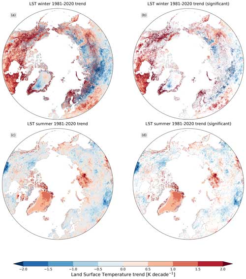
Figure 12 Panels (a) and (b) show the trends for the winter period and (c) and (d) the trends for the summer period. The left panels (a, c) show the trends independent of their significance. The right panels (b, d) show only the significant trends; i.e. areas with statistically insignificant trends (p>0.1) are masked out.

Figure 13 Mean LST (1981–2020) for (a) winter and (b) summer.

5 Discussion

5.1 Datasets

5.1.1 EUMETSAT AVHRR FDR

The AVHRR data used in this study are not considered a fundamental climate data record (FCDR) because the calibration for the thermal channels is satellite-specific, and uncertainty quantification is missing. The absence of thermal inter-calibration of the IR sensors on board AVHRR might introduce sensor discontinuities in the dataset (EUMETSAT, 2023c). Therefore, the stability of this dataset needs to be thoroughly assessed before using it for climatological analyses. Solutions to fix this issue might be implemented in the next release of the FDR. However, in the present study, sensor discontinuities were not detected. AVHRR data are affected by orbital drift and, although this effect is negligible for the Northern Hemisphere and monthly means, this still might introduce artificial trends. Different solutions to correct for orbital drift exist (Ma et al., 2020; Julien and Sobrino, 2022). However, for the moment, none of the existing LST datasets applies such a correction to the entire AVHRR time period. The present study revealed artificial trends during summer months for a few stations when compared to ERA5-Land T2M and in situ air temperature.

5.1.2 ERA5-Land T2M

T2M data from reanalyses have the advantage that they are continuous and free of data gaps. However, the coarse resolution of ERA5-Land (9 km) represents a challenge when compared with variables such as LST, which have high spatial variability and are linked to intrinsic properties of the surface such as roughness and moisture (Hulley et al., 2014). Some discrepancies between ERA5-Land T2M and the EUSTACE station Tair data are visible in the anomaly analysis (Figs. 10 and 11). Previous work performed for the Chinese Qilian Mountains (Zhao and He, 2022) found an average RMSE of 2.2 °C between ERA5-Land and air temperature measurements from weather stations, which was mainly attributed to elevation differences between both data sources. However, ERA5-Land performed well in estimating trends. Another study from the northeast of Brazil (de Araújo et al., 2022), which also compares air temperature data from stations to ERA5-Land, indicates that ERA5-Land generally underestimated average air temperature values.

5.1.3 EUSTACE Tair

EUSTACE air temperature data are homogenized and have undergone break detection and quality checks (Brugnara et al., 2019). Large parts of eastern Siberia, northern Canada, and Alaska only have a few EUSTACE weather stations in their territory (Rayner et al., 2020). In general, stations are placed close to settlements and road access, meaning it is difficult to obtain quality weather station data from remote places. Satellite imagery represents, therefore, a valuable source for obtaining temperature data from remote places. In the current study, many stations were discarded due to their proximity to large water bodies or the coast, which would impact the comparison with remote sensing data. In Greenland, two EUSTACE stations are located in close vicinity to each other (KANGERLUSSUAQ and SONDRESTROM). However, they present very different results when compared to ERA5-Land data and satellite data (see Tables 7 and 9). Both stations are assigned to different ERA5-Land and satellite pixels. This area in Greenland is composed of deep fjords with steep hillslopes, which might not be captured well by the spatially coarse model data and satellite data.

5.1.4 Pan-Arctic AVHRR LST

The AVHRR LST dataset developed in this study covers 40 years and represents a valuable data source, complementing data from models and weather stations for obtaining temperature information at a hemispheric scale. A dynamic snow and vegetation cover mask is integrated into the LST algorithm to assign correct emissivities to snow-covered pixels. This is particularly important for cryospheric research at high latitudes. Most of the existing LST datasets do not use a dynamic snow mask and assign snow emissivity based on a static LSE map (Ma et al., 2020). Snow cover onset and snow melt onset are events that can be captured by satellite thermal imagery and are of particular interest for the thermal regime of the ground (Grünberg et al., 2020; Hammar et al., 2023). Westermann et al. (2012) highlighted the importance of using an accurate cloud mask when using LST data for permafrost modelling, as this can lead to high uncertainties and a lack of accuracy. The pan-Arctic AVHRR LST dataset incorporates the latest cloud mask from the CLARA-A3 database (Karlsson et al., 2023b), and a low cloud probability threshold (see Sect. 3) was used to avoid cloud contamination.

LST trends computed at different stations (Table 8) are positive and lie in the same ranges as trends computed for Tair and T2M. Furthermore, LST temperature trend maps (Fig. 12) highlight areas that are particularly sensitive to Arctic amplification and present pronounced warming trends. LST trends computed for the summer and winter periods at a hemispheric scale reveal distinct warming areas as well as some regions with cooling trends. Maturilli et al. (2019) determined air temperature trends from weather station data in Ny-Ålesund (Svalbard) from 1993 to 2017 and found that the strongest warming trend occurred during the winter season. They found a summer warming trend of +0.6 K per decade, which corresponds to the LST warming trend for Svalbard shown in Fig. 12. Compared to air temperature trends, satellite-derived LST trends can present a cold bias as only clear-sky days are considered in the LST generation (Westermann et al., 2017). Therefore, the all-sky LST trends might be even higher. All-weather LST datasets have been generated in the past by combining energy balance modelling or reanalysis LST data with LST TIR data (Martins et al., 2019; Zhang et al., 2021).

5.2 Point to pixel comparison

The landscape in the pan-Arctic region is very heterogeneous; for example, complex wetland systems are difficult to map from satellite imagery (Olefeldt et al., 2021; Palmtag et al., 2022). Land cover data such as from the CCI project are thus prone to high uncertainties in the high northern latitudes (Bartsch et al., 2024). The nominal spatial resolution of AVHRR GAC pixel is 4 km. Air temperature measured at a nearby location might differ considerably from the corresponding AVHRR LST and depends on vegetation type and water content of the ground.

5.3 Comparison of LST, Tair, and T2M

Day length and, consequently, solar irradiance cover a wide range in the Arctic. During winter, there is constant night, and Tair is in close agreement with LST (Hachem et al., 2012; Urban et al., 2013). Furthermore, during winter, most of the pan-Arctic region is covered by snow. Snow cover variations directly influence LST (Thiebault and Young, 2020). LST and air temperature anomalies exhibit a strong correlation (mean (r) >0.6), and LST anomalies show a similar pattern to air temperature anomalies (Figs. 10 and 11). LST anomalies present a greater magnitude, which can be explained by a greater amplitude in the LST diurnal cycle than in the air temperature diurnal cycle. Differences in winter anomalies are more pronounced than summer anomalies. This can be explained by the clear-sky bias that occurs in satellite LST data (Westermann et al., 2012): cloud cover affects the winter period more than the summer period. Such a cooling bias was also observed over the Greenland Ice Sheet over ice surface temperature (Hall et al., 2012). Regarding monthly means, the air temperature mean is higher than the LST mean value, which only considers clear-sky days. Under cloudy skies, air and surface temperature are in close agreement (Obu et al., 2019). A few missing data occurred in the EUSTACE, which made the ERA5-Land data more reliable for such an analysis. However, EUSTACE records two temperatures per day: T_max and T_min. Therefore, for analysis at daily frequency, EUSTACE might be more suitable, especially for satellites having an overpass time close to noon. Winter data proved to be stable over all investigated stations. This makes this dataset particularly interesting for studying the winter months in the high latitudes. The winter period is a particularly active time for the ecosystem in the Arctic (Berge et al., 2015), but it tends to be understudied.

Finally, trends for the three different datasets computed at stations with good temporal stability (Table 8) showed good agreement, with LST trends generally exhibiting stronger positive trends than air temperature. In addition, LST winter trends for central Siberia (Fig. 12) showed similar values as in Waring et al. (2023). Strong summer warming in the north of the Krasnoyarsk region and northern Nunavut (Canada) (visible in Fig. 12d) is also visible in ERA5-Land temperature data for the period 1984–2022 in the work of Larocca et al. (2024). The regions showing positive trends in LST are generally associated with lichens, moss, and herbaceous land cover, whereas regions with negative trends are mostly located in forested areas. Mildrexler et al. (2011) revealed the cooling effect of forests on LST, which might slow the general temperature increase in the Arctic. The presence of thermokarst lakes and wetlands as depicted in Olefeldt et al. (2021) might also slow the warming trends slightly. The Yamal Peninsula, for example, contains many water bodies and thermokarst lakes and shows a slower warming trend than an area with a majority of barren soil. Hemispheric LST data can also be used to highlight fast-warming areas that might lead to abrupt permafrost thaw, which in turn influences carbon fluxes (Treat et al., 2024). LST also has the advantage over air temperature of being more sensitive to changes in vegetation density (Mildrexler et al., 2011), which makes LST a particularly interesting variable for cryospheric research.

6 Conclusions

This study presents the workflow to derive a pan-Arctic LST dataset from the EUMETSAT AVHRR GAC FDR and validates the new LST product against in situ LST. AVHRR LST is derived with the generalized split-window algorithm (Wan and Dozier, 1996), and the corresponding RTM is performed with RTTOV v.13, based on a new calibration database (Ermida and Trigo, 2022). This ensures an optimal representation of atmospheric conditions in the pan-Arctic region. This LST dataset utilizes a recent cloud mask with notable improvements compared to previous cloud products (Karlsson et al., 2023b), which is of particular importance for LST retrieval. The pan-Arctic AVHRR LST product showed good performance, and validation results lie in the range of similar products. The new LST product is assessed for stability in the pan-Arctic region by comparing it to air temperature data from weather stations and T2M data from ERA5-Land. Twelve weather stations belonging to the EUSTACE global station dataset are chosen based on several criteria: latitude >50° N, a minimum of 30 years of overlapping data, and homogeneous land cover over at least 1 GAC pixel. LST trends and variability are compared to ERA5-Land T2M and EUSTACE Tair maximum data. The correlation coefficients between the datasets indicate good agreement: r >0.9 for the monthly mean correlation and ∼0.5 to ∼0.8 for the anomaly analysis. The analysis of the differences in anomalies showed slightly significant trends for the summer months but no artificial trends in the data during the winter months when solar irradiance is absent. LST trends for the winter and summer periods were computed for the entire pan-Arctic region and revealed spatially varying trends. In winter, positive trends in the south of Greenland, Siberia, and eastern Canada were revealed. Summer temperature trends highlight the fast warming of the Greenland Ice Sheet and a large region in the vicinity of the Lena Delta. Its good accuracy and emissivity retrieval based on dynamical vegetation and snow masks make this product suitable for a wide range of research applications in the pan-Arctic region. However, future research investigate a possible spatial upsampling of the dataset (e.g. to 1 km spatial resolution). Orbital drift correction with a robust method would allow one to extend the study to lower latitudes.

Appendix A: Anomaly differences

Figure A1 Differences in the anomalies at BAKER LAKE A (Canada) as a time series.

Figure A2 Differences in the anomalies at DEWAR LAKES (Canada) as a time series.

Figure A3 Differences in the anomalies at ILIRNEJ (eastern Siberia) as a time series.

Figure A4 Differences in the anomalies at LAINIO (Norway) as a time series.

Figure A5 Differences in the anomalies at NADYM (Siberia) as a time series.

Figure A6 Differences in the anomalies at SONDRESTROM (Greenland) as a time series.

Figure A7 Differences in the anomalies at SUHANA (Siberia) as a time series.

Figure A8 Differences in the anomalies at SVETLOLOBOVO (Siberia) as a time series.

Figure A9 Differences in the anomalies at WISEMAN (Canada) as a time series.

Figure A10 Differences in the anomalies at WRIGLEY A (Alaska) as a time series.