The evolution of Arctic permafrost over the last 3 centuries from ensemble simulations with the CryoGridLite permafrost model

Understanding the future evolution of permafrost requires a better understanding of its climatological past. This requires permafrost models to efficiently simulate the thermal dynamics of permafrost over the past centuries to millennia, taking into account highly uncertain soil and snow properties. In this study, we present a computationally efficient numerical permafrost model which satisfactorily reproduces the current ground temperatures and active layer thicknesses of permafrost in the Arctic and their trends over recent centuries. The performed simulations provide insights into the evolution of permafrost since the 18th century and show that permafrost on the North American continent is subject to early degradation, while permafrost on the Eurasian continent is relatively stable over the investigated 300-year period. Permafrost warming since industrialization has occurred primarily in three “hotspot” regions in northeastern Canada, northern Alaska, and, to a lesser extent, western Siberia. We find that the extent of areas with a high probability (p_3 m>0.9) of near-surface permafrost (i.e., 3 m of permafrost within the upper 10 m of the subsurface) has declined substantially since the early 19th century, with loss accelerating during the last 50 years. Our simulations further indicate that short-term climate cooling due to large volcanic eruptions in the Northern Hemisphere in some cases favors permafrost aggradation within the uppermost 10 m of the ground, but the effect only lasts for a relatively short period of a few decades. Despite some limitations, e.g., with respect to the representation of vegetation, the presented model shows great potential for further investigation of the climatological past of permafrost, especially in conjunction with paleoclimate modeling.

1 Introduction

With an estimated area of 12 to 17 million km² (Gruber, 2012; Chadburn et al., 2017; Obu et al., 2019), permafrost is the largest non-seasonal component of the Earth's cryosphere. Permafrost is a characteristic factor of Arctic and subarctic ecosystems and determines a variety of fundamental hydrological and biogeochemical processes (Walvoord and Kurylyk, 2016; Turetsky et al., 2020). The occurrence and thermal state of permafrost are determined by long-term local climate history (French and Millar, 2014). In particular, the thermal state of the deeper soil layers (i.e., in depths of tens to hundreds of meters) must be considered a legacy of a past climate (e.g., Lachenbruch and Marshall, 1986; Allen et al., 1988; Osterkamp and Gosink, 1991; Harrison, 1991; Kneier et al., 2018). Permafrost in some places has survived substantial changes in climate and sea levels during past glacial–interglacial cycles (Froese et al., 2008), with the oldest known permafrost existing for at least 650 000 years (Murton et al., 2022). The glacial history has a lasting effect on present-day deep ground temperatures and ground ice conditions through climatic and geomorphological processes. Cold climatic conditions during the past tens to hundreds of thousands of years, in combination with sedimentation, led to accumulation of ground ice and organic carbon at increasing soil depths (Kanevskiy et al., 2017). Although it is assumed that most of the ground ice and organic material occur near the surface (<3 m) (Hugelius et al., 2014) deeper reservoirs of organic carbon and ground ice do exist and control the long-term thaw sensitivity of permafrost landscapes (West and Plug, 2008). For the Alaskan coastal plain, Péwé (1979) estimated that pore ice and segregated ground ice comprise 41 % by volume of the soil at depths between 3 and 10 m. Ice wedges extend even deeper into the ground, with very deep and massive deposits of ground ice and carbon found in the Yedoma deposits of Siberia and Alaska, reaching depths over 50 m (Kanevskiy et al., 2011; Strauss et al., 2021). The presence of ground ice and carbon at greater soil depths demands a better understanding of the thermal state of deep permafrost and its sensitivity to climatic changes.

Reconstruction of the climatically induced thermal state of permafrost at or beyond the depth of zero annual amplitude demands simulation times of centuries to millennia to achieve a dynamic equilibrium that can be considered largely unaffected by initial conditions (e.g., Ross et al., 2021). This requires computationally efficient models, in particular if large regions represented by many grid cells are to be evaluated. In addition, it is important that such models can operate with limited and highly uncertain information about thermal and hydrological ground properties. In particular, groundwater and ground ice contents are highly uncertain but strongly affect heat uptake and storage in the ground. Such uncertainties can be addressed with probabilistic approaches such as parameter ensemble simulations (e.g., Schneider von Deimling et al., 2006; Murphy et al., 2007), which allow simulations to be evaluated with the consideration of plausible parameter ranges. However, simulations of a large number of ensemble members require efficient computations and prefer a small amount of required input data. The same is true for other probabilistic model applications such as data assimilation and hybrid modeling (e.g., Madadgar and Moradkhani, 2014; Kraft et al., 2022). Furthermore, climate reconstructions usually provide only large-scale air temperature and precipitation data, while other near-surface climate variables such as wind speed, air pressure, specific humidity, and radiation are difficult to obtain, in particular at high temporal resolution. This severely limits the options for model forcing and hence process representation (e.g., due to unclosed surface energy and water balances). Simulations targeting the long-term evolution of deep permafrost therefore impose certain requirements and constraints on the model used.

Numerous permafrost models are available ranging from analytical steady-state solutions (e.g., Gruber, 2012; Obu et al., 2019) to very sophisticated thermo-hydrological numerical models (e.g., Kurylyk and Watanabe, 2013; Karra et al., 2014; Atchley et al., 2015; Westermann et al., 2023). The latter usually require an immense computational effort for experiments spanning hundreds of years and are therefore typically used for local to regional process studies covering periods between years and decades. In contrast, pan-Arctic permafrost simulations, such as those performed with Earth system models (ESMs), typically comprise several hundreds of years for historical and future climate projections. Many land surface schemes from ESMs cannot capture the long-term thermal evolution of deep permafrost since their representation of the ground is often limited beyond the upper 3 to 10 m of the subsurface (Hermoso de Mendoza et al., 2020; Steinert et al., 2021). To date, there are only few permafrost modeling approaches that focus on paleoclimatic periods (e.g., Crichton et al., 2014; Willeit and Ganopolski, 2015; Schneider von Deimling et al., 2018; Kitover et al., 2019; Saito et al., 2021). The ability of such models to perform simulations over millennia comes at the price of a very limited representation of processes and low spatial and temporal resolution.

Here, we present and evaluate a computationally efficient numerical permafrost model (CryoGridLite) designed to provide insights into the evolution of the thermal state of permafrost and active layer thickness over many centuries for the Arctic permafrost region. With the CryoGridLite model, we aim to bridge the gap between very sophisticated permafrost process models and reduced schemes used for paleoclimatic simulations. Compared to comprehensive process models like CryoGrid3 (Westermann et al., 2016) or the CryoGrid Community Model (Westermann et al., 2023), CryoGridLite is approximately 3 orders of magnitude faster, enabling the execution of long-term simulations spanning hundreds to thousands of years. The enhanced efficiency is achieved through two key components: (i) the utilization of an implicit solution scheme and (ii) a streamlined representation of the underlying processes. Our approach aligns with the objective of providing plausible ranges of permafrost states rather than focusing on highly precise results for specific locations. This is accomplished through the application of multi-parameter ensemble simulations, which have become feasible due to the substantial enhancements achieved in computational efficiency. By employing this methodology, we can capture a broader range of potential permafrost conditions, encompassing the inherent uncertainties and variability associated with real-world scenarios. In the simulations we account for uncertainties in soil parameters such as water and ice content, as well as uncertainties in snowpack properties.

Based on observations, we investigate the ability of the new model to reproduce the current thermal state of permafrost as determined by the climatic evolution over the last centuries (1700–2020). The required model parameters are greatly reduced compared to permafrost process models and are based entirely on pan-Arctic or global datasets. Model forcing is limited to daily mean surface temperature, precipitation, and geothermal heat flux. Specifically, we evaluate the applicability and performance of the model to represent the current permafrost temperatures to a depth of 10 m and its trend over recent decades based on long-term temperature records from boreholes. In addition, we use observations of the thickness of the active layer to evaluate the model's ability to reproduce annual freeze–thaw dynamics. In addition, we apply the model to trace the evolution of Arctic permafrost extent over the past 3 centuries.

2 Methods

CryoGridLite largely adopts schemes and parameterizations previously implemented and tested in the context of regional and local permafrost modeling using CryoGrid2 (Westermann et al., 2011; Langer et al., 2013; Westermann et al., 2017) and CryoGrid3 (Westermann et al., 2016). CryoGridLite consists of (i) a ground module that calculates conductive heat transfer with phase change within the soil and bedrock and (ii) a dynamic snow scheme to represent the insulating effect of seasonal snow cover. Furthermore, some data prepossessing is demanded in order to derive gridded soil stratigraphies and snow parameters by synthesizing different global datasets, as well as to generate offline model forcings based on global reanalysis data and paleoclimate simulations.

2.1 Ground heat transfer and phase change

In contrast to its predecessors, CryoGrid2 and CryoGrid3, CryoGridLite solves the nonlinear heat equation with phase change in terms of enthalpy density (volumetric enthalpy) instead of temperature:

$$\begin{array}{}\text{(1)}& {\displaystyle \frac{\partial H_{\mathrm{v}}\left(T\right)}{\partial t}}-{\mathrm{\nabla }}_z\left[K\left(T\right){\mathrm{\nabla }}_{z}T\right]=\mathrm{0},\end{array}$$

where H_v [J m⁻³] is the volumetric enthalpy as an invertible function of temperature T [K], z [m] is depth along the vertical axis, t [s] is time, and K(T) [W m⁻¹ K⁻¹] is the temperature-dependent thermal conductivity. Equation (1) can be solved using the iterative backward Euler scheme given by Swaminathan and Voller (1992):

$$\begin{array}{}\text{(2)}& {\displaystyle }{\mathit{\alpha }}_j^i{T}_{j-\mathrm{1}}^{i+\mathrm{1}}-{\mathit{\beta }}_j^i{T}_j^{i+\mathrm{1}}+{\mathit{\gamma }}_i^i{T}_{j+\mathrm{1}}^{i+\mathrm{1}}+b_j^i-{\displaystyle \frac{{H_{\mathrm{v}}}_j^{i+\mathrm{1}}-{H_{\mathrm{v}}}_j^{\mathrm{0}}}{\mathrm{\Delta }t}}=\mathrm{0},\end{array}$$

with

$$\begin{array}{}\text{(3)}& {\displaystyle \frac{{H_{\mathrm{v}}}_j^{i+\mathrm{1}}-{H_{\mathrm{v}}}_j^{\mathrm{0}}}{\mathrm{\Delta }t}}={\left({\displaystyle \frac{\mathrm{d}{H}_{\mathrm{v}}}{\mathrm{d}T}}\right)}_j^i{\displaystyle \frac{T_j^{i+\mathrm{1}}-T_j^i}{\mathrm{\Delta }t}}+{\displaystyle \frac{{H_{\mathrm{v}}}_j^i-{H_{\mathrm{v}}}_j^{\mathrm{0}}}{\mathrm{\Delta }t}},\end{array}$$

where Δt [s] is a constant time step, T [K] is the temperature, α, β, and γ [J m⁻³ K⁻¹ s⁻¹] are pre-factors determined by the temporal invariant grid cell spacing and variable thermal conductivities, and b [J m⁻³ K⁻¹ s⁻¹] is an optional energy source term which can be used to apply an external forcing. The index j marks the grid cell number increasing with depth, and the index i indicates the iteration step. The iteration step i=0 indicates the state of the previous time step (t−1), which is updated to the current time step (t) after reaching convergence.

At each time step, iteration continues until the temperature profile matches the inverse enthalpy profile controlled by a tolerance parameter which we set to $\mathrm{1}\times {\mathrm{10}}^{-\mathrm{3}}$ K. The release and uptake of latent heat during phase change are accounted for by the derivative of the enthalpy function, $\frac{\mathrm{d}{H}_{\mathrm{v}}}{\mathrm{d}T}$. We choose the form of the enthalpy function to follow the freezing characteristic of pure water (i.e., “free” water; for details, see Appendix A). This has the benefit of providing a readily available inverse function (Eq. A3), which is necessary for the iterative scheme, at the cost of neglecting complex interactions of the freezing characteristic with soil composition, structure, and chemistry (Koopmans and Miller, 1966). For each grid cell the ground thermal properties such as thermal conductivities and heat capacities are calculated based on the ground composition defined by the volumetric contents of organics, minerals, pore water, and pore ice (see Sect. 2.2.2). We note that the thermal properties of excess ground ice are not considered here but are considered in a companion study by Nitzbon et al. (2023) using the same model. The upper boundary condition is defined by an external surface temperature, while the lower boundary condition is defined by a locally constant geothermal heat flux (Davies, 2013). In rare cases in which convergence cannot be reached within a maximum of 500 iterations, the maximum temperature deviation is printed out as a warning before the next time step is calculated. It is, however, important to note that such a temperature deviation only indicates that the current temperature profile is not consistent with the enthalpy profile. This deviation does not affect energy conservation over the total profile but indicates that the distribution of energy within the profile is not exact.

The numerical performance and stability of the applied implicit method are evaluated in comparison with commonly used numerical integration methods: Crank–Nicolson and TRBDF2 (second-order diagonally implicit Runge–Kutta methods), Radau IIA5 (fifth-order fully implicit tableau method), Heun (canonical explicit trapezoidal method), and SSPRK43 (fourth-order stability-preserving explicit Runge–Kutta method). The test simulations under periodic freeze–thaw conditions result in a mean absolute error of about 0.014 K for time steps of 24 h. With this acceptable level of accuracy, the CryoGridLite scheme is about an order of magnitude faster than the other numerical integration schemes. More details about the numerical accuracy and performance are provided in Appendix C and by Swaminathan and Voller (1992). We further note that the implicit time stepping scheme employed in this work bears some resemblance to a recently proposed method (Tubini et al., 2021) which applies the Newton–Casuli–Zanolli algorithm (Casulli and Zanolli, 2010) to solve the nonlinear heat equation in enthalpy form. The primary advantage of the applied scheme is that it is found to be generally stable using daily time steps while still being energy-conserving. It is furthermore capable of representing the latent heat effect via a simplified freezing characteristic without requiring the computationally demanding task of explicitly tracking the position of freezing fronts. We note that the implicit solver used is strictly valid only for phase change within a homogeneous material. However, we point out that any uncertainties due to natural heterogeneities at the surface and in the subsurface on the spatial scales considered are likely to be larger than the errors introduced by a generalized representation of the heat transfer process. Conservation of energy is the primary concern for long-term simulation between centuries and millennia.

2.1.1 Snowpack representation

The snowpack is an important factor controlling the thermal state of permafrost and induces large uncertainties in permafrost modeling in general (Langer et al., 2013; Gouttevin et al., 2018; Jan and Painter, 2020). The insulating effect of the snowpack must therefore be carefully represented, although very coarse spatial model resolutions and reduced forcing data limit the ability to simulate complex processes determining the snow properties. CryoGridLite simulates the insulative effect of the snowpack using a bulk approach based on daily snowfall rates and snow properties that are defined by five climate regions following Sturm et al. (2010). Snow accumulates on top of the ground domain according to snowfall. For this purpose, empty ghost cells on top of the ground domain are populated by snow with an initial snow density according to snow depth. The snow depth is updated at the beginning of each time step as

$$\begin{array}{}\text{(4)}& \begin{array}{rl}{h}_{\mathrm{snow}}^t& =\left(h_{\mathrm{snow}}^{t-\mathrm{1}}-\mathrm{\Delta }{h}_{\mathrm{melt}}^{t-\mathrm{1}}+P_{\mathrm{snow}}^t\mathrm{\Delta }t{\displaystyle \frac{{\mathit{\rho }}_{\mathrm{water}}}{{\mathit{\rho }}_{\mathrm{snow},\min }}}\right)\\ & {\displaystyle \frac{{\stackrel{\mathrm{‾}}{\mathit{\rho }}}_{\mathrm{snow}}^t}{{\mathit{\rho }}_{\mathrm{snow},\mathrm{snow}}^t}}{\mathit{\rho }}_{\mathrm{snow},\mathrm{bulk}}^t,\end{array}\end{array}$$

where h_snow [m] is the snow depth, Δh_melt [m] is the change in snow depth due to melting, P_snow [m s⁻¹] is the snowfall rate, ρ_water [kg m⁻³] is the density water (set to 1000 kg m⁻³), ρ_snow,min is the initial snow density, ${\stackrel{\mathrm{‾}}{\mathit{\rho }}}_{\mathrm{snow}}$ is the average density of the actual snowpack, and ρ_snow,bulk is the bulk snow density predicted according to Sturm et al. (1995) as

$$\begin{array}{}\text{(5)}& \begin{array}{rl}{\mathit{\rho }}_{\mathrm{snow},\mathrm{bulk}}^t& =({\mathit{\rho }}_{\mathrm{snow},\max }-{\mathit{\rho }}_{\mathrm{snow},\min })(\mathrm{1}-e^{-k_{\mathrm{1}}{h}_{\mathrm{snow}}^t-k_{\mathrm{2}}{d}^t})\\ & +{\mathit{\rho }}_{\mathrm{snow},\min },\end{array}\end{array}$$

where ρ_snow,max is the maximum snow density, k₁ and k₂ are empirical snow densification factors, and d indicates the day count of the snow season. All snow parameters are set according to values introduced by Sturm et al. (2010) defined by a global map of snow climate zones. The snow density of each grid cell is scaled so that the average density of the actual snowpack matches the predicted bulk snow density. This procedure generates a layered snowpack over time with the highest densities for old snow layers at the bottom of the snowpack. Heat transfer and phase change in the snowpack are calculated simultaneously with the ground using the implicit scheme described above. The ablation of the snow cover is calculated with a positive degree-day approach very similar to Tsai and Ruan (2018). The snow scheme further accounts for meltwater infiltration and refreezing similar to Westermann et al. (2011) using a diagnostic bucket scheme. The bucket scheme assumes instantaneous meltwater routing if a maximum water-holding capacity of snow is exceeded. Water that exceeds a maximum value of water saturation is routed away so that ponding of meltwater is precluded. A maximum snow depth is defined by a threshold value (h_snow,max) which can be used to emulate wind-induced snow depth limitation as observed, for example, on ice-covered lakes (Sturm and Liston, 2003) or other wind-exposed parts of the landscape. The snow scheme is restricted to simulating seasonal snow by setting snow depth to zero in August of each simulation year. The build-up of multi-annual snowpacks is thus precluded. While the assumption of a predominately seasonal snow cover is true for about 95 % of the Arctic permafrost region (e.g., Fontana et al., 2010; Trishchenko and Wang, 2018), studies suggest that during the “Little Ice Age” the Canadian high Arctic islands were more substantially characterized by perennial snowfields (Andrews et al., 1976) and glaciers (Williams, 1978). It is important to note that this has implications for the interpretation of the model results, as the snow scheme used may not fully capture conditions in the very high latitudes and mountainous regions that may have been affected by year-round snowpacks, ice fields, or glaciers. Furthermore, the snow scheme used in this study has limitations in reflecting the local and complex thermal properties of snow. Specifically, the scheme does not explicitly account for processes such as wind compaction and lateral redistribution of snow due to local topographic variability, nor does it explicitly represent local interactions with vegetation. The empirical parameterization used accounts only for regional variability in bulk snow density and its compaction behavior.

2.2 Ground stratigraphies

2.2.1 Subsurface layers and vertical model grid

The ground stratigraphy is represented by six ground layers characterized by different volume fractions of soil constituents (Fig. 1). Thereby two constant layer boundaries (z_SOC30, z_SOC300) are defined according to the soil layers specified in the Northern Circumpolar Soil Carbon Database v2 (NCSDv2) (Hugelius et al., 2013). Three spatially variable soil layer boundaries marking the root zone (z_R), vadose zone (z_V), and saturated zone (z_S) are defined by soil thickness data from the Gridded Global Data Set of Soil Thickness (Pelletier et al., 2016) and specifications of the water table (see Sect. 2.3). Below z_S, a bedrock layer extends down to the end of the vertical model domain.

Regardless of the soil layers described above, the vertical model domain used for numerical integration is discretized into about 400 cells from the surface at z=0 m to a maximum depth of 550 m. The spacing of the grid cells increases with depth in an approximately logarithmic fashion, allowing a very high vertical resolution of 0.01 m near the surface, while the lowest grid cells are 100 m thick. To represent the temporal accumulation of snow above the ground surface, the vertical grid contains 200 additional ghost cells that allow the snow layer to be simulated at a vertical resolution of 0.01 m.

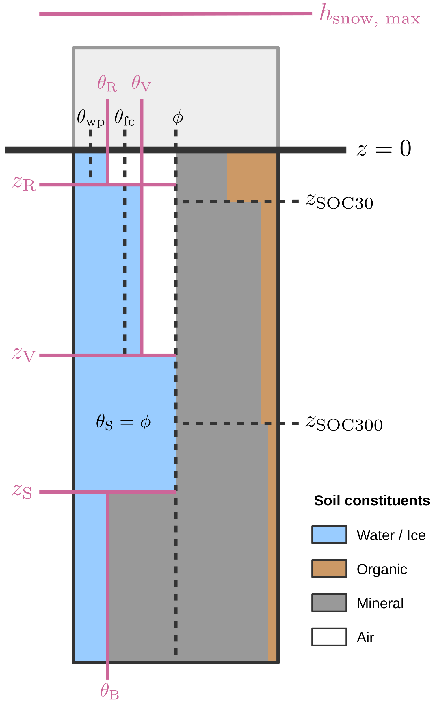
Figure 1 Schematic illustration of the applied ground stratigraphy determined by the volumetric ground constitutes, derived based on various global datasets. Layer boundaries that control the vertical distribution of groundwater, ground ice, and snow (marked in red) are randomly varied to generate a parameter ensemble. This way a wide range of plausible hydrological conditions is represented by the performed simulations. See Table 1 for the meaning of the symbols.

2.2.2 Soil stratigraphy

The vertical distribution of the ground constituents is specified based on parameterizations used for the SURFEX land surface and ocean scheme (Masson et al., 2013). The SURFEX parameterization approximates a profile of the organic soil fraction as

$$\begin{array}{}\text{(6)}& {\displaystyle }{f}_{\mathrm{o}}^i={\displaystyle \frac{{\mathit{\rho }}_{\mathrm{SOC}}^i}{(\mathrm{1}-{\mathit{\varphi }}_{\mathrm{o}}^i){\mathit{\rho }}_{\mathrm{om}}}}\end{array}$$

and a profile of the mineral soil fraction as

$$\begin{array}{}\text{(7)}& {\displaystyle }{f}_{\mathrm{m}}^i=\mathrm{1}-f_{\mathrm{o}}^i,\end{array}$$

where the index i denotes the ground layers, ρ_SOC is the soil organic carbon density, ρ_om is the pure organic matter density set to 1300 kg m⁻³, and ϕ_o [kg m⁻³] is the volumetric porosity of organic soil organic soil decreasing from 0.93 to 0.84 with depth following a power function (see the Supplement in Masson et al., 2013). Despite the fact that the model does not include a water balance scheme, we use hydrological soil parameters (wilting point – θ_wp, field capacity – θ_fc) to specify the vertical water and ice distribution within the ground (see Sect. 2.3). In this context, the power function used to scale the organic soil porosity with depth is also applied to scale the organic soil wilting point (θ_wp,o) between 0.07 and 0.22 and the organic soil field capacity (θ_fc,o) between 0.37 and 0.72. The required data on soil organic carbon density are taken from the NCSDv2 (Hugelius et al., 2013).

The mineral soil porosity (ϕ_m), the wilting point (θ_wp,m), and the field capacity (θ_fc,m) were approximated based on the SURFEX parameterizations as (see Supplement to Masson et al., 2013)

$$\begin{array}{}\text{(8)}& {\displaystyle }{\mathit{\varphi }}_{\mathrm{m}}& {\displaystyle }=\mathrm{0.49}-\mathrm{0.11}{f}_{\mathrm{sand}},\text{(9)}& {\displaystyle }{\mathit{\theta }}_{\mathrm{wp},\mathrm{m}}& {\displaystyle }=\mathrm{0.37}\sqrt{f_{\mathrm{clay}}},\text{(10)}& {\displaystyle }{\mathit{\theta }}_{\mathrm{fc},\mathrm{m}}& {\displaystyle }=\mathrm{0.45}(f_{\mathrm{clay}}{)}^{\mathrm{0.3496}},\end{array}$$

with the fractions of sand and clay obtained from the Open-ECOCLIMAP database (Masson et al., 2003; Faroux et al., 2013). The combined soil porosities (ϕ), field capacities (θ_fc), wilting points (θ_wp), volumetric mineral contents (θ_m), and volumetric organic contents (θ_o) are then calculated as weighted means of the organic and mineral soil fractions:

$$\begin{array}{}\text{(11)}& {\displaystyle }{\mathit{\varphi }}^i& {\displaystyle }=f_{\mathrm{o}}^i{\mathit{\varphi }}_{\mathrm{o}}^i+f_{\mathrm{m}}^i{\mathit{\varphi }}_{\mathrm{m}},\text{(12)}& {\displaystyle }{\mathit{\theta }}_{\mathrm{fc}}^i& {\displaystyle }=f_{\mathrm{o}}^i{\mathit{\theta }}_{\mathrm{fc},\mathrm{o}}^i+f_{\mathrm{m}}^i{\mathit{\theta }}_{\mathrm{fc},\mathrm{m}},\text{(13)}& {\displaystyle }{\mathit{\theta }}_{\mathrm{wp}}^i& {\displaystyle }=f_{\mathrm{o}}^i{\mathit{\theta }}_{\mathrm{wp},\mathrm{o}}^i+f_{\mathrm{m}}^i{\mathit{\theta }}_{\mathrm{wp},\mathrm{m}},\text{(14)}& {\displaystyle }{\mathit{\theta }}_{\mathrm{o}}^i& {\displaystyle }=f_{\mathrm{o}}^i(\mathrm{1}-{\mathit{\varphi }}_{\mathrm{o}}^i),\text{(15)}& {\displaystyle }{\mathit{\theta }}_{\mathrm{m}}^i& {\displaystyle }=f_{\mathrm{m}}^i(\mathrm{1}-{\mathit{\varphi }}_{\mathrm{m}}).\end{array}$$

The water and ice contents (θ_w) of the different soil layers are varied during parameter ensemble simulations (see Sect. 2.3) within constraints provided by the hydrological parameters above (see Table 1). The bedrock layer is represented by a purely mineral soil layer with reduced water and ice content.

2.2.3 Ground thermal properties

The thermal properties of the subsurface layers (thermal conductivity and volumetric heat capacity) are parameterized based on their composition following Westermann et al. (2013). Both volumetric heat capacity and the thermal conductivity are functions of the volumetric fractions of the ground constituents. The volumetric heat capacity C_v is calculated as a weighted arithmetic mean as

$$\begin{array}{}\text{(16)}& {\displaystyle }{C}_{\mathrm{v}}=\sum _{n=\mathrm{1}}^N{\mathit{\theta }}_n{c}_n,\end{array}$$

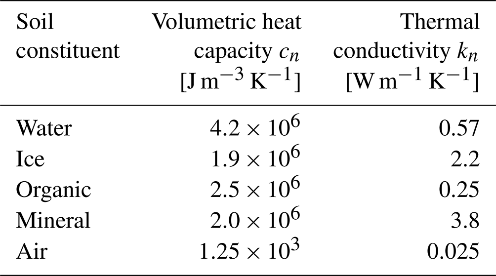
where N is the total number of soil constitutes in the mixture, θ_n is the volumetric content of the nth soil constituent, and the volumetric heat capacity of each soil constituent c_n is set according to values provided in Table B1.

The thermal conductivity is approximated using a quadratic parallel model (Cosenza et al., 2003) as

$$\begin{array}{}\text{(17)}& {\displaystyle }K={\left(\sum _{n=\mathrm{1}}^N{\mathit{\theta }}_n\sqrt{k_n}\right)}^{\mathrm{2}},\end{array}$$

and the thermal conductivity of each soil constituent is set to values provided in Table B1 in Appendix B. Note that the thermal conductivity model can be easily replaced by any other model used to approximate multiphase thermal conductivities of the ground.

2.3 Parameter ensemble simulations

Since CryoGridLite does not have a dedicated hydrology scheme and because of the low confidence in the available datasets and parameterizations on groundwater and ground ice contents at high latitudes, we apply parameter ensemble simulations to represent a wide range of hydrological conditions. Here, the relevant factors controlling the vertical water and ice distribution in the ground profile are randomly varied within realistic ranges. In this way, an ensemble of n_ens=50 randomly sampled independent parameter settings is simulated for each model grid cell.

The default groundwater and ground ice content in the subsurface is parameterized such that it reflects average hydrological conditions. For this we distinguish four hydrologically different zones in the subsurface: the root zone (R), the vadose zone (V), the saturated zone (S), and the bedrock zone (B) (see Fig. 1). By default (i.e., during model spin-up), the water content is set halfway between the wilting point and the field capacity of the respective soil layer(s) in the root zone and halfway between field capacity and porosity in the vadose zone. In the saturated zone, the ground layers are always completely saturated. In addition, we assume a saturated bedrock zone which starts at a depth derived from the Gridded Global Data Set of Soil Thickness (Pelletier et al., 2016). Below this depth (z_S), the water and ice content is reduced in favor of an increased mineral content. The default parameters defining the groundwater and ice contents are provided in Table 1.

Table 1 Overview of the parameters which were varied in the parameter ensemble simulations. The parameters were independently drawn from a uniform distribution between the respective minimum and maximum values. Here, Z_mean and Z_max refer to the mean and max soil thickness, respectively.

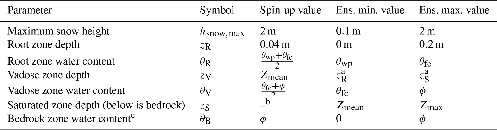
^a Needs to be sampled before z_V. ^b Extends down to the end of the model domain, i.e., no bedrock with reduced ice content. ^c Note that the remaining pore space is filled with mineral sediment; i.e., effectively the pore space in the bedrock zone is reduced and saturated with ice.

To induce variation in the vertical groundwater and ground ice distribution, the root zone depth (z_R), vadose zone depth (z_V), and saturated zone depth (z_S) are drawn from a uniform distribution between the minimum and maximum values given in Table 1. The depth range for the root zone is set based on field experience from the authors; the depth of the saturated zone, which corresponds to the overall soil thickness above the bedrock, is varied between the mean and the maximum soil thickness contained in the respective 1^∘ by 1^∘ grid cell from the dataset of Pelletier et al. (2016). The border between the vadose and saturated zone was set to a random value between z_R and z_S after these were drawn.

In addition to a variation of the ground ice contents through the parameters described above, we also vary the maximum snow height, a threshold value which limits the height of the snowpack. While the variation of ground ice contents corresponds mainly to a variation of the (potential) latent heat content of the ground, the maximum snow height exerts strong control on the amount of sensible heat stored in the subsurface. This parameter variation in the model ensemble accounts for heterogeneities in the micro-scale and mesoscale topography, which result in highly variable snowpack heights in reality (e.g., Zweigel et al., 2021).

We emphasize that the parameter ensemble approach is limited to representing the variations in the parameters controlling the thermal dynamics of the ground near the surface. Variations in the thermal properties of the deep soil (bedrock) resulting from variations in geological conditions and mineralogical composition are neglected. For the bedrock layer, we assume a thermal conductivity composed of an average mineral thermal conductivity (3.8 W m⁻¹ K⁻¹) and the thermal conductivity of the water- and/or ice-saturated pore space, where the pore space varies between soil porosity and 1 %. We note that the thermal properties of the subsurface can have a substantial effect on the ground temperature profile. The analysis therefore focuses on the thermal state of the upper ground (≤10 m), where uncertainties in the composition of the upper ground layer are assumed to have a disproportionately larger influence. When studying the thermal state in deeper ground layers, the differences in mineralogy should be taken into account.

2.4 Climate forcing

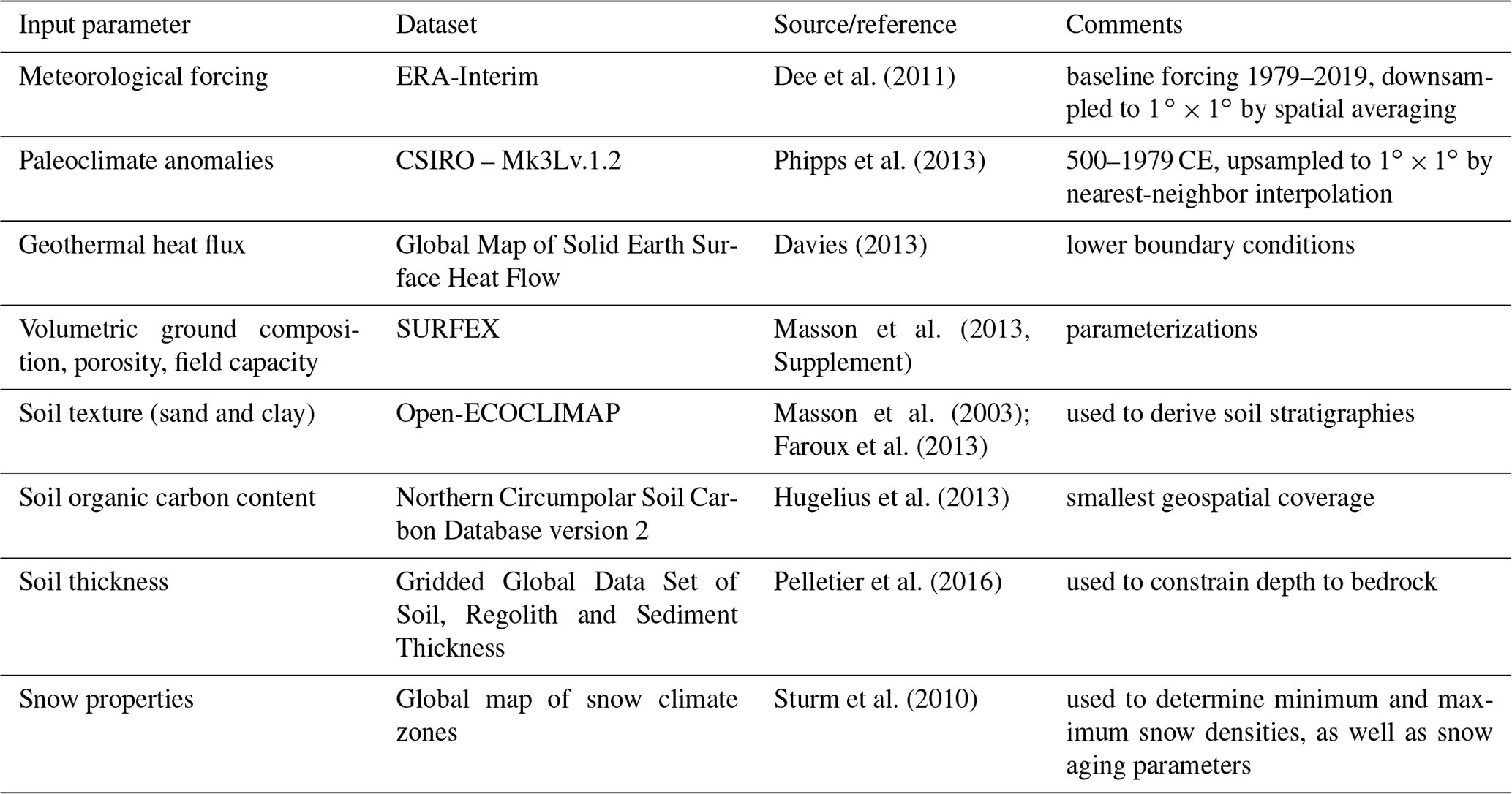
The model uses an external climate forcing of daily averages of surface temperature and precipitation. This greatly simplifies its application to very long time series spanning centuries to millennia. We consider daily mean near-surface air temperatures to be appropriate first-order estimates of surface temperatures. The snowfall is estimated from total precipitation that falls when air temperatures are below 0 ^∘C. The applied climate forcing consists of a synthesized time series of daily mean surface air temperatures and total precipitation combining paleoclimate simulations (500–1979 CE) and reanalysis data (1979–2019). We use paleoclimate simulations from the Commonwealth Scientific and Industrial Research Organisation (CSIRO) based on the Climate System Model Mk3Lv.1.2 from which we selected the ensemble including orbital, greenhouse gas, solar, and volcanic (OGSV) forcing due to its improved capability to reproduce climate reconstructions for the Northern Hemisphere and the inclusion of climate events such as volcanic eruptions (Phipps et al., 2013). From the OGSV ensemble we arbitrarily select an ensemble member (which differ only in initial conditions) to generate the forcing for our simulations. For the reanalysis period we applied ERA-Interim data (Dee et al., 2011). The paleo-simulations were harmonized with the ERA-Interim baseline data by applying decadal mean monthly anomalies of temperature and precipitation to the first decade (1980–1990) of the reanalysis data. The forcing at the lower boundary of the ground domain in 550 m depth is determined by a local geothermal heat flux according to the Global Map of Solid Earth Surface Heat Flow (Davies, 2013). The spatial resolution of the synthesized climate forcing data was set to 1 ^∘C, demanding spatial harmonization of the different forcing data. We applied spatial averaging for the ERA-Interim data (with nominal resolution of ≈80 km) and nearest-neighbor interpolation for CSIRO-Mk3Lv.1.2 (with nominal resolution of 5.68^∘ for longitude and 3.28^∘ for latitude) as well as for the geothermal heat flux map (with a nominal resolution of 2^∘). An overview of the input data used for model forcing and model parameterization is provided in Table 2.

Dee et al. (2011)Phipps et al. (2013)Davies (2013)Masson et al. (2013, Supplement)Masson et al. (2003); Faroux et al. (2013)Hugelius et al. (2013)Pelletier et al. (2016)Sturm et al. (2010)

Table 2 Overview of datasets used to force and parameterize CryoGridLite.

2.5 Diagnostics

For the model evaluation and analysis of the evolution of permafrost over the last 3 centuries, we apply different key diagnostics representing the thermal state of permafrost and the active layer. For the ground temperatures, we focus on the mean annual ground temperature in a depth of 10 m (MAGT_10 m), but we take additional depths into account for the sites at which we compare our model results with borehole measurements. To assess the state and changes in the active layer, we diagnose the maximum annual thawed ground depth [m] within the upper 10 m of the subsurface (TD_10 m), which corresponds to the active layer thickness (ALT) under stable permafrost conditions.

To assess the circumpolar extent of near-surface permafrost, we establish two criteria to distinguish the presence or absence of permafrost for a given year and ensemble member. Near-surface permafrost is defined to be absent if the thawed ground depth exceeds 3 m. Note that this criterion does not exclude the presence of permafrost, particularly in depths exceeding 3 m. The corresponding probability of near-surface permafrost occurrence is defined as the fraction of ensemble members where the criterion for absence is not fulfilled.

$$\begin{array}{}\text{(18)}& {\displaystyle }{p}_{\mathrm{3}\mathrm{m}}={\displaystyle \frac{\mathrm{1}}{n_{\text{ens}}}}\sum _{i=\mathrm{1}}^{n_{\text{ens}}}\left\{\begin{array}{l}\mathrm{0}\text{if}{\text{TD}}_{\mathrm{10}\mathrm{m}}^i>\mathrm{3}\text{m}\\ \mathrm{1}\text{else}\end{array}\right.\end{array}$$

Similarly, we diagnose the occurrence probability of permafrost within the upper 10 m of the subsurface as the fraction of ensemble members where some ground within the upper 10 m is frozen throughout the entire year.

$$\begin{array}{}\text{(19)}& {\displaystyle }{p}_{\mathrm{10}\mathrm{m}}={\displaystyle \frac{\mathrm{1}}{n_{\text{ens}}}}\sum _{i=\mathrm{1}}^{n_{\text{ens}}}\left\{\begin{array}{l}\mathrm{0}\text{if}{\text{TD}}_{\mathrm{10}\mathrm{m}}^i=\mathrm{10}\text{m}\\ \mathrm{1}\text{else}\end{array}\right.\end{array}$$

We note that the presence of permafrost according to our diagnostics based on the thawed ground depth also implies the fulfillment of the definition of permafrost-based maximum annual ground temperature. However, we only consider individual simulation years instead of 2 consecutive years (as required by the formal definition) and do not diagnose permafrost presence beyond 10 m depth. Combined, the applied diagnostics provide a nuanced insight into the dynamic evolution of permafrost conditions over a deeper volume in response to short- and long-term climatic changes. While the first criterion is often used in global-scale modeling to examine the impacts of climate warming on the permafrost carbon pool (e.g., Lawrence et al., 2008), the second criterion allows for the consideration of perennially frozen ground layers down to a depth of 10 m.

3 Results and discussion

3.1 Model evaluation

3.1.1 Ground temperatures

The ability of the model to reproduce the ground thermal regime and temperature trends in the Arctic permafrost region is evaluated using borehole temperature measurements from the Global Terrestrial Network for Permafrost (GTN-P) (Biskaborn et al., 2019). The dataset comprises n_GTNP=82 boreholes within our model domain which are located within n=47 different grid cells and for which it provides observations of mean annual ground temperatures (MAGTs) for the period from 2007 to 2016. For the model–observation comparison, the model output is compared at the depth closest to the measurement depth.

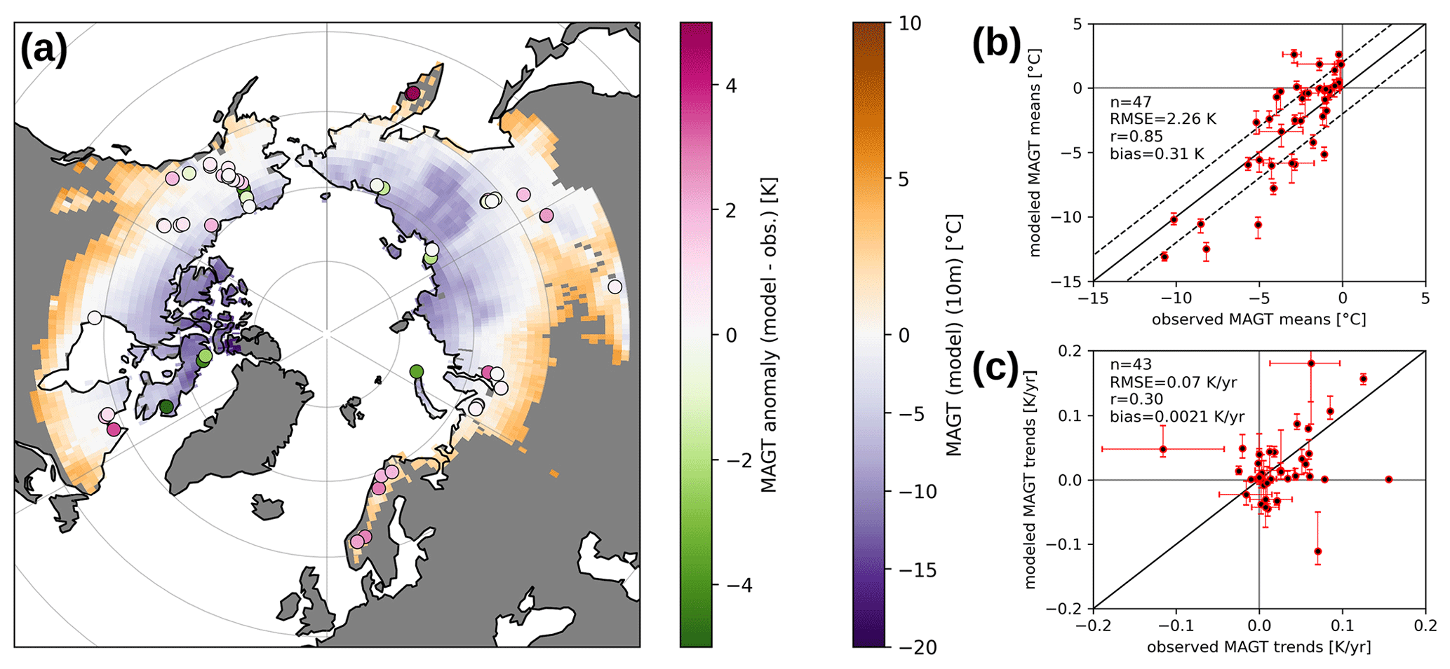
Figure 2 Map (a) showing modeled mean annual ground temperatures at 10 m depth (MAGT_10 m) averaged over the decade from 2007 to 2016. Circles indicate temperature deviations between the observed ground temperatures of the Global Terrestrial Network for Permafrost (GTN-P) boreholes and the modeled temperatures at the depth of the subsurface grid closest to the depth of the respective observations. Scatter plot (b) illustrating the agreement between observed and modeled MAGT (2007–2016 averages) with observations lying in the same model grid cell being grouped together. On the y axis the dots show the mean of the parameter ensemble, while the whiskers show the range between the 5th and 95th percentiles. Scatter plot (c) illustrating the agreement between observed and modeled (ensemble-mean) trends in MAGT, each derived from a linear least-squares regression over the 2007–2016 period. Observed trends are only included if there are 5 or more years of observations available. Horizontal error bars indicate the range of all observed trends belonging to the same model grid cell. Vertical error bars correspond to the 5th and 95th percentiles of the trends estimated by the parameter ensemble.

The comparison between observed and modeled average ground temperatures shows that at most sites (61.7 %) observed MAGT can be reproduced with deviations of up to ±2 K (Fig. 2a), in particular when the model range resulting from the parameter ensemble is considered. However, we note that this relatively good agreement between observations and model is partly due to a number of boreholes showing temperatures at or near 0 ^∘C (Fig. 2b). Because of the phase change of the ground ice and its stabilizing effect on the thermal conditions in the soil, temperatures around the freezing point are relatively easy to reproduce with the model. Overall, comparison between simulated and observed MAGT gives a root mean square error (RMSE) of 2.26 K and a slight warm bias of +0.31 K (Fig. 2b). The agreement with the borehole temperatures is comparable to or better than reported in previous modeling studies with a similar simulation domain (e.g., Ekici et al., 2014; Willeit and Ganopolski, 2015; Obu et al., 2019). Despite general agreement between observed and modeled ground temperatures, we emphasize that at single locations the model predicts positive MAGT, while the observations suggest permafrost to be present (Fig. 2b). The analysis further reveals some clear regional differences (Fig. 2a). In lowland permafrost regions (elevation ≤500 m, n=59), the simulated ground temperatures differ less from borehole measurements (RMSE=1.74 K, and $\mathrm{bias}=+\mathrm{0.17}$ K) than in mountainous terrain (elevation>500 m, n=23) where the deviations are larger (RMSE=3.10 K) and show a clear warm bias ($\mathrm{bias}=+\mathrm{1.65}$ K). This temperature bias is likely due to the coarse spatial resolution (1^∘) of the climate forcing data used. Variations in orography are averaged through the coarse grid resolution so that topographic climate effects are not accounted for. Since boreholes in mountainous regions are often located in higher terrain where permafrost occurs (e.g., in Norway), a warm bias is to be expected in a direct comparison.

At most borehole sites, the observed temperature trends can also be reproduced in sign and magnitude by the simulations (Fig. 2c). Here, the confidence intervals of the observed trends and the range of the simulated trends must be taken into account. Both ranges indicate relatively large uncertainties in temperature trends, in particular at sites showing relatively strong trends (absolute trend values >0.1 K yr⁻¹). On average the simulated trends show an RMSE of 0.07 K yr⁻¹. Nevertheless, the comparison between observed and measured temperature trends suggests that the model tends to underestimate observed warming.

A more detailed model evaluation is conducted for selected sites across the Arctic where long-term borehole measurements spanning periods of more than 10 years were available (see Appendix D). Overall, the simulated long-term ground temperature evolution is in agreement with observations, and remaining deviations can be explained by either inadequate forcing data or shortcomings in the model to reflect local environmental conditions.

3.1.2 Active layer thickness

We evaluate the capability of the model to reproduce the active layer thickness (ALT), i.e., the depth of the permafrost table, using field observations of the Circumpolar Active Layer Monitoring (CALM) program (Shiklomanov et al., 2012). The dataset comprises a total of n_CALM=166 sites within the simulation domain which are located in n=94 different model grid cells. Note that we compared the observed ALTs to the maximum annual thawed ground depth (TD_10 m) diagnosed from the simulations, which we subsequently denote as “modeled ALT” for simplicity.

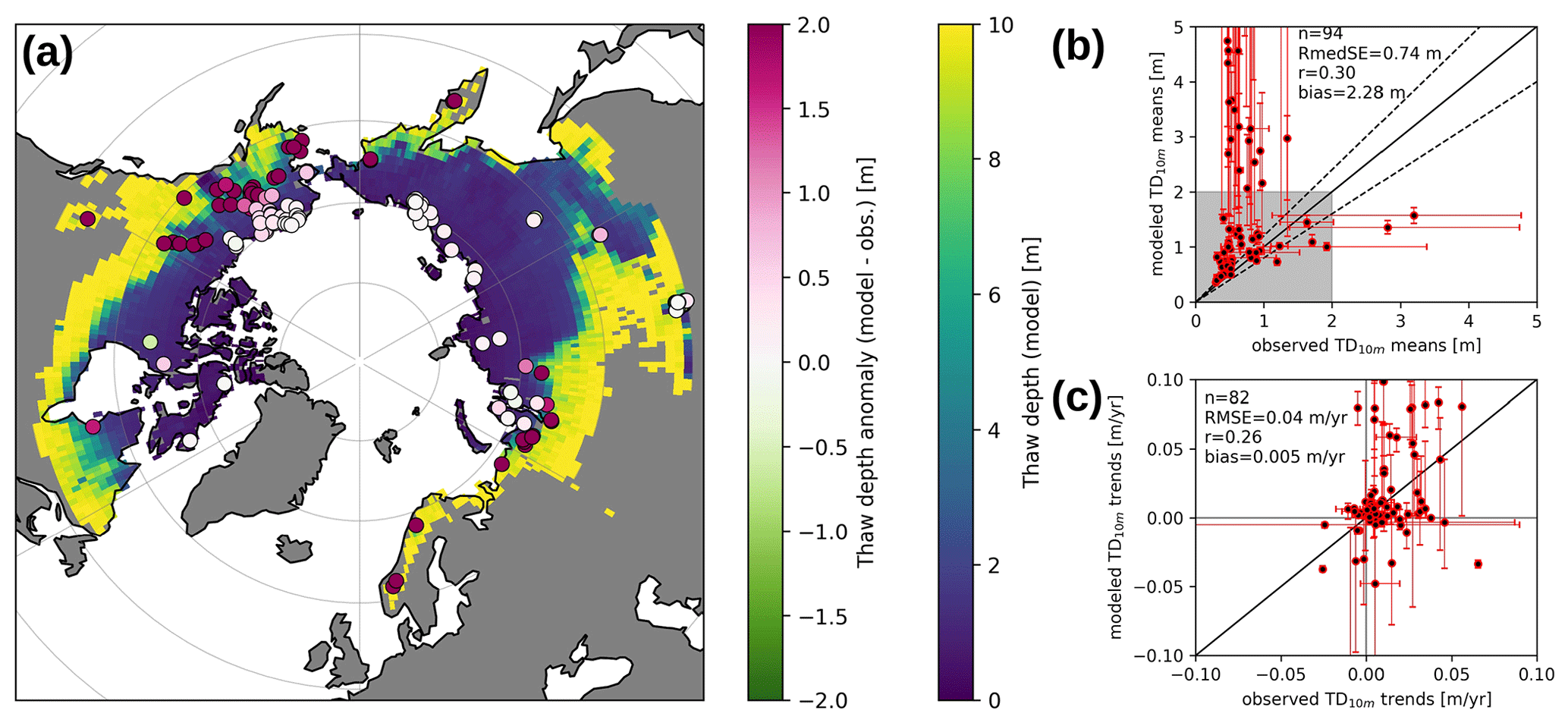
Figure 3 Map (a) showing the simulated maximum annual thaw depth (active layer thickness, ALT) averaged over the decade from 2007 to 2016. Circles indicate deviations between the ALT measurements of the Circumpolar Active Layer Monitoring (CALM) program and the modeled ALTs. Scatter plot (b) comparing CALM measurements and modeled ALTs (2007–2016 averages). On the y axis the dots indicate the mean of the model ensemble, with error bars indicating the range between the 5th and 95th percentiles. On the x axis the dots indicate the mean observed ALT thickness averaging all sites located within the corresponding model grid cell, and the error bars show the range of observations if there is more than one observation in the corresponding grid cell. Dashed lines indicate relative deviations of ±20 %, and the gray square indicates ALTs <2 m for which a comparison between measurements and simulations is most meaningful. Scatter plot (c) showing modeled and measured trends in ALT over the 2007–2016 period for all sites with observations available for 5 or more years. Vertical error bars correspond to the 5th and 95th percentiles of the simulated ALT trends, and horizontal error bars indicate the range of observed trends for grid cells with more than one corresponding measurement site.

Relatively small deviations (<0.1 m) between observed and modeled ALTs are found in the northern permafrost regions with small ALTs (<1 m) (Fig. 3a). In contrast, large deviations between modeled and observed ALTs (exceeding 2 m) are found for southern permafrost regions except for a few locations in the South Siberian Mountains. On average, the model is found to overestimate the ALTs in comparison to the CALM observations, resulting in a high root median squared error (RmedSE=0.74 m). However, considering the full range of the modeled parameter ensemble (Fig. 3b) reveals a high sensitivity of modeled ALTs to the simulated parameter range. In particular, locations with modeled average ALTs beyond 2 m reveal very broad ensemble ranges spanning several meters. At a few CALM sites, the model underestimates ALT; however, measurements within the same model grid cell at these sites show very high variability. Given the wide range of simulated ALTs among the members of the parameter ensemble and the fact that CALM sites are specific point observations rather than representative regional averages, it is found that the model at least partially reproduces observed ALTs realistically.

The comparison between modeled and observed ALT trends shows a large scatter (RSME=0.04 m yr⁻¹ with maximum values of about 0.10 m yr⁻¹) (Fig. 3c). However, the magnitude and sign of ALT trends are captured by the model, especially when uncertainties in the parameters are considered. The wide ranges of the ensemble simulations reveal a high sensitivity of the ALT trends to the groundwater and ground ice contents. On average, the model has a tendency to overestimate ALT changes for both ALT growth and ALT shrinkage using the current parameter ranges.

Several factors have to be considered for explaining the deviations between measured and modeled ALTs. First, at sites with deep active layers, ALT measurements with poke probes are often biased towards values that are too low, as gravel or other compact soil material can be misinterpreted as permafrost. Second, in southern areas, CALM sites are preferentially located at known permafrost sites such as peatlands, which are not representative of the large-scale picture. Third, our model does not fully take into account the protective effect of tall and dense vegetation cover, which would lead to shallower ALTs, especially in the boreal biome (e.g., Fisher et al., 2016; Stuenzi et al., 2022). Fourth, our model does not simulate thaw subsidence and soil compaction processes, which would reduce ALTs, especially in ice-rich regions (e.g., Günther et al., 2015; Nyland et al., 2021). Therefore, perfect agreement between modeled and observed ALTs on a circum-Arctic scale is not expected. Nevertheless, the simulation demonstrates the high sensitivity of the simulated ALT to local groundwater and ground ice contents, which are subject to large uncertainties and strong spatial variability. While the parameter ensemble simulations can provide insights into the associated model uncertainties, the actual spatial variability of groundwater and ice content remains an unresolved challenge.

3.2 Spatial and temporal evolution of permafrost temperatures

We evaluate the changes in the thermal state of permafrost based on mean annual ground temperatures in 10 m depth (MAGT_10 m) over 3 centuries from 1750 until 2000. We use the late 19th century (L19C) period (1850–1900) as the reference, based on which temperature anomalies are calculated for a previous period (1750–1800) representing the later 18th century (L18C) and a subsequent period (1950–2000) representing the more recent late 20th century (L20C) climate. The calculated MAGT_10 m values refer to temporal averages of the ensemble mean.

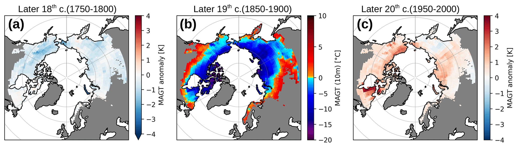
Figure 4 Map (a) showing the simulated anomaly of the mean annual ground temperatures in 10 m depth (MAGT_10 m) during the later 18th century (L18C, 1750–1800) relative to the L19C period (1850–1900) shown in (b). Map (c) showing the MAGT_10 m anomaly of the L20C climate period (1950–2000) relative to MAGT_10 m during the L19C period.

The MAGT_10 m anomalies show that the entire Arctic permafrost region is about 0.51 K colder during the later 18th century (L18C) compared to the L19C period (Fig. 4a). The permafrost on the North American continent (defined as 190–310^∘ E) is on average 0.57 K colder during the L18C with the strongest MAGT_10 m anomalies found in north-central Alaska, which is found to be more than 1 K colder during the L18C than during the L19C period. Temperature reconstructions based on tree-ring analyses show a distinct warm period for central Alaska between 1850 and 1900 (Barber et al., 2004), while lake sediment analyses suggest a distinct cold and dry period within the L18C period for the Alaskan Brooks Range (Bird et al., 2009). Cold air temperatures and low snow depths due to low precipitation explain the cold permafrost temperatures between 1750 and 1800 in north-central Alaska in our simulations. On the Eurasian continent, the differences in the MAGT_10 m between the L18C and L19C periods are found to be slightly smaller. The permafrost in eastern Siberia (defined as 120–190^∘ E) is found to be 0.55 K colder, and in western Siberia (60–120^∘ E) the simulated difference between the L18C and L19C periods is on average only −0.42 K. It is also worth noting that the L18C period coincides with the later part of the Little Ice Age, a generally colder period starting in the 13th century that affected large areas of the Northern Hemisphere (Miller et al., 2012). Thus, the significantly lower permafrost temperatures found here are also partly a legacy of this period of persistently cold climatic conditions which predate the L18C period under study (Halsey et al., 1995).

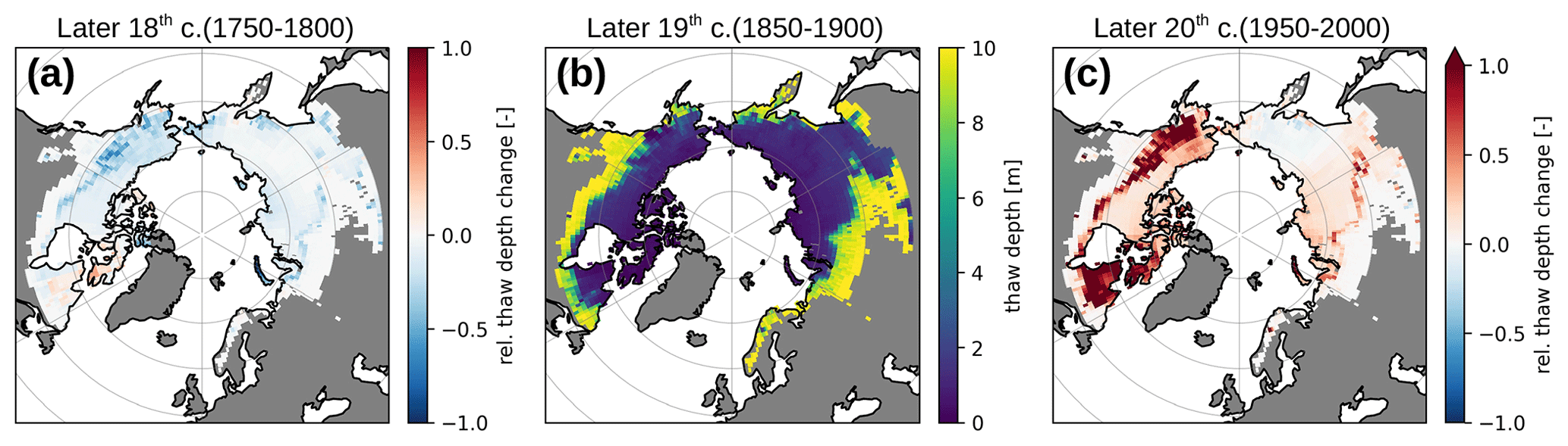
Figure 5 Map (a) showing the relative change in mean active layer thickness (ALT) between the later 18th century (1750–1800) and the L19C period (1850–1900). Map (b) showing the mean ALT during L19C period. Map (c) showing the relative change in mean ALT between the L20C (1950–2000) and the L19C period.

Between the L19C and L20C climate periods, the simulations reveal a general warming of the Arctic permafrost (+0.72 K, Fig. 4c). Three relative “hotspot” regions with MAGT_10 m anomalies above 1 K can be identified in northeastern Canada (Québec: 280–310^∘ E), northern Alaska (North Slope), and western Siberia. The region in Québec shows the strongest MAGT_10 m anomaly, indicating an average warming of 1.40 K between the L19C and L20C periods. At some grid cells the warming exceeds 3 K. This pronounced regional permafrost warming in our simulations is attributed to a warming of air temperature between 1970 and 1990 and to a shift in the seasonal snowfall distribution with earlier and heavier snowfall in autumn (October–November). For the Québec region observations and model results agree well for the L20C period (Fig. D1a, b). However, we note that the forcing data before 1980 are significantly colder than those after 1980. This temperature shift is attributed to the applied paleo-temperature anomaly. In particular, the cooling trend reconstructed by Chouinard et al. (2007) for the decades between 1950 and 1980 is not clearly visible in our forcing data. Also, regional differences such as the earlier ending of this cooling event in the eastern Canadian Arctic (e.g., Taylor et al., 2006) are not reproduced by our forcing data. Nevertheless, the modeled temperature anomalies (Fig. 4) indicate that the L20C period is much warmer than the L19C period. This finding is consistent with the observations and supported by the regional climate reconstruction in Chouinard et al. (2007), revealing a longer-term warming trend in northern Québec starting in the 18th century. On the North Slope the MAGT_10 m has also increased by more than 2 K, while the hotspot of warming in western Siberia is much less pronounced but still more than 1 K over a larger region.

Our simulations reveal pronounced regional differences in the development of the ground thermal regime during the last 300 years. Atmospheric and oceanic circulation patterns controlling the seasonal distribution of air temperature and precipitation may be responsible for the regional differences found in the simulations. The seasonal interaction of temperature and snowfall and its strong impact on the thermal state of permafrost are well known (Smith et al., 2022), and variation in snow cover can counteract the changes in air temperature (Taylor et al., 2006). Our long-term simulations over the last 3 centuries reveal increased spatial heterogeneity in the change in ground temperatures at regional scales (compare Fig. 2a, c). Simulations suggest that during the late 20th century (1950–2000), permafrost warming is observed in three hotspot regions. However, depending on long-term changes in Arctic climate, regional shifts or the emergence of other hotspots may occur. The regional hotspot of Arctic warming is currently located over the Barents Sea driven by sea ice loss and changes to atmospheric circulation (Rantanen et al., 2022).

3.3 Spatial and temporal evolution of the active layer thickness

Similar to changes in the ground temperatures, we evaluate relative changes in mean active layer thickness (ALT) based on the same centennial periods used to evaluate MAGT_10 m anomalies. The simulations reveal low to moderate changes in ALT between the L18C and L19C periods (Fig. 5a). ALT changes on the order of 50 % are nevertheless simulated for a narrow band on the North American continent (Fig. 5b). The simulated ALTs during the L19C (Fig. 5b) show that the transition from ALTs less than 2 m to ALTs greater than 10 m is very sharp. In warmer permafrost, especially in regions with higher ground ice content, the temperature profile is isothermal and the permafrost is close to the freezing point down to depths of 10 m or more (e.g., Romanovsky et al., 2010; Smith et al., 2010). A small increase in MAGT under such conditions is sufficient to thaw deep soil layers, which explains the sharp increase in ALT. This narrow transition zone at the southern fringe of the permafrost region marks the zone of active permafrost degradation and thus indicates the southern boundary of stable near-surface permafrost. For the Eurasian continent, minor changes (< 15 %) in mean ALT are simulated between the L18C and L19C periods. Substantial ALT changes are, however, simulated between the L20C and L19C periods (Fig. 5c). The simulation show a substantial increase in ALT of more than 100 % in the narrow boundary zone of near-surface permafrost on the North American continent. In particular, northeastern Canada (Québec) and southwestern Alaska are affected. A lower but still substantial increase in ALT (25 % to 80 %) is simulated at the boundary of the near-surface permafrost on the Eurasian continent. The simulations thus show a much greater loss of near-surface permafrost on the North American continent than on the Eurasian continent over the past 250 years.

3.4 Temporal evolution of the permafrost extent

The parameter ensemble allows us to diagnose an occurrence probability of permafrost (Eqs. 18 and 19) which can be used to assess the evolution of near-surface permafrost extent if interpreted as an areal fraction underlain by permafrost. Similar to Obu et al. (2019) we further distinguish four groups of permafrost occurrence probability (p>0.9, $\mathrm{0.9}\ge p>\mathrm{0.5}$, $\mathrm{0.5}\ge p>\mathrm{0.1}$, p≤0.1). These are oriented at the permafrost zones (continuous, discontinuous, sporadic, and isolated), but we emphasize that our diagnostics do not exactly correspond to these typical zones of spatial permafrost occurrence probability.

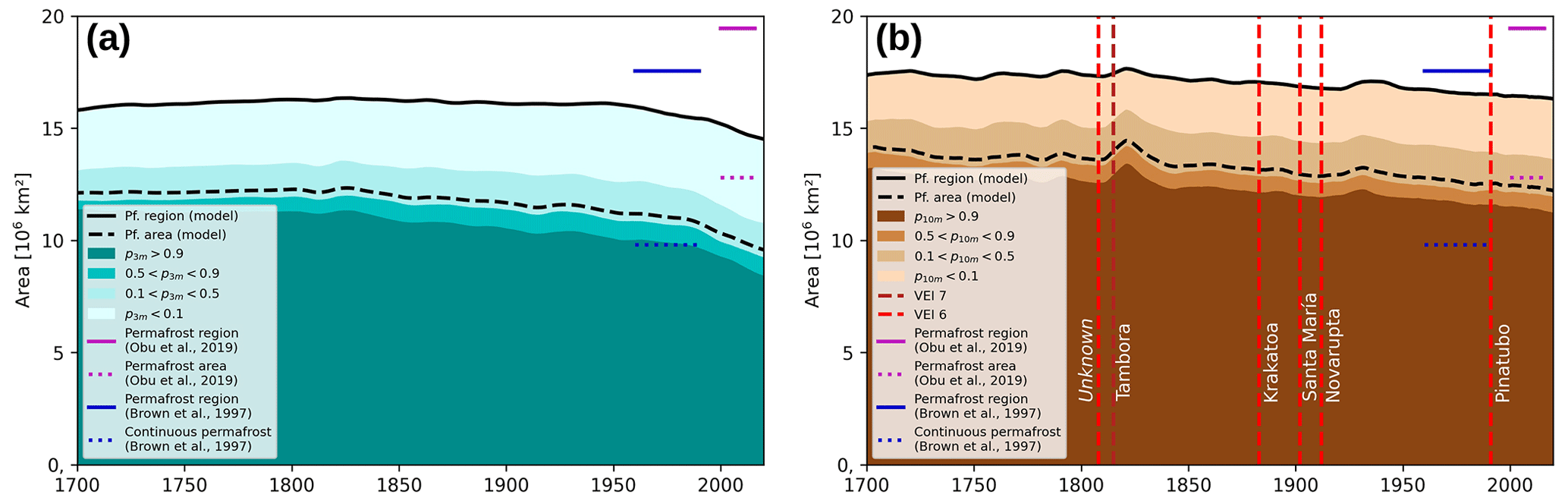
Figure 6 Areas of near-surface permafrost occurrence according to two different diagnostics focusing on (a) 3 m and (b) 10 m ground depth. The occurrence probabilities are derived from the parameter ensemble simulations and their grouping is aligned to the zonation of permafrost according to permafrost probability by Obu et al. (2019). Black lines indicate the simulated pan-Arctic area underlain by permafrost (dashed lines) and the area of the region where permafrost occurs (continuous lines). Horizontal lines mark the corresponding estimates as delineated by Brown et al. (1997) and Obu et al. (2019) for the late 20th and early 21st century, respectively. Dashed red vertical lines in (b) mark strong volcanic eruption events (volcanic eruption index – VEI, ≤6) which are represented in the applied climate forcing data.

Figure 6a shows the temporal evolution of the pan-Arctic area underlain by permafrost (dashed line) and of the area of the region where permafrost occurs (solid line) based on the probability p_3 m (Eq. 18; i.e., the probability of maximum annual thaw depths less than 3 m). The area underlain by permafrost (dashed line in Fig. 6a) is slightly decreased from its initial level of about 12×10⁶ km² during the 19th century, with a marked acceleration during the last 5 decades. It agrees well with the respective estimate by Brown et al. (1997) around the late 20th century. The area of the region where permafrost occurs (solid line in Fig. 6a) is almost constant at about 16×10⁶ km² from 1700 until it starts declining around the middle of the 20th century. It is, however, substantially smaller than the respective estimates by Brown et al. (1997) and Obu et al. (2019), which can be explained by the fact that the applied diagnostic does not capture permafrost conditions deep in the ground. In addition, the model likely underestimates the areas where permafrost is ecosystem-protected (see Appendix D, College Peat site; Fig. D1g).

The permafrost areal extents according to the p_10 m diagnostic (i.e., the probability of finding perennially frozen ground within the upper 10 m) provide a slightly different picture (Fig. 6b). These are generally higher than those according to the p_3 m diagnostic, since the occurrence of any perennially frozen layers within the upper 10 m is accounted for. Both the area underlain by permafrost (dashed line in Fig. 6b) and the area of the region where permafrost occurs (solid line in Fig.  6b) remain relatively stable throughout the 18th century before they start to decline during the 19th and 20th century. An acceleration of the decline towards the end of the analysis period as observed for the p_3 m diagnostic is not clearly visible. However, the p_10 m diagnostic is more sensitive to short-term climate fluctuations, therefore complementing the p_3 m diagnostic which responds faster to long-term climatic changes. The area of the region where permafrost occurs (solid line) for the late 20th century compares well with the estimate by Brown et al. (1997), while the area underlain by permafrost (dashed line) is about 3–4 million km² larger than the estimate by Brown et al. (1997). Combined with the insights from Fig. 6a, this suggests that the model ensemble likely underestimates the full extent of the transitional area where permafrost is not continuous.

3.4.1 Response of permafrost extent to climatic variability and change

We note that the beginning of the 19th century as well as the decades around the year 1900 experienced several large volcanic eruptions with impacts on the global climate (volcanic eruptions with VEI ≥6 during the analysis period: unknown, 1808/1809, see Guevara-Murua et al., 2014; Timmreck et al., 2021; Tambora, 1815; Krakatoa, 1883; Santa-Maria, 1902; Novarupta, 1912; Pinatubo, 1991). These climate events are included in the applied forcing data (Phipps et al., 2013) and their impact on permafrost extent can therefore be assessed. Our simulations suggest that the two tropical eruptions at the beginning of the 19th century (unknown and Tambora), as well as the Novarupta eruption in the Northern Hemisphere (Alaska), are associated with positive effects on the Arctic permafrost extent according to the p_10 m diagnostic (Fig. 6b). In particular, the zone of high permafrost occurrence probability is simulated to expand by several hundred thousand square kilometers after these events. However, these expansions only lasted for 2 to 3 decades before the zones began to decline again. Interestingly, these short-term increases in permafrost extent are not clearly visible if diagnosed using the p_3 m diagnostic (Fig. 6). This is explained by different sensitivities of the diagnostics to short-term variability and long-term changes in the climate, respectively.

The p_3 m diagnostic responds faster to the long-term warming during the 20th century since it is sufficient to thaw 3 m of permafrost within the upper 10 m of the ground for a location to be considered free of (near-surface) permafrost. Typically, thaw will also quickly affect deeper layers such that the thawed ground depth will be >3 m. A subsequent short-term cooling (e.g., due to a volcanic eruption) could lead to permafrost formation near the surface, but overall >3 m would remain thawed within the upper 10 m following the cooling event. Thus, the effect of volcanic eruptions is not visible in Fig. 6a, while the permafrost extent responds to the warming during the 20th century.

The p_10 m diagnostic only considers a location to be permafrost-free when the upper 10 m is completely thawed once within a year. Therefore, it does not respond so quickly to the long-term warming of the 20th century, as it takes time for permafrost sites to thaw completely down to a depth of 10 m. However, short-term cooling can lead to permafrost formation below the active layer, which would be directly diagnosed as permafrost according to this criterion.

Overall, the combination of the two diagnostics allows for nuanced insights into the response of permafrost conditions to short-term cooling and long-term warming of the climate.

3.5 Limitations and uncertainties

To keep CryoGridLite efficient enough to run a parameter ensemble simulation (n=50 per grid cell) for the Arctic permafrost region at a spatial resolution of 1^∘ and over a total time period of 1400 years, several simplifications and process exclusions are made. The model limitations and the resulting uncertainties in our simulations are summarized below.

• In this version of the model, ground freezing is approximated by an enthalpy–temperature relation of free water (see Appendix A). The implicit scheme used for CryoGridLite can theoretically be applied to arbitrary freezing characteristics, but convergence is not guaranteed and may require under-relaxation (Swaminathan and Voller, 1992). For the simulations and analyses performed, this means that an increase in thaw depth requires absorption of the total latent heat content as determined by the ice content. However, in fine-grained soils, the phase change may occur partially below the freezing point temperature so that in reality less latent heat is required to achieve an equal thaw depth. Consequently, there is a possibility of underestimation when evaluating simulated active layer thickness (ALT) for soils with high clay or silt content. Furthermore, any freezing point depressions (e.g., occurring in coastal regions due to salt) are not taken into account.

• The current model does not account for groundwater changes, so the total water–ice content for each ensemble member is assumed to be constant throughout the simulation period. Therefore, the model does not represent soil water fluxes. Thus, the effects of a climatically changing water balance on the permafrost temperatures are not captured by the simulations. However, uncertainties in soil water and ice contents are represented by the parameter ensemble simulations. The limitations imposed by a static hydrology are accepted to avoid the high computational cost of a full surface energy balance, which would require a model forcing that resolves the diurnal cycle and additional uncertain surface parameters.

• The probabilistic representation of soil and snow properties provides differentiated insight into the probability of permafrost occurrence. However, the ensemble of parameters used does not necessarily represent the actual local variability of surface and subsurface conditions. Due to lacking data on the probability distributions of the varied parameters, uniform distributions are used. Thus, permafrost occurrence is assessed by plausible parameter ranges, but the parameter ensemble does not necessarily correspond to the spatial permafrost occurrence probability. Furthermore, our simulations focus on the variability of groundwater and ice distributions, as well as highly variable snow cover properties. While our parameter ensemble approach was successful in reproducing MAGT variations due to variability in stratigraphy and snow height, it has limitations in accounting for mesoscale topographic effects. These effects are found to result in substantial temperature deviations between observations and simulations in mountainous and hilly terrain. Disregarding the variability of sub-grid topography thus potentially results in underestimating permafrost occurrence in mountain areas (Fiddes et al., 2019).

• The lack of representation of vegetation limits the model's ability to accurately simulate current permafrost conditions and to predict their long-term changes. Vegetation, like snow, plays an important role in regulating the surface temperature of the ground through its composition and structure. Vegetation acts as an insulating layer and affects the amount of solar radiation reaching the ground as well as the heat and moisture exchange with the atmosphere (e.g., Beringer et al., 2001; Stuenzi et al., 2022; Heijmans et al., 2022), and it modifies the snow cover. Neglecting the influence of vegetation leads to an underestimation of the extent of permafrost regions and their expansion to lower latitudes, where our current model tends to overestimate ALT values. Although vegetation is not explicitly represented, it is important to note that our model accounts for a range of isolating surface conditions. In this way, the parameter ensemble simulations performed partially emulate thermal buffer effects, such as those caused by organic surface layers, and provide an estimate of the potential probability of permafrost occurrence. However, we clarify the fact that ensemble simulations cannot capture the complex effects of dynamically evolving and responding vegetation cover, in particular in warm permafrost regions where permafrost occurrence is very sensitive to organic surface layer properties (James et al., 2013; Holloway and Lewkowicz, 2020). This could be problematic in accurately representing permafrost evolution in peatlands, particularly in the lowest-latitude regions where permafrost is reported to be an ecosystem-protected legacy of the Little Ice Age and earlier cold periods (Treat and Jones, 2018).

• The current scheme does not account for landscape change related to soil mechanical processes, such as ground subsidence due to pore ice and excess ice melt. Such thermokarst processes can greatly accelerate permafrost thaw regionally (Nitzbon et al., 2020). In addition, the warming effect of surface water such as ponds, lakes, and rivers (e.g., Langer et al., 2016; Juhls et al., 2021; Ohara et al., 2022) on the thermal state of the underlying and surrounding permafrost is also not considered, nor are their dynamic changes with time. Accounting for such non-gradual thaw processes would likely decrease the occurrence of near-surface permafrost, particularly in higher latitudes.

• Processes that stabilize or form permafrost due to, e.g., changes in surface water distribution (lakes and rivers), retreat of surface ice (glaciers and ice sheets), or post-glacial uplift in coastal regions are not taken into account.

Despite these limitations, we find that CryoGridLite provides a solid and efficient basis for realistically reproducing permafrost thermal dynamics at the pan-Arctic scale. Nevertheless, the identified shortcomings give rise to future model improvements. Operational parameterizations for local and regional permafrost models already exist for most of the processes not considered in the current model version (Nitzbon et al., 2019; Stuenzi et al., 2022; Westermann et al., 2023). Simplified and numerically optimized parameterizations can be derived from these and implemented in CryoGridLite. In particular, the ability of CryoGridLite to compute many instances of a grid cell allows the implementation of multi-tile approaches to represent sub-grid processes and their lateral interactions (Martin et al., 2021; Nitzbon et al., 2021).

4 Conclusions

In this study, an efficient numerical permafrost model is presented that bridges the gap between reduced-order permafrost schemes used in intermediate-complexity climate models and very detailed permafrost process models. The CryoGridLite model is tailored to enable parameter ensemble simulations of ground thermal dynamics covering the entire Arctic permafrost region and timescales beyond centuries. Despite limited process inclusion, the model is capable of estimating the thermal state of permafrost (RMSE=2.26 K) and its current warming rate. Taking into account possible biases caused by neglecting sub-grid variations in topography due to coarse spatial resolution of the climate data used, even higher accuracies are obtained (RMSE=1.74 K). The model is also able to provide a realistic estimate of active layer thickness (ALT), especially in the zone of continuous permafrost. Large uncertainties in ALT simulations are found in the zones of discontinuous to isolated permafrost and can likely be attributed to uncertain groundwater and ground ice contents as well as a lacking representation of vegetation cover.

The simulations performed show spatially heterogeneous warming of the permafrost during the last 250 years. Three hotspot regions characterized by particularly strong warming (>1 K) since industrialization (1900) were identified. Changes in ALT are simulated to occur mainly along the boundary between continuous and discontinuous permafrost. In particular, permafrost on the North American continent has been affected by a substantial increase in ALT (>100 %) since industrialization, whereas much smaller changes in ALT are simulated for the Eurasian Arctic permafrost. Generally, the North American continent is characterized by intense permafrost thaw, while Eurasian permafrost appears to have been less affected over the past 250 years.

The near-surface permafrost extent (i.e., permafrost within the upper 10 m below the surface) in the Arctic has changed significantly over the past 250 years. All Arctic permafrost zones combined have lost about 12 % of their area since 1850, with the most affected zone of continuous permafrost showing an area loss of about 20 %. A greatly accelerated decline in permafrost extent has occurred since the 1950s, with a loss of area of about $-\mathrm{1.36}\times \mathrm{105}$ km² decade⁻¹. It was found that climatic events caused by volcanic eruptions affect permafrost extent only for a very limited duration of a few decades.

Despite limited process representation compared to more complex permafrost process models, we conclude that CryoGridLite provides important insights into the long-term evolution of the thermal ground regime on the pan-Arctic scale. In particular, the model's ability to link multiple global datasets using a probabilistic ensemble approach allows CryoGridLite to deal with highly uncertain ground and snow properties. Future simulations could cover even larger timescales to investigate the formation of permafrost as a result of transient climate conditions from the Pleistocene to the present.

Appendix A: Details on the model formulation

Volumetric enthalpy, H_v, as a function of temperature, T, is defined as

$$\begin{array}{}\text{(A1)}& H_{\mathrm{v}}=T{C}_{\mathrm{v}}\left(T\right)+Lf\left(T\right),\end{array}$$

where C_v(T) [J m⁻³ K⁻¹] is the temperature-dependent volumetric heat capacity of the medium, L [J m⁻³] is the volumetric heat of fusion of water, and f(T) [m³ m⁻³] is the freezing characteristic curve which defines the relationship between temperature and volumetric liquid water content. The free water freezing characteristic defines the liquid fraction of water in terms of volumetric enthalpy:

$$\begin{array}{}\text{(A2)}& f_{\mathrm{wl}}\left(H_{\mathrm{v}}\right)=\left\{\begin{array}{ll}\mathit{\theta }& H_{\mathrm{v}}>L\mathit{\theta }\\ \frac{H_{\mathrm{v}}}{L}& \mathrm{0}\le H_{\mathrm{v}}\le L\mathit{\theta }\\ \mathrm{0}& H_{\mathrm{v}}<\mathrm{0},\end{array}\right.\end{array}$$

where θ is the total water content. Temperature can be determined via the corresponding inverse enthalpy function:

$$\begin{array}{}\text{(A3)}& H_{\mathrm{v}}^{-\mathrm{1}}\left(H_{\mathrm{v}}\right)=\left\{\begin{array}{ll}\frac{(H_{\mathrm{v}}-L\mathit{\theta })}{C_{\mathrm{v}}}& H_{\mathrm{v}}>L\mathit{\theta }\\ \mathrm{0}& \mathrm{0}\le H_{\mathrm{v}}\le L\mathit{\theta }\\ \frac{H_{\mathrm{v}}}{C_{\mathrm{v}}}& H_{\mathrm{v}}<\mathrm{0}.\end{array}\right.\end{array}$$

While the derivative of the enthalpy function $\frac{\mathrm{d}{H}_{\mathrm{v}}}{\mathrm{d}T}$ beyond the critical enthalpy range where a phase change occurs ($H_{\mathrm{v}}<\mathrm{0}\mathrm{or}{H}_{\mathrm{v}}>L\mathit{\theta }$) can simply be equated to C_v (see Eq. A1), within this range it would technically be infinite (see Eq. A2). In this case, a numerically convenient workaround is to simply set it to a very large value, e.g., $\frac{\mathrm{d}{H}_{\mathrm{v}}}{\mathrm{d}T}\approx \mathrm{1}\times {\mathrm{10}}^{\mathrm{9}}$ J m⁻³ K⁻¹.

Appendix B: Details on parameter values

Table B1 provides an overview of the thermal properties of the soil constituents that have been used to calculate the bulk properties using Eqs. (16) and (17).

Table B1 Overview of the heat capacity and thermal conductivity values used for the individual soil constituents. The values are based on Hillel (1998).

Appendix C: Numerical model accuracy and performance tests

We validate the numerical accuracy of the CryoGridLite implementation separately for the heat conduction problem (Fig. C1) and the phase change process (Fig. C2) using idealized test cases for which analytical solutions exist.

We furthermore compare the numerical performance of the integration scheme to other algorithms, revealing a very good performance in solving the heat conduction with phase change (Fig. C3).

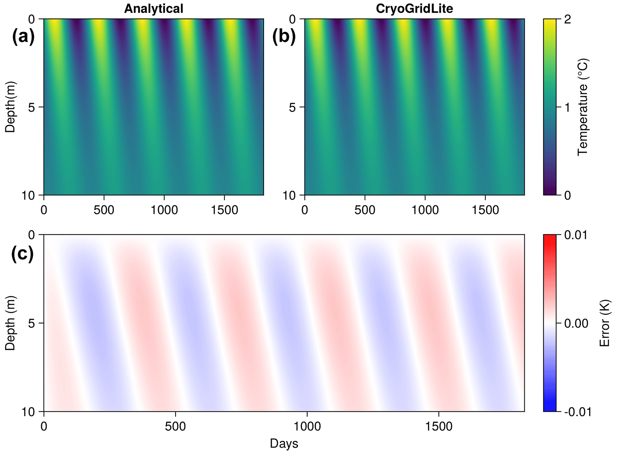
Figure C1 Evaluation of CryoGridLite in simulating heat diffusion with sinusoidal upper and zero flux lower boundary conditions without phase change. The analytical solution (a) for a semi-infinite half-space is compared to the solution obtained using CryoGridLite (b). Analysis of the differences (c) reveals a relatively small periodic error of less than ±0.01 K at deeper depths due to the spatial discretization. These results demonstrate that the numerical scheme effectively captures the heat diffusion process, yielding results that closely align with the analytical solution.

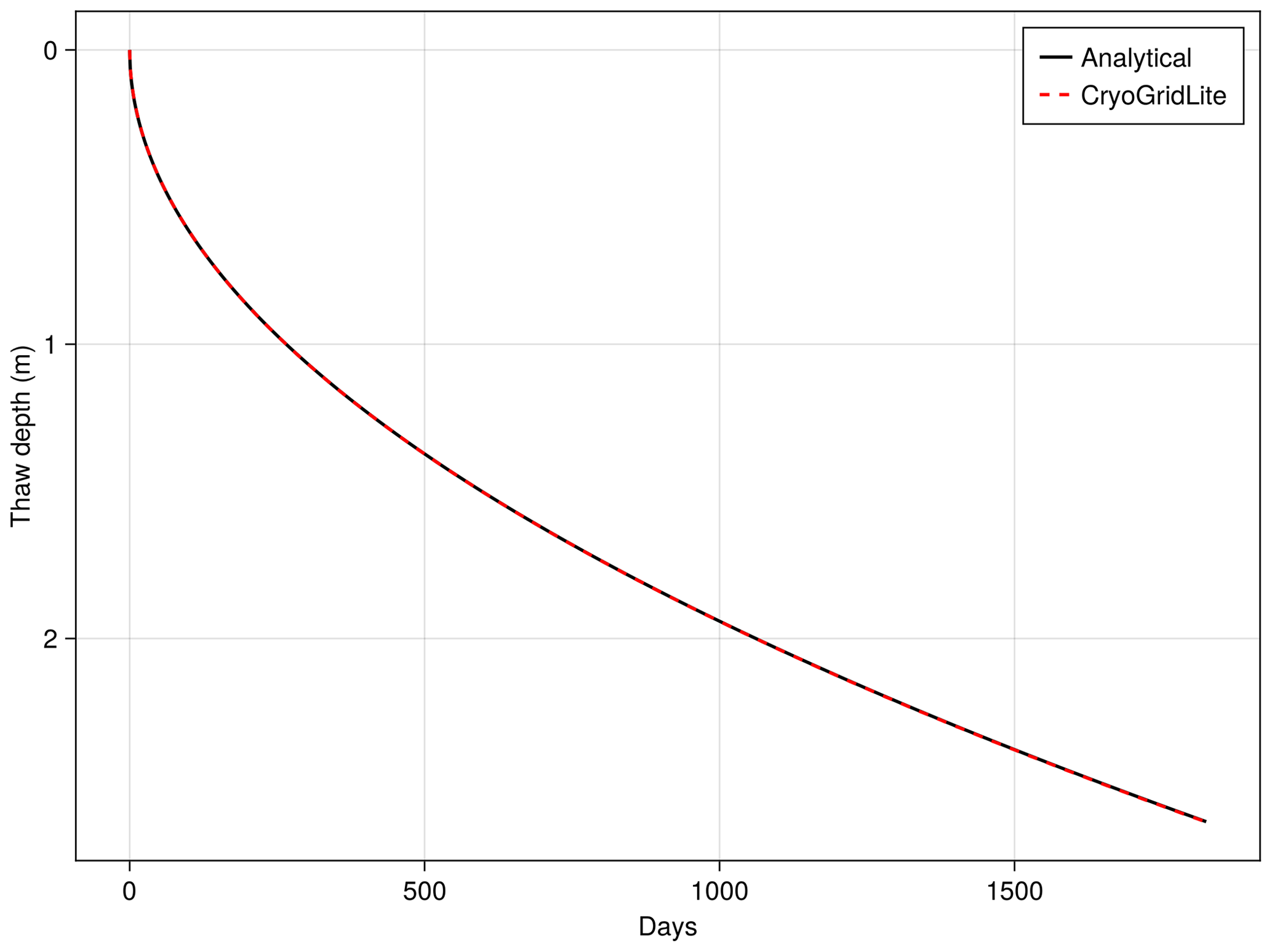
Figure C2 Comparison of the analytical solution to the two-phase Stefan problem and CryoGridLite for the one-sided thawing of a frozen soil column. The soil temperature is initialized at −0.02 ^∘C, and a constant upper boundary temperature of 1 ^∘C is applied for a period of 5 years. The spatial domain is discretized into a nonuniform rectangular grid cell with minimum spacing of 0.01 m down to a depth of 0.5 m. The good agreement between the analytical solution and the CryoGridLite simulation demonstrates that the model is able to accurately represent phase change of water.

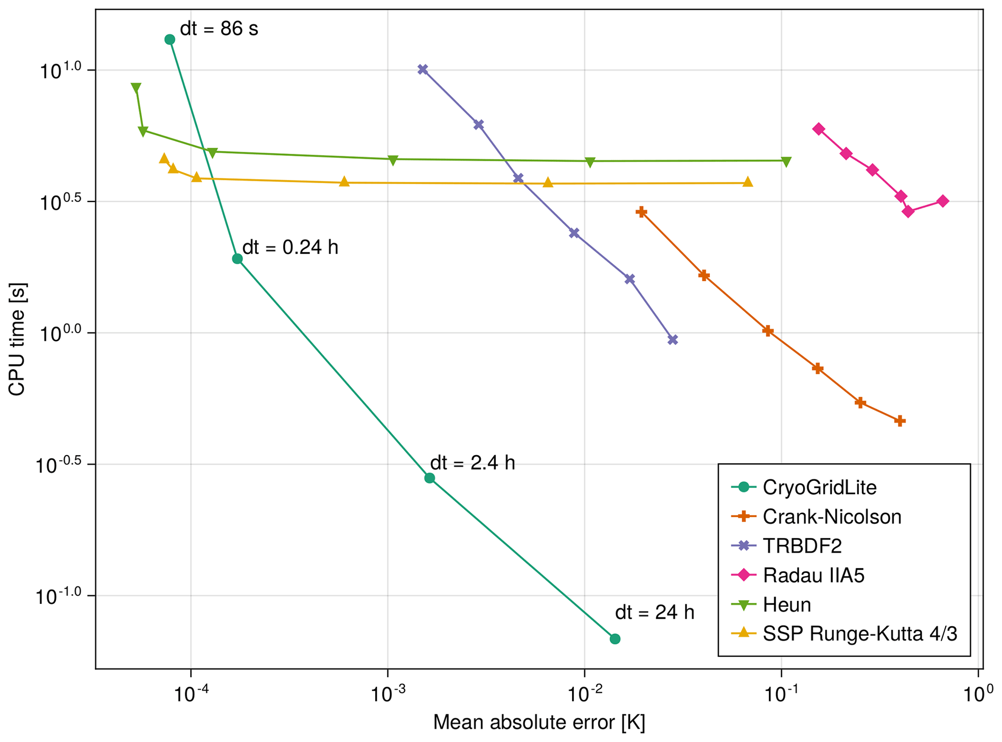
Figure C3 Work-precision plot comparing different numerical integration methods with CryoGridLite on heat conduction with phase change with a periodic upper boundary. The y axis shows the computational demand in CPU time of each numerical solve, while the x axis shows the global temperature error of the solution with respect to a high-resolution reference simulation using a 10-stage, fourth-order strong stability-preserving (SSP) Runge–Kutta with a 60 s time step. All of the algorithms (except CryoGridLite) use adaptive time stepping schemes with tolerances changed from 10⁻⁶ to 10⁻¹. Since CryoGridLite is a fixed-time-step method, we instead use a time step of 24 h scaled from 10⁻³ to 10⁰ for comparison. With the largest time step of 24 h CryoGridLite achieves an acceptable global error of approximately 0.014 K while being an order of magnitude more efficient than all other methods.

Appendix D: Evaluation of model simulations using borehole observations

In Fig. D1 we compare long-term ground temperature observations from 20 boreholes across Canada (five boreholes at three sites) (Allard et al., 2020), Russia (two boreholes at one site) (Smith et al., 2022), and Alaska (13 boreholes) to the corresponding model results from the closest grid cell within the model domain.

For the Canadian high Arctic site Alert on Ellesmere Island (Fig. D1a, b, c), the long-term observations from three boreholes agree reasonably well with the simulations, although a warming trend is more pronounced in the observations and the variability between the three boreholes is larger than the spread of the model ensemble. Here, the model ensemble likely underestimates the mesoscale variability in snow conditions (Smith et al., 2012). We further note that the closest model grid cell is located 5^∘ further south than the observation site.

For the Canadian sites in Québec (Quaqtaq and Salluit, Fig. D1d, e), the observed mean annual ground temperatures (MAGTs) at 10 m depth during the 2000s and 2010s are very well within the modeled ensemble range and even agree well with the model mean, especially for Quaqtaq, suggesting that the model ensemble captures site-level conditions. For a depth at 20 m, additional borehole observations are available for the late 1980s and early 1990s (Allard et al., 1995). The time series of measurements, however, is not long enough to confirm the pronounced negative temperature anomaly simulated before 1980 for Quaqtaq.

For the Alaskan sites, the agreement between the model and observations is also good, with some exceptions. For the relatively cold sites on the North Slope (from north to south: West Dock, Deadhorse, Franklin Bluffs, Happy Valley, Galbraith Lake; Fig. D1f, g, h, i, j), the observations are mostly within the range of the model ensemble. The observed long-term warming is underestimated in the simulations at the northernmost sites Deadhorse and West Dock, which might be explained by their proximity to the coast where the model forcing data might not be representative. The observed warming trend is well captured for the southern North Slope sites.

For the sites Chandalar Shelf and Coldfoot (Fig. D1k, l) which are located in the Brooks Range, the corresponding simulations are clearly too cold, which is likely attributable to the forcing data of the closest grid cell reflecting the colder North Slope climate.

At the interior sites in discontinuous permafrost (from north to south: Old Man, Livengood, College Peat, Birch Lake, Healy, Gulkana; Fig. D1m, n, o, p, q, r) the model simulates MAGTs at or just below 0 ^∘C, and the observations are mostly within the range of the ensemble. An exception is College Peat, where stable permafrost is observed in the borehole, but all simulations show temperatures to be in the zero curtain. Here, the insulating effect of the peat is not captured by the model ensemble.

The long-term measurements from borehole Urengoy 1 (Fig. D1s, t) in Russia show relatively cold borehole temperatures, and only the coldest simulations of the model ensemble show such low temperatures. Another borehole (Urgenoy 2) is located in the immediate vicinity but shows much warmer temperatures, which are within the model range.

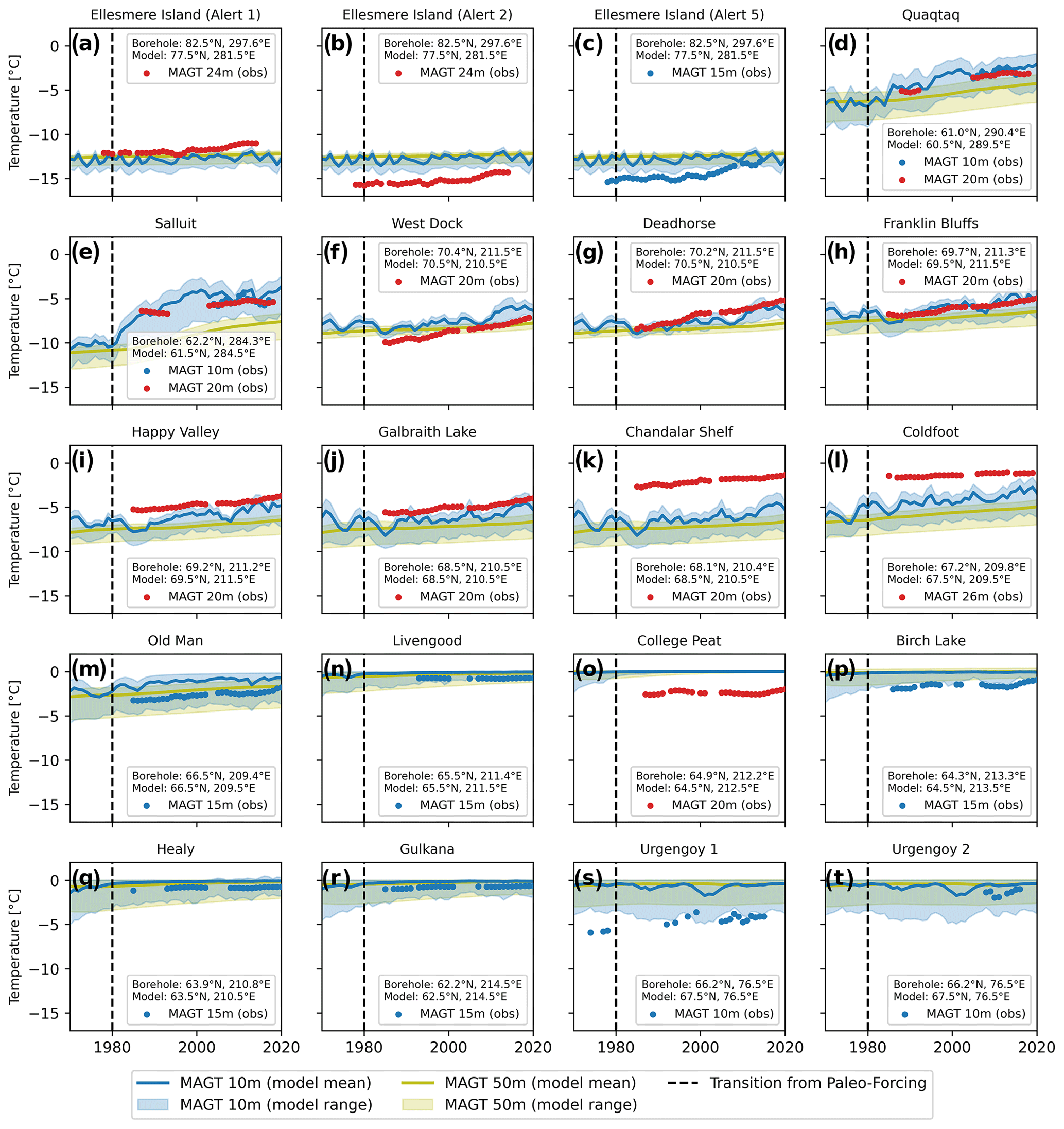
Figure D1 Model evaluation based on long-term ground temperature observations from 20 boreholes across Canada (5 boreholes), Russia (2 boreholes), and Alaska (13 boreholes).