Isotopic diffusion in ice enhanced by vein-water flow

Diffusive smoothing of signals on the water stable isotopes (¹⁸O and D) in ice sheets fundamentally limits the climatic information retrievable from these ice-core proxies. Past theories explained how, in polycrystalline ice below the firn, fast diffusion in the network of intergranular water veins “short-circuits” the slow diffusion within crystal grains to cause “excess diffusion”, enhancing the rate of signal smoothing above that implied by self-diffusion in ice monocrystals. But the controls of excess diffusion are far from fully understood. Here, modelling shows that water flow in the veins amplifies excess diffusion by altering the three-dimensional field of isotope concentration and isotope transfer between veins and crystals. The rate of signal smoothing depends not only on temperature, the vein and grain sizes, and signal wavelength, but also on vein-water flow velocity, which can increase the rate by 1 to 2 orders of magnitude. This modulation can significantly impact signal smoothing at ice-core sites in Greenland and Antarctica, as shown by simulations for the GRIP (Greenland Ice Core Project) and EPICA (European Project for Ice Coring in Antarctica) Dome C sites, which reveal sensitive modulation of their diffusion-length profiles when vein-flow velocities reach ∼ 10¹–10² m yr⁻¹. Velocities of this magnitude also produce the levels of excess diffusion inferred by previous studies for Holocene ice at GRIP and ice of Marine Isotope Stage 19 at EPICA Dome C. Thus, vein-flow-mediated excess diffusion may help explain the mismatch between modelled and spectrally derived diffusion lengths in other ice cores. We also show that excess diffusion biases the spectral estimation of diffusion lengths from isotopic signals (by making them dependent on signal wavelength) and the reconstruction of surface temperature from diffusion-length profiles (by increasing the ice contribution to diffusion length below the firn). Our findings caution against using the monocrystal isotopic diffusivity to represent the bulk-ice diffusivity. The need to predict the pattern of excess diffusion in ice cores calls for systematic study of isotope records for its occurrence and improved understanding of vein-scale hydrology in ice sheets.

1 Introduction

The water stable isotope records (δ¹⁸O, δD) from ice cores are key proxies for reconstructing palaeoclimatic temperature. Isotope diffusion, which occurs rapidly in firn (mainly by vapour diffusion in the pores) and slowly in ice below the firn transition, causes progressive smoothing that reduces the high-frequency content of these records, strongly attenuating the amplitude of short signals and limiting the depth to which annual and seasonal information survives (Johnsen, 1977; Whillans and Grootes, 1985; Cuffey and Steig, 1998; Johnsen et al., 2000). In the ice cores from central Greenland, annual signals often persist for ∼ 10⁴ years, to the early Holocene or just into the glacial part of the record (Johnsen, 1977; Johnsen et al., 1997, 2000), whereas in the ice cores from the East Antarctic plateau, they rarely penetrate through the firn into the ice, owing to low accumulation rates (causing short δ cycles, which decay quickly) and substantial noise and intermittency on the signals during deposition (Laepple et al., 2018; Casado et al., 2020).

Post-depositional diffusive smoothing limits the time resolution of real climate signals extractable from different depths of an ice-core isotope record. The smoothing rate needs to be known in several analyses: (i) studies that use “back diffusion” or deconvolution (Johnsen, 1977; Johnsen et al., 2000) to restore the original annual δ cycles at the surface, for inferring detailed climatic variations (e.g. Küttel et al., 2012; Zheng et al., 2018) or aiding the identification of annual layers in ice-core dating (e.g. Hammer et al., 1978; Vinther et al., 2006); (ii) studies that use the diffusion length σ estimated from the frequency spectrum of isotopic signals at different depths (including where annual cycles are no longer visible) to determine past changes in σ at the firn transition and hence reconstruct the surface temperature history by using the temperature dependence of firn isotope diffusion (e.g. Gkinis et al., 2014; Holme et al., 2018; Kahle et al., 2021); and (iii) studies that model the down-core profile of the diffusion length to assess the climatic variability on different timescales on a record (e.g. Jones et al., 2017; Gkinis et al., 2021; Grisart et al., 2022). The diffusion-length theory of Johnsen (1977), which tracks how σ evolves as a result of isotopic diffusion and vertical compression in the ice column, forms the basis of all these studies.

Whereas the smoothing process in firn has been studied sufficiently to yield models for temperature reconstructions (in (ii) above) and models able to reproduce the observed signal decay in firn (e.g. Cuffey and Steig, 1998; Johnsen et al., 2000; Gkinis et al., 2021), the smoothing process in ice remains poorly understood. We extend its theoretical description in this paper. Diffusive smoothing in ice can strongly impact deep isotopic signals given their long residence time; also, the diffusion rate increases in the warmer ice towards the ice-sheet base. Thus, a key concern motivating our work is that an inaccurate model for the signal smoothing rate in ice can bias the aforementioned studies – notably studies of types (ii) and (iii) above, when applied to records far under the firn transition. This problem may extend to reconstructions that use the differential diffusion length between oxygen and deuterium as a temperature proxy (Simonsen et al., 2011; Holme et al., 2018).

From the decay of annual δ¹⁸O cycles along the Holocene part of the GRIP (Greenland Ice Core Project) ice core, Johnsen et al. (1997) inferred an isotopic diffusion rate about 10 times faster¹ than the self-diffusion rate in ice monocrystals (Ramseier, 1967), measured at the temperature of the GRIP ice under analysis. They suggested the grain interfaces in polycrystalline ice as causing “excess diffusion” – an idea which prompted three mathematical models seeking to explain the phenomenon. Nye (1998) modelled the effect of water veins located at triple junctions of grain boundaries (Nye, 1989; Mader, 1992a, b) and showed how rapid (liquid phase) diffusion in the vein network “short-circuits” slow diffusion in the ice grains to enhance the signal decay rate above that due to solid diffusion. For signals at the decimetre scale, and ice with a mean grain size of several millimetres, his model predicts an enhancement that matches the GRIP observations. Johnsen et al. (2000) considered more generally interstitial water at grain boundaries as well as in the veins, and calculated how much these pathways raise the effective isotope diffusivity of the bulk ice. Their model couples the isotope concentrations in the solid and liquid in a less sophisticated way than Nye's treatment but accounts for the tortuosity of the veins, and they highlight the possibility for the acidity of the ice to affect the amount of interstitial water. Lastly, Rempel and Wettlaufer (2003), building upon Nye's (1998) continuum description of the grain–vein system, showed that the perfect short-circuiting assumed in Nye's model overestimates the excess diffusion: the enhancement is less than the value predicted by Nye since the liquid diffusivity is high but finite. Rempel and Wettlaufer (2003) clarified the two previous models as end-member approximations of the system, and like Nye's result, their solution gives the enhancement as a function of signal wavelength. All three models – of Nye, Johnsen et al., and Rempel and Wettlaufer – predict a higher enhancement for thicker veins, because wider liquid pathways promote short-circuiting.

Despite these models' implication that recrystallisation and impurity processes in polycrystalline ice can alter the amount of excess diffusion to shape the signals on isotope records in complex ways, no diffusion-length-based models or temperature reconstructions have yet incorporated their results into calculations, which often assume the monocrystal diffusivity of Ramseier (1967) below the firn transition. Nor has there been progress in unravelling the controls and mechanisms of excess diffusion – by theory or experiment – for 2 decades. Yet, the potential occurrence of excess diffusion continues to concern ice-core studies. When analysing the WAIS (West Antarctic Ice Sheet) Divide ice core, Jones et al. (2017) invoked excess diffusion as one of several explanations why diffusion lengths derived from δD signals at ≈ 15–18 ka BP exceeded modelled diffusion lengths based on Ramseier's diffusivity by up to 1.6 times. For the high-resolution δD record of the EPICA (European Project for Ice Coring in Antarctica) Dome C core, Pol et al. (2010) regarded vein-driven enhancement of isotopic diffusion to be the cause of strong smoothing and near absence of sub-millennial scale signals across Marine Isotope Stage 19 (MIS 19) – the oldest interglacial identified in that core, at ∼ 780 ka BP – where spectrally derived diffusion lengths (∼ 40 to 60 cm) are several times higher than predicted by the monocrystal diffusivity. Excess diffusion is expected to impact the preservation of deep isotopic signals in the ice cores to be retrieved at Little Dome C, Antarctica, by the European Beyond EPICA project and the Australian Million Year Ice Core project, which aim to obtain records reaching back ∼ 1–1.5 Ma and covering the Mid-Pleistocene Transition.

Herein, we revisit Nye's (1998) and Rempel and Wettlaufer's (2003) formulation for vein-mediated excess diffusion, asking “what if the vein water isn't stagnant, but percolates?” In our modelling in Sects. 2 and 3, we show that vein-water flow distorts the isotopic concentrations in ice grains and modifies their isotope exchange with the veins, so that excess diffusion acting on isotopic signals is always increased from the no-flow case. The mechanism causes signals to move relative to the ice, although the age offset of displaced signals is much less than their absolute age. Depending on the water flow velocity, the decay-rate enhancement for decimetre-scale signals can vary by a factor of several to a few hundred – between Rempel and Wettlaufer's and Nye's predictions. This modulation highlights the vein hydrology of ice sheets as a major knowledge gap. In Sect. 4 we explore its impact on signal smoothing at ice-core sites by embedding it in diffusion-length simulations for the GRIP and EPICA ice cores. We show that excess diffusion can undermine diffusion-based temperature reconstructions and the spectral derivation of diffusion lengths from isotope records. We conclude with broader perspectives in Sect. 5.

2 Mathematical model

As in Nye's (1998) and Rempel and Wettlaufer's (2003) studies, our modelling in this section focusses on the interactions between crystals and veins at the grain scale, ignoring the effect of ice deformation on isotopic signals and ignoring diffusion along grain boundaries. Vertical compression will be accounted for in Sect. 4. Background about the diffusion-length theory will be given there.

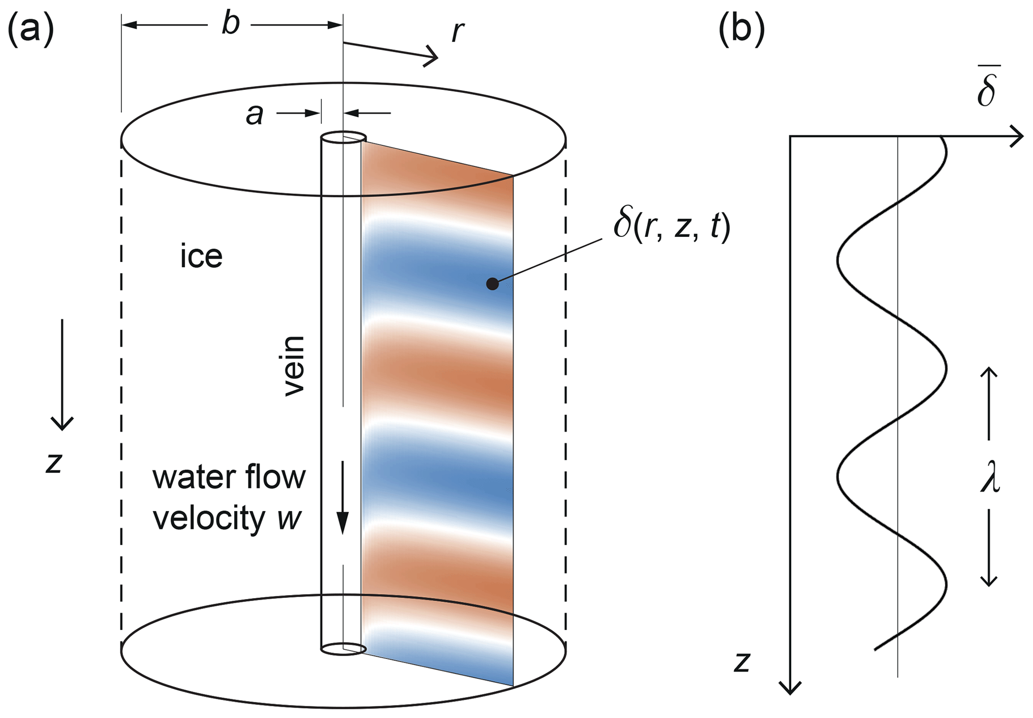
Figure 1 Model geometry and symbols. (a) Ice annular cylinder surrounding a vein. Colour image shows a radial cross-section of the isotopic deviation δ in the ice, exemplifying the signals studied in Figs. 3 to 5. The pattern is distorted by the boundary condition at the vein wall due to isotope advection by vein-water flow. (b) Depth profile of the mean isotopic signal.

First we extend their equations to incorporate vein-water flow. We adopt their idealised geometrical set-up (Fig. 1), which represents ice crystal grains as a vertical annular cylinder, with outer radius b, and the water vein as a hole at its centre, with the vein wall located at the inner radius, r=a ($\sim {\mathrm{10}}^{-\mathrm{6}}$ m); r is the radial coordinate. We distinguish the vein radius a from the radius of curvature of real (convex) vein walls (Nye, 1989; Mader, 1992a; Ng, 2021). In plan view, each cylinder is meant to approximate a unit cell of polycrystalline ice around a vein, so b is taken as the mean grain radius (∼ 10⁻³ m). As the original studies assumed, the vein water is kept liquid by a high concentration of dissolved ionic impurities, which lowers the eutectic temperature; horizontal (near-horizontal) veins are disregarded as they cause no (negligible) short-circuiting of depth-varying isotope signals. With the z coordinate axis pointing down, and t denoting time, the concentrations of a trace isotope (¹⁸O or D) in the ice grains and in the vein water – N_s(r, z, t) and N_v(z, t), respectively – satisfy the conservation equations

$$\begin{array}{}\text{(1)}& {\displaystyle \frac{\partial N_{\text{s}}}{\partial t}}=D_{\text{s}}\left({\displaystyle \frac{\mathrm{1}}{r}}{\displaystyle \frac{\partial }{\partial r}}\left(r{\displaystyle \frac{\partial N_{\text{s}}}{\partial r}}\right)+{\displaystyle \frac{{\partial }^{\mathrm{2}}{N}_{\text{s}}}{\partial z^{\mathrm{2}}}}\right),\text{(2)}& {\displaystyle \frac{\partial N_{\text{v}}}{\partial t}}=D_{\text{v}}{\displaystyle \frac{{\partial }^{\mathrm{2}}{N}_{\text{v}}}{\partial z^{\mathrm{2}}}}+{\displaystyle \frac{\mathrm{2}{D}_{\text{s}}}{a}}{\left.{\displaystyle \frac{\partial N_{\text{s}}}{\partial r}}\right|}_{r=a}-w{\displaystyle \frac{\partial N_{\text{v}}}{\partial z}},\end{array}$$

where D_s and D_v are molecular diffusivities in the solid (single crystal) and water. Following the original studies, N_v is assumed independent of r, and we specify $\partial N_{\mathrm{s}}/\partial r=\mathrm{0}$ at r=b as a boundary condition. In Eq. (2), which couples N_s and N_v, the D_s term represents isotope transfer between ice and vein. The final term – our addition to the model – describes advection of N_v by vein water flowing at velocity w (mean value across vein, defined positive downward).

Equilibrium fractionation at the ice–water interface implies $\mathit{\alpha }{N}_{\mathrm{v}}/N_{\mathrm{v}\mathrm{0}}=N_{\mathrm{s}}{|}_{r=a}/N_{\mathrm{s}\mathrm{0}}$, where α (≈ 1) is the fractionation coefficient, and N_v0 and N_s0 (assumed constant) are the number densities of the major isotope (¹⁶O or H) in water and ice. Following the procedure of Rempel and Wettlaufer (2003), we rewrite N_v in Eq. (2) in terms of $N_{\mathrm{s}}{|}_{r=a}$, assuming N_v0≈N_s0, and express N_s as the isotopic deviation $\mathit{\delta }=\mathit{\delta }(r,z,t)=N_{\mathrm{s}}/N_{\mathrm{s}\mathrm{0}}-\mathrm{1}$, thus deriving

$$\begin{array}{}\text{(3)}& {\displaystyle \frac{\partial \mathit{\delta }}{\partial t}}=D_{\text{s}}\left({\displaystyle \frac{\mathrm{1}}{r}}{\displaystyle \frac{\partial }{\partial r}}\left(r{\displaystyle \frac{\partial \mathit{\delta }}{\partial r}}\right)+{\displaystyle \frac{{\partial }^{\mathrm{2}}\mathit{\delta }}{\partial z^{\mathrm{2}}}}\right),\end{array}$$

with the boundary conditions

$$\begin{array}{}\text{(4)}& {\left.{\displaystyle \frac{\partial \mathit{\delta }}{\partial r}}\right|}_{r=b}=\mathrm{0}\end{array}$$

and

$$\begin{array}{}\text{(5)}& \begin{array}{rl}{\left.{\displaystyle \frac{{\partial }^{\mathrm{2}}\mathit{\delta }}{\partial r^{\mathrm{2}}}}\right|}_{r=a}& +{\displaystyle \frac{\mathrm{1}-\mathrm{2}\mathit{\alpha }}{a}}{\left.{\displaystyle \frac{\partial \mathit{\delta }}{\partial r}}\right|}_{r=a}-\mathit{\beta }{\left.{\displaystyle \frac{{\partial }^{\mathrm{2}}\mathit{\delta }}{\partial z^{\mathrm{2}}}}\right|}_{r=a}\\ & +{\displaystyle \frac{w}{D_{\text{s}}}}{\left.{\displaystyle \frac{\partial \mathit{\delta }}{\partial z}}\right|}_{r=a}=\mathrm{0}.\end{array}\end{array}$$

The second boundary condition has been derived by eliminating the time derivatives between Eqs. (1) and (2). The dimensionless parameter

$$\begin{array}{}\text{(6)}& \mathit{\beta }={\displaystyle \frac{D_{\text{v}}}{D_{\text{s}}}}-\mathrm{1}(>\mathrm{0})\end{array}$$

quantifies the diffusivity contrast of water to ice. The diffusivities D_s and D_v vary strongly with temperature T, and typically β∼10⁶ (Fig. 2). As detailed in Appendix A, we use Ramseier's (1967) formula for D_s(T), and for D_v(T) we use an extension of Gillen et al.'s (1972) formula that is valid down to −60 ^∘C.

Equations (3) to (5) form a partial differential equation model for $\mathit{\delta }(r,z,t)$. Rempel and Wettlaufer (2003) assumed 1–2$\mathit{\alpha }\approx -\mathrm{1}$ in Eq. (5), so their model is independent of the fractionation coefficient α and applies equally to δ¹⁸O and δD. This is a good approximation because α(¹⁸O $/$ ¹⁶O) ≈ 1.0029 and α(D $/$ H) ≈ 1.021 (Lehman and Siegenthaler, 1991; O'Neill, 1968; Árnason, 1969). We make the same approximation in most of Sects. 3 and 4, but not in the present derivation, as we need a general model that observes the precise value of α for an analysis about dual-isotope thermometry at the end of Sect. 4.

Equations (3) to (5) encapsulate the short-circuiting effect and differ from Rempel and Wettlaufer's (2003) model by the w term only. When studying the system without water flow (w=0), these authors explained that Nye's (1998) model corresponds to the limit β→∞, as it supposes liquid diffusion so fast that δ along the vein is constant (i.e. perfect short-circuiting); on the other hand, the model of Johnsen et al. (2000) effectively assumes instantaneous radial diffusion in the grains, so that longitudinal diffusion along the vein and in the ice governs the smoothing of signals. Hence, the Johnsen et al. model predicts an excess diffusion equal to Rempel and Wettlaufer's prediction for slow-varying (long) signals, but it is not strictly an approximation of our model at a limit of a defined parameter here. We shall not compare its predictions against our results.

When vein-water flow occurs (w≠0), we expect advection of δ at the vein boundary to perturb δ in the ice (Fig. 1), causing the isotopic signals there to move also. To study how signals behave, we seek a separable solution of the form

$$\begin{array}{}\text{(7)}& \mathit{\delta }(r,z,t)={\mathit{\delta }}_{\mathrm{0}}+{\mathit{\delta }}_{\mathrm{1}}F\left(r\right)\exp (-D_{\text{s}}\mathit{\zeta }t+i{k}_{z}z),\end{array}$$

where $\mathit{\zeta }={\mathit{\zeta }}_{\mathrm{R}}+i{\mathit{\zeta }}_{\mathrm{I}}$ is a decay-rate parameter for sinusoidal signals with the wavenumber k_z (or wavelength $\mathit{\lambda }=\mathrm{2}\mathit{\pi }/k_z$), and δ₀ and δ₁ are arbitrary constants representing the background level and amplitude of signals. The amplitude of signals decays at the rate D_sζ_R, whereas their “baseline” decay rate in ice without veins (due to solid diffusion alone) would be $D_{\mathrm{s}}{k}_z^{\mathrm{2}}$. Following Nye (1998) and Rempel and Wettlaufer (2003), we let

$$\begin{array}{}\text{(8)}& {\mathit{\zeta }}_{\text{R}}=k_z^{\mathrm{2}}+k_{\mathrm{r}}^{\mathrm{2}}=f{k}_z^{\mathrm{2}},\end{array}$$

in which the “enhancement factor”

$$\begin{array}{}\text{(9)}& f=\mathrm{1}+{\displaystyle \frac{k_{\mathrm{r}}^{\mathrm{2}}}{k_z^{\mathrm{2}}}}\end{array}$$

measures how much faster signals decay in the presence of veins, or equivalently, how much the veins increase the effective diffusivity of the system above D_s. Owing to their short-circuiting effect, excess diffusion operates (f>1) even when w=0. Our main interest is how f varies with w. Note that f, k_r, ζ_R, and ζ_I are functions of k_z.

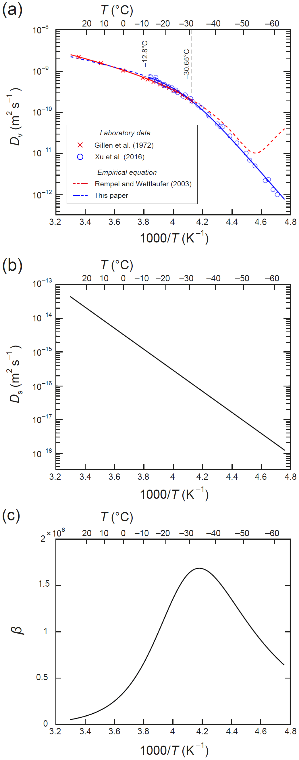
Figure 2 Isotopic diffusivities and their temperature dependence. (a) Arrhenius plot of the self-diffusivity of water D_v. Symbols plot values based on laboratory measurements. Blue curve: our composite exponential in Eq. (A1), fitted to the data of Xu et al. (2016) and used to calculate D_v in this paper. Red curve: quadratic fit by Rempel and Wettlaufer (2003) to the data of Gillen et al. (1972); the dashed portion evaluates their quadratic at T below −31 ^∘C, outside its region of applicability. (b) Self-diffusivity of monocrystalline ice D_s, calculated with Ramseier's (1967) empirical formula in Eq. (A2). (c) The liquid-to-solid diffusivity contrast β (= $D_{\mathrm{v}}/D_{\mathrm{s}}-\mathrm{1}$).

Hitherto we seem to be mostly retracing the steps of Nye (1998) and Rempel and Wettlaufer (2003). But a key difference herein – and what distinguishes our findings – is that the decay-rate parameter ζ and the amplitude function F in Eq. (7) are complex numbers when w≠0, since the problem is then no longer symmetric in z. Particularly, a non-zero ζ_I implies signal migration at the velocity $v={\mathit{\zeta }}_{\mathrm{I}}{D}_{\mathrm{s}}/k_z$, and we anticipate $F\left(r\right)=F_{\mathrm{R}}\left(r\right)+i{F}_{\mathrm{I}}\left(r\right)$, with the signal phase given by $\mathit{\theta }\left(r\right)={\tan }^{-\mathrm{1}}(F_{\mathrm{I}}/F_{\mathrm{R}}$), varying with radius under the advection. Symmetry considerations for how the system behaves when the vein-water flow direction is reversed predict ζ_R (hence f) and ζ_I (hence v) to be even and odd functions of w, respectively.

Now, substituting Eq. (7) into Eqs. (3), (4), and (5) leads to the Bessel equation

$$\begin{array}{}\text{(10)}& F^{\prime \prime }+{\displaystyle \frac{F^{\prime }}{r}}+(k_{\mathrm{r}}^{\mathrm{2}}+i{\mathit{\zeta }}_{\mathrm{I}})F=\mathrm{0},\end{array}$$

with the boundary conditions

$$\begin{array}{}\text{(11)}& {\displaystyle }{F}^{\prime }\left(b\right)=\mathrm{0},\text{(12)}& {\displaystyle }{F}^{\prime \prime }\left(a\right)+{\displaystyle \frac{\mathrm{1}-\mathrm{2}\mathit{\alpha }}{a}}{F}^{\prime }\left(a\right)+\left(\mathit{\beta }{k}_z^{\mathrm{2}}+{\displaystyle \frac{i{k}_{z}w}{D_{\text{s}}}}\right)F\left(a\right)=\mathrm{0}.\end{array}$$

Suppose $k_{\mathrm{r}}^{\mathrm{2}}+i{\mathit{\zeta }}_{\mathrm{I}}\equiv s^{\mathrm{2}}=(s_{\mathrm{R}}+i{s}_{\mathrm{I}}{)}^{\mathrm{2}}$, such that

$$\begin{array}{}\text{(13)}& k_{\mathrm{r}}^{\mathrm{2}}=s_{\mathrm{R}}^{\mathrm{2}}-s_{\mathrm{I}}^{\mathrm{2}}\text{and}{\mathit{\zeta }}_{\mathrm{I}}=\mathrm{2}{s}_{\mathrm{R}}{s}_{\mathrm{I}}.\end{array}$$

Then, in terms of Bessel functions, the analytic solution of Eqs. (10) to (12) is

$$\begin{array}{}\text{(14)}& F\left(r\right)=J_{\mathrm{0}}\left(sr\right)-{\displaystyle \frac{J_{\mathrm{1}}\left(sb\right)}{Y_{\mathrm{1}}\left(sb\right)}}{Y}_{\mathrm{0}}\left(sr\right)\end{array}$$

(or any constant multiples), in which s at each wavenumber k_z satisfies

$$\begin{array}{}\text{(15)}& \begin{array}{rl}& {\displaystyle \frac{\mathrm{2}\mathit{\alpha }s}{a\left[s^{\mathrm{2}}-\mathit{\beta }{k}_z^{\mathrm{2}}-i{k}_{z}w/D_{\text{s}}\right]}}\\ & -{\displaystyle \frac{J_{\mathrm{0}}\left(sa\right)Y_{\mathrm{1}}\left(sb\right)-Y_{\mathrm{0}}\left(sa\right)J_{\mathrm{1}}\left(sb\right)}{J_{\mathrm{1}}\left(sa\right)Y_{\mathrm{1}}\left(sb\right)-Y_{\mathrm{1}}\left(sa\right)J_{\mathrm{1}}\left(sb\right)}}=\mathrm{0}.\end{array}\end{array}$$

These results are equivalent to those of Rempel and Wettlaufer (2003) when α=1 and w=0. When w≠0, s is complex, and the Bessel functions take complex values.² For each wavelength λ (or k_z), we solve for s of the slowest-decaying mode (with the smallest k_r; Nye, 1998) numerically by Newton's Method, taking the left side of Eq. (15) as the function whose root is sought. We then compute k_r, ζ_R, ζ_I, f and F(r) via Eqs. (13), (8), (9), and (14). The numerical code of these solution steps is given at the online repository of the paper.

Ice-core measurements of δ are often made on horizontal layers spanning multiple ice grains, so it is useful to consider the mean value of δ at each depth in the model (Fig. 1):

$$\begin{array}{}\text{(16)}& \begin{array}{rl}\overline{\mathit{\delta }}(z,t)& ={\displaystyle \frac{\mathrm{1}}{\mathit{\pi }{b}^{\mathrm{2}}}}\left(\underset{a}{\overset{b}{\int }}\mathrm{2}\mathit{\pi }r\mathit{\delta }\mathrm{d}r+\mathit{\pi }{a}^{\mathrm{2}}{\left.\mathit{\delta }\right|}_{r=a}\right)\\ & \approx {\mathit{\delta }}_{\mathrm{0}}+{\displaystyle \frac{\mathrm{2}{\mathit{\delta }}_{\mathrm{1}}}{b^{\mathrm{2}}}}\exp [-D_{\mathrm{s}}\mathit{\zeta }t+i{k}_{z}z]\underset{a}{\overset{b}{\int }}rF\left(r\right)\mathrm{d}r.\end{array}\end{array}$$

This expression shows that the section-mean signal at each wavelength is itself sinusoidal, with the same decay rate, decay-rate enhancement factor, and migration velocity as for the component signals at different radii. The approximation (based on a≪b) recognises a negligible contribution to the mean signal from the vein water.

3 Results and analysis: excess diffusion at the grain scale

We proceed to analyse computed results to understand the impact of vein-water flow on signal evolution. Notably, we show that advection perturbs δ in such a way that it amplifies the short-circuiting to accelerate signal smoothing, raising f above Rempel and Wettlaufer's (2003) enhancement factor. Through successive numerical experiments, we elucidate the mechanism and key controls on f. We explain relevant properties of the model along the way.

Our experiments here explore signal wavelengths λ in the range 0.001–0.15 m and vein-flow velocities w up to ∼ 10² m yr⁻¹, for $T=-\mathrm{32}$ ^∘C or −52 ^∘C. These temperatures resemble those measured in the upper ice column at ice-core sites in central Greenland and central East Antarctica, respectively (e.g. Fig. 8). The higher temperature is close to 241 K, which Rempel and Wettlaufer (2003) chose based on the GRIP site conditions for their calculations. The qualitative dependence of f on the vein and grain radii found by these authors (f increases with a and decreases with b) is unchanged in our model and is not the focus of our study, so we assume constant radii a=1 µm and b=1 mm in the experiments. We assume α≡1, the approximation used by Rempel and Wettlaufer (2003), so the results are applicable for either δ¹⁸O or δD.

Our range for w is informed by the theoretical estimates of Nye and Frank (1973) for glaciostatically driven water flow through a vein network, listed in their Table 2. We bear in mind that their highest vein-flow velocity (900 m yr⁻¹) assumes a high liquid fraction or porosity (∼ 10⁻³) that is probably uncommon for polar ice, so we explore up to values of w an order of magnitude smaller. In the Discussion we comment more on the lack of observations of vein-water flow.

It is noteworthy that Rempel and Wettlaufer (2003) ignored isotope advection by vein-water flow on the basis that the Péclet number $Pe=w/D_{\mathrm{v}}{k}_z$ is small for the signal wavelengths of interest (∼ dm or less for annual layers). Pe measures the ratio of the advection (fourth) term to the diffusion (third) term in Eq. (5). Both small and large Pe feature in our experiments. As will be seen shortly, although the δ field tends to be modified only in a thin zone by the vein when w≠0, this change can increase f significantly.

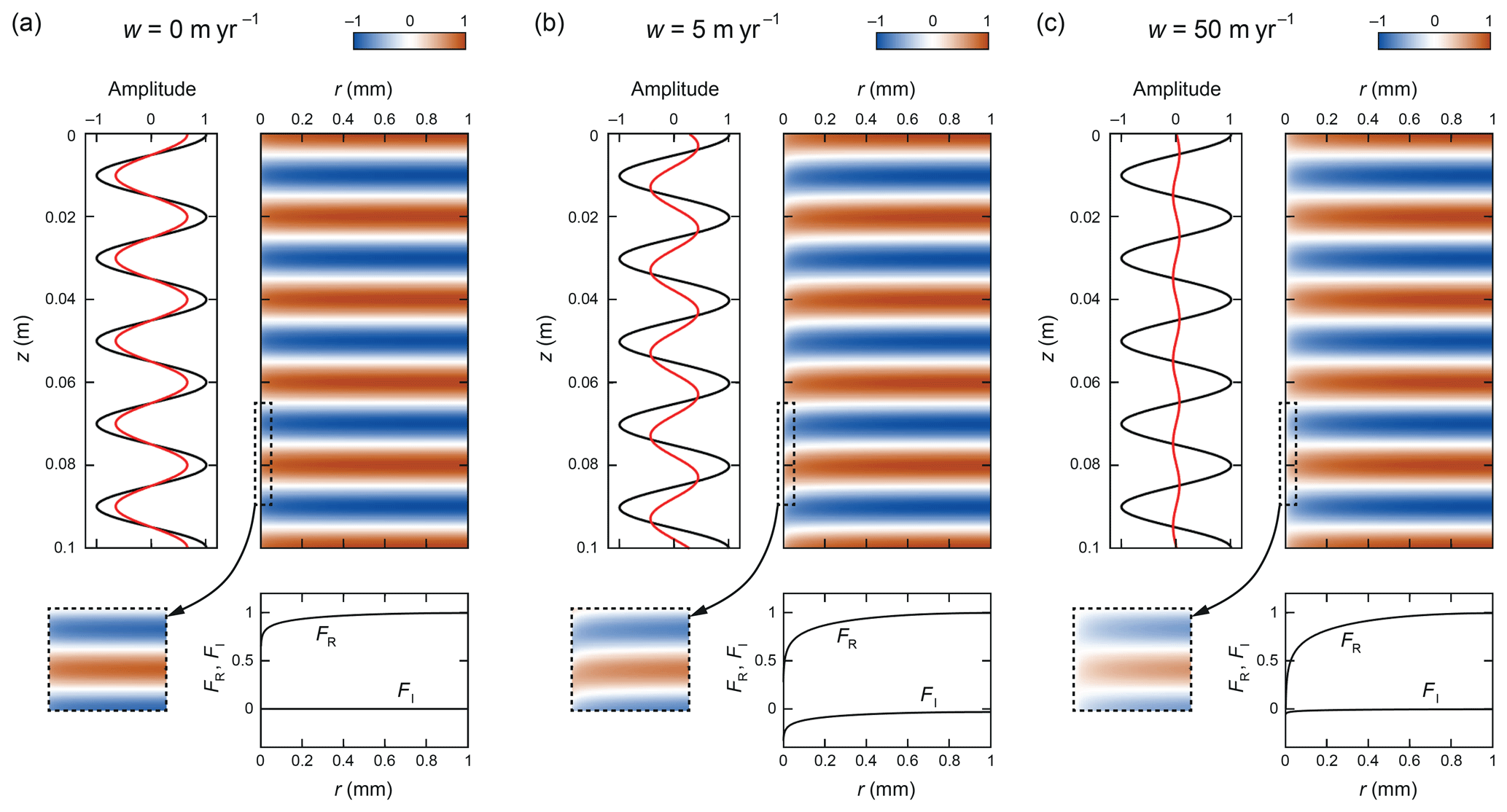
Figure 3 Patterns of δ calculated with Eqs. (7) to (15) for λ=0.02 m, $T=-\mathrm{32}$ ^∘C, and w equal to (a) 0, (b) 5, and (c) 50 m yr⁻¹. The enhancement factors in these experiments are f=2.11, 3.24, and 4.26, respectively. Each colour map samples a radial cross-section of the three-dimensional ice annulus in Fig. 1 and is shown with a horizontal exaggeration of 50. Dashed boxes expand on the details near r=0. The vein boundary lies at $r=a=\mathrm{1}$ µm. The panel under each map plots the real and imaginary parts of the amplitude function F(r). The panel left of each map plots the δ variations at the vein (red) and in the farthest part of the grain interior (r=b, black).

Figure 3 shows the computed pattern of δ in the ice annulus in three experiments with w=0, 5, and 50 m yr⁻¹ at λ=2 cm and $T=-\mathrm{32}$ ^∘C. All three signals decay with time; those in Fig. 3b and c migrate downward at constant velocity. We focus on examining the spatial part of the solution in Eq. (7) – the colour maps plot Re[F(r)exp(ik_zz)] (or $\left|F\right(r\left)\right|\cos (k_{z}z+\mathit{\theta }(r\left)\right)$, where θ is the signal phase defined earlier) without the time element. When plotting each pattern, we scale its amplitude such that $\left|F\right(b\left)\right|=\mathrm{1}$. This choice facilitates comparison of the δ variations along the vein with those at r=b.

Nye's short-circuiting occurs when w=0 (Fig. 3a), as expected. As we move from the grain interior towards the vein, the sinusoidal signals decrease in amplitude sharply following F(r), very close to the vein (dashed box, Fig. 3a). Consequently, isotopes diffuse from the grain interior towards the vein along the peak ridges of the signal, and in the opposite direction along troughs. This pattern of transverse isotopic exchange between vein and ice is driven by fast diffusion along the vein smoothing the signal there and is what causes the entire signal to decay faster than the baseline decay rate, $D_{\mathrm{s}}{k}_z^{\mathrm{2}}$ (as governed only by isotope diffusion vertically between the ridges and troughs). The enhancement factor in this experiment is f=2.11, as calculated by Rempel and Wettlaufer (2003).

When we switch on vein-water flow (Fig. 3b, c), f is amplified by a novel effect. Advection shifts the vein signal down relative to the interior, inducing a sheared pattern of δ variations in a thin layer next to the vein boundary, of negative phase (F_I<0). At w=5 m yr⁻¹ (Fig. 3b), the sinusoidal variations in the layer have a “tail-like” appearance in colour. Because their phase shift increases towards the vein, there are high lateral gradients in δ at the vein end of the signal peaks and troughs, and they drive a stronger diffusive isotopic exchange between vein and ice (than in the no-flow case), which accelerates the signal decay: f=3.24 in this case. The profile of F_R(r) and signal amplitude at r=a are correspondingly reduced.

When w is raised to 50 m yr⁻¹ (Fig. 3c), the shear layer becomes “sheet-like”. Strong advection causes δ outside the vein to interact with δ in the vein much higher up, and the coupling of this with diffusion in the ice diminishes the isotopic variations along and immediately outside the vein to near zero. One can think of the pattern in the layer now as due to the tails of high (low) δ extending far down to cover the next trough (ridge), with δ averaging out sideways by diffusion. Compared to the last experiment, the F_R profile is drawn down even more, the transverse isotopic exchange still stronger. The enhancement f=4.26 is nearly maximised, since the signal pattern is close to what it would be at the w→∞ limit, with no variations along the vein as in the Nye model (we confirmed this in experiments that took w above 50 m yr⁻¹).

The last finding implies that, at any signal wavelength, the high flow limit (w→∞) yields the same enhancement as the Nye model limit (β→∞). This equivalence arises because in Eq. (5) w→∞ drives $\partial \mathit{\delta }/\partial z{|}_{r=a}$ to zero, whereas β→∞ drives ${\partial }^{\mathrm{2}}\mathit{\delta }/\partial z^{\mathrm{2}}{|}_{r=a}$ to zero, and both yield the constant vein boundary condition δ≡δ₀ to precondition the same isotopic pattern. It follows that f at high flow in our model asymptotically reaches Nye's enhancement factor, and since f at w=0 is minimum (and equal to Rempel and Wettlaufer's enhancement factor), f must take an intermediate value in $\mathrm{0}<w<\mathrm{\infty }$.

Next we consider wavelength control. At fixed w, longer signals experience a higher decay-rate enhancement (though remember their baseline decay rate is lower). Figure 4 demonstrates this with a modified set of experiments, for λ=8 cm, at the same temperature and flow velocities as before. The shear-layer mechanism again operates when w>0. The tails lengthen as w is increased, although the pattern is still in the “tail regime” at 50 m yr⁻¹; at this longer wavelength, a higher w is needed to shift the variations far enough for transition to the “sheet regime”. In all three cases, f is higher (respectively ≈ 1.3, 3, and 12 times greater) than before. The reason lies in the relative contribution of (i) vertical diffusion between signal ridges and troughs and (ii) lateral diffusive exchange between vein and ice in driving the signal decay. For signals that are short compared to the grain radius (λ≪b), vertical diffusion dominates over lateral exchange, so vein-water flow increases f minimally via the shear-layer mechanism. For long signals (λ≫b), the lateral exchange is more significant, so the shear-layer mechanism amplifies f more strongly. Note that all three F_R profiles in Fig. 4 curve down less than those in Fig. 3, but the attendant reduced lateral exchange rates are still higher than the vertical diffusion rates, which are 16 times less at λ=8 cm than at λ=2 cm. Rempel and Wettlaufer (2003) made similar arguments to explain the wavelength control on f in the system without vein flow. Here we have added the shear-layer mechanism to the considerations.

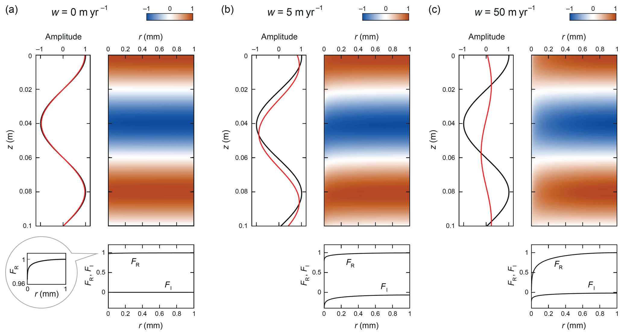
Figure 4 Patterns of δ computed for λ=0.08 m, $T=-\mathrm{32}$ ^∘C, and w equal to (a) 0, (b) 5, and (c) 50 m yr⁻¹. The enhancement factors in these experiments are f=2.63, 9.01, and 50.2, respectively. The figure has a similar layout as Fig. 3. The inset in panel (a) expands on the variations of F_R.

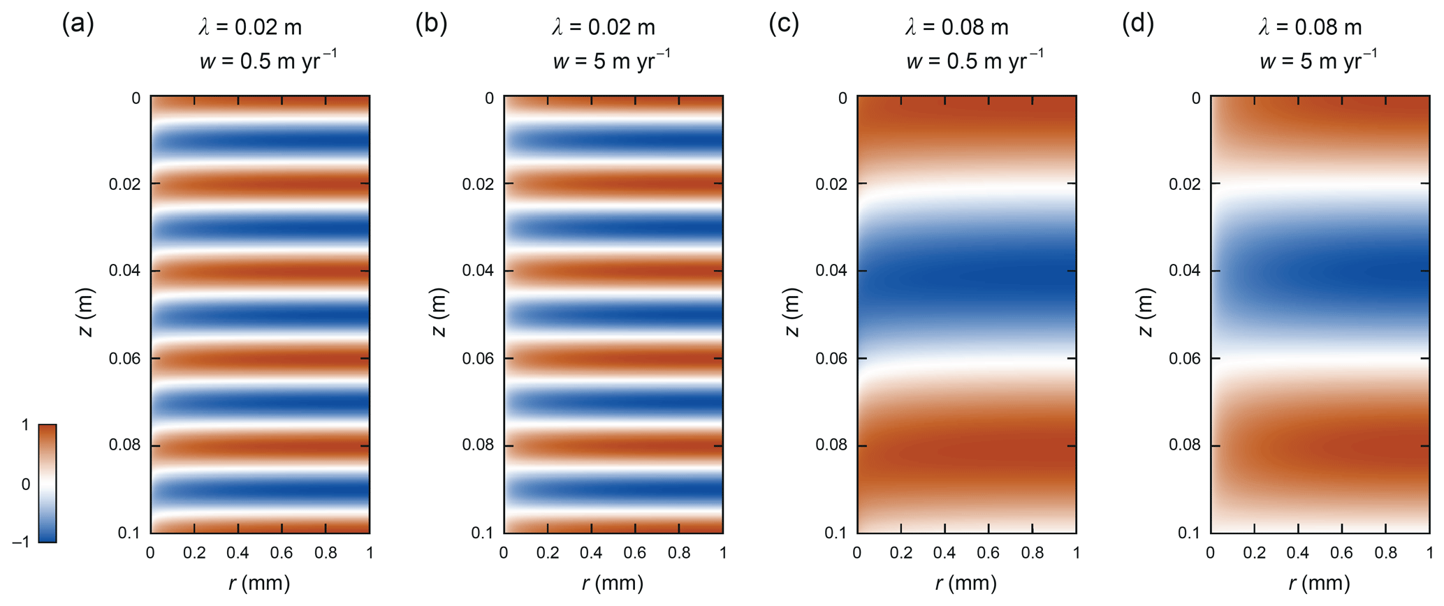
Figure 5 Patterns of δ computed for $T=-\mathrm{52}$ ^∘C at (a) λ=0.02 m, w=0.5 m yr⁻¹, (b) λ=0.02 m, w=5 m yr⁻¹, (c) λ=0.08 m, w=0.5 m yr⁻¹, and (d) λ=0.08 m, w=5 m yr⁻¹. The enhancement factors are f=3.68, 4.27, 14.7, and 51.9, respectively.

Results for colder ice ($T=-\mathrm{52}$ ^∘C, Fig. 5) predict higher enhancements at the same values of λ and w and shear-layer transitions at lower vein-flow velocities. For both the 2 and 8 cm signals, the tail-to-sheet transition is now largely complete when w reaches 5 m yr⁻¹ (Fig. 5; cf. Figs. 3 and 4). These changes are not due mainly to the change in diffusivity contrast $\mathit{\beta }(=D_{\mathrm{v}}/D_{\mathrm{s}}-\mathrm{1}$) but rather to the reduced D_s at low temperature (Fig. 2), which raises the importance of vein-flow-assisted lateral isotope exchange compared to vertical diffusion in the grains in smoothing the signal. We study the temperature control more below, where it will be seen that the dominance of these factors D_s and β reverses at low vein-flow velocities.

The mechanism detailed here – initiation of the shear layer by vein-water flow, its progression through the tail and sheet regimes as the magnitude of w is increased, and how the layer isotopic gradients amplify the short-circuiting to accelerate signal decay – is universal across our experiments. To help readers visualise the evolution, we show in Movies S1 and S2 continuous versions of Figs. 3 and 4, with w changing in small steps, covering upward as well as downward water flow.

Having explored the spatial interactions behind the decay-rate enhancement amplification, we report the influences of wavelength and vein-flow velocity more comprehensively by computing curves of f(λ) at fixed w (Fig. 6) and surfaces of f over the λ–w parameter space (Fig. 7). We do this for $T=-\mathrm{32}$ ^∘C and $T=-\mathrm{52}$ ^∘C, plotting log₁₀f and the signal migration velocity v also. Figures 6 and 7 confirm that f increases monotonically with λ and $\left|w\right|$, and, at each λ, f increases from Rempel and Wettlaufer's f value at w=0 towards a maximum (Nye's enhancement factor) as $\left|w\right|\to \mathrm{\infty }$. Importantly, while for centimetre- to decimetre-scale signals f is a few times without vein-water flow, it increases to ∼ 10¹–10² with vein-water flow. The increase is steepest at $\left|w\right|\sim \mathrm{10}$ to 20 m yr⁻¹ at −32 ^∘C and $\left|w\right|\sim \mathrm{1}$ m yr⁻¹ at −52 ^∘C. Accordingly, for the upper parts of ice cores from central Greenland, West Antarctica and coastal Antarctica, where $T\approx -\mathrm{20}$ to −30 ^∘C is common, the extra enhancement above Rempel and Wettlaufer's f is limited until w exceeds a few metres per year (Fig. 6a–b). For the upper parts of ice cores in central East Antarctica, such as at the EPICA Dome C, Dome Fuji, and Vostok ice-core sites, where $T\approx -\mathrm{50}$ ^∘C, the extra enhancement is already significant at w∼0.5 m yr⁻¹ (Fig. 6d–e). Results computed using the fractionation coefficients for oxygen and deuterium instead of α=1 (Figs. S1 and S2 in the Supplement) differ minimally from those in Figs. 6 and 7.

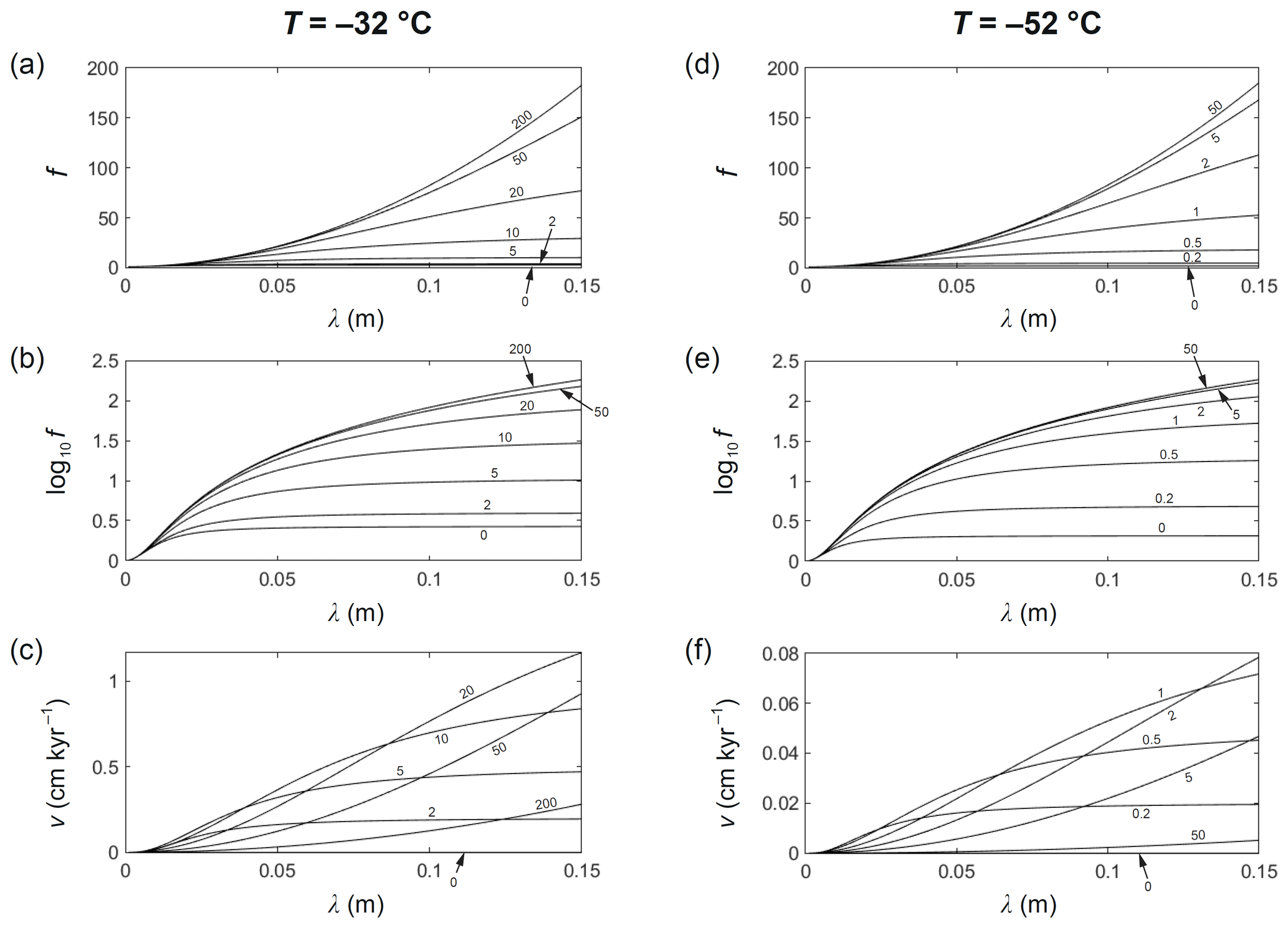
Figure 6 Computed curves of signal decay-rate enhancement factor f, log₁₀f, and signal migration velocity v versus signal wavelength λ, at (a–c) $T=-\mathrm{32}$ ^∘C and (d–f) $T=-\mathrm{52}$ ^∘C, for different vein-flow velocities w (labels by the curves, in m yr⁻¹). The lowest curves in f and log₁₀f portray Rempel and Wettlaufer's (2003) enhancement factor. The highest curves approach Nye's (1998) enhancement factor.

The surfaces of f at the two temperatures have similar shapes but different scales in w (Fig. 7). The surface for −52 ^∘C is in fact almost exactly a compressed version in the w direction of the surface for −32 ^∘C. Movie S3 illustrates this “compressional scaling”, as T varies from −20 to −60 ^∘C. The surface always approaches the same profile f(λ) as $\left|w\right|\to \mathrm{\infty }$ (also see Fig. 6a, d) to yield Nye's enhancement factor, which does not depend on temperature, because D_v and D_s do not enter the model to influence ζ when w→∞ or β →∞ (Eqs. 3 to 5) (remember the baseline decay rate does increase with T via D_s). However, the surface evolves not merely by compressional scaling. A subtle change also occurs in the valley near w≈0: there, f at −32 ^∘C exceeds f at −52 ^∘C slightly (the lowest curves in Fig. 6b and e). Consequently, as T is reduced, the surface contracts towards w=0, causing f to rise at moderate to large values of $\left|w\right|$ (yielding the earlier result that f decreases with temperature) but to drop near w≈0 (this is too small to be visible in Movie S3).

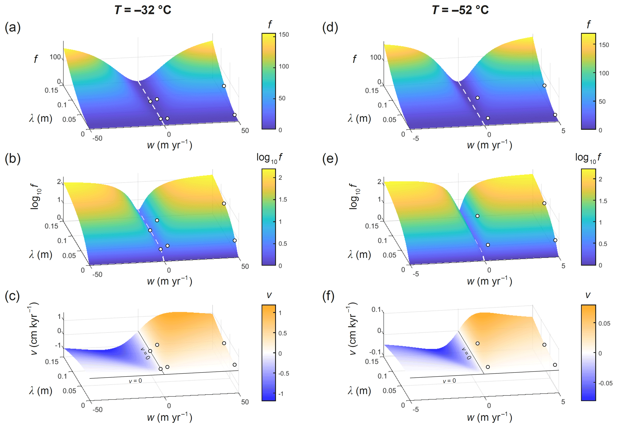
Figure 7 Computed signal decay-rate enhancement factor f, log₁₀f, and signal migration velocity v over the λ–w parameter space at (a–c) −32 ^∘C and (d–f) −52 ^∘C. Dashed white curves delineate f(λ) at w=0, which is the enhancement factor in Rempel and Wettlaufer's (2003) model. Circles locate the experiments of Figs. 3, 4, and 5. The curves in Fig. 6 are transects of these surfaces at fixed w.

These temperature controls can be explained by a model scaling analysis. As detailed in Appendix B, with constant vein and grain radii (a and b fixed), three dimensionless parameters govern the signal pattern in the ice annulus and the associated signal decay rate: (i) the ratio of the signal wavelength to the grain radius $\mathit{\lambda }/b$, (ii) the ratio of isotope advection by vein-water flow to isotope diffusion in the ice wb $/D_{\mathrm{s}}$, and (iii) the diffusivity contrast β (the Péclet number considered by Rempel and Wettlaufer, 2003, is a combination of these parameters). It follows that the enhancement factor f has the functional form $f(\mathit{\lambda }/b,wb/D_{\mathrm{s}},\mathit{\beta })$, whose shape is portrayed by the surfaces in Fig. 7. The influences of λ and w in the first two arguments of this function were explored in earlier experiments. A temperature change affects f via both its second and third arguments, because D_s and β vary with T (Fig. 2). The compressional scaling stems from the second argument, wb $/$ D_s. In contrast, the influence on f by the third argument β (over its range of interest, ∼ 10⁶) is weak and prevails only when f is small – near w≈0. There, f decreases when T is reduced from −32 to −52 ^∘C because a decrease in β (Fig. 2c) weakens the short-circuiting.

Turning to the migration velocity v (Figs. 6c, f; 7c, f), the model predicts signals to move in the direction of vein-water flow at speeds that reach a maximum at intermediate w and are higher for long signals and at high temperatures, of up to ∼ 1 cm kyr⁻¹. Most speeds on the parameter space are much lower. Hence, signal migration is slow, in the sense that long (at least millennial) timescales are needed to displace centimetre- and decimetre-scale annual signals against the ice and other ice-core proxies by a wavelength or more. The relative inaccuracy caused by this on the age scales determined through counting of δ cycles on isotope records is negligible. Compressional scaling applies also to v (Fig. 7, Movie S3), which has the form ($D_{\mathrm{s}}/b\left)g\right(\mathit{\lambda }/b,wb/D_{\mathrm{s}},\mathit{\beta }$) where the function g differs from f (Appendix B). The prefactor $D_{\mathrm{s}}/b$ explains why migration slows as temperature is reduced.

In their calculations, Rempel and Wettlaufer (2003) and Johnsen et al. (2000) accounted for the misorientation of veins from the vertical in the three-dimensional vein network by reducing D_v by a bulk tortuosity factor τ_f=3. Doing this in our experiments would lower β by ≈3 times and alter the results numerically but not change our qualitative findings.

4 Implications for diffusion-length studies

To explore how much excess diffusion modulated by vein-water flow impacts signal smoothing down the ice column, we simulate diffusion-length profiles for ice-core sites in Greenland and Antarctica, in a forward model testing w. We compare the results against profiles modelled without excess diffusion and query whether they match the level of excess diffusion inferred from isotope records. We also consider the impact on diffusion-length-based temperature reconstructions.

We use the well-established theory of Johnsen (1977) for these calculations, treating what happens below the firn only. In a moving coordinate system where z measures depth below a material horizon in the ice as it descends towards the bed, isotopic signals evolve according to

$$\begin{array}{}\text{(17)}& {\displaystyle \frac{\partial \overline{\mathit{\delta }}}{\partial t}}=D\left(t\right){\displaystyle \frac{{\partial }^{\mathrm{2}}\overline{\mathit{\delta }}}{\partial z^{\mathrm{2}}}}-{\dot{\mathit{\epsilon }}}_z\left(t\right)z{\displaystyle \frac{\partial \overline{\mathit{\delta }}}{\partial z}},\end{array}$$

where t is the age of the horizon, ${\dot{\mathit{\epsilon }}}_z$ (< 0) is the local vertical strain rate, and $\overline{\mathit{\delta }}$ is the section-mean signal in Eq. (16). Since the enhancement factor f applies to this signal (Sect. 2), the bulk-ice isotopic diffusivity in Eq. (17) is given by

$$\begin{array}{}\text{(18)}& D\left(t\right)=D_{\mathrm{s}}\left(T\right)f(\mathit{\lambda },w),\end{array}$$

where the dependence on age arises through T, λ, and other controls of f that vary as the signal descends (β, potentially also w, a, and b). We model a steady-state ice column with fixed temperature and ice velocity profiles. Given the ice thickness, the surface accumulation rate, and the strain-rate profile, the age–depth scale is determined, and signals with the wavelength λ₀ at the firn transition shorten to the wavelength $\mathit{\lambda }={\mathit{\lambda }}_{\mathrm{0}}S\left(t\right)/S(t_{\mathrm{0}}$) at age t, where $S\left(t\right)=\exp {\int }_{\mathrm{0}}^t{\dot{\mathit{\epsilon }}}_z\left(\mathit{\tau }\right)\mathrm{d}\mathit{\tau }\le$ 1 is the thinning function, and t₀ is the firn transition age. The normalisation of S by S(t₀), absent in studies that track signals from the ice-sheet surface, accounts for the minor thinning that has taken place by t=t₀.

According to Johnsen's (1977) solution of Eq. (17), one can track the amplitudes of different harmonics (Fourier components) of the signal separately³ by using the diffusion length σ, which measures the root mean square distance travelled by diffusing isotopes. Specifically, the squared diffusion length σ² obeys the differential equation

$$\begin{array}{}\text{(19)}& {\displaystyle \frac{\mathrm{d}{\mathit{\sigma }}^{\mathrm{2}}}{\text{d}t}}-\mathrm{2}{\dot{\mathit{\epsilon }}}_z\left(t\right){\mathit{\sigma }}^{\mathrm{2}}=\mathrm{2}D\left(t\right),\end{array}$$

and each harmonic attenuates by the ratio $R=\exp (-\mathrm{2}{\mathit{\pi }}^{\mathrm{2}}{\mathit{\sigma }}^{\mathrm{2}}/{\mathit{\lambda }}^{\mathrm{2}})$ as σ and λ evolve down column. It follows that a harmonic is attenuated strongly when its wavelength shortens to less than σ (e.g. Gkinis et al., 2021). In our simulations, we specify an initial value σ=σ_firn at the firn transition – taken from studies of firn isotope diffusion – to circumvent the need to model firn processes. The ratio tracking signal amplitude in the ice is then

$$\begin{array}{}\text{(20)}& R_{\mathrm{i}}=\exp \left[-\mathrm{2}{\mathit{\pi }}^{\mathrm{2}}({\mathit{\sigma }}^{\mathrm{2}}/{\mathit{\lambda }}^{\mathrm{2}}-{\mathit{\sigma }}_{\text{firn}}^{\mathrm{2}}/{\mathit{\lambda }}_{\mathrm{0}}^{\mathrm{2}})\right].\end{array}$$

Following Gkinis et al. (2014), we decompose σ² into a part due to isotopic diffusion in ice, ${\mathit{\sigma }}_{\mathrm{ice}}^{\mathrm{2}}$, and another part inherited from firn isotopic diffusion that thins under the compression; thus,

$$\begin{array}{}\text{(21)}& {\mathit{\sigma }}^{\mathrm{2}}\left(t\right)={\mathit{\sigma }}_{\text{ice}}^{\mathrm{2}}\left(t\right)+{\mathit{\sigma }}_{\text{firn}}^{\mathrm{2}}{\left[{\displaystyle \frac{S\left(t\right)}{S\left(t_{\mathrm{0}}\right)}}\right]}^{\mathrm{2}}.\end{array}$$

Substituting for σ² in Eq. (19), using Eq. (18) for D, yields

$$\begin{array}{}\text{(22)}& {\displaystyle \frac{\mathrm{d}{\mathit{\sigma }}_{\text{ice}}^{\mathrm{2}}}{\text{d}t}}-\mathrm{2}{\dot{\mathit{\epsilon }}}_z{\mathit{\sigma }}_{\text{ice}}^{\mathrm{2}}=\mathrm{2}{D}_{\mathrm{s}}f(\mathit{\lambda },w),\end{array}$$

with σ_ice=0 at t=t₀. This equation is straightforward to solve analytically by an integrating factor (Gkinis et al., 2014) or numerically by the finite-difference method (as done in our simulations below).

In reconstructions of firn temperature (e.g. Gkinis et al., 2014; Holme et al., 2018), Eq. (21) is rearranged as

$$\begin{array}{}\text{(23)}& {\mathit{\sigma }}_{\text{firn}}^{\mathrm{2}}={\displaystyle \frac{{\mathit{\sigma }}_{\text{obs}}^{\mathrm{2}}-{\mathit{\sigma }}_{\text{ice}}^{\mathrm{2}}}{[S/S(t_{\mathrm{0}}){]}^{\mathrm{2}}}},\end{array}$$

to allow σ_firn at a given age to be found from (i) the thinning S, (ii) the modelled value of σ_ice (from Eq. 22), and (iii) the diffusion length σ_obs estimated from isotopic signals in the ice core – at the same age. Firn isotope diffusion modelling is then used to invert σ_firn for temperature. The estimation of σ_obs involves fitting $P_{\mathrm{0}}\left(k\right)=P_{\mathrm{0}}{R}^{\mathrm{2}}=P_{\mathrm{0}}\exp (-k^{\mathrm{2}}{\mathit{\sigma }}^{\mathrm{2}})$ ($k=\mathrm{1}/\mathit{\lambda }$ is the wavenumber) to the power spectral density (PSD) graph of the measured signals, assuming a white-noise input signal at the surface, i.e. constant P₀; see Kahle et al. (2018) for different approaches to this estimation.

Equation (22) reveals a notable consequence of excess diffusion (f>1) for the diffusion-length estimation. Besides raising σ_ice (thus σ) to accelerate signal decay, excess diffusion makes σ_ice wavelength dependent: this does not arise if the bulk ice has Ramseier's diffusivity (f≡1), as assumed in most past studies. With excess diffusion, σ_ice varies with λ and the initial wavelength λ₀, so the harmonic components have different diffusion-length histories. Their spectral power now decays as exp(−k²σ²), where σ decreases with k (rather than being constant), as f increases with λ (Sect. 3). Since f=1 at zero λ only (Figs. 6 and 7), σ exceeds the σ value for monocrystalline ice at all k<∞. Fitting of the resulting non-parabolic PSD thus overestimates σ_obs, in the context of firn-temperature reconstructions assuming Ramseier's diffusivity for the ice in Eqs. (22) and (23).

More precisely, our model implies that fitting exp(−k²σ²) to the PSD decay of the signal to find σ is no longer appropriate when excess diffusion operates; strictly speaking, the fit should be made with exp$[-k^{\mathrm{2}}({\mathit{\sigma }}_{\mathrm{ice}}^{\mathrm{2}}+({\mathit{\sigma }}_{\mathrm{firn}}S/S(t_{\mathrm{0}}\left){)}^{\mathrm{2}}\right)]$ to find σ_firn, with σ_ice (solution of Eq. 22) varying with k and w. We demonstrate the wavelength dependence of σ_ice in simulations below. The dependence does not arise in the firn, because σ_firn is not a function of λ, according to models of firn isotope diffusion (Whillans and Grootes, 1985; Johnsen et al., 2000; Gkinis et al., 2014, 2021). Note that when the diffusion length σ develops wavelength dependence, it refers to the root mean square displacement of isotopes only if the signal (at a given depth) has a single wavelength, not if it is composed of multiple harmonics.

We proceed to examine diffusion-length profiles computed for ice-column conditions based on the GRIP site in Greenland and the EPICA Dome C site in Antarctica (Fig. 8). For these sites we specify σ_firn=8 and 7 cm, respectively (e.g. Fig. S2 of Gkinis et al., 2014). Most of our model runs assume a=1 µm and b=2 mm, although some prescribe a variable grain-radius profile from measurements (Fig. 8d, h). We set α≡1 again, and we set 65 m as the firn transition depth. The age–depth scales yield t₀=286.3 a for GRIP and 2872.9 a for EPICA. At the firn transition, the wavelength of annual signals is given approximately by the ice-equivalent surface accumulation rate: 0.23 m yr⁻¹ at GRIP and 0.023 m yr⁻¹ at EPICA.

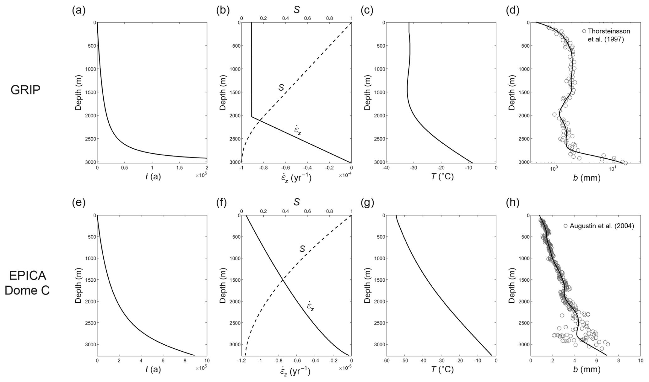
Figure 8 Depth profiles of glaciological variables used in our diffusion-length modelling for the (a–d) GRIP and (e–h) EPICA Dome C ice-core sites. (a, e) Age–depth scale. (b, f) Strain rate ${\dot{\mathit{\epsilon }}}_z$ and the associated thinning function S. (c, g) Ice temperature. (d, h) Grain-radius data (circles) and spline curves used in our modelling. Ice flow at the GRIP site assumes the Dansgaard–Johnsen model with ice thickness H=3029 m, kink height at 1000 m, and surface accumulation rate a_s=0.23 m yr⁻¹ ice equivalent. Ice flow at the EPICA site assumes the ice submergence velocity $w_{\mathrm{i}}=m_{\mathrm{b}}+(a_{\mathrm{s}}-m_{\mathrm{b}})(h/H{)}^{\mathrm{1.7}}$, where H=3275 m, a_s=0.023 m yr⁻¹ ice equivalent, h is height above the bed, and m_b=0.0008 m yr⁻¹ is the basal melt rate. See Ng (2021) for additional details about these profiles.

Figure 9a–d presents σ profiles simulated at GRIP for the annual signal (λ₀=0.23 m) alongside profiles of the enhancement f, ice diffusion length σ_ice, and the ratio R_i tracking signal amplitude. At each depth, σ increases with w via its modulation on σ_ice. Whereas excess diffusion with w=0 (no vein-water flow) raises σ and σ_ice slightly above their values based on Ramseier's diffusivity (f=1), w from several to tens of metres per year increases and modulates σ_ice significantly, with a strong impact on signal decay, down to ≈2300 m depth. From about half way down the column, the amount of excess diffusion diminishes rapidly with depth (f→1) due to severe shortening of the signal and increasing temperature (Sect. 3). The σ and σ_ice profiles converge on the profiles for f=1 near the base of the column because of this, because the firn part of σ is vanishing, and because the long time spent by deep ice at similar strain rate and temperature allows the effects of isotopic diffusion and vertical compression to balance, with σ_ice equilibrating to ($-D_{\mathrm{s}}\left(T\right)/{\dot{\mathit{\epsilon }}}_z{)}^{\mathrm{1}/\mathrm{2}}$ in Eq. (22).

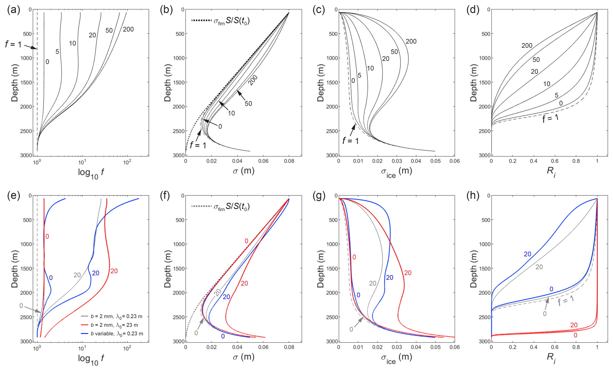
Figure 9 Computed depth profiles for the GRIP core site of (a, e) the enhancement factor f (representing excess diffusion above the monocrystal diffusivity), (b, f) diffusion length σ, (c, g) ice diffusion length σ_ice, and (d, h) signal amplitude ratio R_i. The number by each curve indicates the vein-water flow velocity w in metres per year (m yr⁻¹). In panels (a) to (d), all model runs study the annual signal (λ₀=0.23 m), assuming the grain radius b=2 mm; the dashed curves show results based on Ramseier's (1967) monocrystal diffusivity, i.e. f=1; and the dotted curve in panel (b) shows the thinned firn diffusion length. In panels (e) to (h), blue curves report results based on the variable grain-radius profile in Fig. 8d; red curves report results computed for signals with λ₀ a hundred times longer; and grey curves show selected results from panels (a) to (d) for comparison.

The model run for w=20 m yr⁻¹ in Fig. 9a–d mimics the diffusivity enhancement f∼10–30 found for annual signals in the GRIP Holocene ice by Johnsen et al. (1997, 2000), predicting also the reduced excess diffusion in deeper ice (> 1600 m) dating to the Younger Dryas and the last glacial alluded to in those studies. Although blockage of veins by the high dust content in stadial and glacial ice might explain this reduction (Johnsen et al., 1997, 2000), our model predicts a strong dependence of f on the shortening signal wavelength when w>0 (Fig. 6a, b) that provides an explanation. These considerations are unchanged if the run uses variable grain radius (Fig. 9e–h, blue curves for 20 m yr⁻¹). In contrast, the large enhancement f∼10–30 cannot be reproduced with w=0 (Rempel and Wettlaufer's (2003) model) with constant or variable b (Fig. 9e–h), not unless very large vein radii of ∼ 20 to 200 µm are assumed.

The wavelength dependence of σ and σ_ice is apparent from two runs that study a signal with an initial wavelength 100 times longer than the annual signal (red curves in Fig. 9e–h; cf. grey curves). The dependence strengthens with w; we analyse its depth variations later. Even with strong excess diffusion (when w=20 m yr⁻¹), the long signal survives much deeper than the annual signal (to ≈2800 m; Fig. 9h) because its baseline decay rate is 10⁴ times lower.

Turning to the EPICA site, our interest is drawn to long signals because annual signals are too short to survive isotopic diffusion in the firn (e.g. for λ=0.023 m, the firn attenuation is $R=\exp (-\mathrm{2}{\mathit{\pi }}^{\mathrm{2}}{\mathit{\sigma }}_{\mathrm{firn}}^{\mathrm{2}}/{\mathit{\lambda }}^{\mathrm{2}})\sim {\mathrm{10}}^{-\mathrm{80}}$). Figure 10a–c presents model runs for a millennial-scale signal with λ₀=23 m. They show a similar modulation of the f and σ profiles by w as seen in the GRIP runs; however, colder ice in the top half of the EPICA column than at GRIP (Fig. 8g, c) means that these profiles are more sensitive to w (Sect. 3). The modulation at EPICA extends to nearer the base of the ice column because the lower strain rate (which shortens signals more slowly and slows the equilibration in Eq. 22) causes σ to approach the f=1 curve slowly. The millennial signal survives into the deepest ice if w≲30 m yr⁻¹ (Fig. 10c).

What conditions at EPICA can produce the long diffusion lengths σ ∼ 40 to 60 cm inferred for ice at the depth of MIS 19 (∼ 3170 m) and thus strong suppression of millennial signals and near-complete absence of sub-millennial signals there? Pol et al. (2010) surmised excess diffusion as necessary. Like the σ profile they simulated, our result for f=1 yields only σ≈16 cm at that depth (Fig. 10b). The runs with excess diffusion at constant b show that w≈80 to 150 m yr⁻¹ generates enough excess diffusion, but the corresponding σ profiles bulge at ≈1000 m to attenuate the millennial signal strongly mid-column (Fig. 10b, c). Other ways of achieving σ∼ 40 to 60 cm in the deepest ice, with small or no bulge in σ that allows a sizeable signal to survive past ≈ 2500 m depth but not to ≈ 3100 m, are shown in Fig. 10d–g. They assume w profiles ramping up towards the bed – linearly, parabolically, or linearly/nonlinearly near the base – that all require w≳150 m yr⁻¹ in deep ice. If we further consider that Pol et al. (2011) estimated the diffusion length σ∼ 8 cm for ice at MIS 11 (∼ 395 to 426.7 ka, ∼ 2699 to 2799 m) in the EPICA core, then the run using the deep nonlinear w profile (red) best mimics the observations. In any case, excess diffusion unassisted by high vein-water flow at depth cannot explain them. The limited excess diffusion at w= 0, which hardly alters the signal evolution predicted by Ramseier's diffusivity (Fig. 10), is far from sufficient.

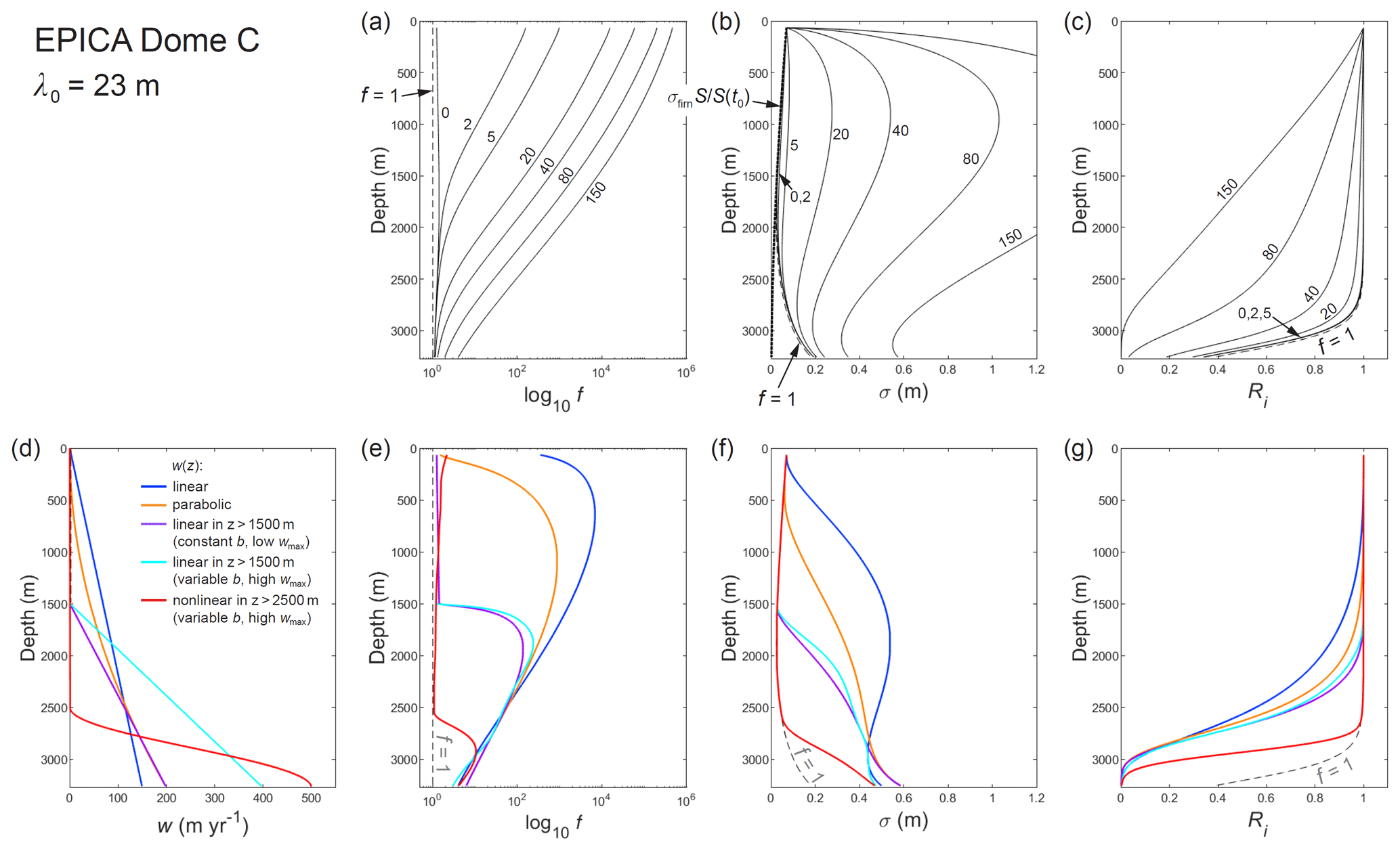
Figure 10 Computed depth profiles for the EPICA Dome C core site of (a, e) enhancement factor f, (b, f) diffusion length σ, and (c, g) signal amplitude ratio R_i. All model runs investigate a millennial-scale signal with λ₀=23 m (1000 × annual layer thickness based on surface accumulation rate). In panels (a) to (c), each run assumes b=2 mm and constant vein-water flow velocity w (value beside each curve, m yr⁻¹). Curves labelled f=1 show results based on Ramseier's diffusivity. Panels (e) to (g) report five model runs able to yield σ of 0.4–0.6 m near the base, assuming the variable w profiles in panel (d). Three runs assume b=2 mm, and two runs assume the variable grain-radius profile in Fig. 8h.

In summary, for both the GRIP and EPICA cores, vein-flow modulation with suitable choices of w can reproduce the levels of excess diffusion inferred from their isotope records. Nye's model (which is approached at high w in Figs. 9 and 10, as w→∞ regains his model; Sect. 3) and Rempel and Wettlaufer's model (w=0) overpredict and underpredict those levels, respectively, in simulations using grain sizes similar to those measured. The reason Rempel and Wettlaufer's model revises down Nye's enhancement factor f was explained in Sects. 2 and 3. Accounting for vein tortuosity (by lowering D_v) weakens the short-circuiting and reduces f further and does not alter these findings.

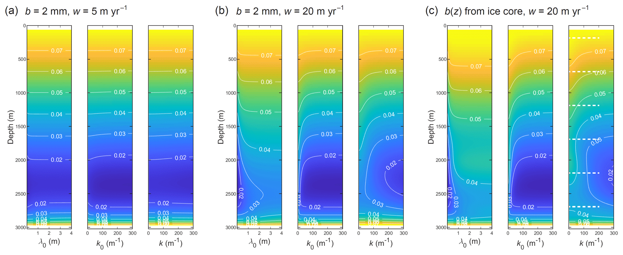
Figure 11 Wavelength dependence of the diffusion length σ (colour, contours in m) at the GRIP site for three parameter settings: (a) w=5 m yr⁻¹, b=2 mm; (b) w=20 m yr⁻¹, b=2 mm; and (c) w=20 m yr⁻¹ with the grain-radius profile in Fig. 8d. In each panel, the maps plot σ versus depth against the initial wavelength of the signal λ₀, its initial wavenumber k₀, and its wavenumber k at depth. The dashed white lines on the map at far right locate the transects of Fig. 12a.

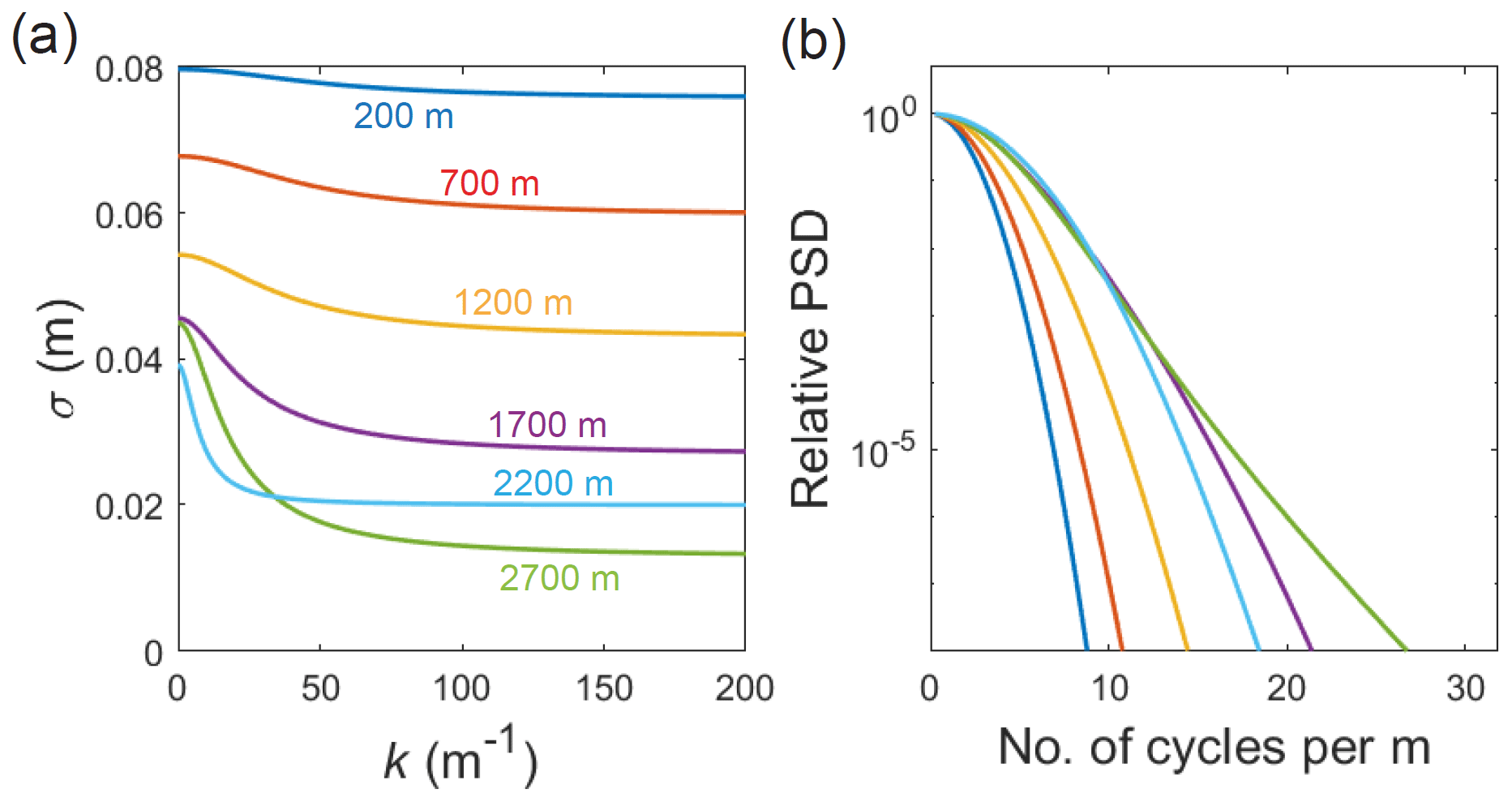
Figure 12 (a) Diffusion length σ as a function of signal wavenumber k, computed at six depths in the GRIP ice column (numbers in colour) in the model runs in Fig. 11c, assuming w= 20 m yr⁻¹ and the variable grain-radius profile. (b) Synthetic power spectral density (PSD) decays based on the curves in panel (a), colour coded as there. Each signal with wavenumber k has $k/\mathrm{2}\mathit{\pi }$ cycles per metre, so the horizontal axes in panels (a) and (b) are equivalent.

And what of the implications for firn temperature reconstructions? Excess diffusion can bias them in two ways, which we discuss here using the GRIP runs as an example.

First, it introduces uncertainty and bias to σ_obs found by PSD fitting. Figure 11 maps the computed diffusion length versus depth for signals of different initial wavelength λ₀ (think of the left-most plot of each panel as showing multiple σ profiles in a stack); in the same way, it maps σ against their initial wavenumber $k_{\mathrm{0}}=\mathrm{1}/{\mathit{\lambda }}_{\mathrm{0}}$ and their wavenumber at depth after accounting for thinning, $k=k_{\mathrm{0}}S\left(t_{\mathrm{0}}\right)/S$. Whether the simulations use a constant or variable grain radius, σ develops a pronounced wavelength dependence at w=20 m yr⁻¹ (the velocity yielding the level of excess diffusion in GRIP Holocene ice) at most depths, except near the surface and base (Fig. 11b, c). As anticipated, σincreases with λ₀ and decreases with k monotonically. Its variations (> 15 % below 700 m; Fig. 12a) mean that the PSD decays [∝ exp(−k²σ²(k))] are not parabolic in k as they might seem (Fig. 12b). Consequently, σ_obs found by fitting exp($-k^{\mathrm{2}}{\mathit{\sigma }}_{\mathrm{obs}}^{\mathrm{2}}$) to the decays will be misestimated and, as explained earlier, biased too high for existing firn-temperature reconstructions (by an amount dependent on the fitting method).

This issue will arise wherever excess diffusion occurs and in deeper ice below any section with excess diffusion. It will affect reconstructions using the difference between the diffusion lengths of oxygen and deuterium (Simonsen et al., 2011; Holme et al., 2018) as well as those reconstructions using the diffusion length of a single isotope. It can be diagnosed by a statistically significant negative trend in log(PSD)$/k^{\mathrm{2}}$ over k, although real PSD data contain noise and artefacts related to the ice-core isotopic measurements (e.g. Kahle et al., 2018) that may complicate such a test.

Second, excess diffusion affects the calculation of σ_firn in Eq. (23) – via the magnitude of σ_ice. Temperature reconstructions based on diffusion length (Gkinis et al., 2014; Holme et al., 2018; Gkinis et al., 2021; Kahle et al., 2021) typically use Ramseier's diffusivity to find σ_ice (i.e. Eq. 22 with f=1), which is justified for ice cores where excess diffusion does not operate. But where it does operate, σ_ice is underestimated, and σ_firn and the reconstructed firn temperature are overestimated: accounting for excess diffusion would yield a lower temperature. Put another way, a high σ_obs at a given depth may result from a large (thinned) σ_firn contribution from high firn temperature in the past, from excess diffusion that raised σ_ice, or from both. Robust inversion for σ_firn must therefore ascertain the amount of excess diffusion.

The impact on σ_firn in single-isotope reconstructions can be gauged using the GRIP runs. Figure 9c and g show that the underestimation of σ_ice by Ramseier's diffusivity is minimal at w=0, but it reaches ∼ 0.01 to 0.02 m (to ≈ 2000 m depth) if w=20 m yr⁻¹. To gauge how much σ_firn is perturbed, we calculate σ_firn in Eq. (23) by using σ profiles simulated in forward runs at different w as the input for σ_obs, but using the profile of σ_ice at f=1 as the other input. These tests thus imitate Ramseier-based reconstructions applied to isotope records influenced by excess diffusion, although they are not comprehensive, as our runs used a fixed imposed history of σ_firn≡0.08 m rather than time-varying σ_firn. The results show that σ_firn is overestimated by an amount increasing with depth and w (Fig. 13). When w=20 m yr⁻¹, σ_firn is too high by ∼0.02 m between 1000 and 2000 m depths (ca. 5.5–17 ka), and the overestimation increases from ∼0.01 to 0.03 m through this depth range. With the typical sensitivity of the firn-temperature inversion for Greenland (Fig. S2 of Gkinis et al., 2014; Fig. 3 of Gkinis et al., 2021), a deviation in σ_firn of ±0.02 m around 0.08 m translates to a temperature change of ≈ ± 5 ^∘C. Hence, the firn temperature in this scenario will be overestimated by Ramseier-based reconstructions by several degrees, increasing (with age) through the Holocene and the period since the Last Glacial Maximum.

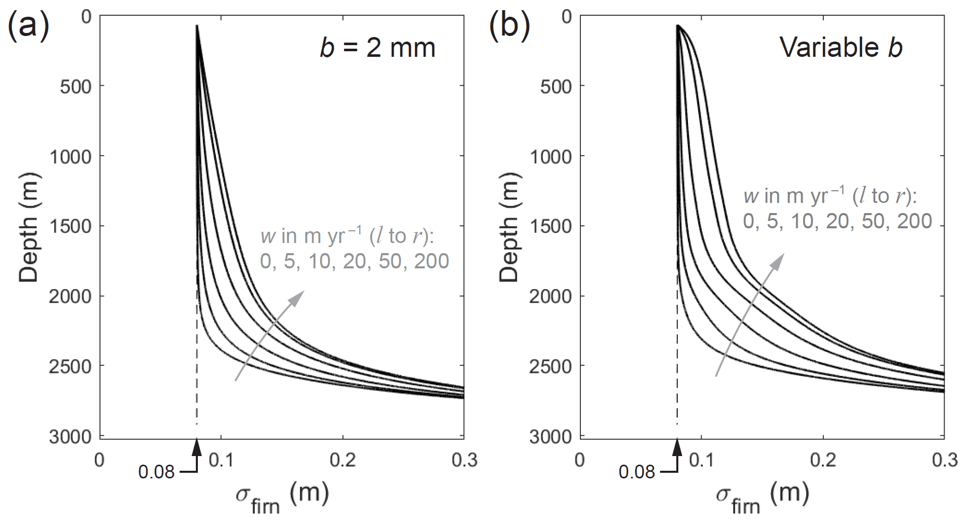
Figure 13 Firn diffusion length σ_firn recovered using Eq. (23), with σ_obs taken from the diffusion-length profiles simulated in forward runs at the GRIP site (for scenarios with excess diffusion at different water-flow velocities w), and with σ_ice calculated by assuming Ramseier's diffusivity for the bulk ice. The forward runs are based on b=2 mm in panel (a) and based on the measured (variable) grain-size profile in panel (b).

In this connection, Gkinis et al. (2014) reconstructed a temperature history from δ¹⁸O in the NGRIP (North Greenland Ice Core Project) ice core (retrieved 325 km NNW of GRIP), which they regarded as ≈ 3 to 5 ^∘C too warm from ∼ 8 to 12 ka when compared to other reconstructions (see their Fig. 6). They down-adjusted their temperature results by modifying the thinning function S to reflect lower past accumulation rates. Although the glaciological conditions at NGRIP and GRIP differ, our results show that adjustments of this size are possible with vein-flow modulated excess diffusion. This is not to say that excess diffusion with w∼20 m yr⁻¹ occurred at NGRIP – we are not aware of reports of excess diffusion for that core. However, we recommend that diffusion-based temperature reconstructions assess whether their results could be biased by excess diffusion, besides considering the choices and uncertainties related to firn modelling (Gkinis et al., 2021) and diffusion-length estimation (Kahle et al., 2018). Our test case with w=20 m yr⁻¹ at GRIP is exemplative. Any bias will depend on the magnitude, distribution, and temporal variations of w.

Dual-isotope reconstructions should be less affected by this problem. These reconstructions exploit the different diffusion lengths of δ¹⁸O (or δ¹⁷O) and δD in the firn, as caused by the different fractionation coefficients (α) for ¹⁸O–¹⁶O (or ¹⁷O–¹⁶O) and D–H; specifically, they use the square differential Δσ²=σ²(oxygen) − σ²(deuterium) as the proxy for firn temperature (Simonsen et al., 2011; Holme et al., 2018). If the profiles of σ_ice were identical for oxygen and deuterium, as implied by our model of excess diffusion with α≡1 (and by Ramseier-based models), then neither the size of σ_ice nor the bias on σ_ice matter, because ${\mathit{\sigma }}_{\mathrm{ice}}^{\mathrm{2}}$ cancels out in the differencing. But the cancellation is imperfect because oxygen and deuterium differ slightly in their fractionation coefficients. To study the effect, we repeated the GRIP runs by using their α values in Eq. (15) to compute the corresponding σ_ice profiles and the ice part of the differential, $\mathrm{\Delta }{\mathit{\sigma }}_{\mathrm{ice}}^{\mathrm{2}}={\mathit{\sigma }}_{\mathrm{ice}}^{\mathrm{2}}$(oxygen) − ${\mathit{\sigma }}_{\mathrm{ice}}^{\mathrm{2}}$(deuterium). When w∼10 to 50 m yr⁻¹, $\mathrm{\Delta }{\mathit{\sigma }}_{\mathrm{ice}}^{\mathrm{2}}$ reaches ∼ 10⁻⁵ m² mid-column (Fig. S3). Since the observed variations in Δσ² for central Greenland fall in the range ∼ 10⁻⁴–10⁻³ m² (e.g. Figs. 2 and 3 of Simonsen et al., 2011), the ice contribution to the differential can bias dual-isotope reconstructions slightly where excess diffusion operates.

We have not repeated the foregoing analyses for the EPICA ice column because information about its pattern of excess diffusion, which is limited to the σ estimates for MIS 19 and MIS 11 (Pol et al., 2010, 2011), is less complete than at GRIP.

5 Conclusions and outlook

In this paper, we described a mechanism whereby vein-water flow amplifies the short-circuiting conceived by Nye (1998), enhancing the rate of isotopic diffusion in polycrystalline ice above the rate predicted by Rempel and Wettlaufer's (2003) model. Our simulations demonstrate its profound impact on signal smoothing in ice where the vein-water flow velocity w reaches ∼ 10¹–10² m yr⁻¹. We explained why vein-flow modulated excess diffusion biases the spectral estimation of diffusion lengths from isotope records, as well as diffusion-based palaeothermometry at ice-core sites. Our findings contribute insights essential for developing robust interpretation of ice-core isotope records.

Potential modulation of excess diffusion by vein-water flow means that ice-core isotopic signals may have been altered in more complex ways than previously thought. Where modulation occurs, neither Ramseier's (1967) formula nor Rempel and Wettlaufer's (2003) model describe the bulk-ice isotopic diffusivity, and we caution their use in ice-core analysis.

Our GRIP and EPICA simulations (Sect. 4) represent a detailed exploration of the impact of excess diffusion on diffusion-length profiles and probe the conditions behind the levels of excess diffusion inferred for those cores. Their expository nature should be emphasised: we have not fitted the observations precisely, and the vein-flow velocities in our model runs are only trial values in a sensitivity analysis. Several reasons preclude bespoke modelling for accurate validation or prediction at present. First, the model idealises the system geometry. Based on Nye's and Rempel and Wettlaufer's set-up (Fig. 1), it conceptualises the vein network in three dimensions by using a uniform array of cells and approximates the vein cross-section – which in reality consists of three convex faces (Nye, 1989; Mader, 1992a) – as circular. It also assumes that veins are static features, even though grain-boundary migration implies a continual slow motion of veins relative to crystal matrices (Ng, 2021), which will perturb the isotope concentration fields within ice grains. Second, the model ignores isotope diffusion along grain boundaries (Johnsen et al., 2000), which may further enhance excess diffusion in fine-grained ice (Jones et al., 2017). Third, some material properties serving as model inputs are subject to uncertainty. In particular, the formulae we use for the diffusivities D_s and D_v may only be reliable to within a factor of several; they neglect the potential influence of pressure and dissolved ionic impurities (which may change the fractionation coefficients also). The uncertainty involved is probably not dissimilar in magnitude to that associated with the geometrical approximation, and our qualitative findings (predicated on $D_{\mathrm{v}}/D_{\mathrm{s}}\gg \mathrm{1}$) are robust against it; how numerical results vary in our model if D_s and D_v are altered is also straightforward to compute. However, this uncertainty impacts all key modelling studies of excess diffusion to date (Nye, 1998; Johnsen et al., 2000; Rempel and Wettlaufer, 2003; the present study), so there is a clear need for more comprehensive laboratory determination of both diffusivities. Fourth, in simulations made for specific ice-core sites, two factors besides w are challenging to constrain: (i) suppression of the short-circuiting due to blockage of veins by dust particles and bubbles and (ii) spatial variation in vein radius. The vein size in ice at thermodynamic equilibrium should depend locally on the mean grain size, temperature, and amount of dissolved ionic impurities in the veins (Nye, 1991; Mader, 1992b; Dani et al., 2012). Consequently, factors (i) and (ii) suggest possible influences by changing vein-impurity signals (Ng, 2021) and changing distributions of bubbles and solid particles on excess diffusion and the smoothing of isotopic signals. Extending the model for these controls and the detailed geometry of the vein network as grain size and texture evolve are worthwhile avenues for further research.

A striking realisation from our study is how little is known about the vein-scale hydrology of ice sheets. The vein-flow velocity w is needed for predicting excess diffusion with the model or validating model runs made to match diffusion lengths measured from ice cores. However, reliable prediction of the size and pattern of w at ice-core sites is out of reach. Our only handle on w is Nye and Frank's (1973) theory for glaciostatically driven porewater flow. This theory calculates the rate of (Poiseuille) flow through veins under the hydropotential gradient (ρ_w−ρ_i)g, where ρ_w is water density, ρ_i is ice density, and g is gravitational acceleration. It yields a large range of plausible w because the ice porosity – a key input that determines the vein size for a given mean grain size – is uncertain for polar ice. When modelling the profile of w above subglacial lakes, Rempel (2005) combined Nye and Frank's (1973) theory with an equation of vein-equilibrium thermodynamics to constrain the porosity through the influence of dissolved impurities. Although this approach can predict specific values of w, it requires knowledge (or assumption) about the amount of ionic impurities partitioned to the vein network, which is not resolved by most ice-core analytical measurements. Besides, neither Rempel's nor Nye and Frank's model has been observationally tested. A separate theory by Nye (1976) treats vein-water flow in detail but analyses only its stability, not flow rates. Thus, currently, knowledge about w in polar ice is limited to a few embryonic theories, and we cannot evaluate whether the range of w values found to modulate excess diffusion sensitively are common at ice-core sites.

Direct measurements of vein-water flow in polar ice are critical for progress, for informing studies of excess diffusion and hydrological modelling. Vein size measurements at low temperature are also desirable, because the observations of Mader (1992b) (vein widths ∼10–100 µm) were made only within 1 ^∘C below the melting point. It may be possible to measure w by innovating on nuclear magnetic resonance (NMR) and Doppler-based techniques. Laboratory studies should couple vein size and flow measurements with experiments where water percolates through ice containing isotopic signals. In such instances, one can use LA-ICP-MS (laser ablation inductively coupled plasma mass spectrometry; Bohleber et al., 2021) to try to discern the occurrence of excess diffusion, by studying the relationship between isotopic signals in the crystals and those in the veins and by looking for the flow-induced “shear layer” in isotopic concentration near triple junctions predicted in Sect. 3. Hitherto, no experiments have been made to demonstrate Nye's short-circuiting effect, even for the case without water flow.

Because the amplification of excess diffusion is due to isotopic gradients caused by vein-flow advection (Sect. 3), our model implies that any non-zero pattern of w will accelerate the smoothing of isotopic signals. The water percolation need not be vertical or unidirectional, nor occur on long length scales (as experimented herein). We think that recrystallisation in deforming ice will cause nonuniform vein-water flow at the grain scale, although no theories yet address this process quantitatively, and we do not know the flow velocities involved. Notably, polygonisation and strain-induced migration recrystallisation that reconfigure grain boundaries must create new vein segments while eliminating others, thus inducing local water flow superposed on any long-range transport (e.g. the downward percolation envisaged by Nye and Frank, 1973); some local water flow might occur even where veins are blocked. If this hypothesis is correct, then the coupling between recrystallisation processes and isotopic diffusion is more complicated than the irregular shape and motion of existing veins, and the rate and mode of ice deformation will affect the level of excess diffusion.

It is important to establish whether the mechanisms of vein-mediated isotopic diffusion and vein-flow-induced enhancement physically operate as theorised, besides yielding the right levels of excess diffusion. The experiments mentioned above using ice samples with LA-ICP-MS provide a direct test. Tentatively, bearing in mind the difficulty of determining vein-size variations and vein-network connectivity, one might be able to test the theory with ice-core records, by comparing their isotopic signals against impurity signals considered immobile or less mobile, to identify signs of isotopic signal migration (Sect. 3). Portions of ice cores that the theory deems to be affected differently by excess diffusion, such as ice with high and low dust content and/or dissolved impurities, as well as transition regions, might be worthwhile targets for study.

Future studies should analyse the pattern of excess diffusion in multiple ice cores systematically to help unravel its diverse controls; this is not least because the origin of excess diffusion at the GRIP and EPICA sites remains elusive. High-resolution isotopic measurements on ice cores that are becoming more common (e.g. Steig et al., 2021) will aid this effort. Our modelling shows that where excess diffusion occurs, one should be able to quantify and remove the biases on spectrally derived diffusion lengths and firn-temperature reconstructions by calculating σ_ice and its wavelength dependence with Eq. (22). Although this is not possible to do until w can be predicted for each ice-core site, diffusion-based studies should scrutinise their isotope records for signs of excess diffusion by studying the decay rate of signals at specific (unthinned) wavelengths (Johnsen et al., 1997, 2000) and testing for significant trends on log(PSD)$/k^{\mathrm{2}}$ data (Sect. 4).

Appendix A: Diffusivities D_v and D_s

Following Rempel and Wettlaufer (2003), we use a relation for D_v(T) based on experimental measurements on supercooled water, even though strictly speaking the vein water is liquid – in thermodynamic equilibrium with ice – due to the presence of dissolved impurities and interfacial curvature (Mulvaney et al., 1988; Nye, 1991; Ng, 2021), not because of supercooling.

Rempel and Wettlaufer (2003) fitted a quadratic to the self-diffusion coefficients measured by Gillen et al. (1972) with an NMR method for supercooled water down to $\approx -\mathrm{31}$ ^∘C. At lower T, their quadratic is not meant to apply, especially as it predicts D_v to increase again (Fig. 2a, dashed red curve). One cannot extrapolate the trend of Gillen et al.'s (1972) data to those temperatures, as there has been much debate about a possible liquid–liquid phase transition in the so-called “no man's land” of deeply supercooled water near 228 K ($\approx -\mathrm{45}$ ^∘C), which is thought to be responsible for various observed anomalies in the properties of water. Reviews of this topic have been given by Amann-Winkel et al. (2016), Handle et al. (2017), and Hestand and Skinner (2018).

Recently, Xu et al. (2016) measured the rate of growth of ice crystals into supercooled water by using a pulsed-laser heating technique and used the results with the Wilson–Frenkel model (Wilson, 1900; Frenkel, 1946) to derive new estimates of D_v, down to 125 K. From their growth and diffusivity data, they inferred no thermodynamic transitions or singularities in no man's land. Herein, we fit their D_v values between −12.8 and −60.8 ^∘C (blue circles, Fig. 2a), which exhibit a slope break on the Arrhenius plot at $\approx -\mathrm{38}$ ^∘C, by using the composite exponential

$$\begin{array}{}\text{(A1)}& D_{\text{v}}={\displaystyle \frac{\mathrm{1}}{\frac{\mathrm{1}}{\mathrm{1.085}\times {\mathrm{10}}^{-\mathrm{6}}\exp \left(\frac{-\mathrm{1870}}{T}\right)}+\frac{\mathrm{1}}{\mathrm{2.942}\times {\mathrm{10}}^{\mathrm{7}}\exp \left(\frac{-\mathrm{9474}}{T}\right)}}}{\mathrm{m}}^{\mathrm{2}}{\mathrm{s}}^{-\mathrm{1}}\end{array}$$

(blue curve, Fig. 2a). Although their experiment was conducted in an ultra-high vacuum, we use Eq. (A1) without pressure correction in our model, because combined atmospheric and glaciostatic pressures should increase D_v by a few percent only (D_v increases by 10 %–40 % as pressure rises from 0.1 to 100 MPa; Prielmeier et al., 1988) and because most of the data points of Xu et al. actually lie above those of Gillen et al. (Fig. 2a).

For the self-diffusivity of ice D_s, we use Ramseier's (1967) formula

$$\begin{array}{}\text{(A2)}& D_{\text{s}}=\mathrm{9.1}\times {\mathrm{10}}^{-\mathrm{4}}\exp \left(-{\displaystyle \frac{\mathrm{7.2}\times {\mathrm{10}}^{\mathrm{3}}}{T}}\right){\mathrm{m}}^{\mathrm{2}}{\mathrm{s}}^{-\mathrm{1}},\end{array}$$

which is based on experiments on ice monocrystals down to −35.9 ^∘C. We are not aware of measurements of D_s at lower temperatures, where diffusion is too slow to be easily determinable on experimental timescales. However, there is no reason to expect the activation energy of volume self-diffusion (≈ 60 kJ mol⁻¹ according to Eq. A2) to change drastically at low T. Examples of the use of Eq. (A2) for T as low as $\approx -\mathrm{50}$ ^∘C appear in earlier studies (e.g. Pol et al., 2010; Grisart et al., 2022).

Appendix B: Scaled model

By non-dimensionalising the independent variables with $r^{*}=r/b$, $z^{*}=z/b$, and $t^{*}=t/(b^{\mathrm{2}}/D_{\mathrm{s}})$, Eqs. (3) to (5) become

$$\begin{array}{}\text{(B1)}& {\displaystyle \frac{\partial \mathit{\delta }}{\partial t^{\ast }}}={\displaystyle \frac{\mathrm{1}}{r^{\ast }}}{\displaystyle \frac{\partial }{\partial r^{\ast }}}\left(r^{\ast }{\displaystyle \frac{\partial \mathit{\delta }}{\partial r^{\ast }}}\right)+{\displaystyle \frac{{\partial }^{\mathrm{2}}\mathit{\delta }}{\partial z^{{\ast }^{\mathrm{2}}}}},\end{array}$$

with the boundary conditions

$$\begin{array}{}\text{(B2)}& {\displaystyle \frac{\partial \mathit{\delta }}{\partial r^{\ast }}}=\mathrm{0}\text{at}{r}^{\ast }=\mathrm{1},\text{(B3)}& {\displaystyle }{\displaystyle \frac{{\partial }^{\mathrm{2}}\mathit{\delta }}{\partial r^{{\ast }^{\mathrm{2}}}}}-{\displaystyle \frac{\mathrm{1}}{\mathit{\epsilon }}}{\displaystyle \frac{\partial \mathit{\delta }}{\partial r^{\ast }}}-\mathit{\beta }{\displaystyle \frac{{\partial }^{\mathrm{2}}\mathit{\delta }}{\partial z^{{\ast }^{\mathrm{2}}}}}+\mathit{\gamma }{\displaystyle \frac{\partial \mathit{\delta }}{\partial z^{\ast }}}=\mathrm{0}\text{at}{r}^{\ast }=\mathit{\epsilon }.\end{array}$$

The parameters

$$\begin{array}{}\text{(B4)}& \mathit{\epsilon }={\displaystyle \frac{a}{b}}(\ll \mathrm{1})\text{and}\mathit{\gamma }={\displaystyle \frac{wb}{D_{\text{s}}}}\end{array}$$

signify the dimensionless vein radius and the dimensionless vein-water flow velocity, respectively. We have assumed α=1. If we rescale the decay-rate parameter, wavelength, and wavenumbers according to ${\mathit{\zeta }}^{*}=b^{\mathrm{2}}\mathit{\zeta }$, ${\mathit{\lambda }}^{*}=\mathit{\lambda }/b$, and [$k_z^{*}$, $k_{\mathrm{r}}^{*}$] = b[k_z,k_r] (thus ensuring ${\mathit{\lambda }}^{*}=\mathrm{2}\mathit{\pi }/k_z^{*}$), then the solution in Eq. (7) becomes

$$\begin{array}{}\text{(B5)}& \mathit{\delta }(r^{\ast },z^{\ast },t^{\ast })={\mathit{\delta }}_{\mathrm{0}}+{\mathit{\delta }}_{\mathrm{1}}F\left(r^{\ast }\right)\exp (-{\mathit{\zeta }}^{\ast }{t}^{\ast }+i{k}_z^{\ast }{z}^{\ast }),\end{array}$$

and the enhancement factor $f=\mathrm{1}+(k_{\mathrm{r}}^{*}/k_z^{*}{)}^{\mathrm{2}}$ retains the form in Eq. (9).

This scaled model implies f=f(ε, λ^*, γ, β) or f(λ^*, γ, β) at fixed ε. The signal migration velocity v ($={\mathit{\zeta }}_{\mathrm{I}}{D}_{\mathrm{s}}/k_z$ dimensionally) is given by ($D_{\mathrm{s}}/b\left)\mathrm{Im}\right({\mathit{\zeta }}^{*})/k_z^{*}$ or $(D_{\mathrm{s}}/b)g$, where g is another function of the same parameters. Indeed, one can solve the scaled model by the method of Sect. 2 (replacing a by ε, b and D_s by 1, and w by γ) and, after computing f and g, infer the dimensional controls on f and v (considered in Sect. 3 and Fig. 7) through the parameter and scaling definitions.