High-resolution debris-cover mapping using UAV-derived thermal imagery: limits and opportunities

Debris-covered glaciers are widespread in high mountain ranges on earth. However, the dynamic evolution of debris-covered glacier surfaces is not well understood, in part due to difficulties in mapping debris-cover thickness in high spatiotemporal resolution. In this study, we present land surface temperatures (LSTs) of supraglacial debris cover and their diurnal variability measured from an unpiloted aerial vehicle (UAV) at a high (15 cm) spatial resolution. We test two common approaches to derive debris-thickness maps by (1) solving a surface energy balance model (SEBM) in conjunction with meteorological reanalysis data and (2) least squares regression of a rational curve using debris-thickness field measurements. In addition, we take advantage of the measured diurnal temperature cycle and estimate the rate of change of heat storage within the debris cover. Both approaches resulted in debris-thickness estimates with an RMSE of 6 to 8 cm between observed and modeled debris thicknesses, depending on the time of the day. Although the rational curve approach requires in situ field measurements, the approach is less sensitive to uncertainties in LST measurements compared to the SEBM approach. However, the requirement of debris-thickness measurements can be an inhibiting factor that supports the SEB approach. Because LST varies throughout the day, the success of a rational function to express the relationship between LST and debris thickness also varies predictably with the time of day. During the period when the debris cover is warming, LST is heavily influenced by the aspect of the terrain. As a result, clear-sky morning flights that do not consider the aspect effects can be problematic. Our sensitivity analysis of various parameters in the SEBM highlights the relevance of the effective thermal conductivity when LST is high. The residual and variable bias of UAV-derived LSTs during a flight requires calibration, which we achieve with bare-ice surfaces. The model performance would benefit from more accurate LST measurements, which are challenging to achieve with uncooled sensors in high mountain landscapes.

1 Introduction

Debris-covered glaciers are common in many mountain ranges globally (Herreid and Pellicciotti, 2020; Scherler et al., 2018). Although debris cover is generally rather thin, usually less than a meter, it can profoundly influence surface melt rates and thus the mass balance of glaciers (Rounce et al., 2021). Whereas thin debris cover (<2 cm) accelerates melt rates, due to the lower albedo compared to clean ice, thick debris cover insulates the ice surface and reduces melt rates (e.g., Østrem, 1959; Nicholson and Benn, 2006). Consequently, glaciers with widespread and thick debris cover can persist longer at lower elevations than debris-free glaciers (Scherler et al., 2011a). Debris-free glaciers worldwide respond to climate change by thinning and retreating (Bolch et al., 2012; Hock et al., 2019; Hock and Huss, 2021). Debris-covered glaciers in contrast show a broad range of responses to climate change with some glaciers being stationary and some retreating (Scherler et al., 2011b; Benn et al., 2012; Gardelle et al., 2012; Kirkbride and Deline, 2013; Benn and Evans, 2014). Therefore, regional- to global-scale predictions of glacier evolution in response to climate change need to account for debris cover (Rounce and McKinney, 2014; Pellicciotti et al., 2015).

Complex interactions between the various elements of debris-covered glaciers, including differential melt, the overall down glacier thickening of the debris layer, and the presence of ice cliffs and surface ponds, remain not well understood (Benn et al., 2012; Anderson et al., 2021; Kirkbride, 1993; Irvine-Fynn et al., 2017; Miles et al., 2018; Anderson and Anderson, 2018). Processes responsible for the extent and thickness of debris cover are the rate of debris supply from bedrock hillslopes; the rate of ablation, which exposes englacially transported debris; and surface processes, as well as ice dynamics (Hartmeyer et al., 2020a, b; Kirkbride and Deline, 2013). As all these processes vary with time, supraglacial debris cover ought to change in time, too. Indeed, recent studies document changes in debris-cover thickness in various mountain ranges on earth. Most studies, however, focus on changes in the extent of debris cover (Shukla et al., 2009; Bhambri et al., 2011; Glasser et al., 2016; Tielidze et al., 2020; Kaushik et al., 2022), whereas studies documenting changes in thickness are relatively rare (Stewart et al., 2021; Gibson et al., 2017). In addition, debris-thickness observations based on satellite imagery are at best limited to a relatively coarse spatial resolution of tens of meters. In particular, the abundance of supraglacial streams, ponds, and ice cliffs can increase or decrease rapidly across the glacier surface (Anderson et al., 2021). A better understanding of transport and the emergence of supraglacial debris over short timescales requires the development of quantitative models. Therefore, comprehensive observations of debris-cover extent and thickness at high resolution are essential for understanding the dynamic evolution of debris-covered glacier surfaces.

Existing approaches to spatially quantify debris thickness comprise (1) the extrapolation of point or cross-section field data (McCarthy et al., 2017; Nicholson and Mertes, 2017), (2) the exploitation of the relationship between the land surface temperature (LST) and debris thickness (Nakawo and Young, 1981), (3) the estimation of sub-debris melt by digital elevation model (DEM) differencing and converting melt rate to debris thickness based on the Østrem curve (Rounce et al., 2018), (4) a combination of 2 and 3 (Rounce et al., 2021), and (5) the use of synthetic aperture radar (Huang et al., 2017). It has been shown that the LSTs can be related to debris thickness by fitting empirical functions (e.g., linear, exponential, rational) using ground data (Mihalcea et al., 2008; McCarthy, 2019; Boxall et al., 2021; Gibson et al., 2017); exponential scaling, assuming the lowest measured LST corresponds to 1 cm debris thickness (Kraaijenbrink et al., 2017); or solving a surface energy balance model for debris thickness with meteorological data input from either automated weather stations or reanalysis data (Zhang et al., 2011; Foster et al., 2012; Rounce and McKinney, 2014; Schauwecker et al., 2015; Stewart et al., 2021).

Most LST-based approaches to estimate debris-cover thickness have focused on satellite imagery, whereas studies employing near-ground image acquisition in high resolution are less frequent. LSTs can be measured in high resolution using uncooled microbolometers applied either obliquely from the ground surface (Hopkinson et al., 2010; Aubry-Wake et al., 2015, 2018) or in nadir mounted to an unpiloted aerial vehicle (UAV) (Kraaijenbrink et al., 2018). Debris thickness was recently mapped using oblique LSTs (Herreid, 2021), but the quantification of debris thickness from UAV thermal imagery has remained elusive. The possibility to measure the spatiotemporal variability of LSTs from the ground or from a UAV is a particular advantage, as most thermal infrared measurements from space do not have a sub-daily temporal resolution.

Here, we present UAV-derived LSTs and their diurnal variability to estimate debris thickness, as they vary in space at various times of the day. To estimate debris thickness, we solve a surface energy balance model using ERA-5 reanalysis data and the measured LSTs. We take advantage of the diurnal measurements and consider the debris's change in heat storage as part of the surface energy balance model. We then compare the results with debris-thickness maps derived from the empirical relationship of LSTs and in situ-measured debris thicknesses using a rational curve.

2 Study area

The Tsijiore Nouve Glacier (TNG) (Fig. 1) located in southwest Switzerland (46.01^∘ N, 7.46^∘ E) is around 5 km long with an average width of ∼ 300 m. The surface area of the TNG covers ∼ 2.73 km². The glacier is characterized by an ice fall in the central part, separating the debris-covered and the debris-free part of the surface. The flow direction is north and shows a strong eastward knickpoint within the ablation zone. The lateral moraines are very steep and partly vegetated. The surface of the TNG hosts steep ice cliffs (Fig. 1b), supraglacial streams, debris-free bare-ice parts, and partly continuous as well as partly patchy debris cover of heterogenic thicknesses and grain sizes. The glacier is easily accessible at day and night and therefore well suited for our study. The study focuses on a nearly continuously debris-covered portion of the TNG. A relatively small study area of 60 000 m² allowed for eight UAV flights covering the entire study area throughout the day.

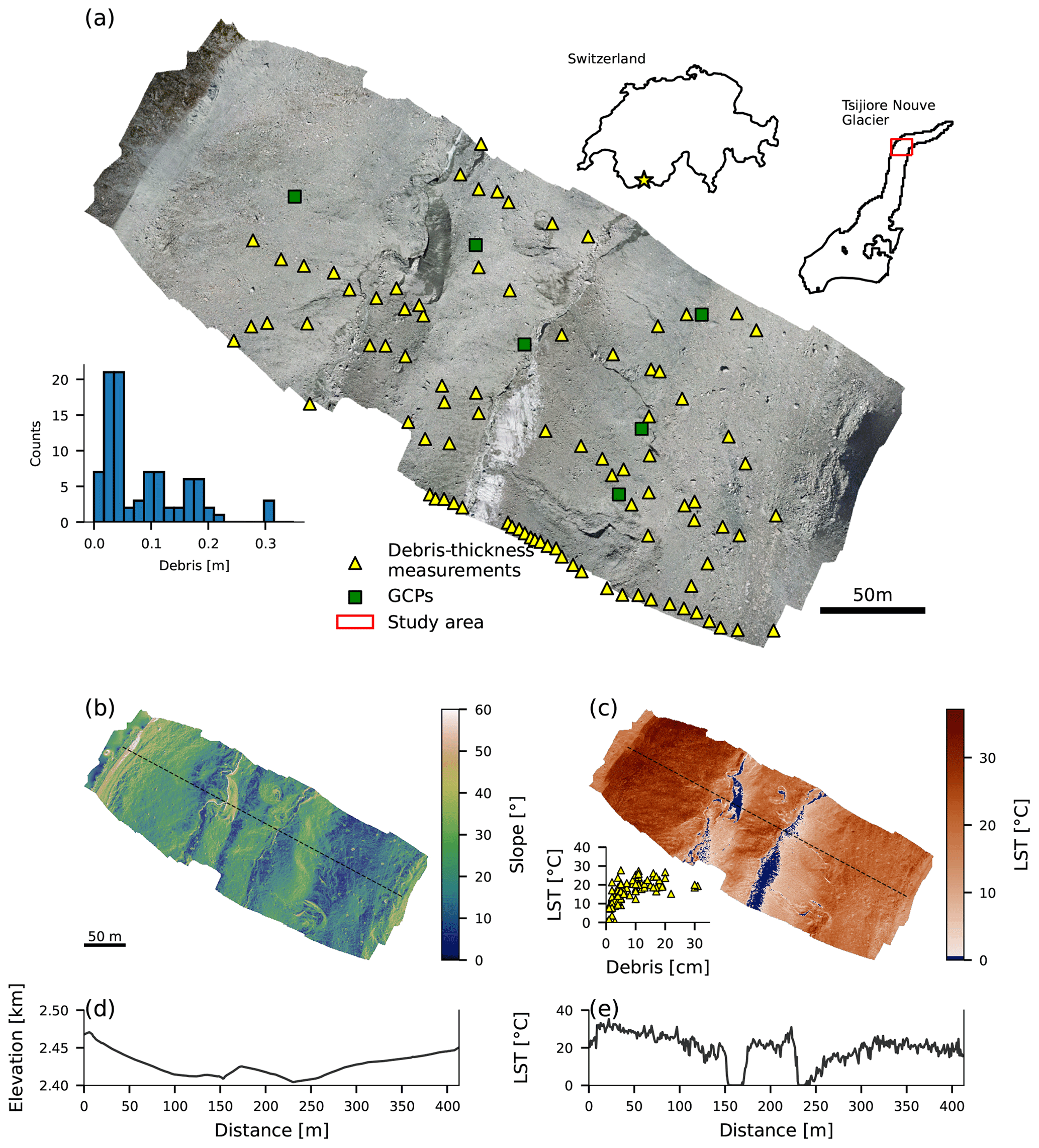
Figure 1 Overview of the study area on the Tsijiore Nouve Glacier, Switzerland. (a) Orthomosaic from optical unpiloted aerial vehicle (UAV) data obtained on 30 August 2019. Yellow triangles indicate locations of debris-thickness measurements, and green squares indicate ground control points (GCPs). The histogram shows the distribution of the debris thicknesses measured in the field. (b) Slope map obtained from UAV-derived digital elevation model (15 cm resolution). (c) UAV-derived land surface temperature (LST) at 13:00 (UTC+1). Blue areas depict LST<0.5 ^∘C. The inset scatterplot shows in situ debris-thickness measurements versus LSTs. Black dashed lines in (b) and (c) indicate profiles shown in (d) (elevation) and (e) (LST).

3 Materials and methods

3.1 Field data

Field data were collected on 30 August 2019 on an area of approximately 60 000 m² (Fig. 1a), under blue-sky conditions (isolated clouds in the late afternoon). Spatially distributed debris surface temperature was measured between 09:00 and 22:00 local time (UTC+1; hereafter we always refer to local time in the text) at 2 h intervals to capture the diurnal temperature cycle. Temperature measurements were done using a radiometric uncooled microbolometer (FLIR Tau 2 longwave infrared thermal camera) mounted to a DJI Mavic Pro UAV. The UAV followed the same pre-defined path for all eight flights at 80 m elevation above the glacier surface (terrain adjusted). Optical UAV imagery (12 MP) was recorded simultaneously with the thermal images. The thermal sensor operates within a temperature range of −40 to 160 ^∘C; has a resolution of 640×512 pixels, which, given the flight altitude, yields a thermal image resolution of approximately 0.17 m × 0.16 m; and measures longwave radiation within a range of 7.5 to 13.5 µm. Recording of the thermal infrared images was done in conjunction with the ThermalCapture 2.0 OEM (TeAx Technology GmbH), allowing for the storage of images on an SD card. The recording was done with a reduced frame rate (default 9 Hz). Each flight took between 12 and 15 min and captured around 600 thermal images. The setup is suitable for high-mountain UAV applications due to its very low size and weight. Prior to the UAV flights six ground control points (GCPs) were distributed across the area of interest (Fig. 1a). The GCPs were made from aluminum foil to be clearly recognizable in the thermal images due to the very low emissivity.

Debris-thickness measurements were made at 90 locations within the study area (Fig. 1). Coordinates of measurement locations were documented using a Garmin handheld GPS device (horizontal accuracy: ±3.6 m). The debris cover on the TNG is generally thin: measured thicknesses are below 30 cm, with a mean of 9 cm, a median of 5 cm, and a standard deviation of 10 cm. The debris cover close to lateral moraines consists of very large boulders (>0.5 m) that rendered measurements impractical and thus introduced a bias on the point measurements. Furthermore, it was not entirely clear where debris-covered ice transitioned to lateral moraines near the glacier margin.

3.2 Thermal drift and offset correction

Uncooled microbolometers are sensitive to environmental temperature fluctuations (Heinemann et al., 2020). Specifically, the sensor's detector focal plane array, the sensor housing, and the lens of uncooled microbolometers are sensitive to temperature changes. Accurate radiometric temperature measurements require a thermal equilibrium between the sensor's components and the environment. Unbalanced thermal conditions (e.g., the sensor cools down after UAV takeoff, changing wind conditions, or heats up by direct incident shortwave radiation) introduce a temperature bias. The thermal adjustment of the sensor can thus lead to changes in measurements, known as thermal drift: the recorded temperature changes, while the object's temperature remains the same (Ribeiro-Gomes et al., 2017; Malbéteau et al., 2018; Dugdale et al., 2019; Aragon et al., 2020). Furthermore, the ever-changing micro-meteorological conditions under a drone prevent the perpetuation of a thermal equilibrium and hamper accurate radiometric measurements.

The FLIR Tau 2 sensor performs an internal calibration, the flat field correction (FFC), to correct for non-uniformities by lens distortions and variations in the thermal pixel-to-pixel sensitivity. FFC is performed using the shutter at power up, when the camera changes temperature, and periodically during operation. The shutter is considered to be a uniform temperature source for each pixel and is used to update the offset correction coefficients. This internal calibration leads to in-flight temperature jumps that are accounted for in a postprocessing step, called drift compensation. The occurrence of the FFC events is used to calculate linearly backwards an offset value for each frame (TeAx; Stefan Thamke, personal communication, 2021). Usually, this is done automatically by the ThermoViewer software, but in our case, the reduced frame rate resulted in the loss of several frames containing the FFC occurrence metadata entry: a drawback of the system one should be aware of. However, we identified the frames following the internal calibration and implemented the drift compensation ourselves (Fig. 2b). To find the temperature jumps within the images, we used a threshold of 2 K differences in the mean temperature of the overlapping part in consecutive image pairs. The temperature jumps are clearly visible in the histogram time series (Fig. 2a), and we found this threshold to match the temperature jumps best. The overlap was defined as the bounding box of matching keypoints detected in successive images using the Oriented FAST and Rotated BRIEF (ORB) algorithm (Rublee et al., 2011) implemented in the scikit-image Python library (Van der Walt et al., 2014).

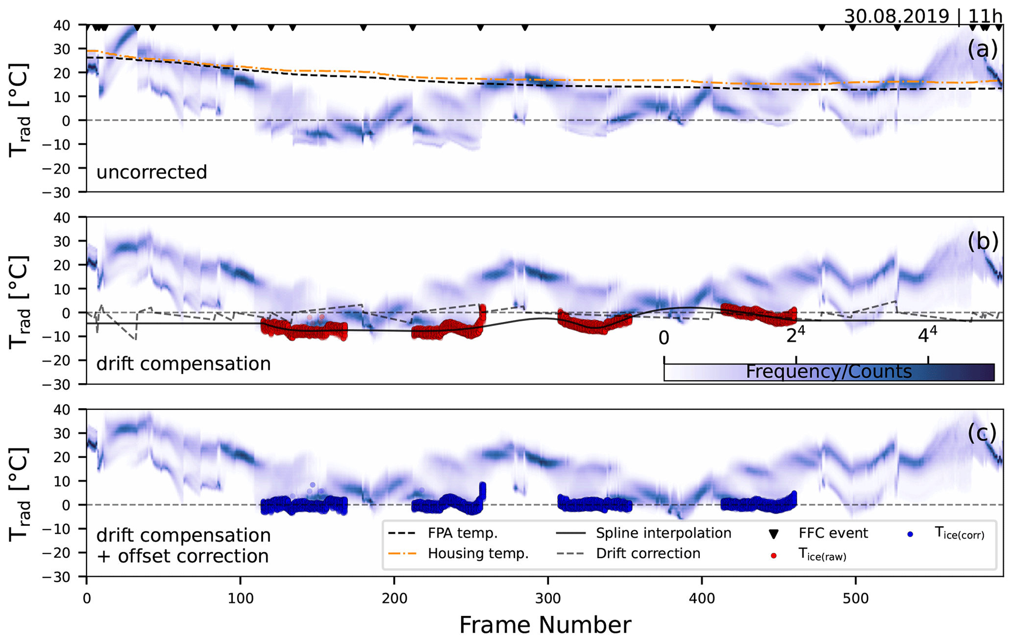
Figure 2 Thermal correction and calibration using bare-ice temperatures at 11:00 (UTC+1) on 30 August 2019. The histogram time series in the figure displays the frequency of measured temperatures in each thermal infrared image, with each vertical stripe representing one image. (a) Raw at-sensor (brightness) temperature with detected flat field correction events (black triangles). The temperatures of the focal plane array (FPA) and housing case returned by the sensor are shown in orange and a bold, dashed black line. (b) Drift-compensated temperatures with ice surface temperatures (red dots) and thermal drift correction offset (dashed line). The black line shows the spline interpolation of the measured ice surface temperatures with the edges set to a constant value. (c) Offset-corrected temperatures, each frame based on the spline interpolation that the ice surface temperatures are at 0 ^∘C.

Despite the successful detection of FFC events and applied drift compensation during postprocessing of the temperature data, we still observed bare-ice surfaces with considerable temperature deviations from 0 ^∘C, the expected temperature for a melting ice surface. Furthermore, the remaining temperature bias appears to be not constant with time (Fig. 2b). Therefore, we applied a further calibration step that employs the ice surface as a reference. The air temperature during the day of measurements was well above 0 ^∘C, and the ice surface, where visible, was melting. Therefore we assume the LST of the ice surface to be at 0 ^∘C. The extraction of the ice surface was done by a color-based segmentation algorithm using k-means clustering (Pedregosa et al., 2011) and subsequently manually confirmed, similar to the approach of Aubry-Wake et al. (2015). We then interpolated the ice temperatures using splines and calculated an offset correction for each frame, in a manner that the LST of the ice will be 0 ^∘C (Fig. 2c). The drift and offset were similar for most flights, but the evening flights showed less variation in the ice temperatures. However, for large ice temperature variations, the spline interpolation may not capture the temperature offset as shown in Fig. 2c (frame ∼ 250). The correction and calibration procedure was applied for each flight.

3.3 Orthomosaic generation (photogrammetry)

Each flight yielded around 600 thermal infrared frames (Fig. 2), of which around 400 have been used to generate orthomosaic maps, and 200 were omitted as they recorded the takeoff and landing of the UAV. The diurnal variation of the surface temperature and relatively low contrast of thermal images led to spatiotemporal variations in the reconstruction of the 3D point clouds. Instead of additional point cloud alignment (Rusinkiewicz and Levoy, 2001), we orthorectified the thermal images using the same digital surface model (DSM) obtained from simultaneously recorded optical images. Therefore, we identified and marked all GCPs in both the optical and thermal images prior to the photogrammetric processing to improve the image alignment and the calculation of the camera calibration parameters (Cook, 2017). As the footprint of the images is relatively large with respect to our area of interest, the six GCPs were visible in almost all thermal images. The generated DSM from the optical images was then used as the basis for the thermal image orthorectification. The overlapping parts were reduced by a weighted average during the orthomosaic generation. Agisoft Metashape software offers several options on how to handle overlap areas, and we found the default setting to produce the most reasonable results.

3.4 Land surface temperature (LST)

The temperature measured by the sensor, the brightness temperature, is influenced by (1) the upward-directed path radiance, (2) the radiation emitted by the surface towards the sensor, and (3) the reflected portion of the incoming atmospheric longwave radiation. Due to the low flight elevation of 80 m aboveground we neglect the path radiance. The reflected portion of incoming atmospheric longwave radiation (3) was taken from the downward thermal flux of ERA5-Land hourly reanalysis data (Muñoz Sabater, 2019) with respect to the time of flight. The large footprint of the reanalysis data (0.1^∘ × 0.1^∘) compared to the small test site (∼ 150 m × 350 m) might introduce additional uncertainties. However, the influence on the LSTs is small, as the magnitude of the reflected radiation is also very small. The retrieval of the LSTs (2) is then a function of the emissivity of the surface material and the atmospheric transmissivity between the ground and the sensor. We assume the transmissivity to be negligible under the meteorological conditions and flight altitude (Kraaijenbrink et al., 2018; Malbéteau et al., 2018). Following Stefan–Boltzmann's law we calculated the LSTs using

$$\begin{array}{}\text{(1)}& \mathrm{LST}=\sqrt[\mathrm{4}]{{\displaystyle \frac{\mathit{\sigma }{T}_{\mathrm{rad}}^{\mathrm{4}}-\left(\mathrm{1}-\mathit{\epsilon }\right)\cdot \mathrm{LW}\downarrow }{\mathit{\sigma }\mathit{\epsilon }}}},\end{array}$$

where σ is the Stefan–Boltzmann constant (5.67×10⁸ W m⁻² K⁻⁴), ε the emissivity of the surface type (debris = 0.94, rough ice = 0.97) (Rounce and McKinney, 2014; Aubry-Wake et al., 2015), and LW↓ the incoming longwave radiation (W m⁻²). Some authors point out the relevance of atmospheric transmissivity (Torres-Rua, 2017; Herreid, 2021), while others neglect it due to low UAV flight elevations above the ground surface (Sullivan et al., 2007; Hill-Butler, 2014). We think radiation attenuated by water vapor in the atmosphere between the sensor and ground would be spatially uniform and thus compensated by our calibration procedure. To assign emissivity values across the glacier surface, we distinguished between ice and debris using a supervised random forest classification with manually created training data (Breiman, 2001). By comparison with the optical imagery and according to the algorithm's mean prediction error, we found the best classification results when the temperature differences between ice and debris were the largest, at 15:00. Data from this flight were used to classify the thermal imagery.

3.5 Surface energy balance model

Thermal energy fluxes at the earth's surface are described in the surface energy balance approach used here. For a layer of supraglacial debris, the rate of change of heat stored in the debris (ΔS) must balance all incoming and outgoing energy fluxes (all fluxes have units of W m⁻² and are positive when directed towards the debris layer):

$$\begin{array}{}\text{(2)}& \mathrm{\Delta }S=\mathrm{SW}+\mathrm{LW}+LE+H+G,\end{array}$$

where SW and LW are the net shortwave and longwave radiation fluxes, H and LE are the sensible and latent heat fluxes, and G is the conductive heat flux from the debris into the underlying ice. The parameters used in the surface energy balance are listed in Table 1.

Table 1 Parameters used in the surface energy balance model.

The net shortwave radiation is a function of the albedo and the amount of incoming solar radiation. We assumed a constant debris surface albedo of 0.3 (Rounce and McKinney, 2014; Schauwecker et al., 2015). Computation of the insolation at the time of the UAV flights was done using a Python implementation of the R package “insol” (Corripio, 2003). The model determines the solar geometry (Iqbal, 1983) and estimates the atmospheric transmissivities (Bird and Hulstrom, 1981) based on a digital elevation model, which in our case was generated from the optical UAV images. Atmospheric attenuation was calculated using the relative humidity and air temperature, from ERA5-Land hourly reanalysis data at each time of flight (Muñoz Sabater, 2019). We also accounted for cast shadows by the surrounding topography, based on a 0.5 m resolution digital elevation model with a larger footprint (Swisstopo, 2021).

Net longwave radiation results from the difference between incoming longwave radiation (LW↓) and outgoing longwave radiation (LW↑). LW↓ is the same as in Eq. (1) and based on ERA5-Land data. LW↑ is a function of the LST and the surface emissivity (see Sect. 0) and calculated following Stefan–Boltzmann's law $\mathrm{LW}\uparrow =\mathit{\epsilon }\mathit{\sigma }{\mathrm{LST}}^{\mathrm{4}}$. The latent heat flux (LE) is assumed to be 0, as the debris surfaces were dry during the UAV flights.

The sensible heat flux H was estimated using the bulk aerodynamic approach assuming a neutral atmosphere (Nicholson and Benn, 2006; Steiner et al., 2018; Nakawo and Young, 1982; Rounce and McKinney, 2014):

$$\begin{array}{}\text{(3)}& H={\mathit{\rho }}_{\mathrm{air}}{\displaystyle \frac{P}{P_{\mathrm{0}}}}{c}_{\mathrm{a}}{C}_{\mathrm{bt}}u\left(T_{\mathrm{air}}-\mathrm{LST}\right),\end{array}$$

where ρ_air is the air density at sea-level pressure (kg m⁻³); P₀ is the atmospheric pressure at sea level (Pa); P is the atmospheric pressure at site elevation (Pa), calculated following Iqbal (1983); c_a is the specific heat capacity of air (J⁻¹ kg⁻¹ K⁻¹) (Brock et al., 2010; Barry et al., 2022); u is the wind speed (m s⁻¹); T_air is the air temperature; and C_bt the bulk transfer coefficient given as

$$\begin{array}{}\text{(4)}& C_{\mathrm{bt}}={\displaystyle \frac{k_{\ast }^{\mathrm{2}}}{\ln \left(\frac{z_u}{z_{\mathrm{0}}}\right)\ln \left(\frac{z_t}{z_{\mathrm{0}}}\right)}},\end{array}$$

where k_∗ is the Kármán constant (0.41), z₀ is the surface roughness length (Rounce and McKinney, 2014; Stewart et al., 2021), and z_u and z_t are the measuring height (m) for wind speed and air temperature. The meteorological input data u and T_air were taken from ERA5-Land hourly reanalysis data (Muñoz Sabater, 2019).

The conductive heat transfer through the layer of debris and into the ice can be described by Fourier's law assuming a homogeneous layer of debris:

$$\begin{array}{}\text{(5)}& G=-k{\displaystyle \frac{\partial T}{\partial z}}\approx -k{\displaystyle \frac{\mathrm{LST}-T_{\mathrm{di}}}{d}},\end{array}$$

where $\frac{\partial T}{\partial z}$ is the temperature gradient in the debris layer and k the effective thermal conductivity (W m⁻¹ K⁻¹). We assume a linear temperature gradient in the debris layer and thus $\frac{\partial T}{\partial z}$ to be equal to the difference between the LST and the temperature of the debris–ice interface (T_di), which we assume to be at the melting point 0 ^∘C. The assumption of a linear temperature gradient applies only approximately and for thin debris thicknesses (<10 cm) (Conway and Rasmussen, 2000; Nicholson and Benn, 2006; Rounce and McKinney, 2014). The average diurnal temperature profile through a layer of debris can be considered linear, but at sub-daily time intervals, the profile varies in its degree of linearity (Reid and Brock, 2010). We come back to this point in the Discussion.

Solving the surface energy balance at sub-daily time intervals requires knowledge of the energy flux due to the change of heat stored in the layer of debris (ΔS) (Brock et al., 2010).

$$\begin{array}{}\text{(6)}& \mathrm{\Delta }S={\mathit{\rho }}_{\mathrm{d}}{c}_{\mathrm{d}}{\displaystyle \frac{\partial {\stackrel{\mathrm{‾}}{T}}_{\mathrm{d}}}{\partial t}}d,\end{array}$$

where ρ_d is the debris density (kg m⁻³), c_d the specific heat capacity of debris (J kg⁻¹ K⁻¹), d the debris thickness (m), and $\frac{\partial {\stackrel{\mathrm{‾}}{T}}_{\mathrm{d}}}{\partial t}$ the average rate of mean debris temperature change (K s⁻¹) with ${\stackrel{\mathrm{‾}}{T}}_{\mathrm{d}}$ as the mean debris temperature, $(\mathrm{LST}+T_{\mathrm{di}})/\mathrm{2}$, and t the time. Our sub-daily multitemporal LST measurements allow us to estimate temporal changes in LSTs, but these are very sensitive to uncertainties in the LST measurements (see Sect. 3.2). To avoid such issues, we rely on the diurnal temperature cycle and fitted a linearized harmonic sine function (Shumway and Stoffer, 2000) to the temperature data of each pixel. The first derivative with respect to time of this function is the warming/cooling rate and can be used to calculate the change in the heat storage term.

3.6 Debris-thickness estimation

As both the stored heat flux (ΔS) and the conductive heat flux (G) in the surface energy balance model (SEBM) are a function of the debris thickness, the surface energy balance model (Sect. 3.5) can be described by a quadratic equation in the form of

$$\begin{array}{}\text{(7)}& d^{\mathrm{2}}\left(-p_{\mathrm{d}}{c}_{\mathrm{d}}{\displaystyle \frac{\partial {\stackrel{\mathrm{‾}}{T}}_{\mathrm{d}}}{\partial t}}\right)+d\left(\mathrm{SW}+\mathrm{LW}+H\right)-k(\mathrm{LST}-T_{\mathrm{di}})=\mathrm{0}.\end{array}$$

Solving for debris thickness was done using the quadratic formula

$$\begin{array}{}\text{(8)}& d={\displaystyle \frac{-b+\sqrt{b^{\mathrm{2}}-\mathrm{4}ac}}{\mathrm{2}a}},\end{array}$$

with $a=-{\mathit{\rho }}_{\mathrm{d}}{c}_{\mathrm{d}}\frac{\partial {\stackrel{\mathrm{‾}}{T}}_{\mathrm{d}}}{\partial t}$, $b=S+L+H$, and $c=-k(\mathrm{LST}-T_{\mathrm{di}}$). Note that the quadratic equation has mathematically two solutions, whereas only one is physically plausible.

In addition to the SEBM approach, we also estimated debris thickness for each LST map using a rational curve (McCarthy, 2019; Boxall et al., 2021) of the form

$$\begin{array}{}\text{(9)}& d={\displaystyle \frac{\mathrm{LST}}{c_{\mathrm{1}}+c_{\mathrm{2}}\mathrm{LST}}},\end{array}$$

where c₁ and c₂ are empirically derived coefficients by a least squares regression.

To evaluate the performance of the two approaches for predicting debris thickness, we used the RMSE between the predicted and the observed debris thickness at the sites surveyed in the field (Sect. 3.1). To account for the accuracy of the handheld GPS device, we used the mean variable values within a 2 m radius buffered region around the GPS coordinate. Sites for which the SEBM approach did not yield a real and positive number were excluded from the comparison. We discuss the causes for these unphysical solutions in detail in Sect. 5.1. To evaluate the least squares regression of the rational curve we divided the observed debris-thickness data into a testing (n=45) and training (n=45) dataset. The training dataset has been used to derive the model coefficients c₁ and c₂, while the testing dataset was used to compare the modeled debris-thickness estimates with the field observations.

4 Results

4.1 Land surface temperature and its diurnal variation

The LST changes over the day in a cyclic manner (early morning cool – afternoon hot – evening cool), and consequently the ability to estimate debris thickness using LST changes accordingly (Fig. 3). Unlike satellite-derived LST observations, our diurnal LST measurements allow us to show how this relationship changes throughout the day.

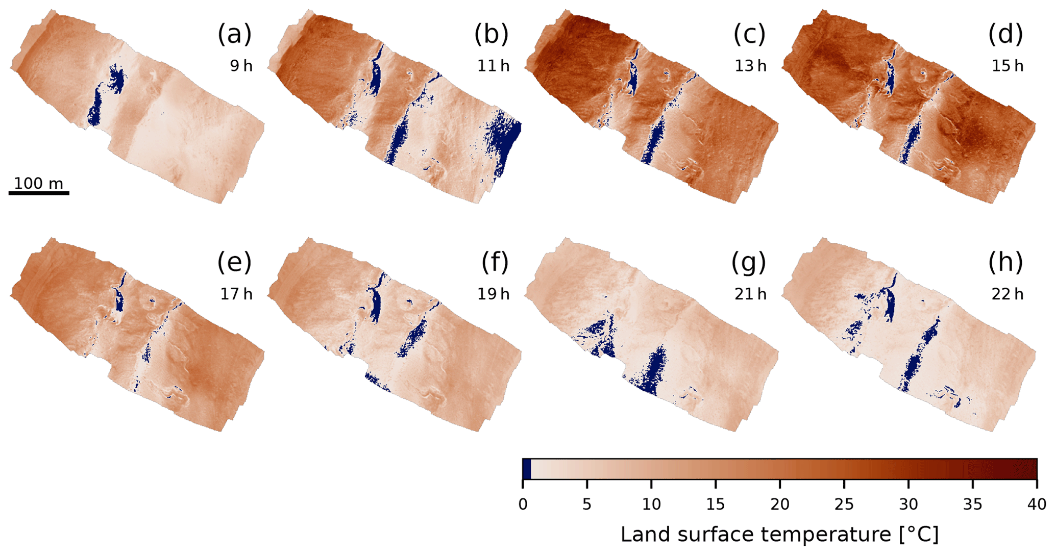
Figure 3 Spatiotemporal distribution of the land surface temperature (LST). Panels (a–h) show the eight individual flights, describing a large fraction of the diurnal land surface temperature variation. The maps have a spatial resolution of 15 cm and are colorized in dark blue for LST<0.5 ^∘C. Due to the residual uncertainties of the LSTs, ice surface geometries appear inconsistent with time. The southeast region of panel (b) (11:00 UTC+1) shows an unreasonable cold temperature due to a failed calibration.

LST and debris thickness are generally positively correlated, but the suitability of a linear model to describe the relationship varies throughout the day with better correlation for cooler temperatures in the evening hours (Fig. 4f–h). In the afternoon hours when the debris surface reaches its maximum diurnal temperature, the relationship between debris thickness and LST shows its non-linear nature (Fig. 4c–e). Additionally, we observe the influence of the terrain aspect: east- and south-facing slopes heat up earlier compared to west- and north-facing slopes (Fig. 4a, b) (Crameri et al., 2020).

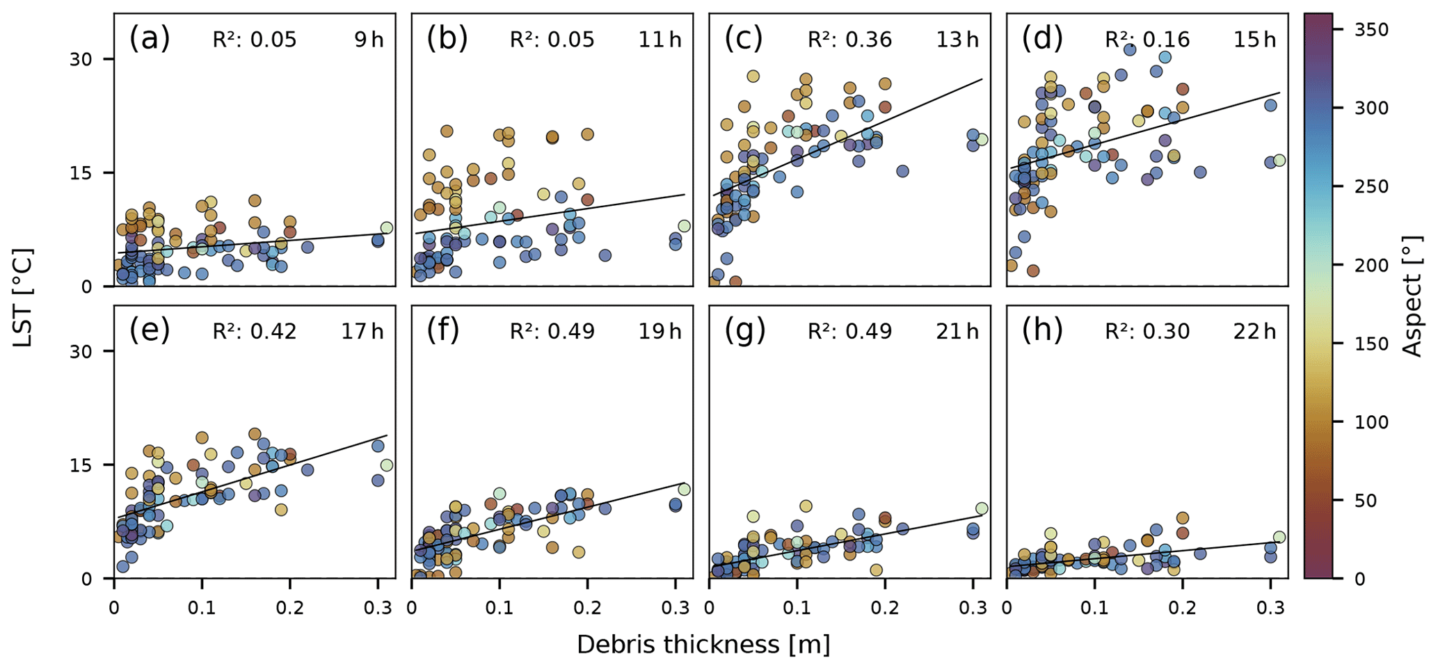
Figure 4 The temporal variation of the land surface temperature (LST) against in situ-measured debris thickness. Panels (a–h) show the arithmetic mean land surface temperature of a 2 m buffered region around the GPS coordinates of debris-thickness measurements colorized for terrain aspect with $\mathrm{0}/\mathrm{360}$^∘ facing north. The LST of the warming phases (a–d) is more strongly influenced by the aspect than the cooling phases (e–h). The non-linear nature of the relationship between the LST and debris thickness is noticeably pronounced for higher LSTs (c–e), while the correlation for low LSTs appears more linear (f–h).

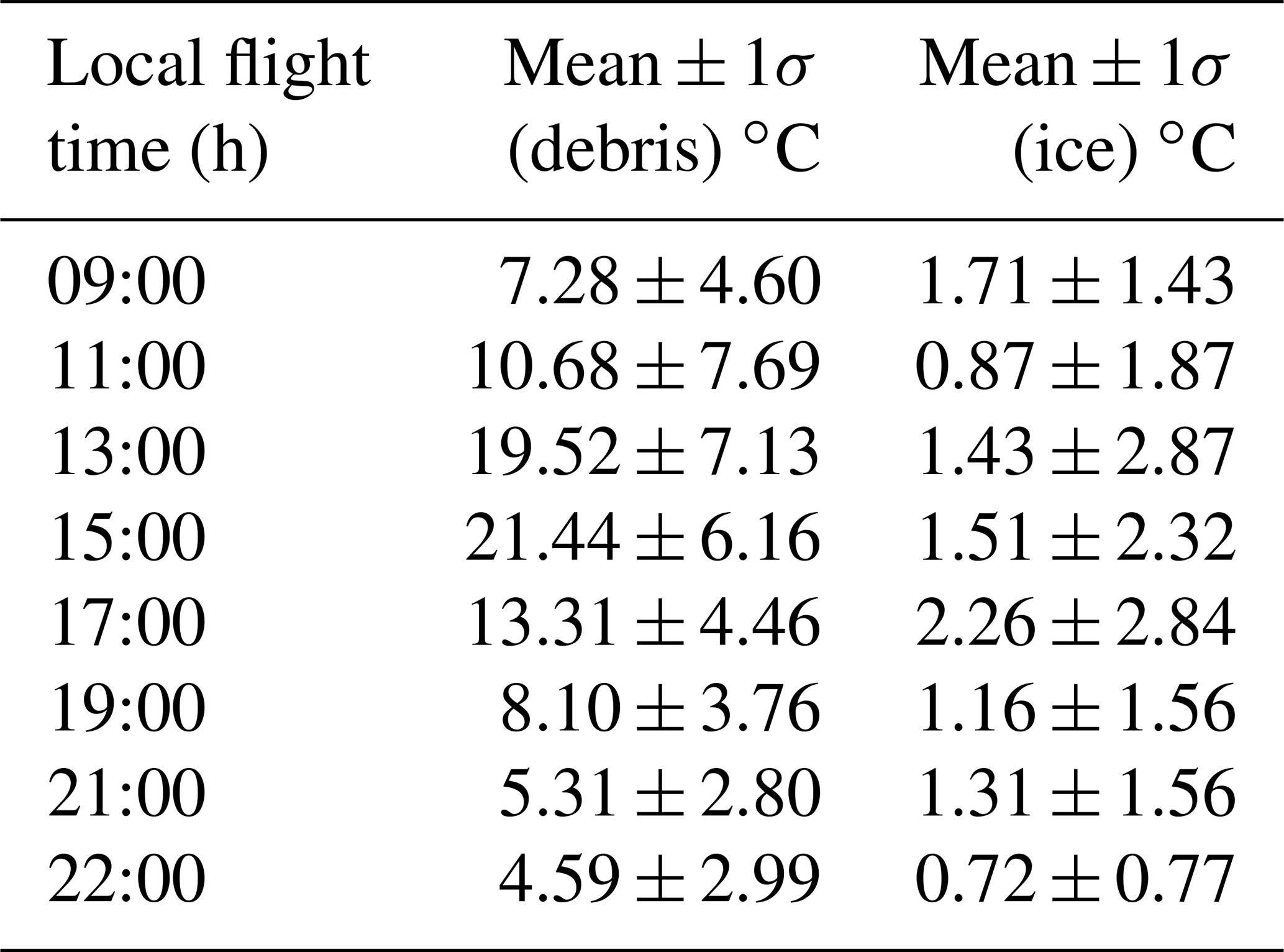
The effect of the terrain aspect is not evident during the cooling phase in the afternoon and evening. The spatial and temporal variability of the LSTs (Fig. 3) shows that at all flight times, surface temperatures are higher at the edges of the glacier (NW and SE) and lower in the central part of the test area. This pattern corresponds to high debris thicknesses at the glacier margins and thin debris thicknesses or no debris occurrence in the middle part. The mean LST of the debris cover follows the expected pathway of a diurnal temperature cycle (Table 2).

Table 2 Mean LST and standard deviation (1σ) of the debris and ice surface type.

While the general spatial and temporal pattern of LSTs seems to be reasonable, some areas of concern exist locally. First, the southeastern region of the 11:00 flight shows an unreasonable cold temperature patch, which most likely does not represent the actual LST at that time. Instead, we suspect that this artifact corresponds to an uncorrected bias of the thermal correction and calibration process. We come back to this point in the Discussion. Second, the 15:00 flight shows a centrally located, transverse-oriented strip of higher LSTs, which seems to follow the flight path of the UAV. The directional temperature mismatch could be related to an oblique viewing angle of the sensor, as the nadir alignment was set up manually, and the angle of observation might partly control the amount of radiation received by the sensor and thus the temperature measurement (Norman and Becker, 1995).

In the absence of any other means to assess the precision of the LST values, we suggest that the variability of the bare-ice surface temperatures, which ought to be at 0 ^∘C, might indicate the bias and precision of the LSTs. The LST values of ice surface temperatures vary by several degrees with a standard deviation of up to 2.87 ^∘C (Table 2). Mean ice LSTs range between 0.72 and 2.26 ^∘C throughout the day (Table 2). Field observations show that ice cliffs on the TNG are often sprinkled with small rocks and/or a thin layer of dust, which might influence the ice LSTs towards warmer temperatures.

Based on the LST measurements, we estimated the diurnal variation of the depth-integrated mean debris temperature. The pixel-wise fitted harmonic sine functions allow us to estimate the spatially distributed warming and cooling rates, as the first derivative with respect to time. The RMSE of the fit (mean±1σ) is 1.51±0.54 ^∘C. The spatial distribution of the RMSE (Fig. 5b) is relatively continuous but shows variability where the before-mentioned local LST discrepancies occur. Figure 5a shows that, depending on the aspect, at 13:00 and 15:00 the debris surface reaches its maximum LST, and consequently the temperature change rate converges to zero.

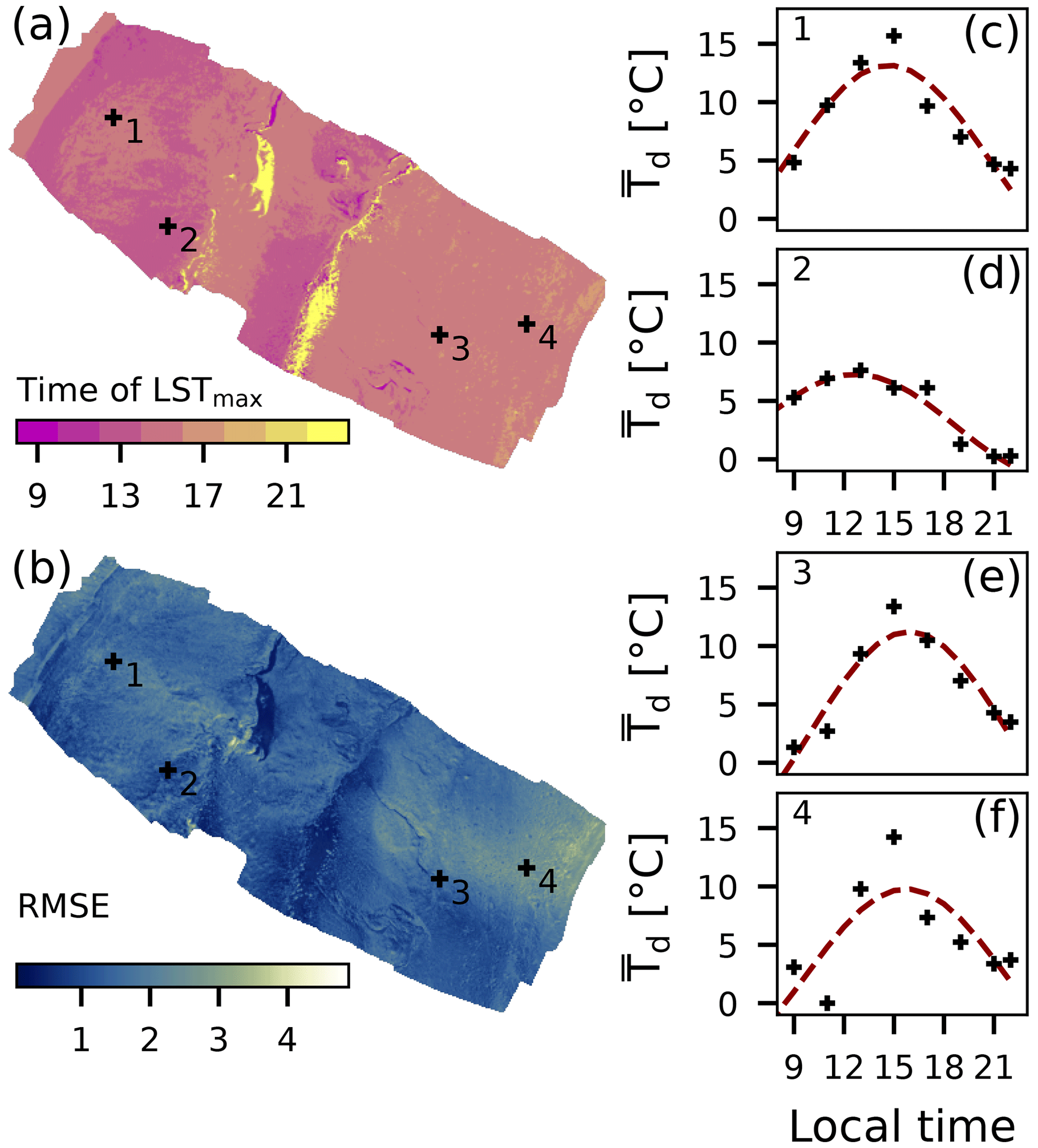
Figure 5 Sinusoidal regression of mean debris temperature (${\stackrel{\mathrm{‾}}{T}}_{\mathrm{d}}$), estimated from LSTs (Eq. 6) for each pixel. (a) The panel shows the time at which ${\stackrel{\mathrm{‾}}{T}}_{\mathrm{d}}$ reaches its maximum diurnal temperature and thereby emphasizes the effect terrain aspect. (b) The RMSE of the regression for each pixel. The southeastern region with larger errors is due to the anomalies in the LST at 11:00 (UTC+1); see the text for details. The spatial mean of the RMSE is 1.51 ^∘C, and the standard deviation is 0.54 ^∘C. The panels (c–f) are example points of the sine function used to derive the warming/cooling rate in each pixel. Locations of the examples are indicated in panels (a) and (b).

4.2 Surface energy balance modeling

To solve the surface energy balance (Eq. 2) we determined the LST-independent energy flux component SW and the LST-dependent components LW, H, ΔS, and G, based on the UAV-derived LST maps shown in Fig. 3. In Fig. 6, we show the diurnal variation of each component, evaluated at all locations where we obtained debris-thickness measurements.

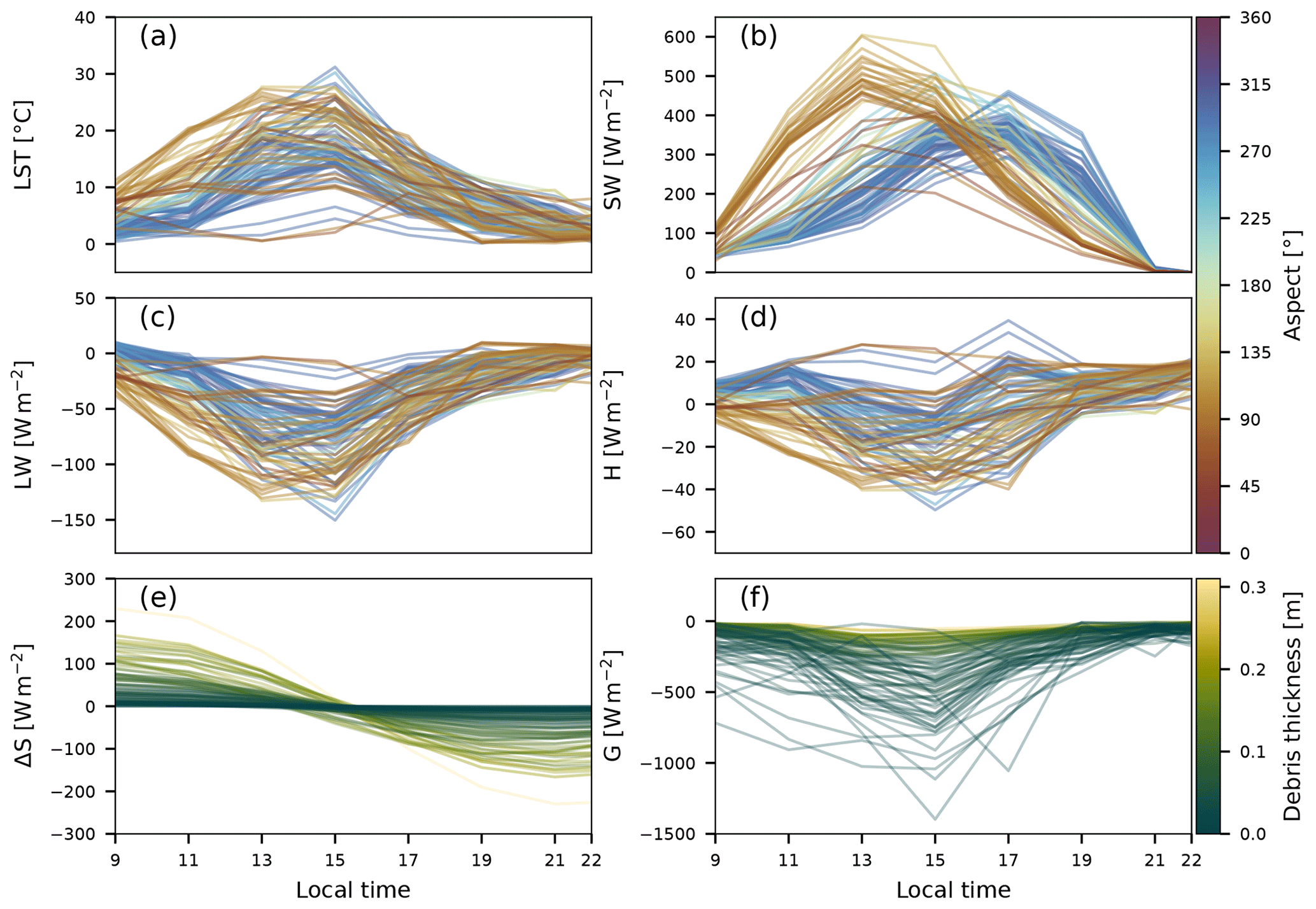
Figure 6 Energy fluxes at debris-thickness measurement locations. Diurnal variations of (a) land surface temperature, LST; (b) net shortwave radiation, SW; (c) net longwave radiation, LW,; and (d) sensible heat flux, H, with lines colorized by terrain aspect with $\mathrm{0}/\mathrm{360}$^∘ facing north. Diurnal variations of (e) the change in heat storage, ΔS, and (f) the conductive heat flux, G, with lines colorized by debris thickness measured in the field. Note that only SW (b) is independent of LSTs, whereas data in panels (c–f) are a function of LSTs.

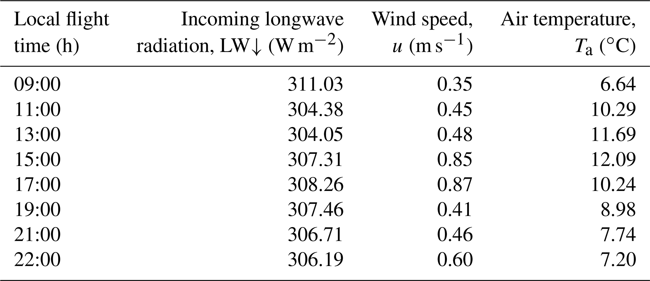
East- and south-facing slopes receive their maximum net shortwave radiation (SW) prior to the west- and north-facing slopes (Fig. 6b), which explains their earlier increase in LSTs (Fig. 6a). By 15:00, all sites attained the daily maximum LST and cool down from then on. Despite the remaining differences in SW, no more aspect-related differences in LSTs can be observed. All the remaining SEBM components are a function of the LSTs and thus also show an aspect dependency before 15:00. The net longwave component (LW) expectedly mirrors the LSTs (Fig. 6c). The sensible heat flux (H), calculated using the bulk approach (Eq. 3), attains only low flux values close to 0, which is likely related to the low wind velocities (<1 m s⁻¹) obtained from reanalysis data (Table 3). The rate of change in heat storage within the debris (ΔS) and the conductive heat flux (G) are, besides the LSTs, a function of the debris thickness (Eq. 6, Fig. 6e, f). Whereas ΔS attains the largest magnitudes in the morning and evening hours and where the debris is thick, the opposite is true for G, which is largest at 15:00 and where the debris is thin.

Table 3 ERA5-Land hourly reanalysis data on 30 August 2019 interpolated at the Tsijiore Nouve Glacier, Switzerland (46.01^∘ N, 7.46^∘ E).

4.3 Debris-thickness estimates from SEBM

The SEBM-derived predictions of debris thickness (Fig. 7) show a general pattern that matches observations in the field and the pattern of measured LSTs. Predicted debris thicknesses generally range between 0 and 30 cm. Given the chosen input parameters, Eq. (8) cannot be solved for all pixels in the first half of the day (09:00 to 15:00) (Fig. 7a–d).

Figure 7 Estimated debris thicknesses for each flight time. White regions show regions where the surface energy balance model has no valid solution for debris thickness due to high uncertainties in the land surface temperature and reanalysis data. The histograms show the distribution of the predicted debris thicknesses displayed in the maps.

At these times the quantities of the surface energy balance components and the relatively low LSTs lead to a negative term under the root in Eq. (8) and thus to no valid solution. Predictions of thicker (>10 cm) debris are primarily found in the afternoon and evening hours (17:00 to 22:00), and the pattern of thin debris (<10 cm) predictions, primarily in the central part of the glacier, is relatively consistent in time.

Comparing the predictions to field observations (Fig. 8) shows that the accuracy of the prediction remains comparable throughout the day with an RMSE of 6 to 8 cm. For most of the flights, we find a positive correlation between the predictions and observations, even if they do not follow the 1:1 line. During the warming phase of the day, when the aspect has a strong influence on LSTs (Fig. 4a–c), the associated debris predictions do not show an aspect-related pattern. In contrast, debris-thickness predictions based on the afternoon flights at 17:00 and 19:00 seem to correlate with aspect whereas the LST data do not.

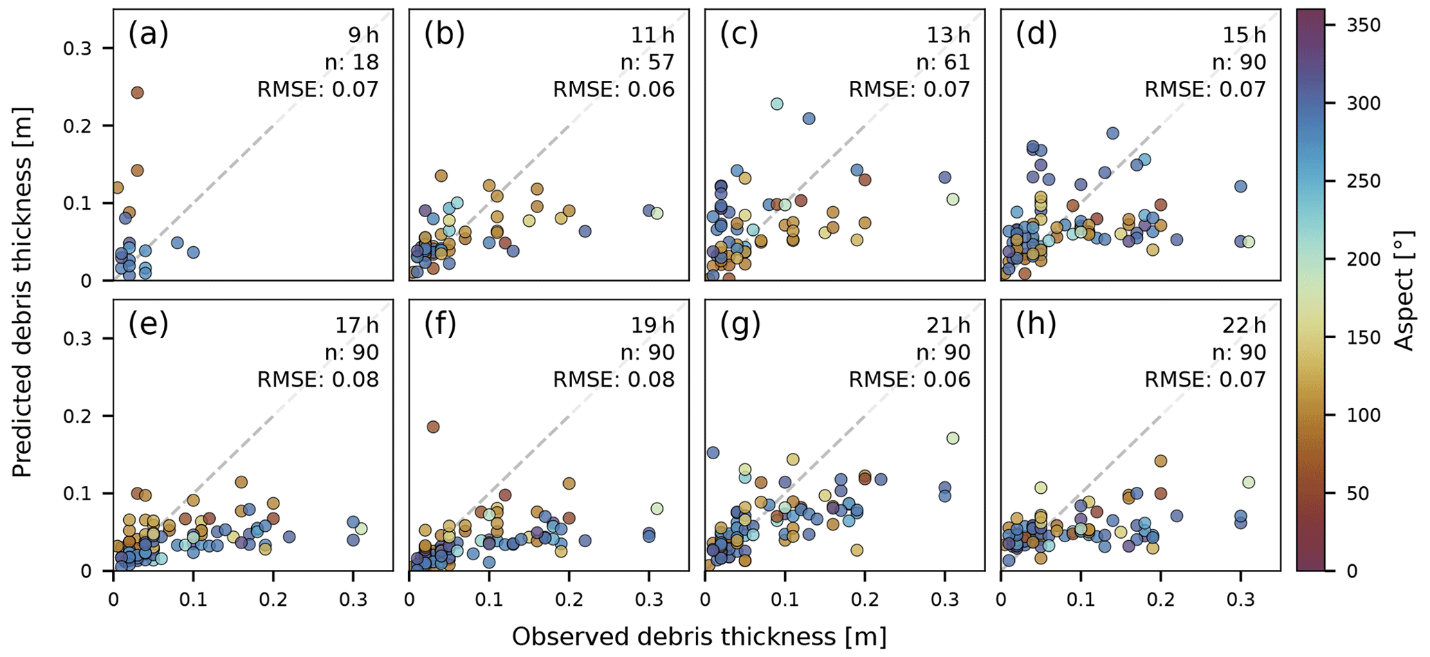
Figure 8 Comparison of modeled and observed debris thickness for each flight time (a–h) with RMSE values (m) for model evaluation. Sample points are colorized by terrain aspect and the dashed grey line shows the 1:1 line. RMSE for flights (a, b, c) is based on a reduced sample number.

Absolute values of predicted thin debris cover are less sensitive to the time of the day, compared to thick debris. Figure 9a shows the variation of the predicted thicknesses with time along the profile introduced in Fig. 1b as the mean value ±1σ. The spatial variability of the standard deviation is shown in Fig. 9d. As the SEBM does not yield a valid solution for all times of the day, Fig. 9e additionally shows the number of valid predictions in time. Towards the glacier edges where the debris is greater than 10 cm, the spread in the standard deviation increases, compared to the central part, showing that the prediction of thick debris cover varies stronger in time than for thin debris cover.

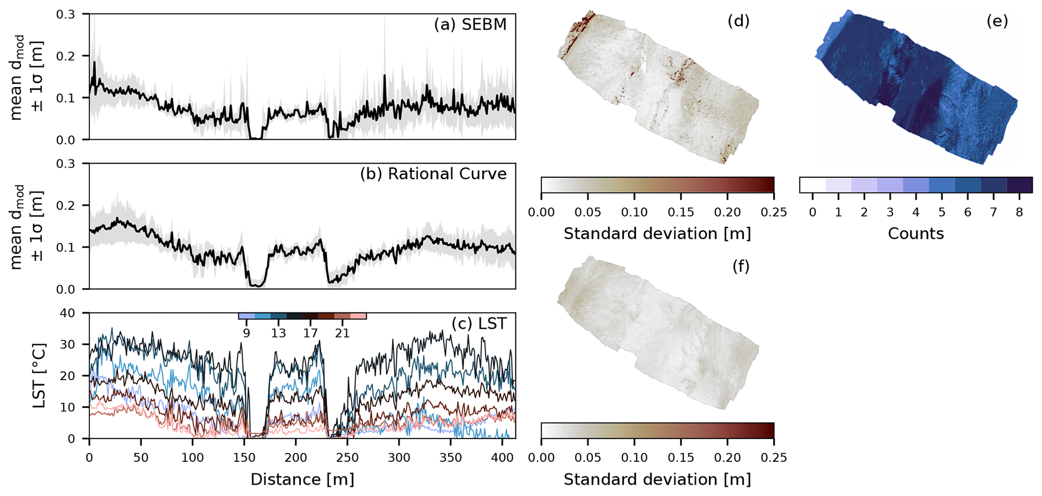
Figure 9 Diurnal mean ± 1σ debris-thickness predictions along the profile line shown in Fig. 1. (a) The predictions using the surface energy balance model (SEBM) show a larger spread of the standard deviation (grey) towards the edges and smaller towards the central part corresponding to regions of thicker and thinner debris cover. Panel (b) shows the results of the rational curve extrapolation approach. A smaller spread indicates greater consistency in the prediction over the day. (c) The diurnal variability of the land surface temperature along the profile line. Panels (d, f) show the spatial variation of the standard deviation and (e) the number of valid solutions in the SEBM approach.

4.4 Debris-thickness estimates by extrapolating a rational curve

The debris-thickness maps created by the extrapolation approach using a rational curve result in slightly thicker predictions than following the SEBM approach (Fig. 10). The general pattern of the spatial debris-thickness distribution follows the field observations and the pattern of measured LSTs, similar to the results of the SEBM approach. The modeled debris thicknesses vary between 0 and 30 cm but with early flights at 09:00 and 11:00 lacking predictions greater than 10 cm (Fig. 10a, b).

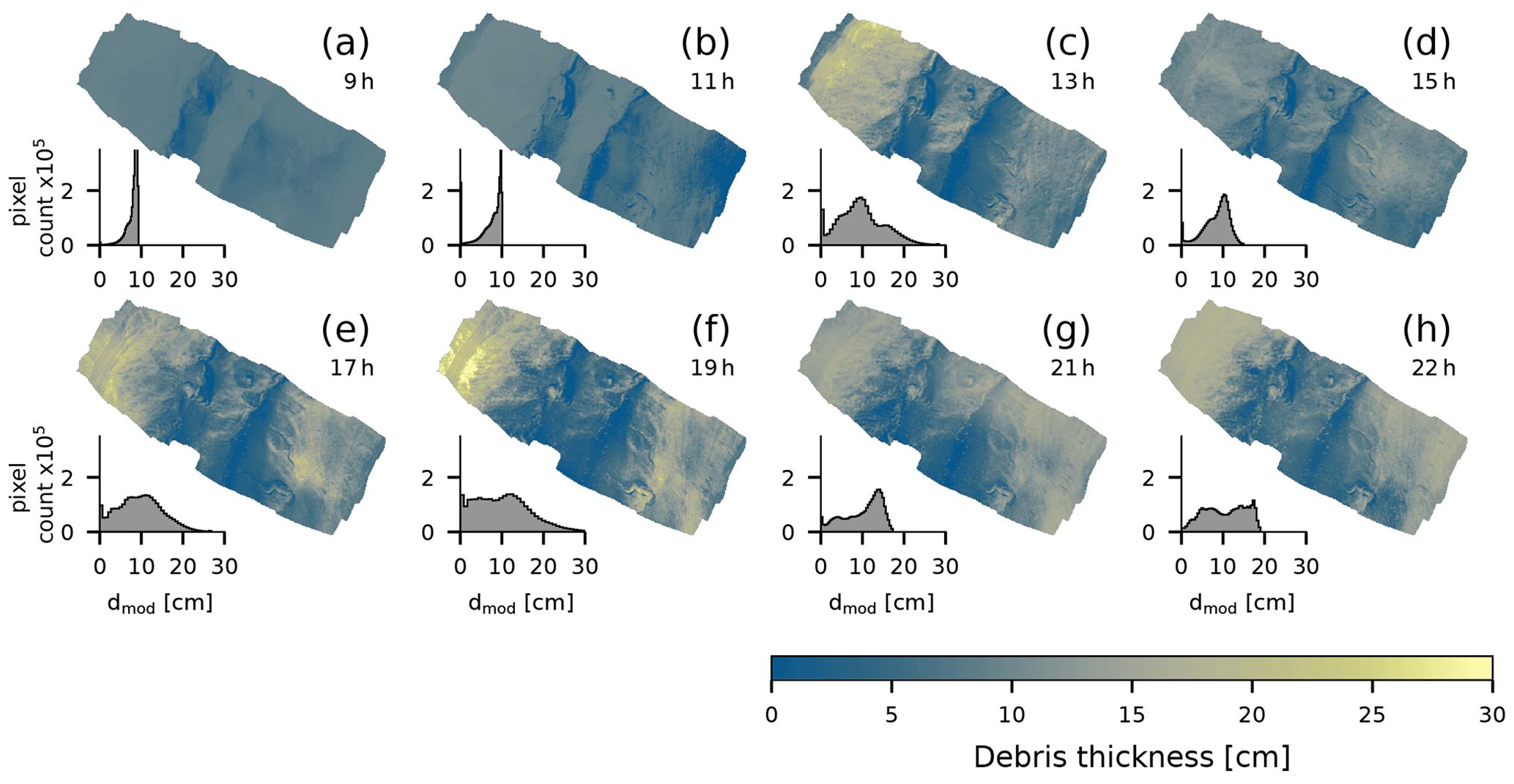
Figure 10 Estimated debris thickness using a rational function for each flight time. The histograms show the distribution of the predicted debris thicknesses displayed in the maps.

We divided (Pedregosa et al., 2011) the dataset of n=90 samples into a training (n=45) and testing (n=45) dataset. Figure 11 shows training and testing data for each flight time, including the coefficients c₁ and c₂, derived by least squares regression of Eq. (9) and the RMSE between the predictions and the observations of the testing data (Fig. 11). Similar to the SEBM, the RMSE ranges between 6 and 8 cm, but debris thicknesses >10 cm are better represented in the extrapolation approach and thus follow more closely the 1:1 line. At 09:00, 11:00, and 15:00 the RMSE is highest at 8 cm, and the shape of the curve already shows that the model does not represent the data well. The aspect dependency of the LSTs at these times (Fig. 4a, b) was not considered as an additional parameter for the regression and thus results in a curve that does not represent the shape of the data well (Fig. 11a, b). The afternoon flights between 17:00 and 22:00 have the lowest RMSE with 6–7 cm.

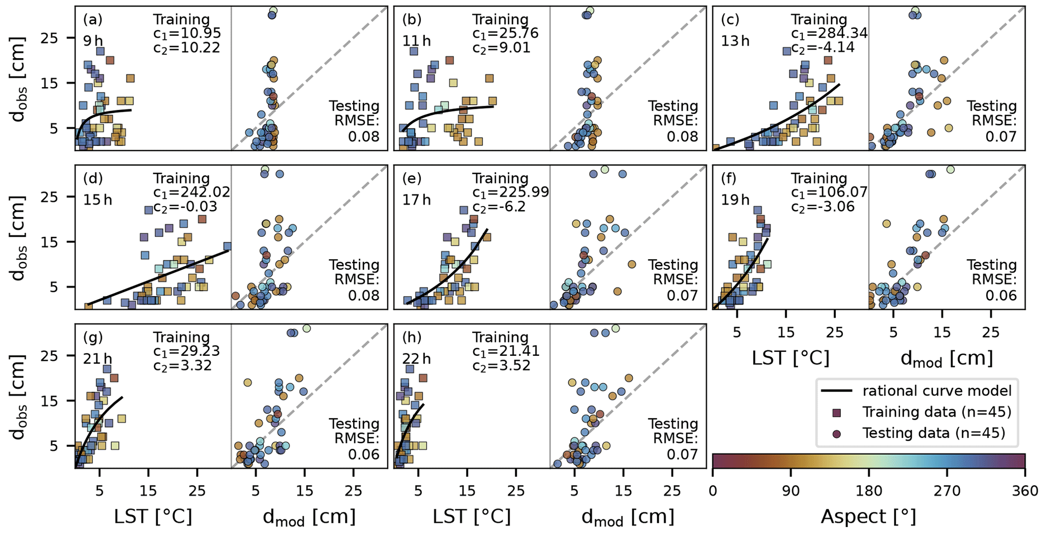
Figure 11 Least squares regression of a rational function of 50 % of the debris-thickness measurements (n=45) with the arithmetic mean land surface temperature of a 2 m buffered region around the GPS coordinates of debris-thickness measurement locations (training data) (a–h). The adjacent panels show the comparison of modeled and observed debris thickness of the other 50 % (n=45) with RMSE values to evaluate the prediction (testing data). Sample points are colorized by terrain aspect.

The diurnal stability in predicting debris thickness (Fig. 9; diurnal mean ± 1σ debris-thickness predictions along the profile line shown in Fig. 9f) shows that thin debris cover, as found in the central part of the profile line, remains stable throughout the day and is thus comparable to the results of the SEBM approach. For thicker debris the spread of the standard deviation is higher, showing that predicting thick debris cover depends more on the time of the day than thin debris. Even though the range of the RMSE throughout the day remains comparable to the SEBM results, for some flights (e.g., 19:00) the average prediction accuracy improves by about 2 cm.

5 Discussion

5.1 Predicted versus observed debris thickness

Debris-thickness predictions with the SEBM approach yielded mixed results. The fact that the modeled debris thickness does not vary in unreasonable ways across the glacier surface, but in a systematic pattern, shows that mapping high-resolution debris thickness with UAVs has some potential. During most of the flights, we observe a general positive correlation between the modeled and observed debris thickness (Fig. 8b–h). The overall relationship between higher surface temperature and thicker debris that is evident in the input data (Fig. 4) can be reproduced. However, given the chosen parameters, we are unable to obtain a non-biased match between the observed and modeled debris thickness. The SEBM approach mostly underestimates debris thickness at all flight times compared to field measurements. For thick debris cover, this underestimation is more pronounced than for thin debris (<10 cm).

Over the course of the day, the RMSEs between observed and predicted debris thicknesses range from 6 to 8 cm. For many pixels in the flights at 09:00, 11:00, and 13:00 and some pixels at 15:00 (Fig. 7a–d) the quadratic equation (Eq. 7) has no real solution, and the SEB cannot be solved for debris thickness. The reason for this is a negative term in the square root of Eq. (8), which occurs if b²<4ac. Recall that b accounts for the radiative and sensible heat fluxes (SW + LW +H), whereas a and c are the conductive heat flux and the storage term, respectively. As long as LST>0 ^∘C, c is always negative. The inequality condition above can thus only occur if also a is negative, which is only possible when the debris is heating up, in our case until about 15:00 (Figs. 5a, 6e). That explains why many pixels in the morning flights have no debris-thickness solution. Furthermore, at 09:00, the term b² is rather small, mostly because of low SW values. However, at 11:00 and 13:00 southeast-exposed pixels receive higher SW (Fig. 6b), which causes b to increase, making the inequality condition less likely. The most likely reason for no physical solution to Eq. (7) is inaccurate values of LSTs and reanalysis-derived variables. Mostly during the morning, even small deviations from true values are sufficient to find no physically meaningful debris-thickness solution. For thin debris (<2 cm), G is very sensitive to uncertainties in LSTs and leads to large negative numbers. This is a major drawback of the SEB approach, and it highlights the sensitivity of the approach to uncertainties in the input data. We note that these uncertainties prevail, even if a solution is found. However, compared to the ground observations of debris thickness the model predictions show a positive correlation.

As a result of spatially incomplete debris-thickness maps, the number of sample points to evaluate the quality of the prediction is reduced (see low n in Fig. 8a–c) and should be kept in mind when comparing the RMSE with respect to the time of the day. Previous studies did not face this issue, in part because ΔS was incorporated as a fraction of the conductive heat flux G, which is always negative (Foster et al., 2012; Schauwecker et al., 2015). Comparison of ΔS and G for the sites where we measured debris thickness shows that such an assumption appears to be invalid for most times of the day (Fig. 5). By estimating ΔS using the warming/cooling rate from multitemporal LST measurements, we can better account for this energy balance component, but these estimates are also prone to uncertainties in LSTs. In general, however, the magnitude and distribution of SW, LW, and ΔS for most of the sample locations compare well to values determined by Brock et al. (2010) with an automatic weather station (AWS) at the Miage Glacier at comparable latitude, time of the year, and elevation (500 m difference).

Debris-thickness predictions below ∼ 10 cm seem to correlate reasonably well with field observations, whereas predictions of thicker debris cover are generally too low (Fig. 8). This may indicate that uncertainties in parameters that are unlikely to vary spatially or as a function of debris thickness are not particularly relevant. To further test this hypothesis, we performed sensitivity tests of SEBM-derived debris-thickness estimates to variations in the input parameters air temperature, wind speed, thermal conductivity, albedo, and surface roughness length (Fig. 12). Variations of the parameters air temperature, albedo, and surface roughness length across value ranges commonly found in the literature (Brock et al., 2000; Foster et al., 2012; Schauwecker et al., 2015; Shaw et al., 2016; Miles et al., 2017) result in generally small variations of the mean debris thickness (averaged across the entire studied surface). In consequence, the impact on the RMSE when evaluated against our field observations of debris thickness is also small. Only the flights at 09:00, 11:00, and 13:00 show more significant variations in the RMSE, but these correspond to simultaneously low coverage of valid predictions and thus only small numbers of sample points to estimate the RMSE (Fig. 9).

Figure 12 Sensitivity of debris-thickness prediction using a surface energy balance model (SEBM) to the parameters air temperature, wind speed, effective thermal conductivity, albedo, and surface roughness length. For each flight time, each parameter was varied across a range of values and debris thickness maps were created. Each column shows colorized (1) modeled mean debris thickness averaged over all pixels in the test area, (2) RMSE between the observed and predicted debris thicknesses, and (3) coverage of valid predictions as the surface energy balance model cannot always be solved. The white dot in modeled mean debris thickness shows the mean debris thickness observed in the field.

The same is essentially true for wind speed, which is a notoriously difficult parameter to constrain in any surface energy balance model (Schauwecker et al., 2015; Stewart et al., 2021) and is a strong control of the sensible heat flux (Eq. 3). ERA5-derived wind speed during the time of our experiment is relatively low at <1 m s⁻¹, whereas wind speeds of ∼ 2–4 m s⁻¹ are not uncommon in the vicinity of glaciers (e.g., Oerlemans and Greuell, 1986; Brock et al., 2010; Steiner et al., 2018). During a different visit to the TNG in 2021, we operated a small AWS for a full day and obtained wind speeds of 2.5–4 m s⁻¹, which were higher than ERA5-derived wind speeds of 0.5–2 m s⁻¹ for the same day. Although we do not know what the actual wind speed was during our experiment in 2019, increasing the wind speed and solving for debris thickness have a minor effect on flights from 17:00 onwards, whereas for earlier flights, the coverage quickly drops to low values. This is related to the fact that larger negative H values reduce b (i.e., the sum of the radiative and sensible heat fluxes, SW + LW +H), thereby increasing the likelihood to obtain a negative term in the square root of Eq. (8). Similar effects also account for changes in coverage for the other parameters. We thus emphasize that changes in RMSE during flights until about 15:00 that are associated with changes in coverage do not necessarily indicate better model performance. The high sensitivity of the SEBM approach to uncertainties in LSTs and the reanalysis data reduces the suitability to reliably estimate debris thickness.

The only tested parameter that has a more pronounced effect on the mean debris thickness and RMSE without changing the coverage is the thermal conductivity (k) through its influence on the conductive heat flux, G. Higher k values result in greater energy losses to the ice and a higher debris thickness for the same LSTs. A similar effect has been achieved by Rounce and McKinney (2014) by introducing a factor to account for the non-linearity of the temperature profile in the debris cover (Bird and Hulstrom, 1981).

It should also be noted that the effective thermal conductivity k is likely to vary spatially, as thick debris cover can hold more moisture, which thus leads to higher values of k (Steiner et al., 2021). Additionally, a thin debris cover composed of smaller grain sizes may have a different pore space than a layer of thick debris cover consisting of larger grain sizes. The bulk debris-void space and thus the effective conductivity could vary with debris thickness, too. Because the effective thermal conductivity of a debris layer and its spatial variability is a rather complex quantity that is not easily measured, this parameter could be used as a free parameter to tune the debris-thickness map against field observations.

Debris-thickness predictions using least squares regression of a rational curve yield RMSE values between 6 and 8 cm, similar to the results of the SEBM approach. The pattern of spatially distributed debris-thickness estimates (Fig. 10) follows the expected spatial pattern of the LSTs for each time of the day. The range of predicted debris thicknesses corresponds to the field observations with values similar to the SEBM approach, between 0 and 30 cm. As the LST varies throughout the day, the suitability of the rational curve regression to estimate debris thickness varies too. For instance, at 09:00 and 11:00, LST depends strongly on the terrain aspect, and thus the results are biased towards the aspect (Fig. 11a, b). Nevertheless, at 13:00 the RMSE between observations and predictions (Fig. 11c, testing data) is still 7 cm. This suggests that during the times when the debris is heating up, the regression of a rational curve would benefit from taking the terrain aspect into account, i.e., by fitting a parametric surface to the data. In addition, the strongly non-linear relationship between LST and debris thickness at 09:00 and 11:00 limits predicted debris thicknesses to <10 cm. The predictions at these flight times show unrealistic uniform values in the same regions at which the SEBM approach cannot be solved. This supports the SEBM approach and indicates that the LST at this time is too low to relate it to debris thickness. When the debris is cooling down in the evening (Fig. 11e–h), the aspect has a minor effect, and the curve appears to satisfy the available data. When LST is low (morning and evening), the relationship between LST and debris thickness seems to be almost linear, and a simple linear regression is expected to result in comparable accuracy. This agrees with the findings of Boxall et al. (2021), based on satellite-derived LSTs.

5.2 Opportunities and limits of UAV-derived LSTs for debris-thickness mapping

High-resolution studies can improve our understanding of processes that move and distribute debris on glacier surfaces (Westoby et al., 2020). Spatiotemporal debris-thickness estimates using UAV-derived thermal images have the potential to serve as a new approach to quantify how debris is mobilized across the surface of the glacier over short timescales. The detailed representation of surface features, such as ice cliffs, large boulders (Fig. 13), or surface ponds, makes UAV-derived LST measurements a valuable tool for debris cover research.

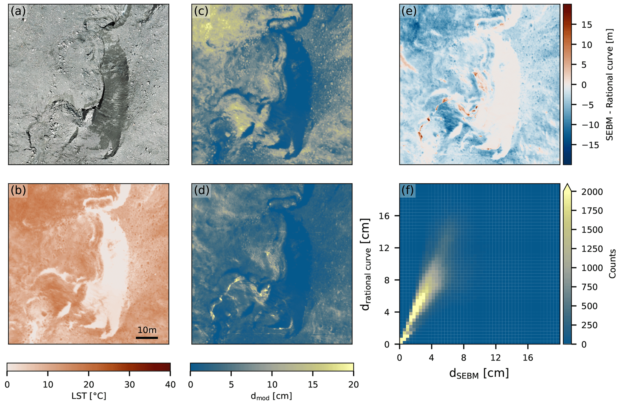
Figure 13 High-resolution subsection of the unpiloted aerial vehicle (UAV) imagery with debris cover, large boulders, and an ice cliff. The panels show (a) the RGB image, (b) the land surface temperature at 15:00 (UTC+1), (c) debris-thickness prediction using the rational curve approach, and (d) debris-thickness prediction by solving the surface energy balance model. The difference map (e) and 2D histogram (f) show how the model predictions compare spatially.

So far, the conversion of LST to debris thickness in high resolution has only been studied using ground-based oblique viewing angles (Herreid, 2021) using empirical equations. However, challenges in this approach include (1) the area covered by the field of view, (2) the variable path radiance, and (3) the viewing angle that controls the amount of radiation received by the sensor. The use of UAVs offers opportunities to overcome these issues but also faces challenges that we discuss here. These challenges stem from the specifics of image acquisition, limited battery lifetime, postprocessing requirements, and the conversion of the brightness temperature to LSTs.

All high-resolution studies, including ours, have so far used uncooled microbolometers, a sensor type that requires thermal equilibrium between the sensor device and the environment for accurate measurements (Budzier and Gerlach, 2015). As these conditions are difficult to achieve and maintain in high-mountain settings, the obtained thermal infrared images require calibration and correction. The ambient temperature difference between the ground and the flight elevation requires the sensor device to thermally adjust after takeoff, which thus introduces a measurement bias that varies with time (Fig. 2a). While this effect is primarily relevant for UAV applications, the maintenance of stable environmental conditions (e.g., changing wind speeds) cannot be guaranteed even for ground-based measurements, and temporal variance of the measurement bias should be considered. While the sensor device cools down after takeoff due to flight altitude, direct incident shortwave radiation may cause the device to heat up (Dugdale et al., 2019). The change in the measurement bias with time, the thermal drift, is partially balanced by the internal in-flight calibration of uncooled microbolometers (Mesas-Carrascosa et al., 2018), leading to recurring systematic jumps in the measured temperature (Fig. 2) that can be compensated for in a postprocessing step (see Sect. 3.2). Long flight times, slow flight speeds, and no direct shortwave radiation would thus minimize the effect of thermal drift but would likely not substitute for additional calibration.

The thermal correction during postprocessing in our case included (1) recovering the occurrence of flat field correction (FFC) events that were “lost” by the reduced sampling rate, (2) identifying and correcting the thermal drift, and (3) correcting the residual measurement bias using bare-ice surfaces. During all flight times, thermal drift corrected for by FFC events was rather large and resulted in changes by up to ∼ 8 K over 50 frames (Fig. 2a). With a frame rate of 1 s⁻¹, this means a thermal drift of up to 0.16 K s⁻¹. Assuming that the thermal drift is indeed linear with time, the in-flight FFC, or, as in our case, postprocessing identification of FFC, is relatively straightforward, due to the step change in LSTs across an FFC event. Figure 2a also shows the internal housing temperature and the temperature of the focal plane array, as recorded by the thermal sensor. The rapid decline, in the beginning, shows the thermal adjustment due to the vertical temperature gradient between the ground and flight elevation. While UAVs with larger battery capacity might offset this effect to some extent, our setup was limited at that point.

To convert the brightness temperature to LSTs, we accounted for the reflected portion of the incoming longwave radiation and surface-type emissivity but neglected the path radiance between the sensor and the ground. As the elevation of the UAV aboveground does not change significantly throughout the flight, the potential measurement bias of longwave radiation emitted by atmospheric water vapor content is minimized and assumed to be constant. Our “bulk” calibration approach using spline interpolation of measured ice surface temperatures compensates for the systematic temporal variability of the measurement bias (Fig. 2b) introduced by (1) thermal adjustment after takeoff, (2) fluctuations of atmospheric conditions by wind or incident direct shortwave radiation, or (3) longwave radiation emitted from atmospheric water vapor content or the surrounding terrain (Aubry-Wake et al., 2015; Aragon et al., 2020; Herreid, 2021).

Because of the need to calibrate all thermal images, the requirement of spatially well-distributed reference temperatures is the main drawback of the proposed method. In our case, bare-ice surfaces were present in the central part but not at the glacier's sides. Two image regions are found to be severely erroneous, an anomalously low-temperature patch on the eastern edge at 11:00 and a warm-temperature strip in the center that seems to follow the flight path of the UAV at 15:00 (Fig. 3b, d). We think the cold region at 11:00 could be due to a failed drift compensation, as the spline interpolation assumes a constant correction value before the first and after the last occurrence of bare ice in the thermal images. The warm-temperature strip could be related to an oblique viewing angle of the sensor during that flight, as the sensor alignment was done manually (Sobrino and Cuenca, 1999; Byerlay et al., 2020; FLIR, 2020).

So far, we have discussed the challenges and needs to derive glacier surface LSTs. Provided the measurements obtained in our experiment, we also observed differences in the resulting debris thickness that we derived from the SEBM and the rational curve approaches. The SEBM approach requires meteorological input data, assumptions on debris properties (in space and time), and substantial simplifications of SEB components. Because the conservation of energy represents a balance among all energy fluxes, it follows that any simplification in one component will have a quantitative effect on the others (Price, 1985). However, when comparing the diurnal variation of the energy flux components with measured quantities in a comparable setting regarding location, time, and debris thickness (Brock et al., 2010), we find good agreement in magnitude and distribution for net shortwave, net longwave, and change in heat storage and the conductive heat flux (Fig. 6). The possibility to estimate sub-daily surface energy balance components improves our understanding of ΔS. Repeated LST measurements might additionally increase understanding of the spatial variability of debris properties (e.g., thermal conductivity, debris density, or specific heat capacity) by quantifying the thermal inertia.

The accuracy of predicting debris thickness using a SEBM and empirically using a rational curve yielded comparable results with RMSEs of 6–8 cm depending on the time of the day. Both methods yield a terrain aspect bias. The SEBM approach compensates for the terrain effect to some degree, as the amount of incident shortwave radiation is a function of aspect, too. The terrain bias in the early flights using the rational curve approach is more pronounced, as it is only based on the LSTs. However, as this approach is less sensitive to uncertainties in LSTs, we recommend the rational curve approach to estimate debris thickness as long as enough debris-thickness measurements are available. Steep moraines of debris or hummocky-shaped debris-covered surfaces are likely to introduce bias via mixed-pixel effects, when predicting debris thickness using coarse-spatial-resolution LSTs from remote sensing data, especially in the case of empirically derived debris thicknesses. For example, the time of overpass of the Landsat satellite is typically between 10:00 to 11:00 locally, a time when debris cover is still heating up. Therefore, the effect of aspect on satellite-derived LST debris-thickness estimates should be studied in more detail.

6 Conclusions

In our experiment, we mapped supraglacial debris cover using high-resolution UAV-derived LST measurements at various times of the day and using two common approaches to create debris-thickness maps: a surface energy balance model approach and a simple extrapolation approach using a rational curve that relies on field measurements. We conclude the following:

1. Measuring the LSTs from a UAV using an uncooled microbolometer requires temperature calibration that varies with time. Here we determine an offset correction value for each thermal infrared frame by interpolating splines of spatially well-distributed bare-ice surfaces, assuming the ice to be at a melting point of 0 ^∘C. This bulk correction compensates for several sources of uncertainties but requires the presence of bare-ice surfaces.

2. Quantifying the surface energy balance components based on the UAV-derived LST measurements led to debris-thickness predictions with an RMSE of 6–8 cm, depending on the time of the day. Debris thicknesses were underestimated at all flight times. Measuring the diurnal variability of LSTs allowed us to extend the commonly used surface energy balance approach by quantifying the rate of change of heat storage.

3. The non-linearity of the relationship between LST and debris thickness increases with LST. Choosing the best empirical function for predicting debris thickness thus depends on the time of the day. Morning conditions yield a strong terrain aspect bias, which is better accounted for in the SEBM approach. When the LST reaches its diurnal maximum, here at 13:00 or 15:00, the non-linearity is most evident. Towards the evening the relationship between debris thickness and LST appears almost linear, and aspect plays a minor role.

4. Practical considerations for quantifying supraglacial debris cover using UAV-derived LSTs comprise LST calibration, choosing the model based on the time of the day, and debris-thickness measurements for evaluation. In our case, the ultra-lightweight UAV setup was suitable for remote high-mountain fieldwork but had a significant drawback due to the limited battery capacity, resulting in short flight times of 10 to 15 min and small spatial coverage. Consequently, the thermal adjustment of the device led to strong thermal drift and thus to many in-flight calibration events that had to be considered. Maximizing the flight time by using a larger UAV could offset this effect to some degree. The measurement bias varies with time, and spatially well-distributed reference temperatures should be used for calibration.