the Creative Commons Attribution 4.0 License.
the Creative Commons Attribution 4.0 License.
 | 15 Feb 2021
Sensitivity of ice sheet surface velocity and elevation to variations in basal friction and topography in the full Stokes and shallow-shelf approximation frameworks using adjoint equations
Nina Kirchner
Per Lötstedt
Predictions of future mass loss from ice sheets are afflicted with uncertainty, caused, among others, by insufficient understanding of spatiotemporally variable processes at the inaccessible base of ice sheets for which few direct observations exist and of which basal friction is a prime example. Here, we present a general numerical framework for studying the relationship between bed and surface properties of ice sheets and glaciers. Specifically, we use an inverse modeling approach and the associated time-dependent adjoint equations, derived in the framework of a full Stokes model and a shallow-shelf/shelfy-stream approximation model, respectively, to determine the sensitivity of grounded ice sheet surface velocities and elevation to time-dependent perturbations in basal friction and basal topography. Analytical and numerical examples are presented showing the importance of including the time-dependent kinematic free surface equation for the elevation and its adjoint, in particular for observations of the elevation. A closed form of the analytical solutions to the adjoint equations is given for a two-dimensional vertical ice in steady state under the shallow-shelf approximation. There is a delay in time between a seasonal perturbation at the ice base and the observation of the change in elevation. A perturbation at the base in the topography has a direct effect in space at the surface above the perturbation, and a perturbation in the friction is propagated directly to the surface in time.
- Article
(2503 KB) - Full-text XML
- BibTeX
- EndNote


Over the last decades, ice sheets and glaciers have experienced mass loss due to global warming, both in the polar regions and also outside of Greenland and Antarctica (Farinotti et al., 2015; Mouginot et al., 2019; Pörtner et al., 2019; Rignot et al., 2019). The most common benchmark date for which future ice sheet and glacier mass loss and associated global mean sea level rise is predicted is the year 2100 CE, but recently, even the year 2300 CE and beyond are considered (Pörtner et al., 2019; Steffen et al., 2018). Global mean sea level rise is predicted to continue well beyond 2100 CE in the warming scenarios typically referred to as RCPs (representative concentration pathways; see van Vuuren et al., 2011), but rates and ranges are afflicted with uncertainty, caused by, among others, insufficient understanding of spatiotemporally variable processes at the inaccessible base of ice sheets and glaciers (Pörtner et al., 2019; Ritz et al., 2015). These include the geothermal heat regime, subglacial and base-proximal englacial hydrology, and particularly the sliding of the ice sheet and glaciers across their base, for which only few direct observations exist (Fisher et al., 2015; Key and Siegfried, 2017; Maier et al., 2019; Pattyn and Morlighem, 2020).
In computational models of ice dynamics, the description of sliding processes, including their parametrization, plays a central role and can be treated in two fundamentally different ways, viz. using a so-called forward approach on the one hand or an inverse approach on the other hand. In a forward approach, an equation referred to as a sliding law is derived from a conceptual friction model and provides a boundary condition to the equations describing the dynamics of ice flow (in glaciology often referred to as the full Stokes (FS) model), which, once solved, render, e.g., ice velocities part of the solution. Studies of frictional models and resulting sliding laws for glacier and ice sheet flow emerged in the 1950s – see, e.g., Fowler (2011), Iken (1981), Lliboutry (1968), Nye (1969), Schoof (2005), and Weertman (1957) – have subsequently been implemented into numerical models of ice sheet and glacier behavior – e.g., in Brondex et al. (2017), Brondex et al. (2019), Gladstone et al. (2017), Tsai et al. (2015), Wilkens et al. (2015), and Yu et al. (2018) – and continue to be discussed (Zoet and Iverson, 2020), occasionally controversially (Minchew et al., 2019; Stearn and van der Veen, 2018).
Because few or no observational data are available to constrain the parameters in such sliding laws (Minchew et al., 2016; Sergienko and Hindmarsh, 2013), actual values of the former, and their variation over time (Jay-Allemand et al., 2011; Schoof, 2010; Sole et al., 2011; Vallot et al., 2017), often remain elusive. Yet, they can be obtained computationally by solving an inverse problem provided that observations of, e.g., ice velocities at the ice surface and elevation of the ice surface are available (Gillet-Chaulet et al., 2016; Isaac et al., 2015). Note that the same approach, here described for the case of the sliding law, can be used to determine other “inaccessibles”, such as optimal initial conditions for ice sheet modeling (Perego et al., 2014), the sensitivity of melt rates beneath ice shelves in response to ocean circulation (Heimbach and Losch, 2012), the geothermal heat flux at the ice base (Zhu et al., 2016), or to estimate basal topography beneath an ice sheet (Monnier and des Boscs, 2017; van Pelt et al., 2013). The latter is not only difficult to separate from the determination of the sliding properties (Kyrke-Smith et al., 2018; Thorsteinsson et al., 2003), but also has limitations related to the spatial resolution of surface data and/or measurement errors; see Gudmundsson (2003, 2008) and Gudmundsson and Raymond (2008).
Adopting an inverse approach, the strategy is to minimize an objective function describing the deviation of observed target quantities (such as the ice velocity) from their counterparts as predicted following a forward approach when a selected parameter in the forward model (such as the friction parameter in the sliding law) is varied. The gradient of the objective function is computed by solving the so-called adjoint equations to the forward equations, where the latter often are slightly simplified, such as by assuming a constant ice thickness or a constant viscosity (MacAyeal, 1993; Petra et al., 2012). However, when inferring friction parameter(s) in a sliding law using an inverse approach, recent work (Goldberg et al., 2015; Jay-Allemand et al., 2011) has shown that it is not sufficient to consider the time-independent (steady-state) adjoint to the momentum balance in the FS model. Rather, it is necessary to include the time-dependent advection equation for the ice surface elevation in the inversion. Likewise, but perhaps more intuitively understandable, the choice of the underlying glaciological model (FS model vs., e.g., shallow-shelf/stream approximation (SSA) model; see Sect. 2) has an impact on the values of the friction parameters obtained from the solution of the corresponding inverse problem (Gudmundsson, 2008; Schannwell et al., 2019). A related problem is to find the relation between perturbations of the friction parameters and the topography at the base and the resulting perturbations of the ice velocity and the elevation at the surface. The parameter sensitivity of the solutions is studied in Gudmundsson (2008) and Gudmundsson and Raymond (2008) by linearizing the governing equations. They show that basal perturbations of short wavelength are damped when they reach the surface, but the effect of long wavelengths can be observed at the top.
Here, we present an analysis of the sensitivity of the velocity field and the elevation of the surface of a dynamic, grounded ice sheet (modeled by both FS and SSA, briefly described in Sect. 2) to perturbations in the sliding parameters contained in Weertman's law (Weertman, 1957) and the topography at the ice base. The perturbations in a velocity component or the ice surface elevation at a certain location and time are determined by the solutions to the forward equations and the associated adjoint equations of a grounded ice sheet. A certain type of perturbation at the base may cause a very small perturbation at the top of the ice. Such a basal perturbation will be difficult to infer from surface observations in an inverse problem. High-frequency perturbations in space and time are examples when little is propagated to the surface. This is also the conclusion in Gudmundsson and Raymond (2008), derived from an analysis differing from the one presented here. The adjoint problem that is solved here to determine this sensitivity (Sect. 3) goes beyond similar earlier works by MacAyeal (1993) and Petra et al. (2012) because it includes the time-dependent advection equation for the kinematic free surface. The key concepts and steps introduced in Sect. 3 are supplemented by detailed derivations, collected in Appendix A. The same adjoint equations are applicable in the inverse problem to compute the gradient of the objective function and to quantify the uncertainty in the surface velocity and elevation due to uncertainties at the ice base. Examples of uncertainties are measurement errors in the basal topography and unknown variations in the parameters in the friction model. Analytical solutions in two dimensions of the stationary adjoint equations subjected to simplifying assumptions are presented, from which the dependence of the parameters, on, e.g., friction coefficients and bedrock topography, becomes obvious. The time-dependent adjoint equations are solved numerically, and the sensitivity to perturbations varying in time is investigated and illustrated.
The sensitivity of the surface velocity and elevation to perturbations in the friction and topography is quantified in extensive numerical computations in a companion paper (Cheng and Lötstedt, 2020). The adjoint equations derived and studied analytically in this paper are solved numerically for the FS and SSA models in Cheng and Lötstedt (2020) and compared to direct calculations of the surface perturbations with the forward equations. Discrete transfer functions are computed and analyzed as in Gudmundsson (2008) for the relation between surface perturbations and basal perturbations. While Gudmundsson's analysis is based on Fourier analysis, the analysis in Cheng and Lötstedt (2020) relies on analytical solutions of the SSA equations. The analysis in this paper and the numerical experiments in Cheng and Lötstedt (2020) confirm the conclusion in Gudmundsson (2008) that the perturbations with a long wavelength and low frequency will propagate to the surface while those of a short wavelength and high frequency are damped.
In this section, the equations emerging from adopting a forward approach to describing ice dynamics are presented, together with relevant boundary conditions, for the FS (4) and SSA model (9), respectively. These, and the notation and terminology introduced here, provide the framework in which the adjoint equations are discussed in Sect. 3.
The flow of large bodies of ice is described with the help of the conservation laws of mass, momentum, and energy (Greve and Blatter, 2009), which together pose a system of nonlinear partial differential equations (PDEs) commonly referred to as the FS equations in glaciological applications. In the FS equations, nonlinearity is introduced through the viscosity in Glen's flow law, a constitutive relation between strain rates and stresses (Glen, 1955). Continental sized ice masses (ice sheets and, if applicable, their floating extensions known as ice shelves) are shallow in the sense that their vertical extension V is orders of magnitudes smaller than their horizontal extension L, such that the aspect ratio is on the order 10−2 to 10−3. The aspect ratio is used to introduce simplifications to the FS equations, resulting, e.g., in the shallow-ice (SIA) (Hutter, 1983), shallow-shelf (Morland, 1987), and shelfy-stream (MacAyeal, 1989) approximations, parts of which can be coupled to FS using ISCAL (Ahlkrona et al., 2016), a method applicable to any FS framework and implemented in Elmer/Ice. They are all characterized by substantially reduced computational costs for numerical simulation, compared to using the FS model. A common simplification, also adopted in our analysis in the following, is the assumption of isothermal conditions, which implies that the balance of energy need not be considered.
The upper surface of the ice mass and also the ice–ocean interface constitute a moving boundary and satisfy an advection equation describing the evolution of its elevation and location (in response to mass gain, mass loss, or/and mass advection). For ice masses resting on bedrock or sediments, sliding needs to be parameterized at the interface. The interface between floating ice shelves and sea water in the ice shelf cavities is usually regarded as frictionless.
2.1 Full Stokes model
We adopt standard notation and denote vectors in bold italics and matrices in three-dimensional space in bold, and we denote derivatives with respect to the spatial coordinates and time by subscripts x, y, z, and t. The horizontal plane is spanned by the x and y coordinates, and z is the coordinate in the vertical direction (see Fig. 1a). Specifically, we denote by and u3 the velocity components of in the x,y, and z direction, where is the position vector and T denotes the transpose. Further, the elevation of the upper ice surface is denoted by , the elevation of the bedrock and the location of the base of the ice are b(x,y) and , and the ice thickness is . Upstream of the grounding line, γGL, zb=b, and downstream of γGL we have zb>b (see Fig. 1). In two dimensions, γGL consists of one point with x coordinate xGL.
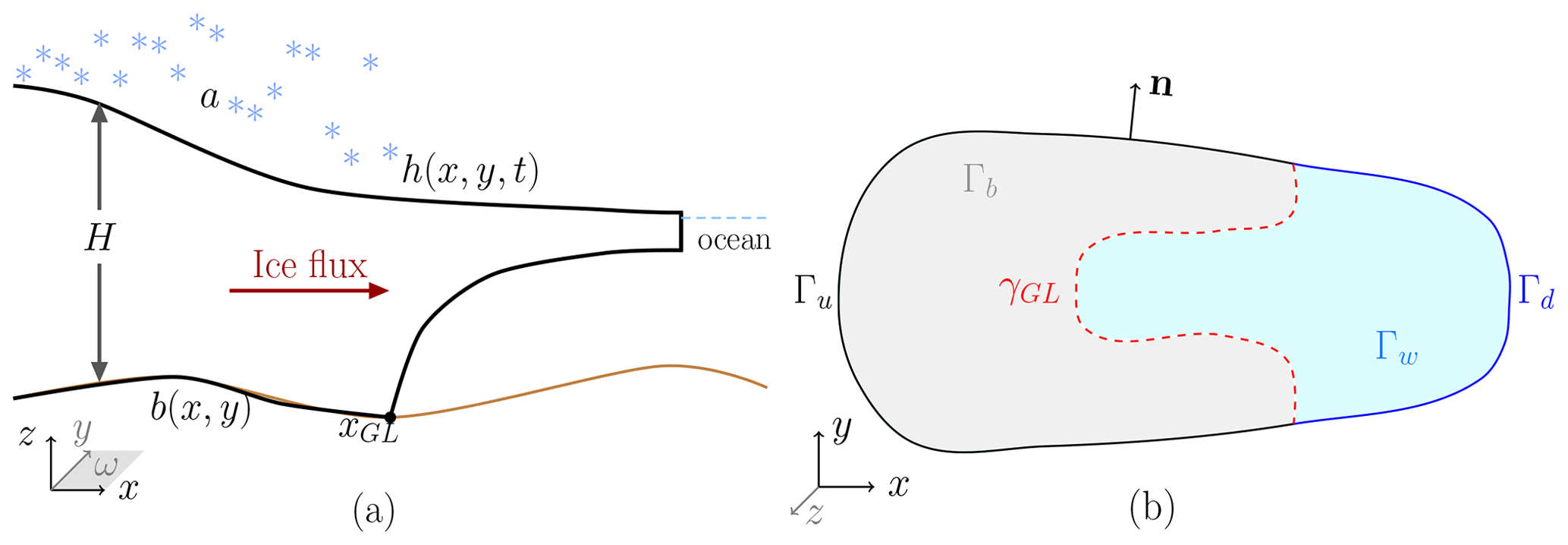
The boundary Γ enclosing the domain Ω occupied by the ice has different parts (see Fig. 1b). The lower boundaries of Ω are denoted by Γb (where the ice is grounded at bedrock) and Γw (where the ice has lifted from the bedrock and is floating on the ocean). These two regions are separated by the grounding line γGL, defined by (xGL(y),y) based on the assumption that ice flow is mainly along the x axis. The upper boundary is denoted by Γs (ice surface) at in Fig. 1a. The footprint (or projection) of Ω in the horizontal plane is denoted by ω and its boundary is γ.
The vertical lateral boundary (in the x–z plane, Fig. 1b) has an upstream part denoted by Γu in black and a downstream part denoted by Γd in blue, where . Obviously, if x∈Γu, then , or if x∈Γd, then , where . Letting n be the outward-pointing normal on Γ (or γ in two dimensions (x,y)), the nature of ice flow renders the conditions at Γu and at Γd. For a two-dimensional flow line geometry (Fig. 1a), this corresponds to and γd=L, where L is the horizontal length of the domain. In summary, the domains are defined as
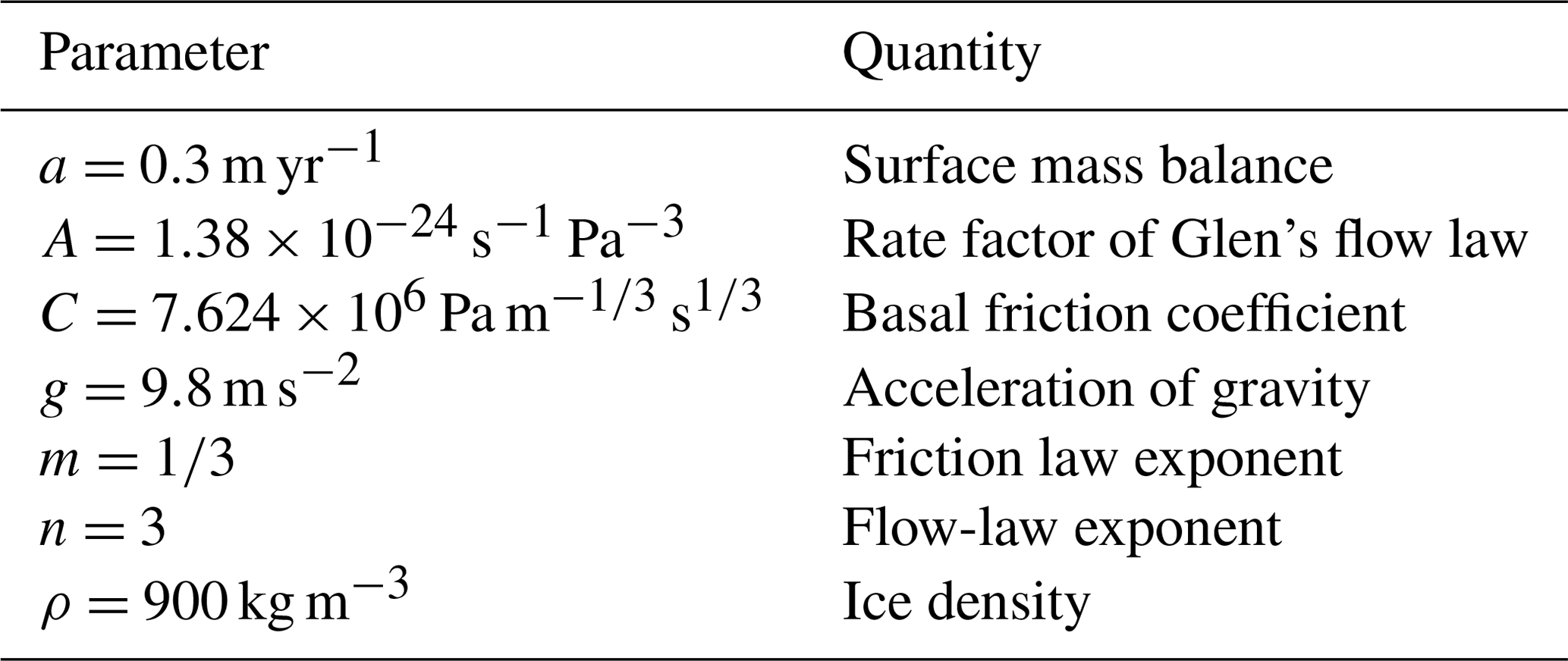
Before the forward FS equations for the evolution of the ice surface Γs and the ice velocity in Ω can be given, further notation needs to be introduced: ice density is denoted by ρ, accumulation and/or ablation rate on Γs by as, and gravitational acceleration by g. The values of these physical parameters are given in Table 1. On Γs, describes the spatial gradient of the ice surface (in two vertical dimensions ). The strain rate D and the viscosity η are given by
where trD2 is the trace of D2. The rate factor A in (2) depends on the temperature, and Glen's flow law determines n>0, here taken to be n=3. The stress tensor is
where p is the isotropic pressure and I is the identity matrix.
Turning to the ice base, the basal stress on Γb is related to the basal velocity using an empirical friction law , where a projection (Petra et al., 2012) on the tangential plane of Γb is denoted by , where the Kronecker outer product between two vectors a and c or two matrices A and C is defined by
The friction coefficient has a general form , where C(x,t) is independent of the velocity u and f(u) represents some linear or nonlinear function of u. For instance, with the norm introduces a Weertman-type friction law (Weertman, 1957) on ω with a Weertman friction coefficient and an exponent parameter m>0. Common choices of m are and 1.
With these prerequisites at hand, the forward FS equations and the advection equation for the ice sheet's elevation and velocity for incompressible ice flow are
where is the initial surface elevation and hγ(x,t) is a given height on the inflow boundary. In the floating ice, the equations and the boundary conditions are as above plus an equation for the free surface zb with zb≥b and a boundary condition on the wetted ice Γw:
where ab is the basal mass balance and pw is the water pressure at Γw. With the sea level at z=0 and the water density ρw, .
The solution at the grounding line satisfies a nonlinear complementarity problem. Let d be the distance between the ice base and the bedrock such that
On Γw, we have and and on Γb, we have and . The complementarity relation at the ice base Γb∪Γw can be summarized as
There are additional constraints on the solution. For example, the thickness of the ice is non-negative H≥0, there is a lower bound on the velocity in Weertmann's friction law, and there is an upper bound on the viscosity η. These conditions have to be handled in a numerical solution of the equations but are not discussed further here.
The boundary conditions for the velocity on Γu and Γd are of Dirichlet type such that
where uu and ud are known. These are general settings of the inflow and outflow boundaries which keep the formulation of the adjoint equations as simple as in Petra et al. (2014). Should Γu be at the ice divide, the horizontal velocity is set to . The ice velocity at the calving front is defined as ud to simplify the analysis. The vertical component of σn vanishes on Γu.
2.2 Shallow-shelf approximation
The three-dimensional FS problem (4) in Ω can be reduced to a two-dimensional, horizontal problem with by adopting the SSA, in which only is considered. This is because the basal shear stress is negligibly small at the base of the floating part of the ice mass, viz. the ice shelf, rendering the horizontal velocity components almost constant in the z direction (MacAyeal, 1989). The SSA is often also used in regions of fast flow over lubricated bedrock (MacAyeal, 1989).
The simplifications associated with adopting the SSA imply that the viscosity (see 2 for the FS model) is now given by
where , with . This η differs from (2) because B≠D due to the cryostatic approximation of p in the SSA. In (7), the Frobenius inner product between two matrices A and C is used, defined by . The vertically integrated stress tensor ς(u) (cf. 3 for the FS model) is given by
where H is the ice thickness (see Fig. 1). The friction law in the SSA model is defined as in the FS case. Note that basal velocity is replaced by the horizontal velocity. This is possible because vertical variations in the horizontal velocity are neglected in SSA. Then, Weertman's law is with a friction coefficient , just as in the FS model. In summary, the forward equations describing the evolution of the ice surface and ice velocities based on an SSA model (in which u is not divergence-free) read
Above, t is the tangential vector on such that and . The inflow and outflow normal velocities uu≤0 and ud>0 are specified on γu and γd. The lateral side of the ice γ is split into γg and γw with . There is friction in the tangential direction on γg which depends on the tangential velocity t⋅u with the friction coefficient Cγ and friction function fγ. There is no friction on the wet boundary γw. When the equations are solved for the grounded part, Ht=ht with a time-independent topography.
A flotation criterion determines the position of the grounding line (see, e.g., Seroussi et al. (2014)). The thickness H is compared to a flotation height Hf given by
If H>Hf then the ice is grounded and C>0 in (9). If H<Hf then it is floating with C=0. The grounding line is defined by H=Hf.
For ice sheets that develop an ice shelf, the latter is assumed to be at hydrostatic equilibrium. In such a case, a calving front boundary condition (Schoof, 2007; van der Veen, 1996) is applied at γd, in the form of the depth-integrated stress balance (ρw is the density of seawater):
2.2.1 The flow line model of SSA
In this section, the SSA equations are presented for the case of an idealized, two-dimensional vertical sheet in the x–z plane (see Fig. 1). The forward SSA equations are derived from (9) by letting H and u1 be independent of y and setting u2=0. Since there is no lateral force, Cγ=0. The position of the grounding line is denoted by xGL, and . Basal friction C is positive and constant where the ice sheet is grounded on bedrock, while C=0 at the floating ice shelf's lower boundary. To simplify notation, we let u=u1. The forward equations thus become
where uu is the speed of the ice flux at x=0 and ud is the speed at the calving front at x=L. If x=0 is at the ice divide, then uu=0. By the stress balance (10), the calving front satisfies
Assuming that u>0 and ux>0, the viscosity becomes , and the friction term with a Weertman law turns into Cf(u)u=Cum.
2.2.2 The two-dimensional forward steady-state solution
We now discuss the steady-state solutions to the system (11). Except for letting all time derivatives vanish, even the longitudinal stress can be ignored in the steady-state solution (see Schoof (2007)). With a sliding law in the form and the thickness given at xGL, (11) thus reduces to
The solution to the forward equation (12) is derived for the case when a and C are constant (for details, see D3 and D4 in Appendix D):
The solution is normalized with the ice thickness HGL=H(xGL) at the grounding line. Both xGL and HGL are assumed to be known in the formula. Similar equations to those in (12) are derived in Nye (1959) using the properties of large ice sheets. A formula for H(x) resembling (13) and involving H(0) is the solution of the equations. By including the longitudinal stress in the ice, an approximate, more complicated expression for H(x) is obtained in Weertman (1961).
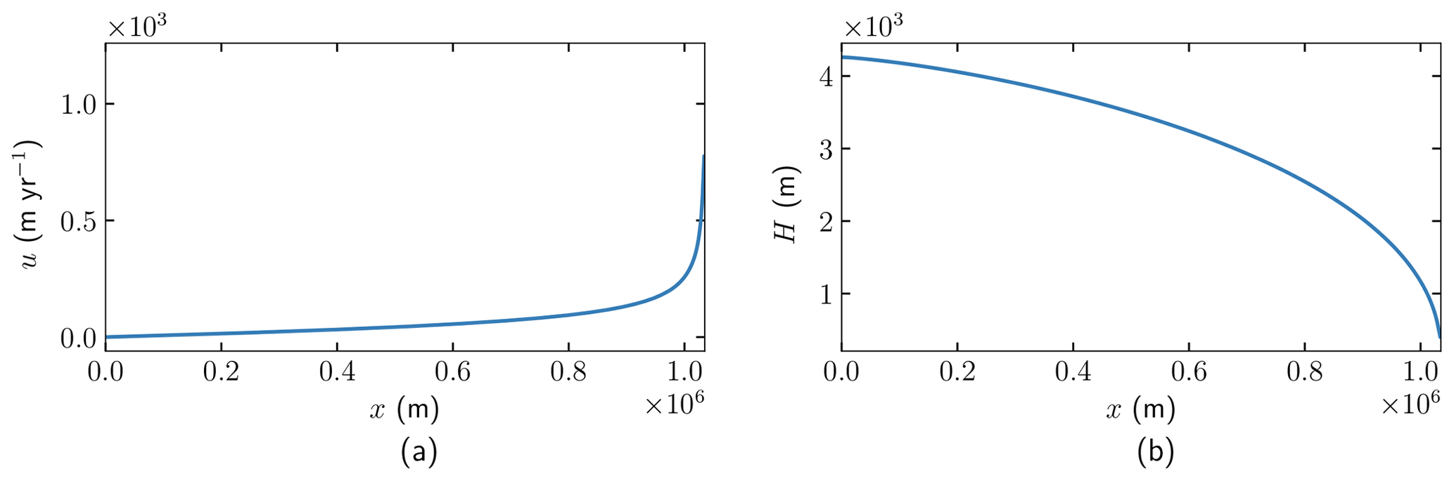
Figure 2 displays solutions from (13) obtained with data from the Marine Ice Sheet Model Intercomparison Project (MISMIP) (Pattyn et al., 2012) test case EXP 1 chosen in Cheng and Lötstedt (2020). The modeling parameters in (13) are given in Table 1. The ice sheet flows from x=0 to m on a single slope bed defined by and lifts from it at the grounding line position m. As x approaches xGL, H decreases to become HGL at xGL in Fig. 2b.
The larger the friction coefficient C and accumulation rate a are, the steeper the decrease in H is in (13). The numerator in u increases and the denominator decreases when x→xGL, resulting in a rapid increase in u. The MISMIP example is such that the SSA solution is close to the FS solution. Numerical experiments in Cheng and Lötstedt (2020) show that an accurate solution compared to the FS and SSA solutions is obtained with u and H in (13) solving (12).
Finally, it is noted that an alternative solution to (11) valid for the floating ice shelf, x>xGL, but under the restraining assumption of H(x) being linear in x, is found in Greve and Blatter (2009).
In this section, the adjoint equations are discussed, as emerging in a FS framework (Sect. 3.1) and in a SSA framework (Sect. 3.2), respectively. We derive the adjoint equations for the grounded part of the ice sheet. There the friction coefficient can be perturbed with δC≠0, and a perturbation δb of the topography has a direct influence on the flow of ice. The adjoint equations follow from the Lagrangian based on the forward equations after partial integration. Lengthy derivations have been moved to Appendix A. A numerical example based on the MISMIP (Pattyn et al., 2012) used also in Cheng and Lötstedt (2020) illustrates the findings presented.
On the ice surface Γs and over the time interval [0,T], we consider the functional ℱ:
We wish to determine its sensitivity to perturbations in both the friction coefficient C(x,t) at the base of the ice and the topography of the base itself b(x), which is a smooth function in x. We distinguish two cases: u and h satisfy either the FS equation (4) or the SSA equation (9). Given ℱ, the forward solution to (4) or (u,h) to (9), and the adjoint solution or (v,ψ) to the adjoint FS and adjoint SSA equations (both derived in the following and in Appendix A), we introduce a Lagrangian . The Lagrangian for the FS equations is
with the Lagrange multipliers and ψ corresponding to the forward equations for and h. The effect of perturbations δC and δb in C and b on ℱ is given by the perturbation δℒ, viz.
Examples of F(u,h) in (14) are , and in an inverse problem, in which the task is to find b and C such that they match observations uobs and hobs at the surface Γs (see also Gillet-Chaulet et al., 2016; Isaac et al., 2015; Morlighem et al., 2013; and Petra et al., 2012). Another example is with the Dirac delta δ at x* to measure the time-averaged horizontal velocity u1 at x* on the ice surface Γs with
where T is the duration of the observation at Γs. If the horizontal velocity is observed at then and
The sensitivity in ℱ and u1 in (17) or (18) to perturbations in C and b is then given by (16) with the forward and adjoint solutions.
The same forward and adjoint equations are solved both for the inverse problem and the sensitivity problem but with different forcing function F in (14). If we are interested in how u1 changes at the surface when b and C are changed at the base by given δb and δC, then F is as in (18). The forward and adjoint equations are then solved once. In the inverse problem with velocity observations, ℱ is the objective function in a minimization procedure and . The change δℱ in ℱ is of interest when C and b are changed during the solution procedure. In order to minimize ℱ, δC and δb are chosen such that δℱ<0 and ℱ decreases with C+δC and b+δb and u is closer to uobs. Precisely how δC and δb are chosen depends on the optimization algorithm. This procedure is repeated iteratively, and b and C are updated by b+δb and C+δC until δℱ→0 and ℱ has reached a minimum. The forward and adjoint equations have to be solved in each iteration in the inverse problem.
3.1 Adjoint equations based on the FS model
In this section, we introduce the adjoint equations and the perturbation of the Lagrangian function. The detailed derivations of (19) and (22) below are given in Appendix A, starting from the weak form of the FS equation (4) on Ω and by using integration by parts, and applying boundary conditions as in Martin and Monnier (2014) and Petra et al. (2012).
The definition of the Lagrangian ℒ for the FS equations is given in (15) and (A15) in Appendix A. To determine in (15), the following adjoint problem is solved:
where the derivatives of F with respect to u and h are
Note that (19) consists of equations for the adjoint elevation ψ, the adjoint velocity v, and the adjoint pressure q. The equations are the same as when the derivatives are computed in the inverse problem except for the terms depending on F, which is the misfit between the numerical solution and the observation in the inverse problem. Compared to the steady-state adjoint equation for the FS equations discussed in Petra et al. (2012), an advection equation is added in (19) for the Lagrange multiplier ψ(x,t) on Γs with a right-hand side depending on the observation function F and one term depending on ψ in the boundary condition on Γs. The adjoint elevation equation for ψ can be solved independently of the adjoint stress equation since it is independent of v. If h is observed and Fh≠0 and Fu=0, then the adjoint elevation equation must be solved together with the adjoint stress equation. Otherwise, the term ψh is ignored in the right-hand side of the boundary condition of the adjoint stress equation and the solution is v=0 with δℱ=0 in (22); see below.
The adjoint viscosity and adjoint stress are
cf. also Petra et al. (2012). For the rank four-tensor ℐ, ℐijkl=1 only when ; otherwise ℐijkl=0. The ⋆ operation in (20) between a rank four-tensor 𝒜 and a rank two-tensor (viz. a matrix) C is defined by . In general, Fb(Tu) in (19) is a linearization of the friction law f(Tu) in (4) with respect to the variable Tu. For instance, with a Weertman-type friction law, ,
The perturbation of the Lagrangian function with respect to a perturbation δC in the slip coefficient C(x,t) involves the tangential components of the forward and adjoint velocities, Tu and Tv at the ice base Γb, and is given by
For this formula to be accurate, δC has to be small. Otherwise, nonlinear effects may be of importance.
3.1.1 Time-dependent perturbations
Let us now investigate the effect of time-dependent perturbations in the friction parameter on modeled ice velocities and ice surface elevation. Suppose that the velocity component is observed at at the ice surface as in (18) and that , then
with and Fh=0. Above, we have introduced the simplifying notation that a variable with subscript * is a shorthand for it being evaluated at or, if it is time independent, at x*. Here we have chosen to consider the perturbation at a certain point in space and time , which is sufficient because other types of sensitivity over a certain period of time and space as in (17) are the linear combination of point-wise sensitivities.
The procedure to determine the sensitivity is as follows. First, the forward equation (4) is solved for u(x,t) and h(x,t) from t=0 to t=T. Then, the adjoint equation (19) is solved backward in time (from t=T to t=0) with as the corresponding final condition. Obviously, the solution for is and . Letting ei denote the unit vector with 1 in the ith component, the boundary condition in (19) becomes at . For , . Since ψ is small for (see Sect. 3.1.4), the dominant part of the solution is for some v0.
We start by investigating the response of ice velocities to perturbations in friction at the base: when the slip coefficient at the ice base is changed by δC, then the change in u1∗ at Γs is, according to (22), given by
This implies that the perturbation δu1∗ mainly depends on δC at time t* and that contributions from previous are small. If we observe the horizontal velocity, then it responds instantaneously in time to the change in basal friction.
Further, to investigate the response of the ice surface elevation, h* at Γs, to perturbations in basal friction, one considers
The solution of the adjoint equation (19) with at Γs for v(x,t) is non-zero since for .
In applied scenarios, friction at the base of an ice sheet is expected to exhibit seasonal variations. These can be expressed by , viz. a time-dependent perturbation added to a stationary time average C(x), with . If, for illustrational purposes, τ=1 (1 year, from January to December), then Northern Hemisphere cold and warm seasons can in a simplified manner be associated with (winter) and , (summer).
Assume further that f(Tu)Tu⋅Tv is approximately constant in time. This is the case if u varies slowly in time. Then ψ≈constant and v≈constant for . The change in ice surface elevation, δh, due to time-dependent variations in basal friction varies as
where the integral 𝒥 is
Obviously, from the properties of the cosine function, the friction perturbation δC is large at and vanishes at . Yet, (25) shows that at (during maximal friction in the winter) and at (during minimal friction in the summer), while when δC=0 at in the spring and the fall. The response in h by changing C is delayed in phase by or in time by years. This is in contrast to the observation of u1 in (24) where a perturbation in C is directly visible.
Particularly in an inverse problem where the phase shift between δC and δh in (25) is not accounted for, if h* is measured in the summer with , then the wrong conclusion would be drawn such that there is no change in C.
In another example, suppose that there is an interval with a step change of C with , where s(t)=1 in the time interval [t0,t1] and 0 otherwise. Then with 𝒥 in (26), δh* in (25) is
The effect of the basal perturbation successively increases in the elevation when and stays at a higher level for when δC has vanished.
3.1.2 Example with seasonal variation
To illustrate the phase delay in an oscillatory perturbation, a two-dimensional numerical example is shown in Fig. 3, where the timescale and friction coefficient are chosen as follows: τ=1 year, in m. We reuse the MISMIP (Pattyn et al., 2012) test case EXP 1 as in Sect. 2.2.2. The parameters of the setup are the same as in Fig. 2 and are given in Table 1. The variables u1 and h are observed at m. The steady-state solution of the forward equation with the GL located at m is perturbed by δu1 and δh when C is perturbed by δC as expressed in formulas and . After perturbation, the GL position will oscillate in time. The ice sheet is simulated by FS with Elmer/Ice (Gagliardini et al., 2013) for 10 years using the method implemented there for the position of the grounding line.
Figure 3 shows that the perturbations δu1 and δh in the grounded part of the ice sheet, specifically at and 1.02×10⁶ m for which individual panels are shown, oscillate regularly with a period of 1 year. The perturbations are small outside the interval . The initial condition at t=0 is the steady-state solution of the MISMIP problem and the FS solution with a variable C is essentially that steady-state solution plus a small oscillatory perturbation, as in Fig. 3.
The weight f(Tu)Tu⋅Tv0 in (24) is negative, and an increase in the friction, δC>0, leads to a decrease in the velocity, and δC<0 increases the velocity in all panels of Fig. 3. The velocities δu1 and the surface elevations δh are separated by a phase shift in time, , as predicted by (24) and (25).
The weight in (25) for δC0 in the integral over x changes sign when the observation point is passing from to 1.0×10⁶, explaining why the shift changes sign in the red dashed lines shown in the two lower panels of Fig. 3.
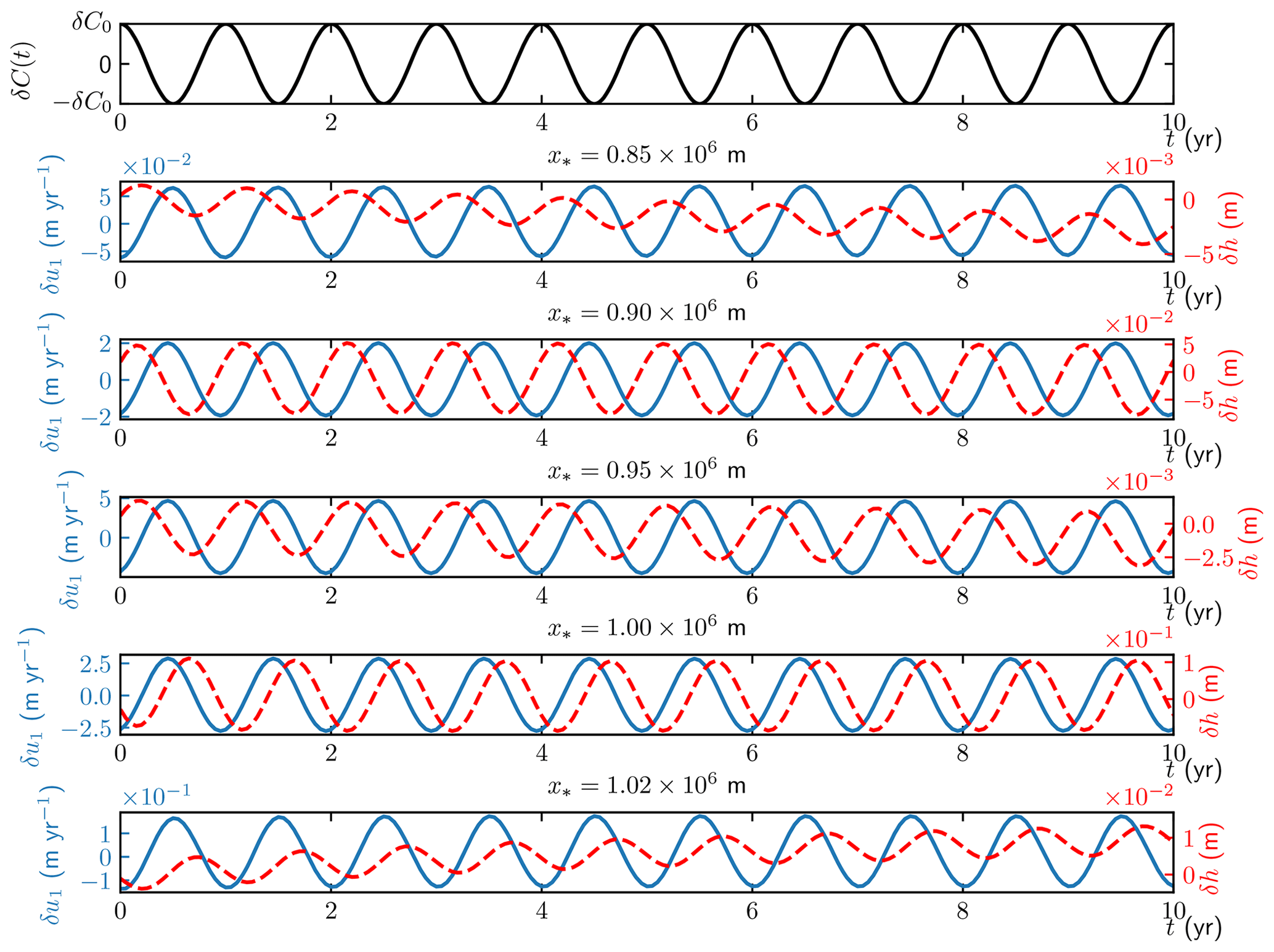
Figure 3Observations at m with FS in time of δu1 (solid blue) and δh (dashed red) with perturbation δC(t)=0.01Ccos (2πt) for m. Notice the different scales on the y axes.
3.1.3 The sensitivity problem and the inverse problem
From a theoretical point of view, it is interesting to note that there is a relation between the sensitivity problem where the effect of perturbed parameters in the forward model is estimated and the inverse problem used to infer “unobservable” parameters such as basal friction from observable data, e.g., ice velocity at the ice sheet surface. The same adjoint equation (19) are solved in both problems but with different driving functions defined by F(u,h) in (14).
Let be the steady-state solution to (19) when ui is observed at and . These are solutions to the sensitivity problem. We will show that the adjoint solution and the variation δℱ of the inverse problem can be expressed in . The perturbation δC is chosen such that δℱ<0 in each step in the iterative solution of the inverse problem. Then the objective function ℱ decreases stepwise toward the minimum.
It is shown in Appendix B that
is a solution of (19) with arbitrary weights when
When C is perturbed, the first variation of the functional in (22) is
In the inverse problem in Petra et al. (2012),
The weights in (27) for the inverse problem are . Let denote a weighted sum of the solutions of the sensitivity problem vi over the whole domain ω:
Then the effect of δC on ℱ in the inverse problem is by (28)
The same construction of the solution is possible when hobs is given. Then d=1, , and .
We have investigated the relation between the sensitivity problem and the inverse problem. By solving d sensitivity problems with to obtain their adjoint solutions and combine them with the weights wi from Fu in (29) for the inverse problem, the adjoint solution to the inverse problem is (30). This solution can then be inserted into (28) to evaluate the effect in ℱ of a change in C as in (31). In practice, if we are interested in solving the inverse problem and determine δℱ in (28) in order to iteratively compute the optimal solution with a gradient method, then we solve (19) directly with or to obtain without computing d vectors vi. Taking in (31) guarantees that δℱ<0.
3.1.4 Steady-state solution to the adjoint elevation equation in two dimensions
A further theoretical consideration shows that the solution ψ to the adjoint elevation equation need not be computed to estimate perturbations in the velocity for a two-dimensional vertical ice sheet at a steady state. We show with the analytical solution in the FS model that the influence of ψ is negligible. It is sufficient to solve the adjoint stress equation for v to estimate the perturbation in the velocity.
The adjoint steady-state equation in a two-dimensional vertical ice in (19) is
The velocity from the forward equation is , and the adjoint elevation ψ satisfies the right boundary condition ψ(L)=0.
The analytical solution ψ to (32) is derived in Appendix C. Let g(x)=u1z(x) if u1 is observed and let g(x)=1 if h is observed. Then the adjoint solution is
So, this solution has a jump at x*.
With a small in (33), an approximate solution is . If u1 is observed and , then ψ(x)≈0 in (33) and ψh≈0 in (19). This is the case in the SSA of the FS model where u1z(x)=0 and in the SIA of the FS equations where (Greve and Blatter, 2009; Hutter, 1983). When these approximations are accurate then u1z will be small. Consequently, when u1 is observed, the effect on v in the adjoint stress equation of the solution ψ of the adjoint advection equation in (19) is small. Solving only the adjoint stress equation for v as in Gillet-Chaulet et al. (2016), Isaac et al. (2015), and Petra et al. (2012) yields an adequate answer. Numerical solution in Cheng and Lötstedt (2020) of the adjoint FS equation (19) in two dimensions confirms that when u1 is observed then ψ(x) is negligible. The situation is different when h is observed and in (33).
3.2 Adjoint equations based on SSA
Starting from (9), a Lagrangian ℒ of the SSA equations is defined, using the technique described and applied to the FS equations in Petra et al. (2012). The SSA Lagrangian in (A4) in Appendix A is similar to the FS Lagrangian in (15). By partial integration in ℒ and evaluation at the forward solution (u,h), the adjoint SSA equations are obtained. Then, the effect of perturbed data at the ice base manifests itself at the ice surface as a perturbation δℒ; for details, see Appendix A.
The adjoint SSA equations read
where the adjoint viscosity and adjoint stress are (cf. 20 for the case of FS)
From (34) it is seen that the adjoint SSA equations have the same structure as the adjoint FS equation (19). There is one stress equation for the adjoint velocity v and one equation for the Lagrange multiplier ψ corresponding to the surface elevation equation in (9). However, the advection equation for ψ in (34) depends on v, implying a fully coupled system for v and ψ. Equations (34) are solved backward in time with a final condition on ψ at t=T. As in (9), there is no time derivative in the stress equation. With a Weertman friction law, viz. and (cf. also Appendix A1),
If the friction coefficient C at the ice base (both where it is grounded on bedrock (C>0) and floating (C=0)) is changed by δC, if the bottom topography is changed by δb, and if the lateral friction coefficient Cγ is changed by δCγ, then it follows from Appendix A2 that the Lagrangian ℒ is changed by (note that the weight in front of δC in Eq. 36 is actually the same as in Eq. 22)
The same perturbations in and δCγ could be allowed for the FS equations in (22), but because the FS equations are more complicated than the SSA equations, the complexity of the derivation in the appendix and the expression for δℒ would increase considerably, which is why we refrain from considering them here.
Suppose that only h is observed with Fh≠0 and Fu=0 in (34). Then the adjoint elevation equation must be solved for ψ≠0 to have a v≠0 in the adjoint stress equation and a perturbation in the Lagrangian in (36). The same result follows from the adjoint FS equations. If Fh≠0 and Fu=0 in (19), then ψ≠0. Consequently, v≠0 and a perturbation δC will cause a perturbation δℒ in (22). The conclusion that the adjoint elevation equation must be solved if the surface elevation is observed is independent of the two ice models.
In a broader context, it is worth emphasizing that the adjoint equation derived in MacAyeal (1993) is identical to the stress equation in (34), if H is constant, Fω=0 (e.g., m=1), and .
3.2.1 The two-dimensional adjoint solution
The adjoint SSA equations in two vertical dimensions are derived from (34) in the same manner as (11), by letting ψ and v1 be independent of y and setting v2=0 and Cγ=0. To simplify the notation, we also let v=v1. The adjoint equations for v and ψ follow either from simplifying (34) or from the Lagrangian and (11) and read as follows:
Note that the viscosity above is multiplied by a factor , n>0, which represents an extension of the adjoint SSA in MacAyeal (1993), where n=1 implicitly. The effect on the Lagrangian of perturbations δb and δC is obtained from (36):
The weights or sensitivity functions wb and wC multiplying δb and δC in the integral are defined by
The steady-state solutions to the system (37) can be analyzed as in the forward equations in Sect. 2.2.2 after simplifications. The viscosity terms in (37) are often small and can hence be neglected, and we assume that the basal topography is characterized by a small spatial gradient bx. The advantage resulting from these simplifications is that both the forward and adjoint equations can be solved analytically on a reduced computational domain where . The analytical approximations are less accurate close to the ice divide where some of the above assumptions are not valid. The adjoint equation (37) reduce to
3.2.2 The two-dimensional adjoint steady-state solution with velocity observation
In this section, the analytical solution to the adjoint equation (40) is discussed. The derivation of the solution is detailed in Appendix E to Appendix F. It is here sufficient to recall that the solution given below is derived under the assumptions that bx≪Hx, and that a and C are constants.
For observations of u at x*,
and the adjoint solutions are
where ψ(x) and v(x) have discontinuities at the observation point x*. The perturbation of the Lagrangian (38) is with the Heaviside step function ℋ(x) and the Dirac delta δ(x) (cf. Appendix F):
or, after scaling with u*,
The relation in (43) between the relative perturbations , and can also be interpreted as a way to quantify the uncertainty in u. The uncertainty may be due to measurement errors in the topography b. For example, it is known that the true surface is in an interval around b where, e.g., δb=1 m or δb has a normal distribution with zero mean and some variance. Such an uncertainty δb in b or similarly an uncertainty δC in C is propagated to an uncertainty δu* in u at x* by (43); see Smith (2014). As an example, suppose that a 5 % error in the surface velocity is acceptable, then the tolerable error in the topography could be 20–30 m with a 1000 m thick ice.
The perturbations δu1i at discrete points due to perturbations δCj at discrete points are connected by a transfer matrix WC in Cheng and Lötstedt (2020). The relation between δu1i and δCj is for all i and j such that
The elements WCij of the transfer matrix correspond to quadrature coefficients in the discretization of the first integral in (42) with δb=0. The properties of WC are examined numerically in Cheng and Lötstedt (2020). We conclude that certain perturbations of C (not only highly oscillatory) are difficult to observe in u1 at the surface. The same analysis is performed for the other combinations of δb,δC and δu1,δh.
Finally, let us comment on other approaches to investigate the sensitivity of surface data to changes in b and C, e.g., using three linear models as in Gudmundsson (2008) and along a flow line at a steady state in Gudmundsson and Raymond (2008) with a linearized FS model with n=1 and m=1. In these papers, transfer functions for the perturbations from base to surface corresponding to our formulas (42) and (43) are derived by Fourier and Laplace analysis. The perturbations with long wavelength λ and small wave number k are propagated to the surface, but short wavelengths are effectively damped in Gudmundsson (2008). The transfer functions are utilized in Gudmundsson and Raymond (2008) to estimate how well basal data can be retrieved from surface data. Retrieval of basal slipperiness C is possible for perturbations δC of long wavelength and if the error in the basal topography δb is small. Short wavelength perturbations δb can be determined from surface data. The same conclusions as in Gudmundsson (2008) and Gudmundsson and Raymond (2008) can be drawn from our explicit expressions for the dependence of δu* and δh* on δC and δb. For example, it follows from (45) that only δC with a long wavelength is visible at the surface and that δb also with a short wavelength affects δu* in (43). If δb is small or zero in (43), then it is easier to determine the δC that causes a certain δu*.
The analytical adjoint solutions ψ(x) and v(x) in (41) of the MISMIP case in Fig. 2 with parameters in Table 1 at different x* positions are shown in Figs. 4a and 5a.

Figure 4The analytical solutions of ψ in (40) of the observations of (a) u and (b) h at different locations , and 0.9×10⁶ m.
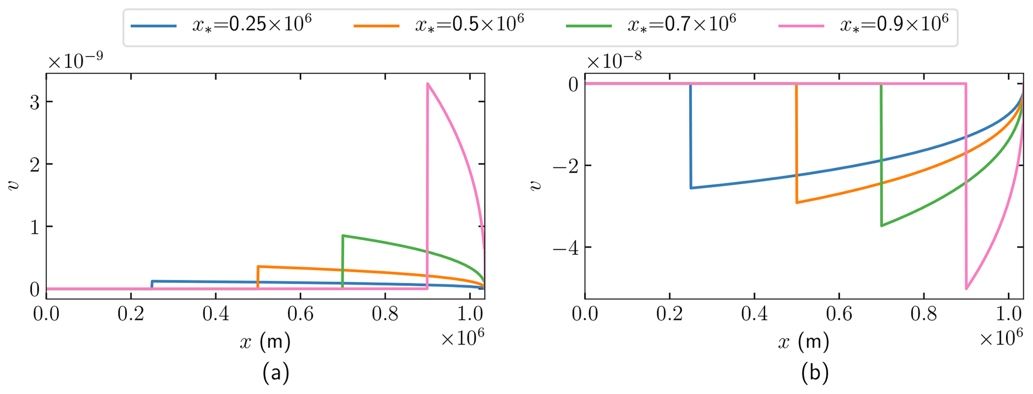
Figure 5The analytical solutions of v in (40) of the observations of (a) u and (b) h at different locations , and 0.9×10⁶ m.
The weights wb and wC in (42) multiplying δb and δC, defined in the same manner as in (38) and (39), are shown in Figs. 6a and 7a with the solutions ψ and v in Figs. 4a and 5a. The Dirac term is plotted as a vertical line at x* in Fig. 7a.
All perturbations in C between x* and xGL will result in a perturbation of the opposite sign in u* at the surface because wC<0 in in Fig. 6a and (42). The same conclusion holds true for perturbations in b because wb<0 in in Fig. 7a, but an additional contribution is added from δb at x* by the Dirac delta in wb. A perturbation is less visible in u the farther away from xGL the observation point is since the amplitude of both wC and wb decays when x* decreases.
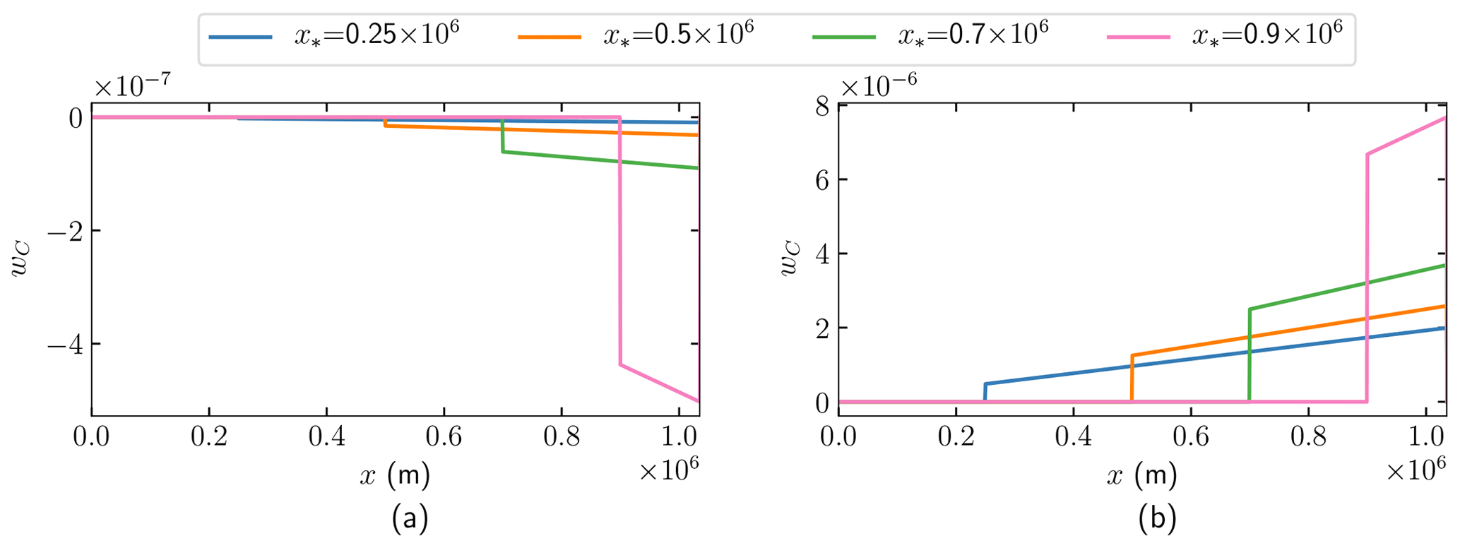
Figure 6The analytical solution of the weights on δC in (38) for (a) u and (b) h observed at , and 0.9×10⁶ m.
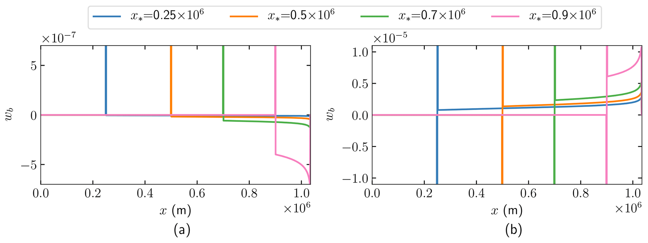
Figure 7The analytical solution of weights on δb in (38) for (a) u and (b) h observed at , and 0.9×10⁶ m.
The following conclusions can be drawn from (42) and (43) and Figs. 6 and 7.
- i
The closer perturbations in basal friction are located to the grounding line, the larger perturbations of velocity will be observed at the surface. This is because the weight in front of δC increases when , see Fig. 6, which in turn is an effect of the increasing velocity u* and the decreasing thickness H*, as the grounding line is approached (see Fig. 2). Or, compactly expressed, δC with support in will cause larger perturbations at the surface the closer x* is to xGL and the closer δC(x) is to xGL. The same conclusion is drawn in Cheng and Lötstedt (2020) with numerically computed SSA adjoint solutions.
- ii
Variations in the observed velocity δu* at the surface at observation point x* will include contributions from changes in the frictional parameter, δC, between x* and the grounding line xGL, as well as from changes in basal topography, δb, but it is impossible to disentangle their individual contributions to δu*.
- iii
When the variation in ice thickness is small compared to the overall ice thickness, Hx≪H, a small perturbation in basal topography δb is directly visible in the surface velocity. This is because in such a case, , and the main effect on u* from the perturbation δb is localized at each x* (see Eq. 42).
- iv
For an unperturbed basal topography, two different perturbations of the friction coefficient will result in the same perturbation of the velocity. In other words, the perturbation δC cannot be uniquely determined by one observation of δu. This follows if we let the perturbation of the friction coefficient be a constant δC0≠0 in and evaluate the integral in (42) to obtain
The same δu* is observed with a constant perturbation in with the amplitude .
- v
A rapidly varying friction coefficient at the base of the ice sheet will be difficult to identify by observing the velocity at the ice surface. In contrast, a smoothly varying friction coefficient at the base will be easily observable at the ice sheet surface. This is seen as follows: Perturb C by in (42) for some wave number k, which determines the smoothness of the friction at the bedrock and amplitude ϵ, and let δb=0 and m=1. The wavelength of the perturbation is . When k is small then the wavelength is long and the variation of C+δC is smooth. When k is large then the friction coefficient varies rapidly in x with a short λ. The perturbation in the velocity is
For a thin ice with a small H*, a perturbation in C is easier to observe at the surface than for a thick ice. When k grows at the ice base, the amplitude of the perturbation at the ice surface decays as . Thus, the effect of high wave number perturbations of C will be difficult to observe at the top of the ice, but smooth perturbations at the base will propagate to the surface. If k is large and the surface velocity is of interest in a numerical simulation, then there is no reason to use a fine mesh at the base to resolve the fast variation in C because it will not be visible at the top of the ice. How the damping depends on λ in the FS equations is computed in Cheng and Lötstedt (2020).
- vi
A perturbation in the topography with long wavelength is easier to detect at the surface than a perturbation with short wavelength. If δC=0 and b is perturbed by , then any perturbation at x* is propagated to the surface by , which is the first term on the right-hand side of (42). The effect is larger if the ice is thin and moving fast. The integral term will behave in the same way as in (45), with mainly perturbations with small wave numbers and long wavelengths visible at the surface.
3.2.3 The two-dimensional adjoint steady-state solution with elevation observation
In the case when h is observed at x* and Fu=0 and , the expressions for ψ and v satisfying (40) are
The corresponding formulas when u is observed are found in (41). There is a discontinuity at the observation point x* in v(x) illustrated in Fig. 5b, but ψ(x) is continuous in the solution of (40) and in Fig. 4b.
The second derivative term is neglected in the simplified Eq. (40) but is of importance at x*. A correction of ψ at x* in (46) is therefore introduced to satisfy . With , the correction is . The solution ψ is updated at each x* in Fig. 4b, with as a vertical line representing the negative Dirac delta.
The perturbation in h is as in (42) with ψ and v in (46) and the additional term :
where represents the x-derivative of uδb evaluated at x*. When δb=0 then δu* in (43) and in (47) satisfy as in the integrated form of the advection equation in (12) and in (D1) in the Appendix.
As in (42), (47) is rewritten with the weights wb and wC in (39):
These weights are shown in Figs. 6b and 7b. The negative derivative of the Dirac delta is depicted in Fig. 7b as a vertical line in the negative direction immediately followed by one in the positive direction.
The contribution from the integrals in (43) and (47) is identical except for the sign (compare wC in Fig. 6a and b and wb in Fig. 7a and b). The first term in (43) depends on , and the first term in (47) depends on the derivative of . The derivative of uδb at x* directly affects the perturbation of h at x*. A perturbation of b at the base is directly visible locally in u at the surface, while the effect of δC is non-local in the integral in (47). Because of the similarities between (43) and (47) and the left and right columns of Figs. 6 and 7, the conclusions (i), (ii), (iv), (v), and (vi) in Sect. 3.2.2 from (42) and (43) for δu* are valid also for δh* in (47).
3.2.4 The two-dimensional time-dependent adjoint solution
Finally, the time-dependent adjoint equation (37) is investigated. Equation (37) is solved numerically for the same MISMIP test case as Fig. 2 in Sect. 2.2.2 with the parameters in Table 1. As in Sect. 3.1.2, the friction coefficient C has a seasonal variation (period τ 1 year, where the beginning of the year is associated with winter) in the forward equation (11):
Apparently, C has its highest value at , i.e., the winter, and its lowest value at , i.e., the summer, as in Fig. 3. The amplitude of the variation in C is set to κ=0.5, and the forward equation (11) is solved for 11 years. The GL is determined by the conditions in Sect. 2.2 and will move in time because of the variation in C. The topography b is kept constant in time. Observations of u and h are made at m for 0.1 year in the four seasons starting from the summer of the 10th year, e.g., in the summer , the fall , the winter , and the spring . The forward equation (11) is solved numerically from t=0 with the steady-state solution as initial data to the observation points , and the adjoint equation (37) is solved from backward in time to t=0. According to a convergence test, the time step is chosen to be 0.01 year and the spatial resolution is 103 m. A visual inspection of the computed solutions after halving the step sizes indicates that a sufficiently converged numerical solution has been reached.
Figure 8 shows the results for the adjoint weights wC(x,t) and wb(x,t) multiplying the perturbations δC and δb, as defined in (38), for the observations of u and h at m in all four seasons, where each column represents one season. The friction coefficient C follows the seasonal variation in (49). Each row is one of the combinations of the weights wC and wb for the observations of u and h. The time axis (or ordinate) in the figure follows the time direction in the forward problem (11). Most of the weights in space and time are negligible, implying that perturbations in those domains are not visible at . Only δC and δb in a narrow interval around x* for t in have an influence on δu* and δh*. Therefore, we take a snapshot of the x axis (or abscissa) with the width of 105 m in space around x* in Fig. 8. The weights oscillate in time because of the seasonal variation in the basal conditions in (49). A perturbation at the base is propagated to the x* position on the surface but with a possible delay in time. The earlier a perturbation in C or b takes place in the interval , the smaller the effect of it is at t*. After 5 years a perturbation can hardly be detected at the surface.
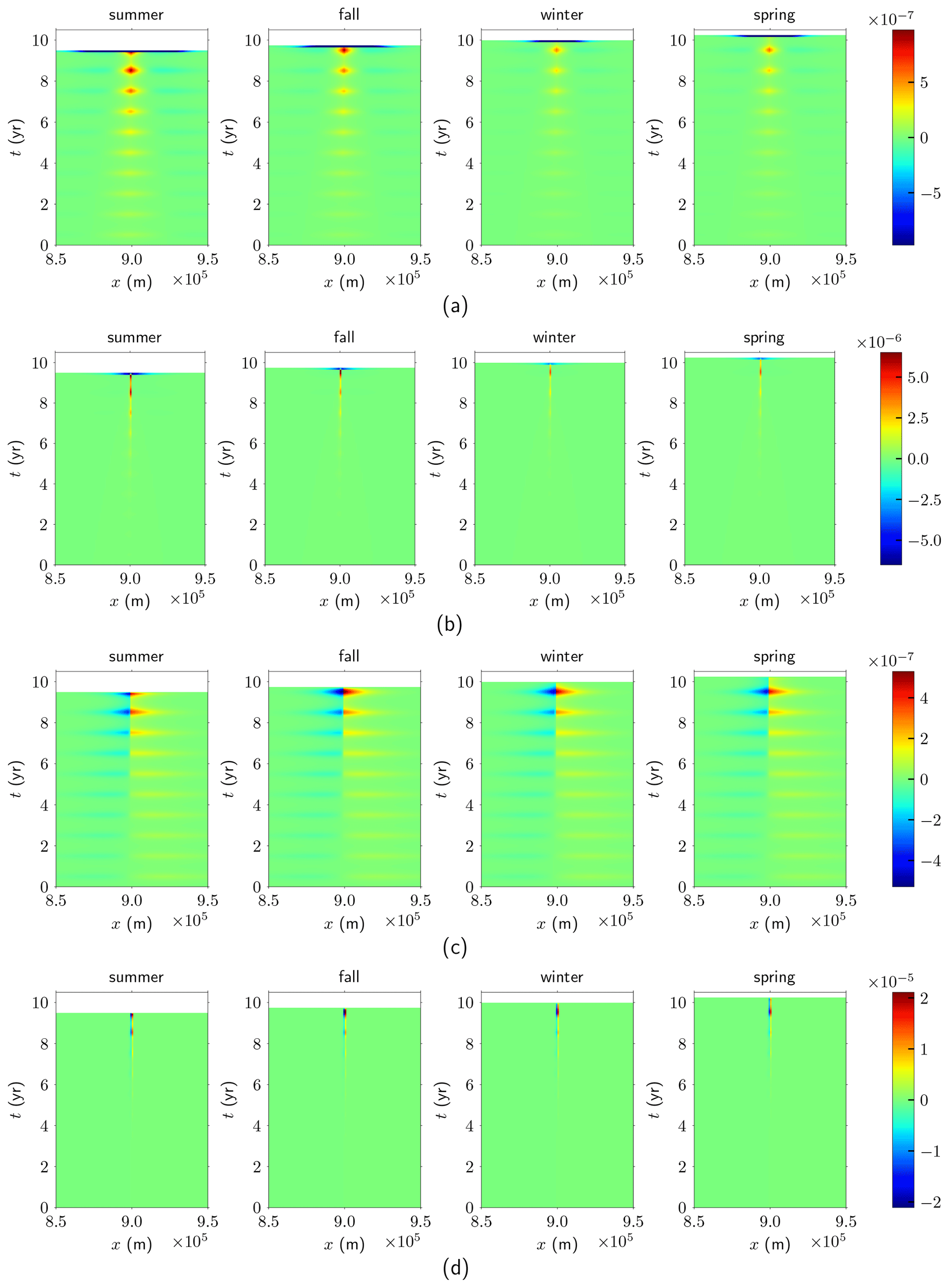
Figure 8The adjoint weights for the observations at m of the four seasons. (a) wC for the observation of u. (b) wb for the observation of u. (c) wC for the observation of h. (d) wb for the observation of h.
The temporal variations of the adjoint weights at x* in Fig. 8 are shown in Fig. 9 for the four seasons with four different colors. As expected, the weights vanish when . In Fig. 9a and b, the perturbations δC* and δb* have a direct effect on δu* at t*, where both and are negative. The same direct effect of δC is found for δu1∗ solving the FS equation (24) in Sect. 3.1.1. A change in δC* at the base is observed immediately as a change in u at the surface. The effect of δC on δu* for is weak in Fig. 9a; i.e., the memory of old perturbations is short. The largest effect of δC on δu* and δh* appears with t* in the summer when C is small in (49) (the blue lines in Fig. 9a and b).
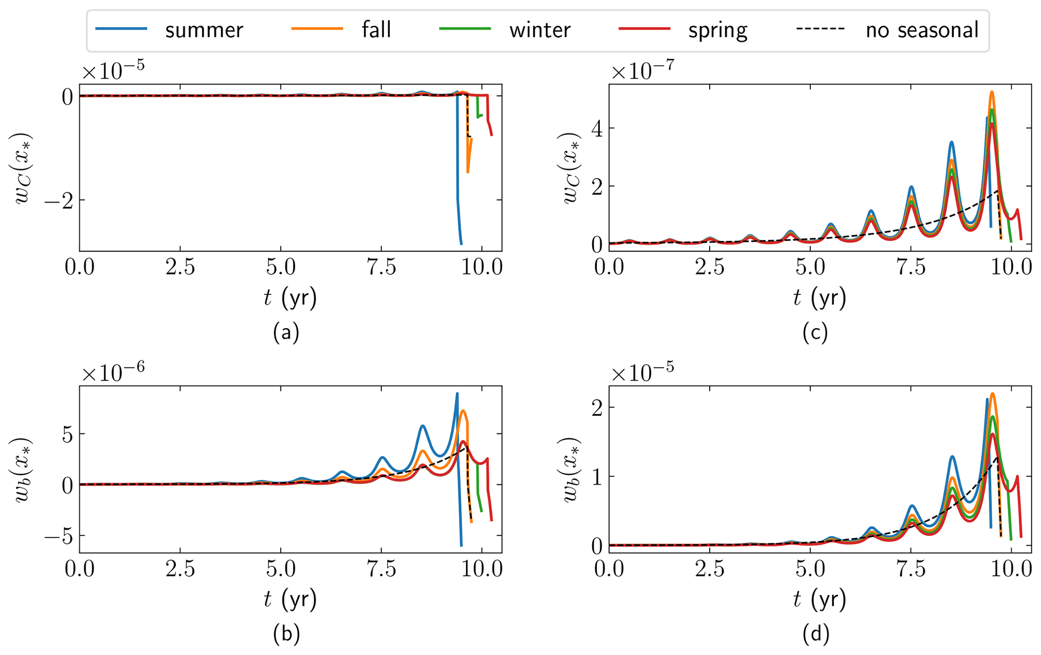
Figure 9The adjoint weights at x* in the four seasons of the 10th year with seasonally varying friction coefficient. The black dashed line is a reference solution without seasonal variations which is observed at . (a) wC for the observation of u. (b) wb for the observation of u. (c) wC for the observation of h. (d) wb for the observation of h.
However, when h is observed, the effects of δC* and δb* are not visible directly because and in Fig. 9c and d. An intuitive explanation is that there is an immediate effect on the velocity, but there is a delay in h since it is integrated in time from the velocity field. Additionally, the effects of δC and δb are difficult to separate, since the weight has a shape similar to . The largest effect on δh* is from δC in the summer due to the peaks in wC in Fig. 9c. For the same δC, the largest δh* is observed in the fall (orange), and then the second largest δh* is in the winter (green), followed by the spring observation (red). If δh* is observed in the fall and the time dependency is ignored, then the wrong conclusion is drawn that δC in the fall has the strongest effect (but it is the summer perturbation). There is a delay in time between the perturbation and the observation of the effect in the surface elevation. The same shift in time is what we found in Sect. 3.1.1, (25), and Fig. 3 for the FS equations.
A reference adjoint solution at x* observed during the fall season () with time-independent C and b, κ=0 in (49), as parameters in the forward equations is shown in black dashed lines in all the four panels of Fig. 9. The weight wb at x* for a constant b is well approximated by in time with τ=1.4 years for some wb∗ for the observation of both u and h in Fig. 9b and d. For the weight wC, the same exponential function holds with weight wC*, but the time constant τ=1.8 years for the observation of h* in Fig. 9c and τ=2.2 years for the u* case.
Suppose that the temporal perturbation is oscillatory with frequency f and located in space at x* with
A low-frequency f with f≪1 corresponds to decennial or centennial variations and a high-frequency f with f≫1 corresponds to diurnal or weekly variations. Then the perturbation in h at is
cf. (45). If the frequency is high, f≫1, then and high-frequency perturbations are damped efficiently. At certain times of observation t* when , the damping is even stronger with . If the frequency is low, f≪1, then and the change in h* is insensitive to the frequency. The same conclusions hold true for δb where decennial perturbations seem more realistic.
The adjoint equations are derived in the FS and the SSA frameworks including time and the surface elevation equation. Time-dependent perturbations δC and δb in basal friction coefficient C and basal topography b are introduced, and their effect on observations of the velocity u and the surface elevation h at the top surface of the grounded ice is studied. With the solution of the adjoint equations, we can determine the perturbation at a given point in space and time on the surface due to all basal perturbations. By solving the forward equations twice with C and C+δC or b and b+δb, we can compute the perturbation in all points in space and time on the surface, e.g., in the first velocity component, for a given δC or δb.
The perturbations in the observations are determined numerically in Cheng and Lötstedt (2020) either using the adjoint equations and their solutions in Sect. 3 or by solving the forward equations with unperturbed and perturbed parameters to obtain δu* and δh*. The numerical solutions are compared to each other and to analytical solutions for SSA. The agreement is good in the comparisons.
In Sect. 3.1.3, a relation is established between the inverse problem (aiming to infer parameters from data) and the sensitivity problem (aiming to quantify the effect of variations in parameters): the same adjoint equations are solved. However, the forcing functions differ and are specific to the inverse problem and the sensitivity problem, respectively. Common to both problems is that the adjoint equations tell how perturbations in the parameters at the ice base are propagated to perturbations in the velocity and the elevation of the surface.
For steady-state problems, and in an FS setting where u is observed, we find (cf. Sect. 3.1.4) that the contribution of the solution of the adjoint elevation equation (32) is small and that it therefore suffices to solve only the adjoint stress equations – see, e.g., Gillet-Chaulet et al. (2016), Isaac et al. (2015), and Petra et al. (2012) – in order to be able to draw conclusions regarding perturbations of u. For steady-state problems in a two-dimensional SSA setting for a vertical ice, (43), (47), and Figs. 6 and 7 show that the sensitivity of the velocity and elevation increases (because the velocity increases and the ice thickness decreases) as the observation point x* approaches the grounding line.
In this setting, a non-local effect of a perturbation in C has been observed, in the sense that δC(x) affects both u(x*) and h(x*) even if , but a perturbation δb in b has a strong local effect concentrated at x*. Nevertheless, the shapes of the two sensitivity functions (or weights) for δb and δC are very similar except for the neighborhood of x*, which makes it difficult to separate their respective contribution in an observation. Different combinations of the perturbations in the basal friction and bedrock elevation can produce the same effect on the velocity and surface elevation changes at one observation point.
In the inverse problems based on time-dependent simulations of FS and SSA, it is necessary to include the adjoint elevation equation. If the perturbations in the basal conditions are time dependent and h is observed (see Figs. 3, 9c, and d), then time cannot be ignored in the inversion. If time dependence is ignored, wrong conclusions concerning the conditions at the ice base may be drawn from observations of h, in both the FS and the SSA model. In the time-dependent solution of SSA, a perturbation of the basal condition at x* has the strongest impact at x* on the surface, possibly with a time delay. Such a time delay occurs when a perturbation at the ice base is visible at the surface in h, but in u it is observed immediately (Fig. 9). The effect of a perturbation disappears more quickly the older the perturbation is.
Perturbations in the friction coefficient at the base observed in the surface velocity determined by SSA are damped inversely proportional to the wave number and the frequency of the perturbations in (45) and (50), thus making very oscillatory perturbations in space and time difficult to register at the ice sheet surface. In such a case, there is no need to have a fine mesh and a small time step in a numerical solution to resolve the rapid oscillations in C at the base.
A1 Adjoint viscosity and friction in SSA
The adjoint viscosity in SSA in (20) is derived as follows. The SSA viscosity for u and u+δu is
Determine ℬ(u) such that
First note that
Then use the ⋆ operator to define ℬ:
Thus, let
or in tensor form
Replacing B in (A2) by D, we obtain the adjoint FS viscosity in (20).
The adjoint friction in SSA in ω and at γg in (34) with a Weertman law is derived as in the adjoint FS equations (19) and (20). Then in ω with and F=Fω and at γg with and we arrive at the adjoint friction term cf(ξ)(I+F(ξ))ζ, where
A2 Adjoint equations in SSA
The Lagrangian for the SSA equations is with the adjoint variables
after partial integration and using the boundary conditions. The perturbed SSA Lagrangian is split into the unperturbed Lagrangian and three integrals:
The perturbation in ℒ is
Terms of order 2 or more in δℒ are neglected. Then the first term in δℒ satisfies
Using partial integration, Gauss' formula, and the initial and boundary conditions on u and H and and in the second integral we have
The first integral after the second equality vanishes since h is a weak solution and I2 is
Using the weak solution of (9), the adjoint viscosity (35), (A2), the friction coefficient (A3), Gauss' formula, and the boundary conditions, as well as neglecting the second-order terms, the third and fourth integrals in (A5) are
where
Collecting all the terms in (A7), (A9), and (A10), the first variation of ℒ is
The forward solution and adjoint solution satisfying (9) and (34) are inserted into (A4) resulting in
Then (A12) yields the variation in ℒ in (A13) with respect to perturbations and δC in and C:
A3 Adjoint equations in FS
The FS Lagrangian is as in (15):
In the same manner as in (A5), the perturbed FS Lagrangian is
Terms of order 2 or more in and δh are neglected. The first integral I1 in (A16) is
Partial integration, the conditions and at Γs, and the fact that h is a weak solution simplify the second integral:
Define and Υ to be
Then a weak solution, (u,p), for any (v,q) satisfying the boundary conditions, fulfills
The third integral in (A16) is
The integral I31 is expanded as in (A10) and (A11) or Petra et al. (2012) using the weak solution, Gauss' formula, and the definitions of the adjoint viscosity and adjoint friction coefficient in Appendix A1. When we have . If Υ is extended smoothly in the positive z direction from z=h, then with for some constant c>0 we have . Therefore,
and the bound on I32 in (A21) is
where is the area of ω. This term is a second variation in δh which is neglected and I3=I31.
The first variation of ℒ is then
With the forward solution and the adjoint solution satisfying (4) and (19), the first variation with respect to perturbations δC in C is (cf. A14)
Assume that solves adjoint FS equation (19) in the steady state with observation of ui with d=2 or 3
or observation of h with d=1
Introduce the weight functions . It follows from (19) that is a solution with or . Therefore, also
is a solution with or . A sum over of each integral in (B3) is also a solution.
Consider a target functional ℱ for the steady-state solution with a weight vector with components multiplying δui in the first variation of ℱ. Using (22), δℱ is
In a two-dimensional vertical ice with , the stationary equation for ψ in (19) is
When , where Fh=0 and Fu=0, we have ψ(x)=0 since the right boundary condition is ψ(L)=0.
If u1 is observed at Γs then , , and Fh=0. The weight χ on u1 may be a Dirac delta, a Gaussian, or a constant in a limited interval. On the other hand, if then Fh=χ(x) and Fu=0.
Let g(x)=u1z(x) when Fu≠0 and let g(x)=1 when Fh≠0. Then by (32),
The solution to (C2) is
In particular, if then or , and the multiplier is
which has a jump at x*.
The forward and adjoint SSA equations in (12) and (40) are solved analytically. The conclusion from the thickness equation in (12) is that
since u(0)=0. Solve the second equation in (12) for u on the bedrock with x≤xGL and insert into (D1) using the assumptions for x>0 that bx≪Hx and hx≈Hx to have
The equation for Hm+2 for x≤xGL is integrated from x to xGL such that
For the floating ice at x>xGL, ρgHhx=0, implying that hx=0 and Hx=0. Hence, H(x)=HGL. The velocity increases linearly beyond the grounding line
By including the viscosity term in (11) and assuming that H(x) is linear in x, a more accurate formula is obtained for u(x) on the floating ice in (6.77) of Greve and Blatter (2009).
Multiply the first equation in (40) by H and the second equation by u to eliminate ψx. We get
Use the expression for u and Hx in (D3). Then
or equivalently
The solutions ψ(x) and v(x) of the adjoint SSA equation (37) have jumps at the observation point x*. For x close to x* in a short interval with , integrate (E3) to receive
Since H is continuous and u and v are bounded, when , then
A similar relation for ψ can be derived:
With Fu=0 and Fh=0 for and , we find that
and if , then
By Appendix E, v(x)=0 for . Use equations in (40) with Hx in (D3) for to have
Let be the Heaviside step function at x*. Then
To satisfy the jump condition in (E8) and (E9), the constant Cv is
Combine (F1) with the relation and integrate from x to xGL to obtain
With the jump condition in (E8) and (E9), ψ(x) at is
The weight for δC in the functional δℒ in (38) is non-zero for :
Use (F1) and (40) in (38) to determine the weight for δb in δℒ:
The FS equations are solved using Elmer/Ice version 8.4 (rev. f6bfdc9) with the scripts at https://doi.org/10.5281/zenodo.3611158 (Cheng, 2020a). The forward and adjoint SSA solvers are implemented in MATLAB. The code is available at https://doi.org/10.5281/zenodo.3611154 (Cheng, 2020b).
GC and PL designed the study. GC did the numerical computations. GC, PL, and NK discussed and wrote the manuscript.
The authors declare that they have no conflict of interest.
We are grateful to Lina von Sydow for reading a draft of the paper and helping us improve the presentation with her comments. We would also like to thank the editor Olivier Gagliardini and the two anonymous reviewers.
This research has been supported by a Svenska Forskningsrådet Formas grant (no. 2017-00665) to Nina Kirchner and the Swedish strategic research program eSSENCE.
This paper was edited by Olivier Gagliardini and reviewed by two anonymous referees.
Ahlkrona, J., Lötstedt, P., Kirchner, N., and Zwinger, T.: Dynamically coupling the non-linear Stokes equstions with the shallow ice approximation in glaciology: Description and first applications of the ISCAL method, J. Comput. Phys., 308, 1–19, 2016. a
Brondex, J., Gagliardini, O., Gillet-Chaulet, F., and Durand, G.: Sensitivity of grounding line dynamics to the choice of the friction law, J. Glaciology, 63, 854–866, 2017. a
Brondex, J., Gillet-Chaulet, F., and Gagliardini, O.: Sensitivity of centennial mass loss projections of the Amundsen basin to the friction law, The Cryosphere, 13, 177–195, https://doi.org/10.5194/tc-13-177-2019, 2019. a
Cheng, G.: Numerical experiments for FS adjoint, Zenodo, https://doi.org/10.5281/zenodo.3611158, 2020a. a
Cheng, G.: Numerical experiments for SSA adjoint, Zenodo, https://doi.org/10.5281/zenodo.3611154, 2020b. a
Cheng, G. and Lötstedt, P.: Parameter sensitivity analysis of dynamic ice sheet models – numerical computations, The Cryosphere, 14, 673–691, https://doi.org/10.5194/tc-14-673-2020, 2020. a, b, c, d, e, f, g, h, i, j, k, l, m
Farinotti, D., Longuevergne, L., Moholdt, G., Duethmann, D., Mölg, T., Bolch, T., Vorogushyn, S., and Güntner, A.: Substantial glacier mass loss in the Tien Shan over the past 50 years, Nat. Geosci., 8, 716–722, https://doi.org/10.1038/ngeo2513, 2015. a
Fisher, A. T., Mankoff, K. D., Tulaczyk, S. M., Tyler, S. W., and Foley, N.: High geothermal heat flux measured below the West Antarctic Ice Sheet, Science Advances, 1, e1500093, https://doi.org/10.1126/sciadv.1500093, 2015. a
Fowler, A. C.: Weertman, Lliboutry and the development of sliding theory, J. Glaciol., 56, 965–972, https://doi.org/10.3189/002214311796406112, 2011. a
Gagliardini, O., Zwinger, T., Gillet-Chaulet, F., Durand, G., Favier, L., de Fleurian, B., Greve, R., Malinen, M., Martín, C., Råback, P., Ruokolainen, J., Sacchettini, M., Schäfer, M., Seddik, H., and Thies, J.: Capabilities and performance of Elmer/Ice, a new-generation ice sheet model, Geosci. Model Dev., 6, 1299–1318, https://doi.org/10.5194/gmd-6-1299-2013, 2013. a
Gillet-Chaulet, F., Durand, G., Gagliardini, O., Mosbeux, C., Mouginot, J., Rémy, F., and Ritz, C.: Assimilation of surface velocities acquired between 1996 and 2010 to constrain the form of the basal friction law under Pine Island Glacier, Geophys. Res. Lett., 43, 10311–10321, 2016. a, b, c, d
Gladstone, R. M., Warner, R. C., Galton-Fenzi, B. K., Gagliardini, O., Zwinger, T., and Greve, R.: Marine ice sheet model performance depends on basal sliding physics and sub-shelf melting, The Cryosphere, 11, 319–329, https://doi.org/10.5194/tc-11-319-2017, 2017. a
Glen, J. W.: The creep of polycrystalline ice, P. Roy. Soc. Lond. A Mat., 228, 519–538, 1955. a
Goldberg, D. N., Heimbach, P., Joughin, I., and Smith, B.: Committed retreat of Smith, Pope, and Kohler Glaciers over the next 30 years inferred by transient model calibration, The Cryosphere, 9, 2429–2446, https://doi.org/10.5194/tc-9-2429-2015, 2015. a
Greve, R. and Blatter, H.: Dynamics of Ice Sheets and Glaciers, Advances in Geophysical and Environmental Mechanics and Mathematics (AGEM2), Springer, Berlin, 287 pp., https://doi.org/10.1007/978-3-642-03415-2, 2009. a, b, c, d
Gudmundsson, G. H.: Transmission of basal variability to glacier surface, J. Geophys. Res., 108, 2253, https://doi.org/10.1029/2002JB002107, 2003. a
Gudmundsson, G. H.: Analytical solutions for the surface response to small amplitude perturbations in boundary data in the shallow-ice-stream approximation, The Cryosphere, 2, 77–93, https://doi.org/10.5194/tc-2-77-2008, 2008. a, b, c, d, e, f, g, h
Gudmundsson, G. H. and Raymond, M.: On the limit to resolution and information on basal properties obtainable from surface data on ice streams, The Cryosphere, 2, 167–178, https://doi.org/10.5194/tc-2-167-2008, 2008. a, b, c, d, e, f
Heimbach, P. and Losch, M.: Adjoint sensitivities of sub-ice-shelf melt rates to ocean circulation under the Pine Island Ice Shelf, West Antarctica, Ann. Glaciol., 53, 59–69, 2012. a
Hutter, K.: Theoretical Glaciology, D. Reidel Publishing Company, Terra Scientific Publishing Company, Dordrecht, the Netherlands, https://doi.org/10.1007/978-94-015-1167-4, 510 pp., 1983. a, b
Iken, A.: The effect of the subglacial water pressure on the sliding velocity of a glacier in an idealized numerical model, J. Glaciol., 27, 407–421, https://doi.org/10.1017/S0022143000011448, 1981. a
Isaac, T., Petra, N., Stadler, G., and Ghattas, O.: Scalable and efficient algorithms for the propagation of uncertainty from data through inference to prediction for large-scale problems with application to flow of the Antarctic ice sheet, J. Comput. Phys., 296, 348–368, 2015. a, b, c, d
Jay-Allemand, M., Gillet-Chaulet, F., Gagliardini, O., and Nodet, M.: Investigating changes in basal conditions of Variegated Glacier prior to and during its 1982–1983 surge, The Cryosphere, 5, 659–672, https://doi.org/10.5194/tc-5-659-2011, 2011. a, b
Key, K. and Siegfried, M. R.: The feasibility of imaging subglacial hydrology beneath ice streams with ground-based electromagnetics, J. Glaciol., 63, 755–771, https://doi.org/10.1017/jog.2017.36, 2017. a
Kyrke-Smith, T. M., Gudmundsson, G. H., and Farrell, P. E.: Relevance of detail in basal topography for basal slipperiness inversions: a case study on Pine Island Glacier, Antarctica, Frontiers Earth Sci., 6, 33, 2018. a
Lliboutry, L.: General Theory of Subglacial Cavitation and Sliding of Temperate Glaciers, J. Glaciol., 7, 21–58, https://doi.org/10.3189/s0022143000020396, 1968. a
MacAyeal, D. R.: Large-scale ice flow over a viscous basal sediment: Theory and application to Ice Stream B, Antarctica., J. Geophys. Res., 94, 4071–4078, 1989. a, b, c
MacAyeal, D. R.: A tutorial on the use of control methods in ice sheet modeling, J. Glaciol., 39, 91–98, 1993. a, b, c, d
Maier, N., Humphrey, N., Harper, J., and Meierbachtol, T.: Sliding dominates slow-flowing margin regions, Greenland Ice Sheet, Science Advances, 5, eaaw5406, https://doi.org/10.1126/sciadv.aaw5406, 2019. a
Martin, N. and Monnier, J.: Adjoint accuracy for the full Stokes ice flow model: limits to the transmission of basal friction variability to the surface, The Cryosphere, 8, 721–741, https://doi.org/10.5194/tc-8-721-2014, 2014. a
Minchew, B., Simons, M., Björnsson, H., Pálsson, F., Morlighem, M., Seroussi, H., Larour, E., and Hensley, S.: Plastic bed beneath Hofsjökull Ice Cap, central Iceland, and the sensitivity of ice flow to surface meltwater flux, J. Glaciol., 62, 147–158, 2016. a
Minchew, B. M., Meyer, C. R., Pegler, S. S., Lipovsky, B. P., Rempel, A. W., Gudmundsson, G. H., and Iverson, N. R.: Comment on “Friction at the bed does not control fast glacier flow”, Science, 363, eaau6055, https://doi.org/10.1126/science.aau6055, 2019. a
Monnier, J. and des Boscs, P.-E.: Inference of the bottom properties in shallow ice approximation models, Inverse Probl., 33, 115001, https://doi.org/10.1088/1361-6420/aa7b92, 2017. a
Morland, L. W.: Unconfined Ice-Shelf Flow, in: Dynamics of the West Antarctic Ice Sheet, edited by: van der Veen, C. J. and Oerlemans, J., Springer, Netherlands, 99–116, 1987. a
Morlighem, M., Seroussi, H., Larour, E., and Rignot, E.: Inversion of basal friction in Antarctica using exact and incomplete adjoints of a high-order model, J. Geophys. Res.-Earth Surf., 118, 1–8, 2013. a
Mouginot, J., Rignot, E., Bjørk, A. A., van den Broeke, M., Millan, R., Morlighem, M., Noël, B., Scheuchl, B., and Wood, M.: Forty-six years of Greenland Ice Sheet mass balance from 1972 to 2018, P. Natl. Acad. Sci. USA, 116, 9239–9244, https://doi.org/10.1073/pnas.1904242116, 2019. a
Nye, J. F.: The motion of ice sheets and glaciers, J. Glaciol., 3, 493–507, 1959. a
Nye, J. F.: A calculation on the sliding of ice over a wavy surface using a Newtonian viscous approximation, P. R. Soc. A, 311, 445–467, 1969. a
Pattyn, F. and Morlighem, M.: The uncertain future of the Antarctic Ice Sheet, Science, 367, 1331–1335, 2020. a
Pattyn, F., Schoof, C., Perichon, L., Hindmarsh, R. C. A., Bueler, E., de Fleurian, B., Durand, G., Gagliardini, O., Gladstone, R., Goldberg, D., Gudmundsson, G. H., Huybrechts, P., Lee, V., Nick, F. M., Payne, A. J., Pollard, D., Rybak, O., Saito, F., and Vieli, A.: Results of the Marine Ice Sheet Model Intercomparison Project, MISMIP, The Cryosphere, 6, 573–588, https://doi.org/10.5194/tc-6-573-2012, 2012. a, b, c
Perego, M., Price, S. F., and Stadler, G.: Optimal initial conditions for coupling ice sheet models to Earth system models, J. Geophys. Res.-Earth Surf., 119, 1894–1917, 2014. a
Petra, N., Zhu, H., Stadler, G., Hughes, T. J. R., and Ghattas, O.: An inexact Gauss-Newton method for inversion of basal sliding and rheology parameters in a nonlinear Stokes ice sheet model, J. Glaciol., 58, 889–903, 2012. a, b, c, d, e, f, g, h, i, j, k, l
Petra, N., Martin, J., Stadler, G., and Ghattas, O.: A computational framework for infinite-dimensional Bayesian inverse problems, Part II: Newton MCMC with application to ice sheet flow inverse problems, SIAM J. Sci. Comput., 36, A1525–A1555, 2014. a
Pörtner, H.-O., Roberts, D. C., Masson-Delmotte, V., Zhai, P., Poloczanska, E., Mintenbeck, K., Tignor, M., Alegría, A., Nicolai, M., Okem, A., Petzold, J., Rama, B., and Weyer, N. M.: IPCC, 2019: Technical Summary, in: IPCC Special Report on the Ocean and Cryosphere in a Changing Climate, in press, 2019. a, b, c
Rignot, E., Mouginot, J., Scheuchl, B., van den Broeke, M., van Wessem, M. J., and Morlighem, M.: Four decades of Antarctic ice sheet mass balance from 1979–2017, P. Natl. Acad. Sci. USA, 116, 1095–1103, https://doi.org/10.1073/pnas.1812883116, 2019. a
Ritz, C., Edwards, T. L., Durand, G., Payne, A. J., Peyaud, V., and Hindmarsh, R. C.: Potential sea level rise from Antarctic ice-sheet instability constrained by observations, Nature, 528, 115–118, 2015. a
Schannwell, C., Drews, R., Ehlers, T. A., Eisen, O., Mayer, C., and Gillet-Chaulet, F.: Kinematic response of ice-rise divides to changes in ocean and atmosphere forcing, The Cryosphere, 13, 2673–2691, https://doi.org/10.5194/tc-13-2673-2019, 2019. a
Schoof, C.: The effect of cavitation on glacier sliding, P. R. Soc. A, 461, 609–627, 2005. a
Schoof, C.: Ice sheet grounding line dynamics: Steady states, stability and hysteresis, J. Geophys. Res.-Earth Surf., 112, F03S28, https://doi.org/10.1029/2006JF000664, 2007. a, b
Schoof, C.: Ice-sheet acceleration driven by melt supply variability, Nature, 468, 803–806, 2010. a
Sergienko, O. and Hindmarsh, R. C. A.: Regular patterns in frictional resistance of ice-stream beds seen by surface data inversion, Science, 342, 1086–1089, 2013. a
Seroussi, H., Morlighem, M., Larour, E., Rignot, E., and Khazendar, A.: Hydrostatic grounding line parameterization in ice sheet models, The Cryosphere, 8, 2075–2087, https://doi.org/10.5194/tc-8-2075-2014, 2014. a
Smith, R. C.: Uncertainty Quantification: Theory, Implementation, and Applications, Society for Industrial and Applied Mathematics, Philadelphia, ISBN 9781611973211, 382 pp., 2014. a
Sole, A. J., Mair, D. W. F., Nienow, P. W., Bartholomew, I. D., King, I. D., Burke, M. A., and Joughin, I.: Seasonal speedup of a Greenland marine-terminating outlet glacier forced by surface melt-induced changes in subglacial hydrology, J. Geophys. Res., 116, F03014, https://doi.org/10.1029/2010JF001948, 2011. a
Stearn, L. A. and van der Veen, C. J.: Friction at the bed does not control fast glacier flow, Science, 361, 273–277, 2018. a
Steffen, W., Rockström, J., Richardson, K., Lenton, T. M., Folke, C., Liverman, D., Summerhayes, C. P., Barnosky, A. D., Cornell, S. E., Crucifix, M., Donges, J. F., Fetzer, I., Lade, S. J., Scheffer, M., Winkelmann, R., and Schellnhuber, H. J.: Trajectories of the Earth System in the Anthropocene, P. Natl. Acad. Sci. USA, 115, 8252–8259, https://doi.org/10.1073/pnas.1810141115, 2018. a
Thorsteinsson, T., Raymond, C. F., Gudmundsson, G. H., Bindschadler, R. A., Vornberger, P., and Joughin, I.: Bed topography and lubrication inferred from surface measurements on fast-flowing ice streams, J. Glaciol., 49, 481–490, 2003. a
Tsai, V. C., Stewart, A. L., and Thompson, A. F.: Marine ice-sheet profiles and stability under Coulomb basal conditions, J. Glaciol., 61, 205–215, 2015. a
Vallot, D., Pettersson, R., Luckman, A., Benn, D. I., Zwinger, T., van Pelt, W. J. J., Kohler, J., Schäfer, M., Claremar, B., and Hulton, N. R. J.: Basal dynamics of Kronebreen, a fast-flowing tidewater glacier in Svalbard: non-local spatio-temporal response to water input, J. Glaciol., 11, 179–190, 2017. a
van der Veen, C. J.: Tidewater calving, J. Glaciol., 42, 375–385, 1996. a
van Pelt, W. J. J., Oerlemans, J., Reijmer, C. H., Pettersson, R., Pohjola, V. A., Isaksson, E., and Divine, D.: An iterative inverse method to estimate basal topography and initialize ice flow models, The Cryosphere, 7, 987–1006, https://doi.org/10.5194/tc-7-987-2013, 2013. a
van Vuuren, D. P., Edmonds, J., Kainuma, M., Riahi, K., Thomson, A., Hibbard, K., Hurtt, G. C., Kram, T., Krey, V., Lamarque, J.-F., Masui, T., Meinshausen, M., Nakicenovic, N., Smith, S. J., and Rose, S. K.: The representative concentration pathways: an overview, Climatic Change, 109, 5, 2011. a
Weertman, J.: On the sliding of glaciers, J. Glaciol., 3, 33–38, 1957. a, b, c
Weertman, J.: Equilibrium profile of ice caps, J. Glaciol., 3, 953–964, 1961. a
Wilkens, N., Behrens, J., Kleiner, T., Rippin, D., Rückamp, M., and Humbert, A.: Thermal structure and basal sliding parametrisation at Pine Island Glacier – a 3D full-Stokes model study, The Cryosphere, 9, 675–690, https://doi.org/10.5194/tc-9-675-2015, 2015. a
Yu, H., Rignot, E., Seroussi, H., and Morlighem, M.: Retreat of Thwaites Glacier, West Antarctica, over the next 100 years using various ice flow models, ice shelf melt scenarios and basal friction laws, The Cryosphere, 12, 3861–3876, https://doi.org/10.5194/tc-12-3861-2018, 2018. a
Zhu, H., Petra, N., Stadler, G., Isaac, T., Hughes, T. J. R., and Ghattas, O.: Inversion of geothermal heat flux in a thermomechanically coupled nonlinear Stokes ice sheet model, The Cryosphere, 10, 1477–1494, https://doi.org/10.5194/tc-10-1477-2016, 2016. a
Zoet, L. K. and Iverson, N. R.: A slip law for glaciers on deformable beds, Science, 368, 76–78, 2020. a
- Abstract
- Introduction
- Ice models
- Adjoint equations
- Conclusions
- Appendix A: Derivation of the adjoint equations
- Appendix B: The adjoint solution in the inverse and sensitivity problems
- Appendix C: Steady-state solution of the adjoint height equation in the FS model
- Appendix D: Simplified SSA equations
- Appendix E: Jumps in ψ and v in SSA
- Appendix F: Analytical solutions in SSA
- Code availability
- Author contributions
- Competing interests
- Acknowledgements
- Financial support
- Review statement
- References