the Creative Commons Attribution 4.0 License.
the Creative Commons Attribution 4.0 License.
 | 06 Dec 2021
Multilayer observation and estimation of the snowpack cold content in a humid boreal coniferous forest of eastern Canada
Achut Parajuli
Daniel F. Nadeau
François Anctil
Marco Alves
Cold content (CC) is an internal energy state within a snowpack and is defined by the energy deficit required to attain isothermal snowmelt temperature (0 ∘C). Cold content for a given snowpack thus plays a critical role because it affects both the timing and the rate of snowmelt. Measuring cold content is a labour-intensive task as it requires extracting in situ snow temperature and density. Hence, few studies have focused on characterizing this snowpack variable. This study describes the multilayer cold content of a snowpack and its variability across four sites with contrasting canopy structures within a coniferous boreal forest in southern Québec, Canada, throughout winter 2017–2018. The analysis was divided into two steps. In the first step, the observed CC data from weekly snowpits for 60 % of the snow cover period were examined. During the second step, a reconstructed time series of modelled CC was produced and analyzed to highlight the high-resolution temporal variability of CC for the full snow cover period. To accomplish this, the Canadian Land Surface Scheme (CLASS; featuring a single-layer snow model) was first implemented to obtain simulations of the average snow density at each of the four sites. Next, an empirical procedure was used to produce realistic density profiles, which, when combined with in situ continuous snow temperature measurements from an automatic profiling station, provides a time series of CC estimates at half-hour intervals for the entire winter. At the four sites, snow persisted on the ground for 218 d, with melt events occurring on 42 of those days. Based on snowpit observations, the largest mean CC (−2.62 MJ m−2) was observed at the site with the thickest snow cover. The maximum difference in mean CC between the four study sites was −0.47 MJ m−2, representing a site-to-site variability of 20 %. Before analyzing the reconstructed CC time series, a comparison with snowpit data confirmed that CLASS yielded reasonable bulk estimates of snow water equivalent (SWE) (R2=0.64 and percent bias (Pbias) %), snow density (R2=0.71 and Pbias =1.6 %), and cold content (R2=0.93 and Pbias %). A snow density profile derived by utilizing an empirical formulation also provided reasonable estimates of layered cold content (R2=0.42 and Pbias =5.17 %). Thanks to these encouraging results, the reconstructed and continuous CC series could be analyzed at the four sites, revealing the impact of rain-on-snow and cold air pooling episodes on the variation of CC. The continuous multilayer cold content time series also provided us with information about the effect of stand structure, local topography, and meteorological conditions on cold content variability. Additionally, a weak relationship between canopy structure and CC was identified.
- Article
(8571 KB) - Full-text XML
- BibTeX
- EndNote


The use of spatially distributed, process-based (physical) hydrological models has substantially improved water resources decision-making (Wigmosta et al., 2002). The snow processes included in such models rely on the energy balance (EB) approach, since snow accumulation and melt depend on the exchanges of energy and mass between the snowpack and its surrounding environment (soil, atmosphere, and vegetation). A pioneering study on snow hydrology, led by the U.S. Army Corps of Engineers (1956), also highlighted the importance of the snowpack energy budget. Since then, the single bulk layer representation (e.g Wigmosta et al., 1994) has evolved into multilayer schemes (Gouttevin et al., 2015; Koivusalo et al., 2001; Lehning et al., 2002; Vionnet et al., 2012; Wigmosta et al., 2002). Recent studies have looked at the sources of uncertainty associated with snow models (Essery et al., 2013; Rutter et al., 2009) and revealed the importance of including some key state variables, particularly cold content, in their modelling schemes.
Cold content (CC) is the amount of energy required for a snow cover to reach 0 ∘C for its entire depth. Any additional energy input translates into melting. By definition, CC is a linear function of the snow water equivalent (SWE) and snowpack temperature and is defined by
where CC is cold content (MJ m−2), ci is the specific heat of ice ( MJ kg−1 ∘C−1), ρs is the snow density (kg m−3), HS is the snow depth (m), Ts is the snowpack temperature (∘C), and Tm is the melting temperature (0 ∘C). Thus, CC ranges from −∞ to 0 MJ m−2, meaning that the larger the absolute value of CC, the more energy required for the snowpack to eventually reach a uniform temperature of 0 ∘C, over the entire depth of the snowpack.
CC plays a central role in the timing of the snowmelt (Molotch et al., 2009), as a deep, dense, and cold snowpack requires a substantial amount of energy for snow to reach 0 ∘C and initiate melt. As such, understanding CC is essential for the accurate forecasting of water availability in demanding sectors such as agricultural systems, urban water supply (Barnett et al., 2005), and hydropower generation (Schaefli et al., 2007).
The exact determination of CC requires direct observations of the snowpack temperature, density, and depth, usually collected from manual snowpit surveys. As manual collection is time-consuming, few datasets that describe snowpack CC are available (e.g. Williams and Morse, 2020). For lack of a better approach, CC is often estimated using one of the following three methods (Jennings et al., 2018): an empirical formulation that relies solely on air temperature (DeWalle and Rango, 2008; Seligman et al., 2014), an empirical formulation based on air temperature and precipitation (Andreadis et al., 2009; Wigmosta et al., 1994), or a residual from an energy balance model (Marks and Winstral, 2001). Jennings et al. (2018) employed snowpit data, collected at alpine and subalpine sites within the Rocky Mountains in Colorado, to study CC and reported a weak relationship between CC and the cumulative mean of air temperature. The authors found that newly fallen snow was responsible for 84.4 % and 73.0 % of the daily gains in CC for alpine and subalpine snowpacks, respectively. The authors also tested the role of CC in delaying snowmelt. When CC at 06:00 was less than 0 MJ m−2, the onset was delayed by as much as 5.7 h at the alpine site and 6.7 h at the subalpine site. This delaying effect of CC on melt is less marked in spring (Seligman et al., 2014), when excess radiative energy contributes more significantly to melt. Also, during spring storms, fresh snow is near 0 ∘C and thus adds little cold content to the existing snow cover. Under these conditions, it is therefore the addition of a new dry interstitial space (which must reach saturation) that is primarily responsible for delaying melting. Quantitatively, Seligman et al. (2014) reported that the addition of pore spaces by dry fresh snow was responsible for 86 % of the energy deficit within the snowpack of Columbia River headwaters. This suggests that even a small energy deficit has a substantial effect on the rate and timing of snowmelt. Overall, previous studies agree that the careful consideration of CC improves snowmelt simulations (Jost et al., 2012; Mosier et al., 2016; Valéry et al., 2014).
Little to no previous research has focused on comparing the CC behaviour across variable stand structures within forest environments. Snowpack energy exchanges within a forest are different than those in open or alpine areas, as the presence of a canopy impacts snow accumulation and melt (Andreadis et al., 2009; Gouttevin et al., 2015; Mahat and Tarboton, 2012; Wigmosta et al., 2002). For instance, intercepted snow may sublimate, undergo densification, or fall beneath the canopy when maximum canopy storage is reached or when there are heavy winds present (DeWalle and Rango, 2008). Snow interception typically leads to shallower snow depths and less melt beneath the canopy (Musselman et al., 2008), even in the presence of rain-on-snow events (Marks et al., 1998). Frequent density profiles of the snow cover allow for the tracking of unloading episodes and the identification of spatial differences of CC within a forest.
Despite all the associated challenges, it is possible to simulate snow in a forested environment with some success. For instance, physically based land surface models are regularly used to simulate snow at forested sites (e.g. Roy et al., 2013). One such example is the Canadian Land Surface Scheme (CLASS), which relies on a single-layer snow model based on the energy balance. In a recent study, Alves et al. (2020) used CLASS driven by ERA5 reanalysis data to model snow depths from four dissimilar forested sites across the Canadian boreal biome. They reported average snow persistence lengths and average spring melting periods that were similar to field observations. By definition, CLASS considers the whole snowpack as a single bulk unit and as such is unable to simulate the multilayer behaviours that one sees in nature. One option for addressing this is to use a multilayer snow model such as SNOWPACK (Lehning et al., 2002), which was recently equipped with a detailed canopy module (Gouttevin et al., 2015); however, even models such as this are not free of biases. For instance, Raleigh et al. (2016) tested three physically based snow models (Utah Energy Balance, UEB; Distributed Hydrology Soil Vegetation Model, DHSVM; and Snow Thermal Model, SNTHERM) and reported biases in the longwave radiation estimation, ranging from −12 to +18 W m−2. Alternatively, bulk snowpack values can be distributed between several layers. For instance, Roy et al. (2013) disaggregated CLASS-derived snow water equivalents into multilayer values at each time step, for the purpose of estimating the specific surface area (SSA) of snow grains within the snowpack. In their study, the authors reported specific surface areas ranging from 33.1 to 155.8 m2 kg−1, while attaining an acceptable root mean square error (RMSE) of 8.0 m2 kg−1 in CLASS-derived SSA for individual layers.
In view of the lack of observational studies (particularly on CC) that are required to support model development in forest environments, detailed analyses of multilayer in situ snowpack CC are necessary. Building on Jennings et al. (2018), this study investigates 53 snowpit-derived CC observations at four distinct coniferous forested sites, over the course of one winter. The temporal variability of the CC is also analyzed by reconstructing time series that include bulk and multilayer CC with a 30 min time step and combine automated snow temperature observations and bulk snow density estimates that were calculated using the CLASS model.
2.1 Study sites and data collection
Observations were collected in the Bassin Expérimental du Ruisseau des Eaux-Volées (BEREV), which is a small boreal forest catchment within Montmorency Forest, Quebec, Canada (Fig. 1). This region experiences substantial precipitation (1583 mm), with 40 % falling in solid form between November and May (Isabelle et al., 2018). The boreal catchment lies in the Laurentian Mountains of the Canadian Shield and is characterized by a humid continental climate (Schilling et al., 2021). There are patches of forest clearings found within the basin due to past logging operations that have led to variability in stand structure (Parajuli et al., 2020b). Over the years, several vegetation species such as black spruce (Picea mariana (Mill.)) and white spruce (Picea glauca (Moench.)) were planted. However, the environment favoured the regrowth of balsam fir (Abies balsamea) stands. Isabelle et al. (2020) provide detailed information on the vegetation cover at the study site. The current analysis focuses on the four contrasting sites presented in Table 1.
Table 1General canopy characteristics at the four experimental sites. “Sap” stands for sapling, “Juv” for juvenile, and “Mat” for mature.

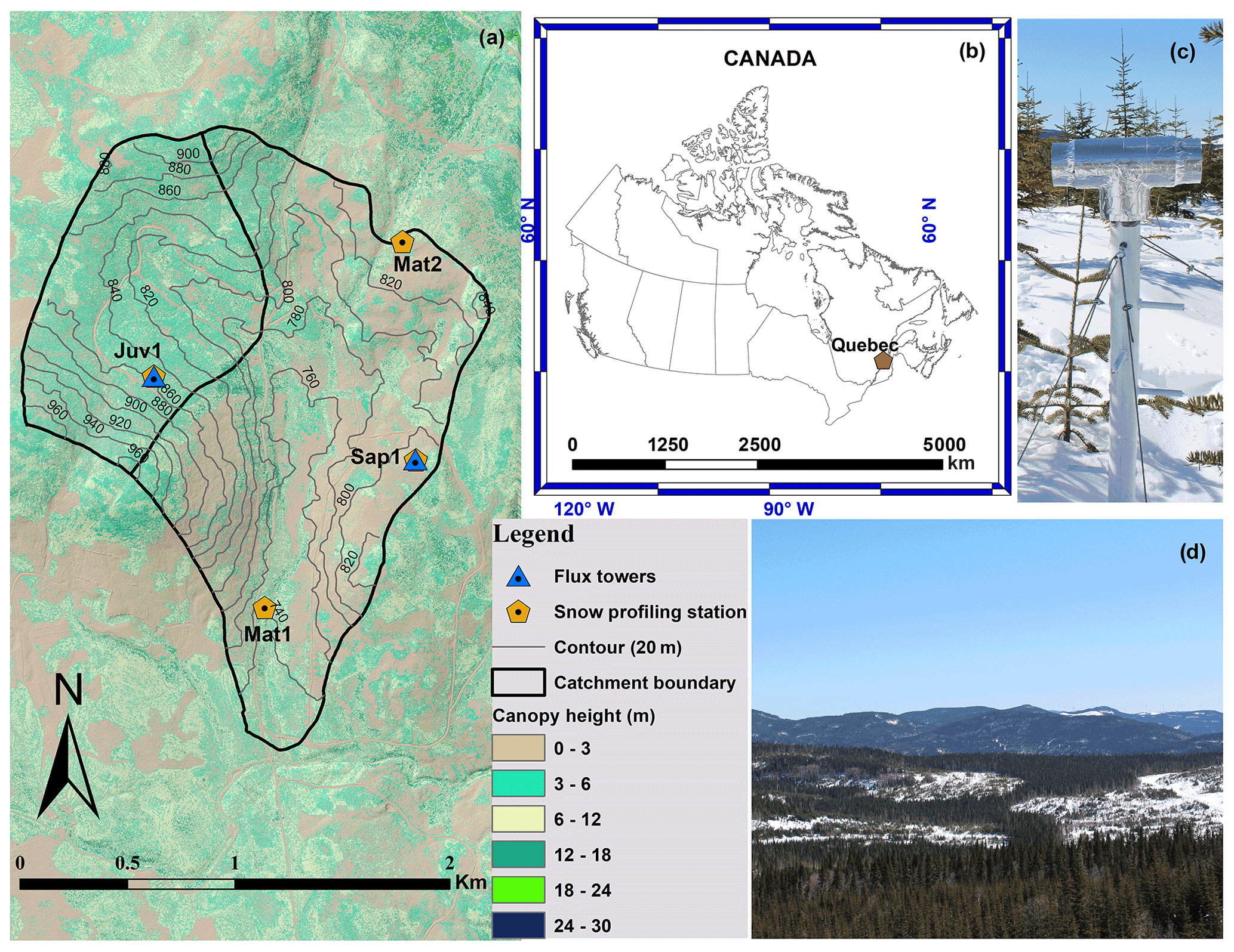
Figure 1Overview of the study area. (a) Basin 7 within BEREV showing the locations of the four study sites (note that elevations are in metres), where snowpit samples were collected and snow-profiling stations were installed, (b) the location of BEREV in eastern Canada, (c) the snow-profiling station installed at site Sap1, and (d) typical winter conditions at BEREV as seen from the flux tower at site Juv1.
Inspired by Lundquist and Lott (2008), we deployed an automated snow-profiling station at each location, composed of 18 T-type thermocouples vertically spaced 10 cm apart and an ultrasonic depth sensor (Judd Communications, USA). These stations report the local evolution of the snowpack temperature profile and height. An additional T-type thermocouple was enclosed in a radiation shield (Fig. 1c) 2 m above ground for simultaneous air temperature measurements.
Snowpit samples at 10 cm vertical intervals (temperature profile, depth, and density profile) were collected in the vicinity of the snow-profiling stations on a weekly basis from 17 January 2018 to 24 May 2018 (≈60 % of the snow cover period), enabling CC calculation following Eq. (1) and validation of the modelled output such as the snow water equivalent (SWE), snow density, and CC. Maintaining a weekly timeline was sometimes difficult due to uncontrollable circumstances such as freezing rain, rain-on-snow events, or even winter storms. During melt, from 21 April 2018 and on, it was impossible to reach all study sites because of reduced snow depths preventing the safe use of snowmobiles, except for site Juv1 that was more easily accessible from the main road. Snow-profiling stations malfunctioned occasionally (less than 1 % of the time), mostly in spring. Missing values were filled with snowpit observations. An exponential moving average procedure was implemented to reduce noise in automatic snow depth observations.
2.2 Construction of CC time series
The exercise of constructing 10 cm 30 min time series of the snowpack CC represents a certain challenge. On the one hand, it requires time series of the vertical profile of snow temperature, which is obtained from the snow-profiling stations. On the other hand, time series of the snow density profile are needed as well. This is where the main difficulty lies. A simple approach would be to interpolate the density values extracted from snowpits. However, our research site has the particularity of being very snowy and experiencing many episodes delivering >10 cm of fresh snow. Thus, such interpolation would be incomplete and error-prone given the limited number of snowpit surveys and their absence early in the season and towards the end of the melting period. Herein, we opted to produce multilayer time series of snow density thanks to CLASS bulk simulations complemented with empirical formulations, as detailed below. Note that Fig. 2 summarizes our methodological approach, describing the collection of weekly CC observations via snowpits (see Sect. 2.1) and the construction of continuous CC data every 30 min, which are the focus of the present section.
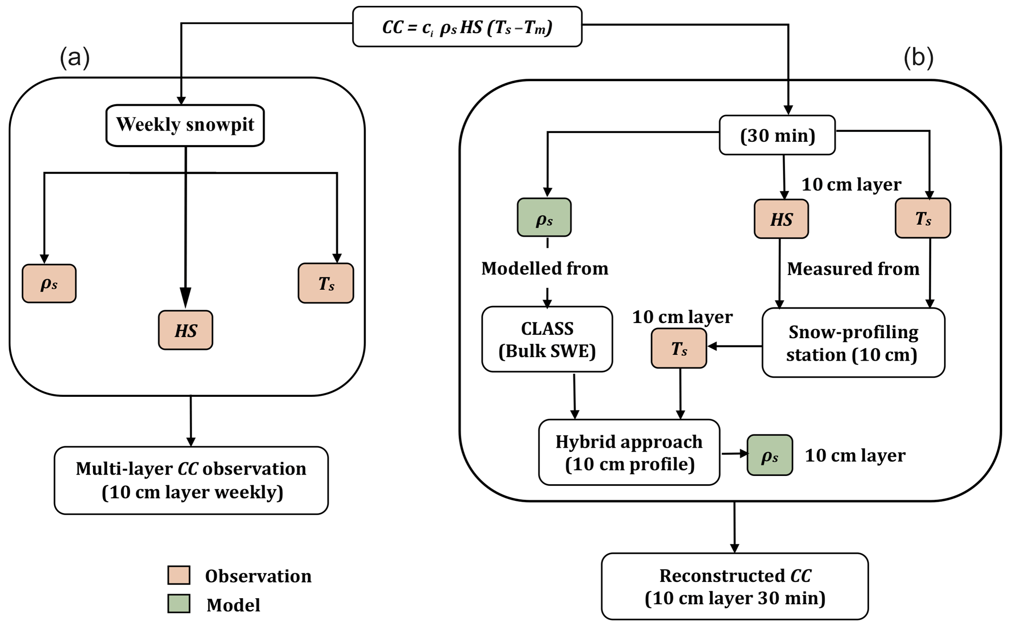
Figure 2Schematic representation of the methodology adopted in this study. The left column describes the acquisition of CC from weekly snowpits, while the right column describes the construction of continuous CC data every 30 min using an approach combining observations (orange cells) and modelling (green cells). ρs stands for snow density, HS for snow height, and Ts for snow temperature.
2.2.1 CLASS model
CLASS is a physically based land surface model that simulates the exchanges of water and energy between the Earth's surface and the atmosphere (Bartlett et al., 2006; Verseghy, 1991). It considers four distinct surface subareas: bare soil, canopy cover over bare soil, canopy with snow cover, and snow cover over bare soil (Bartlett and Verseghy, 2015; Verseghy et al., 2017). In this analysis, CLASS version 3.6 was used in offline mode and with a 30 min time step, ensuring an uninterrupted time series of the prognostic variables (Roy et al., 2013), hereby allowing the inclusion of multiple soil layers and accounts for snow interception, snow thermal conductivity, and snow albedo, as described in Bartlett et al. (2006). The following subsections describe the meteorological forcing data required to run CLASS and the methodology (CLASS + snow-profiling station) to produce single- and multi-layer time series of snow density, following Andreadis et al. (2009).
2.2.2 CLASS setup and forcing
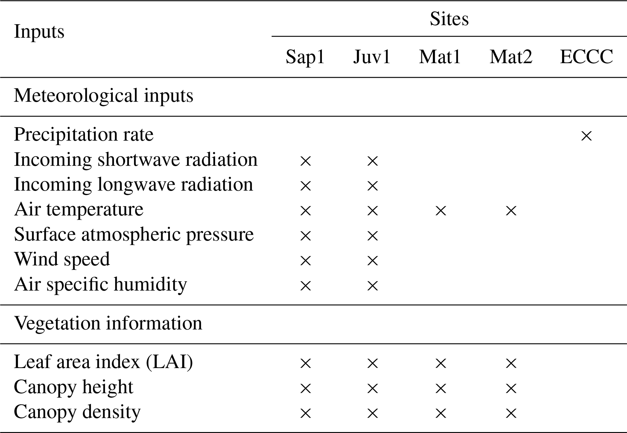
The meteorological inputs required to run CLASS include precipitation rate, wind speed, air specific humidity, incoming shortwave and longwave radiation, air temperature, and surface atmospheric pressure (Table 2). As CLASS is designed to explicitly consider the energy exchanges between the soil surface, vegetation, snowpack, and atmosphere, above-canopy meteorological forcings are used. The model accounts for local effects associated with the presence of a canopy (e.g. attenuation of incident radiation, etc.) and incorporates user-defined parameters such as tree height, canopy density, and leaf area index (Table 1).
Table 2Local availability of meteorological forcing data for use in CLASS simulations. Precipitation data are from Environment and Climate Change Canada (ECCC), weather station 7042388, located 4 km north of the BEREV.
These inputs serve to derive the energy budget components of the soil, vegetation, snowpack, and atmosphere. After solving the energy balance equation for the above-mentioned interfaces, the residual term (the available energy for melting or refreezing (Qm, in W m−2)) is derived. The amount of available melting/freezing energy next serves to compute the meltwater mass M given as
where M is the melt rate (m s−1), ρw is the density of water (kg m−3), Lf is the latent heat of fusion (J kg−1), and B is the thermal quality of the snowpack, which is defined as the energy required to melt a unit mass of snow divided by energy required by unit mass of ice at 0 ∘C, and is dimensionless. The melting or refreezing of the snowpack is associated with the available energy (Qm). A positive value of Qm might result in the melting of the snowpack, given that the available energy is large enough to eliminate the cold content and induce melt. However, a negative value of Qm contributes to the refreezing of liquid water or simply adds to the CC.
Precipitation rates were determined using a GEONOR weighing gauge equipped with a single Alter shield approximately 4 km north of the study area and were considered to be uniformly distributed throughout the catchment, which is a reasonable but imperfect assumption. Given the known wind-induced bias associated with this type of gauge (Pierre et al., 2019), a simple adjustment was applied. This adjustment involved twice-daily manual precipitation observations from a Double Fence Intercomparison Reference (DFIR) setup close by, as in Parajuli et al. (2020a). Although topography affects precipitation, no correction for height differences between stations was applied, as these are relatively small (<200 m). Vegetation parameters were extracted at each site from a lidar dataset. Wind speed, air specific humidity, shortwave and longwave radiation, and surface atmospheric pressure measurements were taken from flux towers at sites Sap1 and Juv1. Comparable data were unavailable at sites Mat1 and Mat2 (Table 2).
This study was carried out in a small experimental watershed with an area of 3.49 km2, where the sampling sites were close to one another (Fig. 1) but had distinct characteristics (Table 1). Given the similarity (more or less) in canopy structure, we opted to use the inputs recorded at site Juv1 to run CLASS simulations at sites that lacked direct measurements of meteorological variables (Table 2). Here we assumed negligible differences in the above-canopy inputs between sites Juv1, Mat1, and Mat2. The following subsection highlights the steps adopted to generate the multilayer density estimates needed to calculate the CC time series for all snow layers.
2.2.3 Reconstruction of multilayer snow density time series (a hybrid approach)
The empirical formulation described in Andreadis et al. (2009), based on Anderson (1976), is used to reconstruct multiple layer snow density estimates by combining the CLASS-derived SWE estimates (hereafter referred to as the hybrid procedure). Fresh-snow density follows the formulation from Brun et al. (1989), who developed the method using data collected in the French Alps. We initialized the density of fresh snow by imposing a minimum snow density of 76 kg m−3, based on available snowpit observations, and then using the following equation:
where ρf is the density of fresh snow (kg m−3), um is the wind speed (m s−1), and Ta is the air temperature (K). As snow undergoes compaction due to metamorphism and the increasing weight of overlying snow, density is assumed to increase according to the following rate:
where t is time (s), CRm is the snow compaction due to metamorphism (kg m−3 s−1), and CRo is the compaction due to the weight of overlying snow (kg m−3 s−1). CRm is then calculated as in Andreadis et al. (2009):
CRo is also calculated as in Andreadis et al. (2009):
where N s m−2 is the snow viscosity, c5=0.08 K−1, c6=0.021 m3 kg−1, and Ps (N s m−2) is the load pressure for each layer. The load pressure is defined as
where g is the acceleration due to gravity 9.8 m s−2, ρw is the density of water (kg m−3), SWEns and SWEs are the amount of new snow and the snow (derived from CLASS) within the snowpack layer (mm w.e.), respectively, and f is the empirical compaction coefficient taken as 0.6 (Andreadis et al., 2009).
3.1 Local meteorological conditions
Figure 3 displays daily air temperature and wind speed observations. The shaded zone and site-specific dots illustrate the temporal distribution of the manual snow surveys. Air temperature measurements were taken at 2 m above ground. Wind speed sensors were located 3 m and 2 m above ground at sites Sap1 and Juv1, respectively. To compensate for this height difference and enable fair comparisons between sites Sap1 and Juv1, wind speed measurements at site A1 were adjusted to a 2 m height, assuming a log profile. As expected, the sapling site (mean canopy of 1.8 m) experienced higher wind speeds (mean 1.3 m s−1) than the juvenile one (mean canopy of 8.1 m and mean wind speed of 0.12 m s−1). Air temperatures were homogenous from site to site, with average values of −6.1, −6.3, −6.9, and −6.5 ∘C at sites Sap1, Juv1, Mat1, and Mat2, respectively.
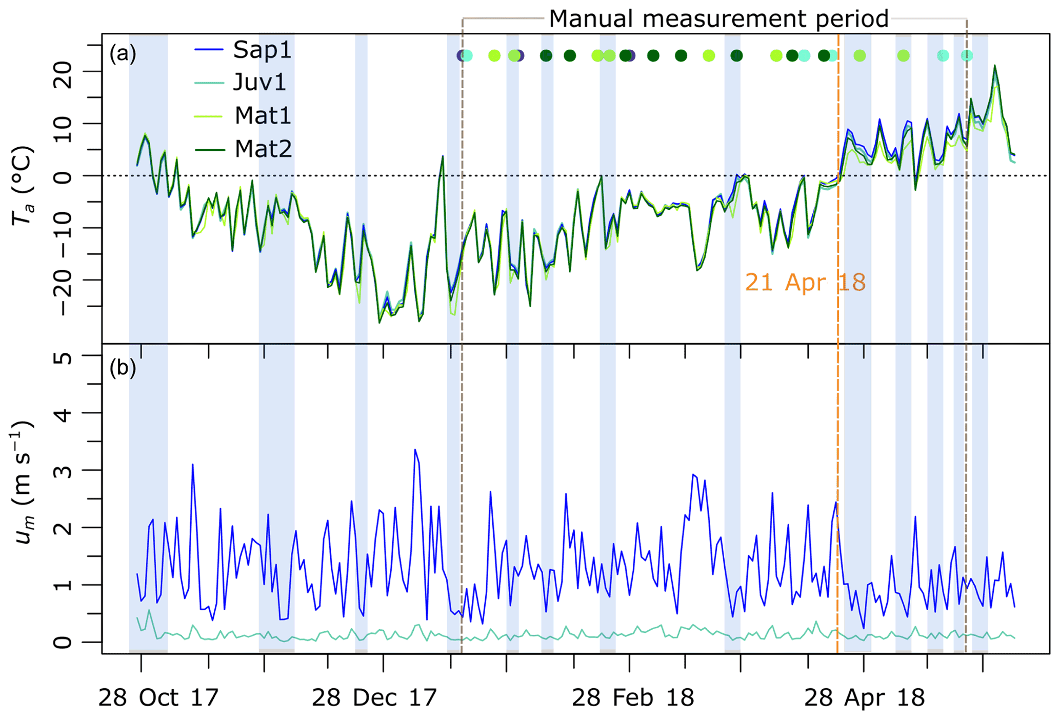
Figure 3(a) Daily 2 m air temperature (Ta) observations for all the study sites. (b) Daily 2 m wind speed (um) for sites Sap1 (sapling) and Juv1 (juvenile). Shaded areas denote periods of low wind speeds (<0.8 m s−1). Coloured points illustrate site-specific snowpit surveys. Spring melt started on 21 April 2018.
3.2 CC observations from snowpit surveys
Figure 4 illustrates 10 cm CC derived from the snowpit surveys. One has to sum up all the values of a single profile to find the total CC for a specific date. Variability in snow depth, mainly induced by contrasting canopy structure, is indicated in Fig. 4. When comparing layer-wise (10 cm) differences across our sites (Sap1, Juv1, Mat1, and Mat2), the lowest (−0.013 MJ m−2) and peak (−0.67 MJ m−2) CC both occurred at site Juv1. Unlike for spring melt, when CC is low and relatively uniform, the accumulation period portrays substantial layer-wise variability structured around three distinct layers. For instance, sites Sap1, Juv1, Mat1, and Mat2 reported 9, 15, 12, and 5 observations of CC that were below −0.35 MJ m−2. Note that the occurrence of a large magnitude of CC values was not always confined to the topmost layer, as the layer just beneath the top layer also exhibited such magnitude (see Fig. 4, week 10, site Mat1 at a snow depth of 106 cm, for example). However, the layers that are close to the ground experienced smaller magnitude of CC throughout the winter. Except for site Juv1 and Mat1, peak CC occurred in early February (Fig. 5 and Table 3), when the minimum daily air temperature fell to about −25 ∘C (Fig. 3). At that time, the magnitude of CC was highest at site Sap1, which also fostered the deepest snowpack (128 cm). Due to logistical constraints, we were unable to sample the Sap1 site on week 5, when all other sites appear to report one of the largest cold content amplitudes of the winter. Total CC time series highlight the variability of CC across the four study sites (Fig. 5). Site Juv1 attained its peak CC in mid-March (Table 3).
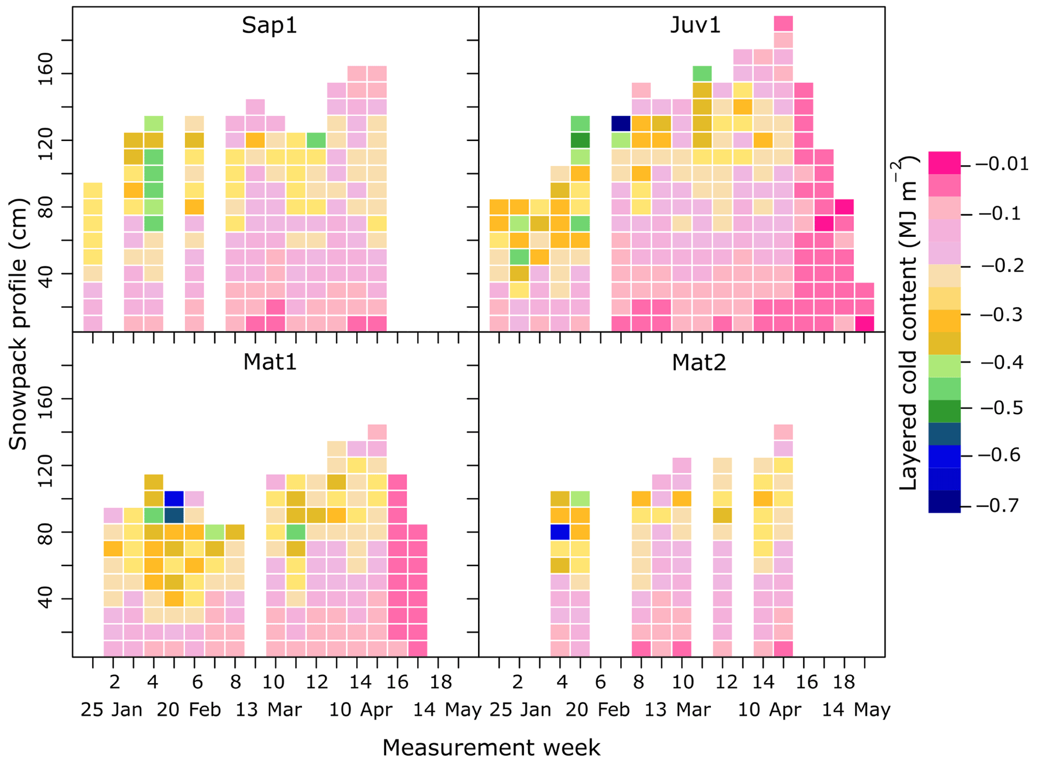
Figure 4Weekly 10 cm CC observations from snowpit surveys. The colour bar indicates CC values in MJ m−2.
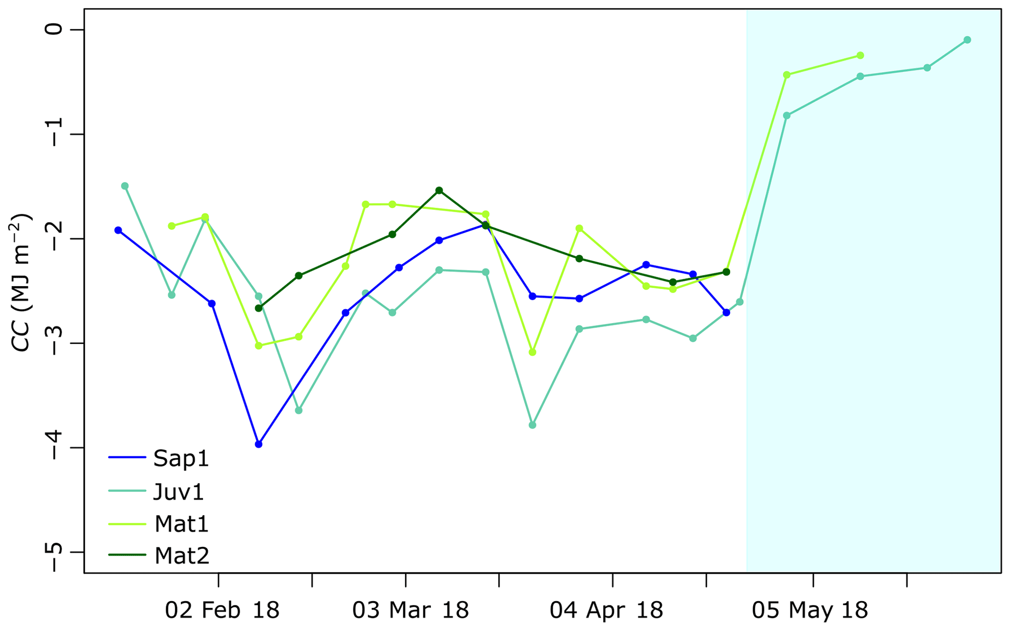
Figure 5Weekly snowpack total CC from snowpit surveys. The light blue shading represents active spring melt.
Table 3Peak total CC, date of occurrence, snow depth, mean tree height at the site, maximum snow depth, and mean total CC over a period of 15 weeks.

Overall, maximum snow depth occurred at site Juv1 (194 cm), which also experienced the largest magnitude of mean total CC (−2.62 MJ m−2), as a thicker snowpack can hold more CC (Table 3). For its part, Mat2 experienced the smallest maximum snow depth (142 cm) and the lowest magnitude of mean total CC (−2.15 MJ m−2). The CC difference across sites reached 0.47 MJ m−2 in total cold content, representing a variability of 20 %.
3.3 Analysis of reconstructed CC time series
3.3.1 Snow density modelling
A comparison of CLASS snow simulations and snowpit (manual) observations reveals that CLASS is reasonably able to simulate bulk snow density (Fig. 6; R2=0.71, Pbias =1.6 %), SWE (R2=0.64, Pbias = −17.1 %), and CC (R2=0.93, Pbias %). However, when comparing CLASS outputs, it appears that SWE is more underestimated than the snow density and CC (Fig. 6).

Figure 6Observed versus CLASS-simulated bulk values of SWE, snow density, and CC. R2 denotes the coefficient of determination, and Pbias (%) represents the percent bias.
Nevertheless, after confirming that CLASS was efficient in modelling bulk snow cover variables (Fig. 6), we moved forward with the next step in our methodology (Fig. 2). We adopted a hybrid procedure in which we reproduced a vertical structure following Andreadis et al. (2009). We compared layer-by-layer, simulated, and observed CC and snow density (Fig. 7) and determined that, on average (when all sites are considered), the empirical density and observed snow temperature yielded reasonable CC estimates (R2=0.54 and Pbias %). At each site, reasonable CC values were achieved over the entire profile (R2=0.67, 0.45, 0.58, and 0.29 and Pbias %, −19.7 %, −23.5 %, and −31.6 % at sites Sap1, Juv1, Mat1, and Mat2, respectively) (Fig. 8).
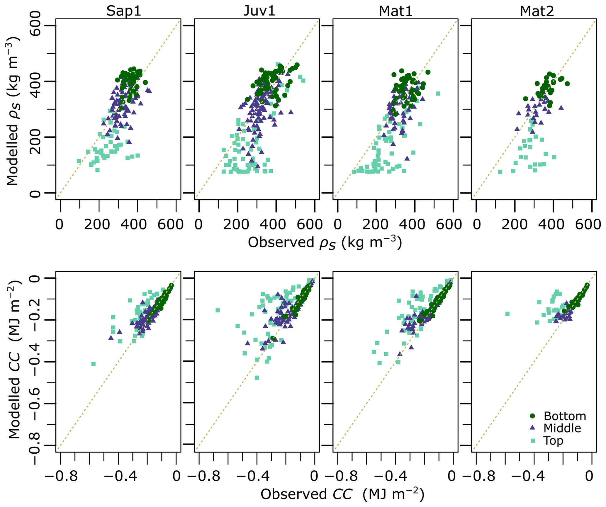
Figure 7Observed versus modelled snow density and CC derived from the empirical formulation described in Sect. 2.2.3 across the four sites. Snowpack layers are aggregated into three classes: top (upper 40 cm), bottom (lower 30 cm), and middle (remainder).
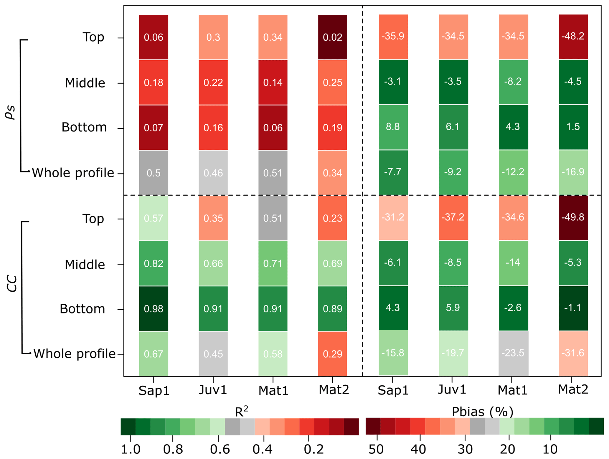
Figure 8Performance of CC and density simulations following the adopted hybrid procedure, coefficient of determination (R2, left), and percent bias (Pbias, right). Pbias colour bar applies to both positive and negative values.
As displayed in Fig. 8, we summarized the 10 cm layers into a three-layer scheme formed of the top (upper 40 cm), bottom (lower 30 cm), and middle layers (remainder). CCs for the top layer were more difficult to simulate (R2=0.57, 0.35, 0.51, and 0.23) than for the other two layers. Bottom-layer simulations were the most successful (R2=0.98, 0.91, 0.91, and 0.89). Density simulations over the entire profile behaved similarly ( 0.46. 0.51, and 0.34 and Pbias %, −9.2 %, −12.2 %, and −16.9 % at sites Sap1, Juv1, Mat1, and Mat2, respectively). The performance of density simulations, for each layer examined individually, was much less successful, mostly for the top layer (R2=0.06, 0.30, 0.34, and 0.02 and Pbias %, −34.5 %, −34.5 %, and −48.2 % for sites Sap1, Juv1, Mat1, and Mat2, respectively). However, snow density estimates had a low impact on CC performance, as described previously (Fig. 6). These results were deemed sufficient for moving forward with the fine-scale temporal analysis of the reconstructed CC.
3.3.2 Reconstructed CC time series
Figure 9 illustrates reconstructed multilayer 30 min CC time series. Although larger peaks (−6.9 MJ m−2 for site Sap1) and smaller average values (−1.8 MJ m−2 for site Juv1) are observed, the high-resolution CC time series that were derived using the hybrid procedure follows a pattern similar to the CC observations presented in Sect. 3.3.1 (Figs. 9 and 10a and Table 2). Additionally, sites with less vegetation (site Sap1) experienced higher peak CC than sites with mature forest (Mat2) (Fig. 9). Notably, the rain-on-snow episodes that occurred on 11 January, 20 February, and 30 March 2018 (thin vertical bands of low CC) were absent from the weekly series shown in Fig. 4. Sites Sap1, Mat1, and Mat2 had a shallower snowpack and the rainfall penetrated deeper, resulting in a reduced CC throughout the snowpack. Contrarily, at site Juv1, which had a deeper snowpack, similar rain penetration into the snowpack was only observed on 11 January 2018. All snowpacks became isothermal from 21 April 2018 onwards, indicating the onset of spring melt. Some cold spells during spring melt were also noticeable, especially for the shallower snowpacks (Sap1, Mat1, and Mat2).
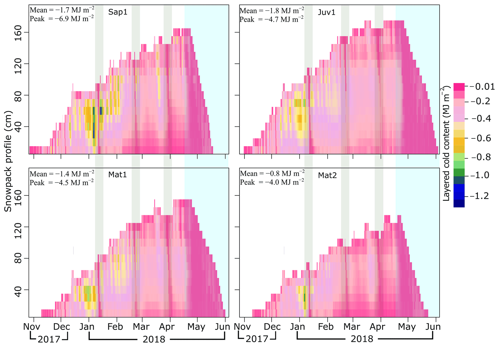
Figure 9Seasonal variability of 10 cm CC simulations stored at 30 min time intervals. The colour bar indicates CC values in MJ m−2. Light green shading represents rain-on-snow events, and light blue shading represents melt.
Due to differences in snow accumulation and melt patterns (Fig. 10), mostly induced by differences in vegetation (Table 1), there is noticeable site-to-site variability in CC (Fig. 9). The detailed variability of total CC across the four forested sites is presented in Fig. 10, along with snow depth. The magnitude of total CC at site Juv1 was larger than at Sap1 approximately 60 % of the time. At site Mat1, this fraction drops to 32 %.
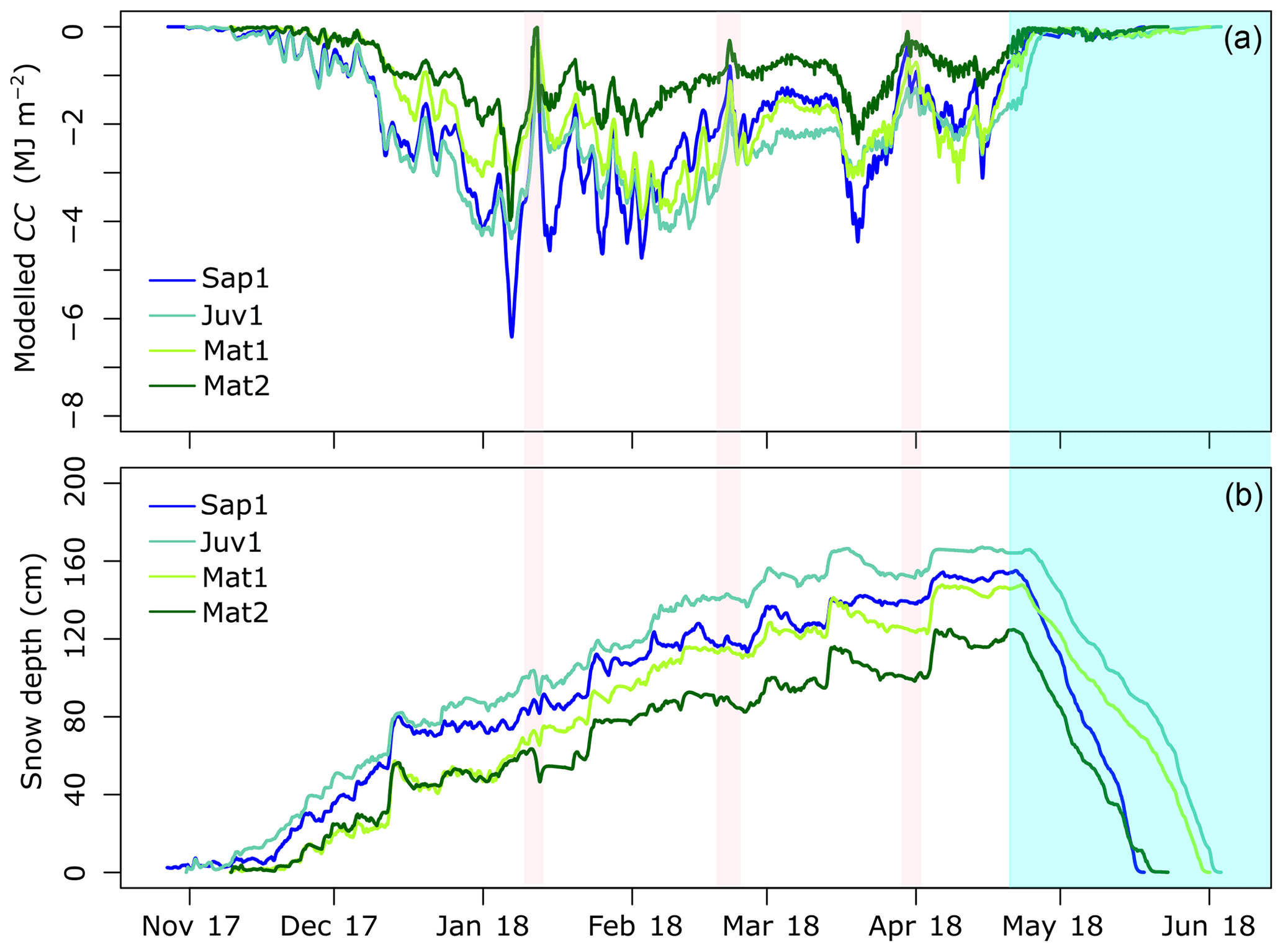
Figure 10(a) Total estimated CC from the reconstructed time series. An exponential moving average was applied for noise removal. (b) Snow depth observations. Spring melt period and rain-on-snow events are highlighted with light blue and light pink colours, respectively.
To shed light on site-to-site CC variability, Fig. 11 presents the average available energy Qm (W m−2) for melting or refreezing derived from CLASS. To facilitate the comparison, the figure divides the cold season into the winter accumulation (WA) period (excluding rain-on-snow events), the spring melting (SM) period, rain-on-snow (RS) events, and cold air pooling events, with low wind speed and nighttime air temperatures at site Mat1 smaller than at the other sites during the accumulation period (CP) (see also Fig. 3). During SM and RS, considerable amounts of energy were available, which might have depleted CC and initiated snowmelt. Conversely, WA and CP might have contributed to the refreezing of liquid water or to an increase in CC (Fig. 11). As expected, more melting energy was available at site Sap1 (lower vegetation) during SM (43.0 W m−2) and RS (46.0 W m−2). During WA, the mean of available melting/freezing energy was more or less similar at all sites and ranged from −6.6 W m−2 (Sap1) to −7.2 W m−2 (Juv1). Finally, during CP, the mean melting/refreezing energy was the smallest at Mat1 (−6.6 W m−2) and the largest at Juv1 (0.4 W m−2), the site with the highest elevation (849 m a.s.l.).

Figure 11Available mean melting/freezing energy at our sites. WA denotes the winter accumulation period, SM the spring melting period, RS the rain-on-snow events, and CP events with low wind speed coinciding with smaller air temperature at site Mat1.
Based on the Pearson correlation coefficient (r), we examined the relationship between CC and the snow density (ρs), snow depth (HS), snowpack temperature (Ts), and air temperature (Ta; Fig. 10). Snowpack temperature (r=0.83 and 0.69) and air temperature (r=0.56 and 0.66) exhibited a positive correlation, meaning that cold content magnitude increased as air temperature and snowpack temperatures decreased. Conversely, snow depth ( and −0.45) exhibited a negative correlation, whereas snow density (r=0.4 and 0.24) showed a weak relationship.
Next, we examined the relationship between each of the above-mentioned variables and CC at the individual sites. This was done to identify any trends in the site-wise relationship between CC and ρs HS, Ts, and Ta. A decreasing trend in the correlation coefficient (r) with increasing mean tree heights was observed when we examined the snow temperature and the reconstructed cold content for each site (r= 0.75, 0.69, 0.67, and 0.60 for sites Sap1, Juv1, Mat1, and Mat2, respectively). Beyond that relationship, we did not identify any site-wise trends between CC and the other variables, thereby suggesting a weak dependency on forest structure in the relationship between CC and other pertinent variables.
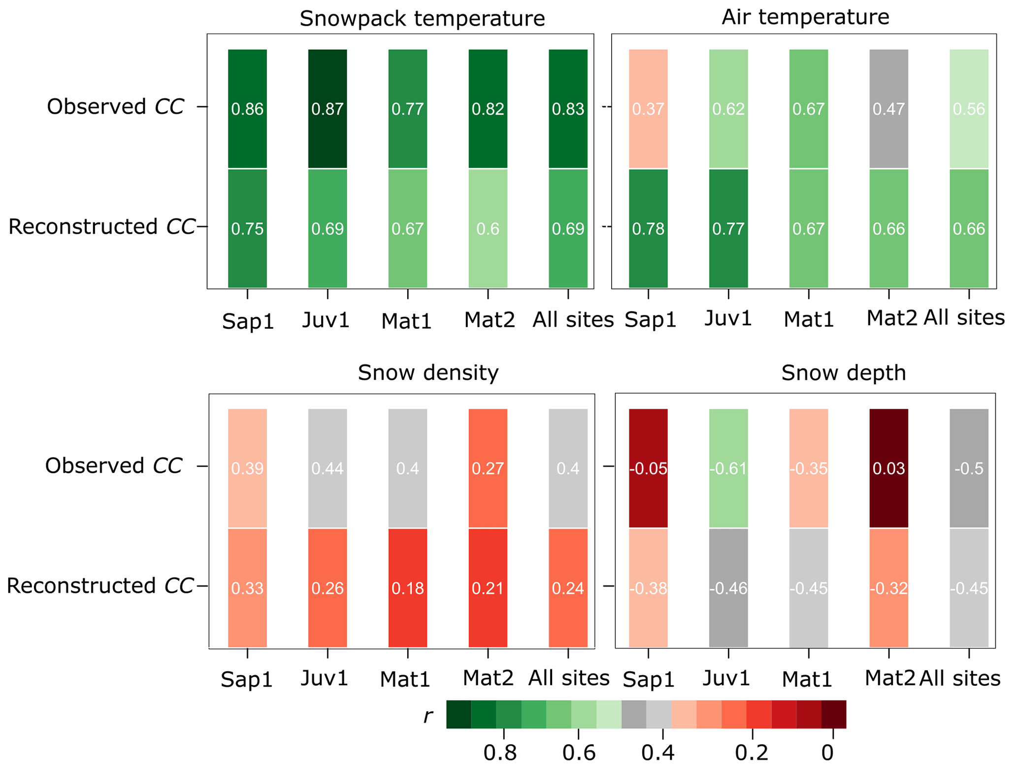
Figure 12Inter-relationship between CC and snow density, snow depth, snowpack temperature, and air temperature. The colour bar represents the absolute value of the Pearson correlation coefficient (r).
4.1 CC observations
The importance of snow mass on CC (total) at the study sites is highlighted in Fig. 5. As expected, a deeper snowpack is typically associated with higher CC. For instance, CC displayed a local maximum at all sites in February, but with greater amplitudes in the deeper Sap1 and Juv1 snowpacks. The same finding holds when CC is averaged over the 15-week period: Juv1 experienced more snow and higher CC, followed by Sap1. In both instances (peak and average CC conditions), a deeper snowpack led to larger magnitude of CC. In a similar study of alpine and subalpine snowpacks in the Rocky Mountains of Colorado, USA, Jennings et al. (2018) reported peak CC to be 2.6 times greater for the alpine snowpack than for the subalpine location, which they mostly attributed to the higher SWE accumulation at the alpine site. However, Jennings et al. (2018) also noted that colder temperatures (up to 4 ∘C) led to higher CC at their alpine site.
In early February (during peak CC conditions at two of the sites), the snow depth difference between sites Sap1 and Juv1 was very small (Table 3). Nonetheless, Sap1 exhibited higher CC than Juv1 (Fig. 5). This is because in addition to snow depth, CC values depend on the density and temperature of the snow (Fig. 12). The higher peak CC found at site Sap1 can be explained by the higher snow density that is typically associated with higher wind velocities (Vionnet et al., 2012) and wind-speed-induced densification. Also, as illustrated in Fig. 3, site Sap1 was windier than Juv1. This is expected, as wind speed is lower within forest canopies (Davis et al., 1997; Harding and Pomeroy, 1996), such as those in site Juv1. Finally, as explained in Sect. 4.1, the Sap1 site is more exposed to atmospheric conditions without the protective effect of the canopy, making it more likely to respond to cold snaps for example.
4.2 CLASS performance
Gaps between weekly snowpit surveys failed to capture short-lived events such as warm and cold spells or rain-on-snow events. In an attempt to produce higher-frequency CC time series, we used the CLASS land surface model to simulate 30 min bulk snow density and SWE. Based on our findings, CLASS successfully estimated snow density and CC, while underpredicting SWE (Fig. 6).
Alves et al. (2020), who operated CLASS on the same experimental watershed as in this study, reported an overestimation in the upper quantile of the latent heat flux. Interestingly, a similar pattern was reported for other Canadian boreal forest sites. Similarly, Parajuli et al. (2020a) explored a simple temperature-index (TI) model, again at the same sites. They found that the inclusion of snow sublimation led to improvements in their model performance. Based on these recent studies, it seems fair to conclude that the overestimation of latent heat fluxes by CLASS could lead to SWE underestimation. The precipitation biases reported in the methodology section could also have impacted SWE estimation. It is equally important to point out that the single-layer representation of snowpack processes by CLASS stands out as a major shortcoming. Given the limitations of bulk estimations, which are often too broad to properly describe all snowpack processes (Roy et al., 2013), several studies have opted for multilayer snow models (Brun et al., 1997; Lehning et al., 2002; Vionnet et al., 2012). Whether the model is single- or multi-layer, a certain degree of uncertainty will persist when modelling snowpack processes (Jennings et al., 2018; Raleigh et al., 2015; Alves et al., 2020). Given the prevalence of biases in the snow modelling chain, we feel confident enough to use CLASS-estimated SWE to derive multilayer snow density.
4.3 Reconstructed CC time series
For CC reconstruction this study explored the (simpler) hybrid procedure proposed by Andreadis et al. (2009). Using this method, we generated reasonable snow density (10 cm vertical layers) values to support the derivation of multilayer CC time series that are better able to capture short-lived events (Fig. 9). To better visualize the variability of snow density and cold content estimates, we aggregated the snowpack (10 cm layer) into top, middle, and bottom snow layers (Fig. 8). One should keep in mind though that all results presented in Sect. 3.3.2 are based on 10 cm vertical slices. As shown in Fig. 7, snow density was less well modelled for the top layer than for the other two layers, which obviously also affected the CC estimates (Fig. 8). One of the challenges of snow modelling is the estimation of fresh-snow density. Russell et al. (2020) explored a range of fresh-snow density formulations and concluded that a constant value of 100 kg m−3 provided a better outcome than most empirical formulations. In Fig. 13, we compare observations of the top 10 cm snow density versus model outputs from three common empirical methods: Diamond–Lowry (Russell et al., 2020), Hedstrom–Pomeroy (Hedstrom and Pomeroy, 1998), and Brun (Shrestha et al., 2010; Vionnet et al., 2012) (Fig. 12). As proposed in Russell et al. (2020), we also explored a constant fresh-snow density of 100 kg m−3. Note that empirical methods are used to derive fresh-snow density only, and in cases where the observations are taken more than 24 h after a precipitation event (Fig. 13b), snow metamorphism must be taken into account in order to have a fair comparison between models and observations. Thus, to account for snow metamorphism, we resorted to Eq. (5) and then derived snow density.
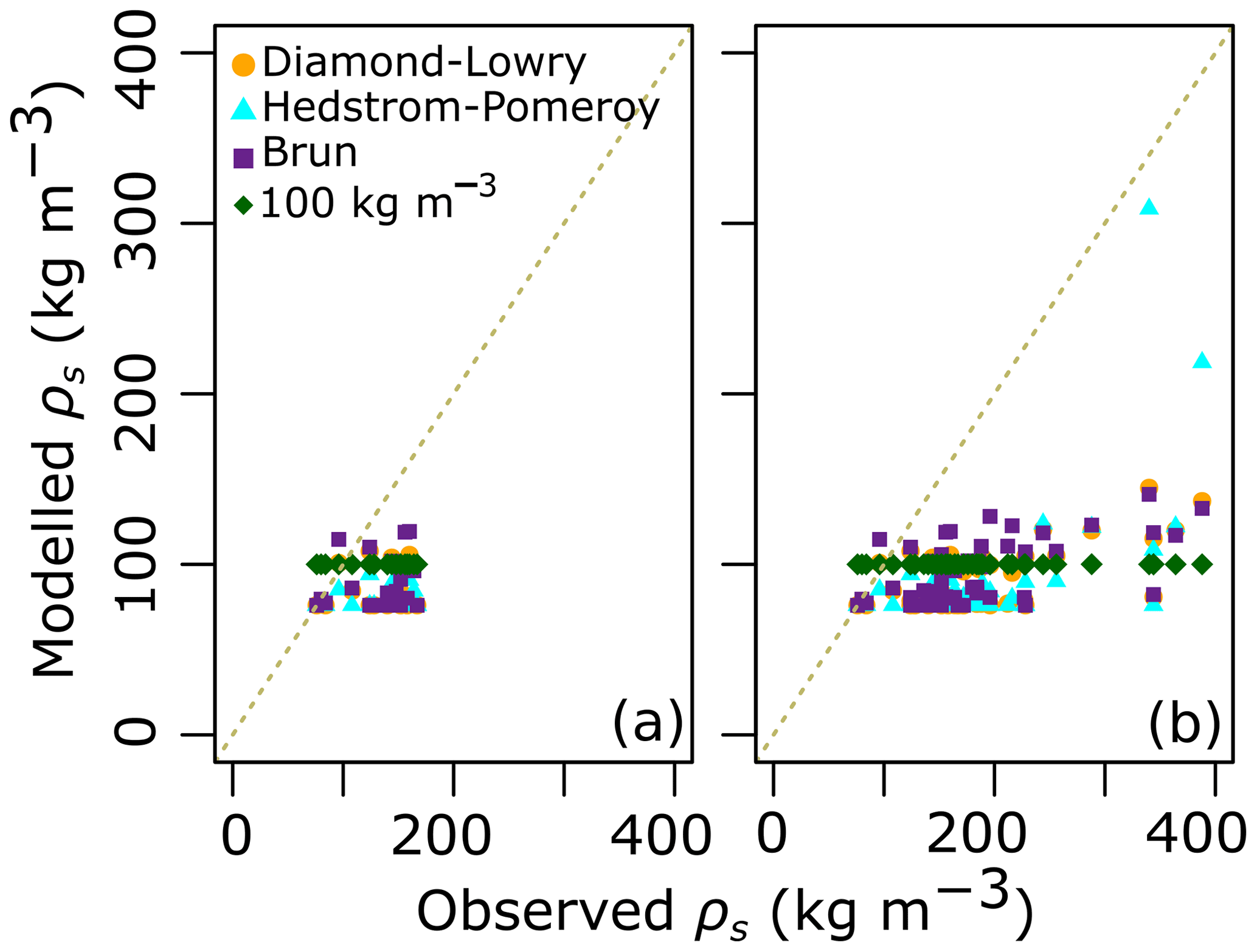
Figure 13Top 10 cm snow density derived from different empirical methods. (a) Observed versus modelled fresh-snow density (<24 h since last snowfall); (b) observed versus modelled snow density including both fresh and snow density after metamorphism based on Eq. (5).
All four methods performed poorly (Diamond–Lowry, Pbias % and R2=0.23; Hedstrom–Pomeroy, Pbias % and R2=0.25; Brun, Pbias 50.2 % and R2=0.18; and constant 100 kg m−3, Pbias 48.8 % and R2=0.11), largely underestimating snow density (Fig. 8b). One possible cause of this underestimation is related to the presence of a canopy. It is well known that intercepted snow can stay in place for several days to months (DeWalle and Rango, 2008). Such snow can densify within the canopy and eventually unload, thereby transforming the top-layer density underneath. In addition, the intercepted snow could be heated by radiation incident on the canopy. In doing so, local melting could be observed, resulting in dripping and an increase in the density of the top snow layers. It is possible that CLASS does not capture this phenomenon well. In agreement with both hypotheses, as noted in Figs. 7 and 8, top snow density estimated at the site with the shortest vegetation (Sap1), where there is little interception, was better than at the other sites. In a slightly different context, Raleigh and Small (2017) concluded that snow density modelling was a major source of uncertainty when studying catchment SWE derived from remotely sensed data.
The canopy not only intercepts some of the precipitation, but it also acts as a buffer on energy exchanges between the snowpack and the atmosphere. Indeed, the site with the shortest vegetation, Sap1, has the largest peak CC (Table 3 and Fig. 9), even if it is not the site with the deepest snow cover. When looking at the whole winter, we note that site Juv1 experienced more snow and a greater magnitude of total CC than Sap1 (Fig. 10). Delving into the reasons for this difference between the two sites, we find that the absence of a well-defined forest canopy appears to lead to a more responsive snow cover to meteorological forcing at site Sap1. The prevalence of higher wind speeds at site Sap1 intensifies turbulent sensible heat fluxes and thus favours the loss of heat from the snow cover in cold periods such as the one corresponding to the peak CC. Yet, this snow cover responsiveness at the Sap1 site does not guarantee that it has the greatest total mean CC, here observed at the site Juv1. Actually, if winds increase the sensible heat flux at Sap1, they also favour the lateral transport of snow. The absence of a well-defined canopy also means greater incoming shortwave radiation. In fact, our CLASS simulations reveal that the average of net shortwave radiation was greater by 4.6 W m−2 at Sap1 than at Juv1. Thus, wind scoured thinning combined with radiation enhanced ablation resulted in less snow accumulation at site Sap1 and, as such, a smaller mean total CC. This is also the reason why the magnitude of CC was higher at site Juv1 than at Sap1, i.e. 60 % of the time.
For site Mat1, the magnitude of CC was higher than at Sap1 32 % of the time, beginning in early February and continuing through the rest of the study period (Fig. 10). Most of the time, the measured snow depth at site Mat1 was also shallower than at site Sap1. We hypothesize that cold air pooling might explain this phenomenon. During stable atmospheric boundary layer conditions, with weak synoptic forcing, there is reduced wind flow. This results in thermal decoupling in the valley depression, which favours the formation of a cold air pool (Fujita et al., 2010; Mott et al., 2016). This is substantiated by the rapid cooling of near-surface air within the valley depression, typically at night or early in the morning (Smith et al., 2010). Here, in Fig. 3, we assumed that the reduced wind speed coincides with the rapidly cooling near-surface temperatures (see the shaded regions) as stable atmospheric conditions prevail. During these periods, Mat1 experienced cooler air temperature than the other sites. The mean energy available for melting or refreezing at Mat1 is also smaller than for the other sites (Fig. 11). As mentioned above, smaller melt/refreeze energy contribute to the accumulation of CC or the refreezing of liquid water present in the snowpack.
The site with the tallest trees, Mat2, has the lowest mean CC (Table 3 and Fig. 9). This is partly due to a lower snow height on the ground (more interception), the barrier effect of the canopy on incoming radiation, and enhanced longwave radiation within forest. Also, this site experienced very few occurrences where CC was larger than at site Sap1 (1 % of the data) and all of them during spring melt or rain-on-snow events. It is obvious because the rain-on-snow events contribute the addition of warm sensible heat to the snowpack (Marks et al., 1998; DeWalle and Rango, 2008). Any heat addition results in the elimination of some snowpack CC and drives destructive metamorphism to initiate melt (Seligman et al., 2014). For these periods, the taller tree at site Mat2 intercepts more rain than at site Sap1. This is the reason why the average of available melt energy was smaller at site Mat2 by 9.7 (rain-on-snow events) and 8.4 W m−2 (spring melting period) than at Sap1 (Fig. 11). Less availability of melt energy translates into smaller depletion of snowpack CC. Thus, only during the rain-on-snow and spring melt, one may notice more snowpack CC at site Mat2 than at Sap1.
Initially, based on Figs. 3 and 10, snow depth and air temperature appear to influence CC distribution across study sites. However, observed snowpack CC and simulated snowpack CC at all sites were strongly (positively) correlated with snowpack temperature and air temperature and weakly correlated with the snow density and snow depth values (Fig. 12). It should be noted that CC values at all sites only showed negative correlations with snow depth (Fig. 12). When translating the relationship between CC and the depth of the snowpack, one must understand that there is an increase in the magnitude of CC with an increase in snow depth. This is because the value of CC is expressed negatively while snow depth is always positive. Based on CC observations and the hybrid procedure, we were able to identify a relationship between the mean CC and the tree height (Table 3 and Fig. 9). However, we were unable to report any trends in the site-wise relationship between CC and the above-mentioned variables (Fig. 12). Conversely, Jennings et al. (2018) attempted to establish a relationship between CC development and the cumulative mean of air temperature across the alpine and subalpine sites in the Rocky Mountains in Colorado, USA, but were unsuccessful.
4.4 Sources of uncertainty
Several errors and biases could arise due to poor data quality and modelling deficiencies, thereby affecting the snowmelt models (Parajuli et al., 2020a; Raleigh et al., 2015, 2016; Rutter et al., 2009). For instance, Jennings et al. (2018) applied the SNOWPACK multilayer model and reported an overestimation in fresh-snow temperature. As reported in the present study, CC depends heavily on snowpack temperature (Fig. 12). Any biases arising due to inaccurate derivation of snow temperature might affect CC estimations. The quality of model inputs also influences model performance. For instance, precipitation inputs extracted 4 km north from present study sites were used to drive CLASS simulations, which neglects the presence of small-scale spatial variability in precipitation. Also, sites Sap1 and Juv1 benefitted from local flux tower measurements, but such direct measurements were not available for sites Mat1 and Mat2, for which many assumptions were necessary in order to create missing input time series. This problem has also been observed in several other studies (e.g. Pomeroy et al., 2007; Qi et al., 2017). Important snowpack properties beyond just CC, such as thermal conductivity (Oldroyd et al., 2013) and snow interception (Hedstrom and Pomeroy, 1998), also need to be further addressed. As mentioned in Sect. 4.2, snow density estimation presents a considerable challenge when implementing a multilayer snowpack model (Fig. 7). Therefore, future research that utilizes the physically based snow model and describes the internal snowpack processes should focus on improving snow density estimations.
The purpose of this study was to document the spatial variability of CC in a humid boreal forest, using detailed measurements supplemented by physically based and empirical model outputs. The studied boreal forest is characterized by a non-uniform stand structure that led to site-to-site variations in the 10 cm weekly observations of CC. The two sites with lower vegetation had greater snow accumulation and larger peaks in total CC relative to the sites with taller vegetation over the 15 weeks.
The Canadian Land Surface Scheme model was coupled with complementary empirical formulations to construct bulk, followed by 10 cm, 30 min snow density time series. Both CLASS and the empirical formulations supplied reasonable snow density and CC estimates. When the latter 10 cm time series were split into three layers, the bottom and the middle layers also resulted in reasonable simulations. However, modelling of the top layer was not as successful. The constructed time series were used to illustrate the influence of phenomena that are not detectable when only snowpit data are used, such as rain-on-snow episodes or the formation of cold air pools at the bottom of the valley.
We used the Pearson correlation coefficient (r) to identify the role of pertinent variables (snow density, snowpack temperature, snow depth, and air temperature) that affect the distribution of CC at our boreal forest sites. Snowpack and air temperature appeared to be highly influential on CC distribution compared to the depth and the density of the snowpack. Our study was supported by 30 min time step time series of 10 cm snow temperature profiles and bias-corrected precipitation inputs. The inclusion of such inputs helped us to reduce errors and biases. This study also highlighted the uncertainty associated with fresh-snow density estimates when simulating physically based snowmelt models.
The data that support the findings in this study are available upon request to the main author.
AP and DFN (occasionally) extracted the data from the field. AP, DFN, and FA designed the study. AP wrote the manuscript and analyzed the data. DFN and FA provided constructive feedback to improve the quality of the manuscript. MA performed CLASS simulations.
The contact author has declared that neither they nor their co-authors have any competing interests.
Publisher's note: Copernicus Publications remains neutral with regard to jurisdictional claims in published maps and institutional affiliations.
This research is a part of the EVAP project which was funded by the Natural Sciences and Engineering Council of Canada (NSERC), Ouranos (Consortium on Regional Climatology and Adaptation to Climate Change), Hydro-Québec, Environment and Climate Change Canada, and Québec Ministère du Développement Durable, de l’Environnement et de la Lutte Contre les Changements Climatiques through grant no. RDCPJ-477125-14. We would like to express our sincere gratitude to Sylvain Jutras for kindly providing the necessary sensors and support for managing the logistics of the field experiment. We conducted two successful winter campaigns, thanks to the generous support from André Desrochers, who provided a snowmobile. The authors would like to thank François Larochelle and Martine Lapointe for providing some of the equipment and helping in the design of the snow-profiling stations. Our study would have been incomplete without support from Annie-Claude Parent, who participated in the harsh winter field campaign, managed the necessary logistics, and helped conduct the field work. We would like to express our deepest gratitude to Benjamin Bouchard and Médéric Girard, who assisted in data collection. The authors are indebted to the Montmorency Forest staff, including Robert Côté and Charles Villeneuve, who provided generous support for managing the logistics throughout the study area. We thank group members Bram Hadiwijaya, Pierre-Erik Isabelle, Oliver S. Schilling, Judith Fournier, Alicia Talbot Lanciault, Georg Lackner, Carine Poncelet, Amandine Pierre, Guillaume Hazemann, Marco Alves, Adrien Pierre, and Antoine Thiboult; interns Fabien Gaillard Blancard, Jonas Götte, and Kelly Proteau; and PEGEAUX members, who participated in the challenging winter field campaign.
This research has been supported by the Québec Ministère du Développement Durable, de l'Environnement et de la Lutte Contre les Changements Climatiques (grant no. RDCPJ-477125-14).
This paper was edited by Carrie Vuyovich and reviewed by Keith Jennings and one anonymous referee.
Alves, M., Nadeau, D. F., Music, B., Anctil, F., and Parajuli, A.: On the performance of the Canadian Land Surface Scheme driven by the ERA5 reanalysis over the Canadian boreal forest, J. Hydrometeorol., 21, 1383–1404, https://doi.org/10.1175/jhm-d-19-0172.1, 2020.
Anderson, E. A.: A point energy and mass balance model of a snow cover, US Department of Commerce, National Oceanic and Atmospheric Administration, National Weather Service, Office of Hydrology, Washington DC, USA, 1976.
Andreadis, K. M., Storck, P., and Lettenmaier, D. P.: Modeling snow accumulation and ablation processes in forested environments, Water Resour. Res., 45, 1–13, https://doi.org/10.1029/2008WR007042, 2009.
Barnett, T. P., Adam, J. C., and Lettenmaier, D. P.: Potential impacts of a warming climate on water availability in snow-dominated regions, Nature, 438, 303–309, https://doi.org/10.1038/nature04141, 2005.
Bartlett, P. A. and Verseghy, D. L.: Modified treatment of intercepted snow improves the simulated forest albedo in the Canadian Land Surface Scheme, Hydrol. Process., 29, 3208–3226, https://doi.org/10.1002/hyp.10431, 2015.
Bartlett, P. A., MacKay, M. D., and Verseghy, D. L.: Modified snow algorithms in the Canadian land surface scheme: Model runs and sensitivity analysis at three boreal forest stands, Atmos. Ocean, 44, 207–222, https://doi.org/10.3137/ao.440301, 2006.
Brun, E., Martin, E., Simon, V., Gendre, C., and Coleou, C.: An energy and mass model of snow cover suitable for operational avalanche forecasting, J. Glaciol., 35, 333–342, https://doi.org/10.1017/S0022143000009254, 1989.
Brun, E., Martin, E., and Spiridonov, V.: Coupling a multi-layered snow model with a GCM, Ann. Glaciol., 25, 66–72, https://doi.org/10.1017/s0260305500013811, 1997.
Davis, R. E., Hardy, J. P., Ni, W., Woodcock, C., McKenzie, J. C., Jordan, R., and Li, X.: Variation of snow cover ablation in the boreal forest: A sensitivity study on the effects of conifer canopy, J. Geophys. Res., 102, 29389–29395, https://doi.org/10.1029/97JD01335, 1997.
DeWalle, D. R. and Rango, A.: Principles of snow hydrology, 1st ed., Cambridge University Press, New York, 1–410, ISBN 978 0 521 82362 3, 2008.
Essery, R., Morin, S., Lejeune, Y., and Ménard, C. B.: A comparison of 1701 snow models using observations from an alpine site, Adv. Water Resour., 55, 131–148, https://doi.org/10.1016/j.advwatres.2012.07.013, 2013.
Fujita, K., Hiyama, K., Iida, H., and Ageta, Y.: Self-regulated fluctuations in the ablation of a snow patch over four decades, Water Resour. Res., 46, 1–9, https://doi.org/10.1029/2009WR008383, 2010.
Gouttevin, I., Lehning, M., Jonas, T., Gustafsson, D., and Mölder, M.: A two-layer canopy model with thermal inertia for an improved snowpack energy balance below needleleaf forest (model SNOWPACK, version 3.2.1, revision 741), Geosci. Model Dev., 8, 2379–2398, https://doi.org/10.5194/gmd-8-2379-2015, 2015.
Harding, R. J. and Pomeroy, J. W.: The energy balance of the winter boreal landscape, J. Climate, 9, 2778–2787, https://doi.org/10.1175/1520-0442(1996)009<2778:TEBOTW>2.0.CO;2, 1996.
Hedstrom, N. R. and Pomeroy, J. W.: Measurements and modelling of snow interception in the boreal forest, Hydrol. Process., 12, 1611–1625, https://doi.org/10.1002/(SICI)1099-1085(199808/09)12:10/11<1611::AID-HYP684>3.0.CO;2-4, 1998.
Isabelle, P. E., Nadeau, D. F., Asselin, M. H., Harvey, R., Musselman, K. N., Rousseau, A. N., and Anctil, F.: Solar radiation transmittance of a boreal balsam fir canopy: Spatiotemporal variability and impacts on growing season hydrology, Agric. For. Meteorol., 263, 1–14, https://doi.org/10.1016/j.agrformet.2018.07.022, 2018.
Isabelle, P. E., Nadeau, D. F., Rousseau, A. N., Anctil, F., Jutras, S., and Music, B.: Impacts of high precipitation on the energy and water budgets of a humid boreal forest, Agric. For. Meteorol., 280, 1–13, https://doi.org/10.1016/j.agrformet.2019.107813, 2020.
Jennings, K. S., Kittel, T. G. F., and Molotch, N. P.: Observations and simulations of the seasonal evolution of snowpack cold content and its relation to snowmelt and the snowpack energy budget, The Cryosphere, 12, 1595–1614, https://doi.org/10.5194/tc-12-1595-2018, 2018.
Jost, G., Moore, R. D., Smith, R., and Gluns, D. R.: Distributed temperature-index snowmelt modelling for forested catchments, J. Hydrol., 420–421, 87–101, https://doi.org/10.1016/j.jhydrol.2011.11.045, 2012.
Koivusalo, H., Heikinheimo, M., and Karvonen, T.: Test of a simple two-layer parameterisation to simulate the energy balance and temperature of a snow pack, Theor. Appl. Climatol., 70, 65–79, https://doi.org/10.1007/s007040170006, 2001.
Lehning, M., Bartelt, P., Brown, B., and Fierz, C.: A physical SNOWPACK model for the Swiss avalanche warning Part III: Meteorological forcing, thin layer formation and evaluation, Cold Reg. Sci. Technol., 35, 169–184, https://doi.org/10.1016/S0165-232X(02)00072-1, 2002.
Lundquist, J. D. and Lott, F.: Using inexpensive temperature sensors to monitor the duration and heterogeneity of snow-covered areas, Water Resour. Res., 44, 1–6, https://doi.org/10.1029/2008WR007035, 2008.
Mahat, V. and Tarboton, D. G.: Canopy radiation transmission for an energy balance snowmelt model, Water Resour. Res., 48, 1–16, https://doi.org/10.1029/2011WR010438, 2012.
Marks, D. and Winstral, A.: Comparison of snow deposition, the snow cover energy balance, and snowmelt at two sites in a semiarid mountain basin, J. Hydrometeorol., 2, 213–227, https://doi.org/10.1175/1525-7541(2001)002<0213:COSDTS>2.0.CO;2, 2001.
Marks, D., Kimball, J., Tingey, D., and Link, T.: The sensitivity of snowmelt processes to climate conditions and forest cover during rain-on-snow: a case study of the 1996 Pacific Northwest flood, Hydrol. Process., 12, 1569–1587, https://doi.org/10.1002/(SICI)1099-1085(199808/09)12:10/11<1569::AID-HYP682>3.0.CO;2-L, 1998.
Molotch, N. P., Brooks, P. D., Burns, S. P., Litvak, M., Monson, R. K., McConnell, J. R., and Musselman, K. N.: Ecohydrological controls on snowmelt partitioning in mixed-conifer sub-alpine forests, Ecohydrology, 2, 129–142, https://doi.org/10.1002/eco.48, 2009.
Mosier, T. M., Hill, D. F., and Sharp, K. V.: How much cryosphere model complexity is just right? Exploration using the conceptual cryosphere hydrology framework, The Cryosphere, 10, 2147–2171, https://doi.org/10.5194/tc-10-2147-2016, 2016.
Mott, R., Paterna, E., Horender, S., Crivelli, P., and Lehning, M.: Wind tunnel experiments: cold-air pooling and atmospheric decoupling above a melting snow patch, The Cryosphere, 10, 445–458, https://doi.org/10.5194/tc-10-445-2016, 2016.
Musselman, K., Molotch, N., and Brooks, P.: Effect of vegetation on snow accumulation and ablation in a mid-latitude sub-alpine forest, Hydrol. Process., 22, 2267–2274, https://doi.org/10.1002/hyp.7050, 2008.
Oldroyd, H. J., Higgins, C. W., Huwald, H., Selker, J. S., and Parlange, M. B.: Thermal diffusivity of seasonal snow determined from temperature profiles, Adv. Water Resour., 55, 121–130, https://doi.org/10.1016/j.advwatres.2012.06.011, 2013.
Parajuli, A., Nadeau, D. F., Anctil, F., Schilling, O. S., and Jutras, S.: Does data availability constrain temperature-index snow model? A case study in the humid boreal forest, Water, 12, 1–22, https://doi.org/10.3390/w12082284, 2020a.
Parajuli, A., Nadeau, D. F., Anctil, F., Parent, A.-C., Bouchard, B., Girard, M., and Jutras, S.: Exploring the spatiotemporal variability of the snow water equivalent in a small boreal forest catchment through observation and modelling, Hydrol. Process., 34, 2628–2644, https://doi.org/10.1002/hyp.13756, 2020b.
Pierre, A., Jutras, S., Smith, C., Kochendorfer, J., Fortin, V., and Anctil, F.: Evaluation of catch efficiency transfer functions for unshielded and single-alter-shielded solid precipitation measurements, J. Atmos. Ocean. Technol., 36, 865–881, https://doi.org/10.1175/JTECH-D-18-0112.1, 2019.
Pomeroy, J. W., Gray, D. M., Brown, T., Hedstrom, N. R., Quinton, W., Granger, R. J., and Carey, S. K.: The cold regions hydrological model: a platform for basing process representation and model structure on physical evidence, Hydrol. Process., 21, 2650–2667, https://doi.org/10.1002/hyp.6787, 2007.
Qi, J., Li, S., Jamieson, R., Hebb, D., Xing, Z., and Meng, F. R.: Modifying SWAT with an energy balance module to simulate snowmelt for maritime regions, Environ. Model. Softw., 93, 146–160, https://doi.org/10.1016/j.envsoft.2017.03.007, 2017.
Raleigh, M. S. and Small, E. E.: Snowpack density modeling is the primary source of uncertainty when mapping basin-wide SWE with lidar, Geophys. Res. Lett., 44, 3700–3709, https://doi.org/10.1002/2016GL071999, 2017.
Raleigh, M. S., Lundquist, J. D., and Clark, M. P.: Exploring the impact of forcing error characteristics on physically based snow simulations within a global sensitivity analysis framework, Hydrol. Earth Syst. Sci., 19, 3153–3179, https://doi.org/10.5194/hess-19-3153-2015, 2015.
Raleigh, M. S., Livneh, B., Lapo, K., and Lundquist, J. D.: How does availability of meteorological forcing data impact physically based snowpack simulations?, J. Hydrometeorol., 17, 99–120, https://doi.org/10.1175/JHM-D-14-0235.1, 2016.
Roy, A., Royer, A., Montpetit, B., Bartlett, P. A., and Langlois, A.: Snow specific surface area simulation using the one-layer snow model in the Canadian LAnd Surface Scheme (CLASS), The Cryosphere, 7, 961–975, https://doi.org/10.5194/tc-7-961-2013, 2013.
Russell, M., Eitel, J. U. H., Maguire, A. J., and Link, T. E.: Toward a novel laser-based approach for estimating snow interception, Remote Sens., 12, 1–11, https://doi.org/10.3390/rs12071146, 2020.
Rutter, N., Essery, R., Pomeroy, J., Altimir, N., Andreadis, K., Baker, I., Barr, A., Bartlett, P., Boone, A., Deng, H., Douville, H., Dutra, E., Elder, K., Ellis, C., Feng, X., Gelfan, A., Goodbody, A., Gusev, Y., Gustafsson, D., Hellström, R., Hirabayashi, Y., Hirota, T., Jonas, T., Koren, V., Kuragina, A., Lettenmaier, D., Li, W. P., Luce, C., Martin, E., Nasonova, O., Pumpanen, J., Pyles, R. D., Samuelsson, P., Sandells, M., Schädler, G., Shmakin, A., Smirnova, T. G., Stähli, M., Stöckli, R., Strasser, U., Su, H., Suzuki, K., Takata, K., Tanaka, K., Thompson, E., Vesala, T., Viterbo, P., Wiltshire, A., Xia, K., Xue, Y., and Yamazaki, T.: Evaluation of forest snow processes models (SnowMIP2), J. Geophys. Res.-Atmos., 114, 1–18, https://doi.org/10.1029/2008JD011063, 2009.
Schaefli, B., Hingray, B., and Musy, A.: Climate change and hydropower production in the Swiss Alps: quantification of potential impacts and related modelling uncertainties, Hydrol. Earth Syst. Sci., 11, 1191–1205, https://doi.org/10.5194/hess-11-1191-2007, 2007.
Schilling, O. S., Parajuli, A., Tremblay Otis, C., Müller, T. U., Antolinez Quijano, W., Tremblay, Y., Brennwald, M. S., Nadeau, D. F., Jutras, S., Kipfer, R., and Therrien, R.: Quantifying groundwater recharge dynamics and unsaturated zone processes in snow-dominated catchments via on-site dissolved gas analysis, Water Resour. Res., 57, 1–24, https://doi.org/10.1029/2020wr028479, 2021.
Seligman, Z. M., Harper, J. T., and Maneta, M. P.: Changes to snowpack energy state from spring storm events, Columbia River headwaters, Montana, J. Hydrometeorol., 15, 159–170, https://doi.org/10.1175/JHM-D-12-078.1, 2014.
Shrestha, M., Wang, L., Koike, T., Xue, Y., and Hirabayashi, Y.: Improving the snow physics of WEB-DHM and its point evaluation at the SnowMIP sites, Hydrol. Earth Syst. Sci., 14, 2577–2594, https://doi.org/10.5194/hess-14-2577-2010, 2010.
Smith, S. A., Brown, A. R., Vosper, S. B., Murkin, P. A., and Veal, A. T.: Observations and simulations of cold air pooling in valleys, Boundary-Lay. Meteorol., 134, 85–108, https://doi.org/10.1007/s10546-009-9436-9, 2010.
U.S. Army Corps of Engineers, U. S.: Snow hydrology: Summary report of the snow investigations, North Pacific Division, Portland District, USA, 1956.
Valéry, A., Andréassian, V., and Perrin, C.: “As simple as possible but not simpler”: What is useful in a temperature-based snow-accounting routine? Part 2 – Sensitivity analysis of the Cemaneige snow accounting routine on 380 catchments, J. Hydrol., 517, 1176–1187, https://doi.org/10.1016/j.jhydrol.2014.04.058, 2014.
Verseghy, D. L.: CLASS-A Canadian land surface scheme for GCMS. I. soil model, Int. J. Climatol., 11, 111–133, https://doi.org/10.1002/joc.3370110202, 1991.
Verseghy, D. L., Brown, R., and Wang, L.: Evaluation of CLASS snow simulation over Eastern Canada, J. Hydrometeorol., 18, 1205–1225, https://doi.org/10.1175/JHM-D-16-0153.1, 2017.
Vionnet, V., Brun, E., Morin, S., Boone, A., Faroux, S., Le Moigne, P., Martin, E., and Willemet, J.-M.: The detailed snowpack scheme Crocus and its implementation in SURFEX v7.2, Geosci. Model Dev., 5, 773–791, https://doi.org/10.5194/gmd-5-773-2012, 2012.
Wigmosta, M., Nijssen, B., and Storck, P.: The distributed hydrology soil vegetation model, in: Mathematical Models of Small Watershed Hydrology and Applications, edited by: Singh, V. P., Frevert, D. K., Water Resources Publications LLC, Highlands Ranch Colorado, USA, 1, 7–42, available at: https://www.pnnl.gov/sites/default/files/media/file/The-distributed-hydrology-soil-vegetation-model.pdf (last access: 28 November 2021), 2002.
Wigmosta, M. S., Vail, L. W., and Lettenmaier, D. P.: A distributed hydrology-vegetation model for complex terrain, Water Resour. Res., 30, 1665–1679, https://doi.org/10.1029/94WR00436, 1994.
Williams, M. and Morse, J.: Snow cover profile data for Niwot Ridge and Green Lakes Valley from 1993/2/26 – ongoing, weekly to biweekly, available at: https://doi.org/10.6073/, 2020.