The surface energy balance in a cold and arid permafrost environment, Ladakh, Himalayas, India

Recent studies have shown the cold and arid trans-Himalayan region comprises significant areas underlain by permafrost. While the information on the permafrost characteristics of this region started emerging, the governing energy regime is of particular interest. This paper presents the results of a surface energy balance (SEB) study carried out in the upper Ganglass catchment in the Ladakh region of India which feeds directly into the Indus River. The point-scale SEB is estimated using the 1D mode of the GEOtop model for the period of 1 September 2015 to 31 August 2017 at 4727 m a.s.l. elevation. The model is evaluated using field-monitored snow depth variations (accumulation and melting), outgoing long-wave radiation and near-surface ground temperatures and showed good agreement with the respective simulated values. For the study period, the SEB characteristics of the study site show that the net radiation (29.7 W m⁻²) was the major component, followed by sensible heat flux (−15.6 W m⁻²), latent heat flux (−11.2 W m⁻²) and ground heat flux (−0.5 W m⁻²). During both years, the latent heat flux was highest in summer and lowest in winter, whereas the sensible heat flux was highest in post-winter and gradually decreased towards the pre-winter season. During the study period, snow cover builds up starting around the last week of December, facilitating ground cooling during almost 3 months (October to December), with sub-zero temperatures down to −20 ^∘C providing a favourable environment for permafrost. It is observed that the Ladakh region has a very low relative humidity in the range of 43 % compared to e.g. ∼70 % in the European Alps, resulting in lower incoming long-wave radiation and strongly negative net long-wave radiation averaging $\sim -\mathrm{90}$ W m⁻² compared to −40 W m⁻² in the European Alps. Hence, land surfaces at high elevation in cold and arid regions could be overall colder than the locations with higher relative humidity, such as the European Alps. Further, it is found that high incoming short-wave radiation during summer months in the region may be facilitating enhanced cooling of wet valley bottom surfaces as a result of stronger evaporation.

1 Introduction

The Himalayan cryosphere is essential for sustaining the flows in the major rivers originating from the region (Bolch et al., 2012, 2019; Hock et al., 2019; Immerzeel et al., 2012; Kaser et al., 2010; Lutz et al., 2014; Pritchard, 2019). These rivers flow through the most populous regions of the world (Pritchard, 2019), and insight into the processes driving future change is critical for evaluating the future trajectory of water resources of the area, ranging from small headwater catchments to large river systems (Lutz et al., 2014). It is hard to propose a uniform framework for the downstream response of these rivers as they originate and flow through various glacio-hydrological regimes of the Himalayas (Kaser et al., 2010; Thayyen and Gergan, 2010). The lack of understanding of multiple processes driving the cryospheric response of the region is limiting our ability to anticipate the subsequent changes and their impacts correctly. This has been highlighted by recent studies which suggested the occurrence of higher precipitation in the accumulation zones of the glaciers than previously known (Bhutiyani, 1999; Immerzeel et al., 2015; Thayyen, 2020).

The sensitivity of mountain permafrost to climate change (Haeberli et al., 2010) leads to changes in permafrost conditions such as an increase in active layer thickness that eventually may affect the ground stability (Gruber and Haeberli, 2007; Salzmann et al., 2007), trigger debris flows and rockfalls (Gruber et al., 2004; Gruber and Haeberli, 2007; Harris et al., 2001), hydrological changes (Woo et al., 2008), run-off patterns (Gao et al., 2018; Wang et al., 2017), water quality (Roberts et al., 2017), greenhouse gas emissions (Mu et al., 2018), alpine ecosystem changes (Wang et al., 2006), and unique construction requirements to negate the effects caused by ground-ice degradation (Bommer et al., 2010). These impacts strongly affect mountain communities and indicate the relevance of mountain permafrost on human livelihoods.

The energy balance at the earth's surface drives the spatio-temporal variability in ground temperature (Oke, 2002; Sellers, 1965; Westermann et al., 2009). It is linked to the atmospheric boundary layer and location-dependent transfer mechanisms between land and the overlying atmosphere (Endrizzi, 2007; Martin and Lejeune, 1998; McBean and Miyake, 1972). The surface energy balance (SEB) in cold regions additionally depends on the seasonal snow cover, vegetation and moisture availability in the soil (Lunardini, 1981), and (semi-)arid areas exhibit their typical characteristics (Xia, 2010).

The role of permafrost is a key unknown variable in the Himalayas, especially in headwater catchments of the Indus basin. A recent study has signalled significant permafrost occurrence in the cold and arid areas of the upper Indus basin (UIB) covering Ladakh (Wani et al., 2020). Large-scale assessment in the Hindu Kush Himalayan (HKH) region suggests that the permafrost area covers up to 1 million km², which roughly translate into 14 times the area of glacier cover of the region (Gruber et al., 2017). Except for Bhutan, the expected permafrost areas in all other countries in the HKH region is larger than the glacier area (cf. Table 1, Gruber et al., 2017).

The mapping of rock glaciers using remote sensing suggested that the discontinuous permafrost in the HKH region can be found from 3500 m a.s.l. in northern Afghanistan to 5500 m a.s.l. on the Tibetan Plateau (Schmid et al., 2015). In the Indian Himalayan Region (IHR), recent studies show that the discontinuous permafrost can be found between 3000 and 5500 m a.s.l. (Allen et al., 2016; Baral et al., 2019; Pandey, 2019).

The cold and arid region of Ladakh has a reported sporadic occurrence of permafrost and associated landforms (Gruber et al., 2017; Wani et al., 2020) with sorted patterned ground and other periglacial landforms such as ice-cored moraines. Field observations suggest that ground-ice melt may also be a critical water source in dry summer years in the cold and arid regions of Ladakh (Thayyen, 2015). Previous studies of permafrost in the Ladakh region are from the Tso Kar basin (Rastogi and Narayan, 1999; Wünnemann et al., 2008) and the Changla region (Ali et al., 2018).

The SEB characteristics of different permafrost regions have been studied in e.g. the North American Arctic (Eugster et al., 2000; Lynch et al., 1999; Ohmura, 1982, 1984), European Arctic (Lloyd et al., 2001; Westermann et al., 2009), Tibetan Plateau (Gu et al., 2015; Hu et al., 2019; Yao et al., 2008, 2011, 2020), European Alps (Mittaz et al., 2000) and Siberia (Boike et al., 2008; Kodama et al., 2007; Langer et al., 2011a, b). However, SEB studies of IHR are limited to, for example, the energy balance studies on glaciers by Azam et al. (2014) and Singh et al. (2020). Besides its effect on heat transport into the subsurface, the SEB may also have a significant influence on regional and local climate (Eugster et al., 2000). During summer months, permafrost creates a heat sink which reduces the surface temperature and therefore reduces heat transfer to the atmosphere (Eugster et al., 2000). This highlights that the knowledge of frozen ground and associated energy regimes is a critical knowledge gap in our understanding of the Himalayan cryospheric systems, especially in the UIB.

The goal of this paper is to improve the understanding of permafrost in cold and arid UIB areas and to advance our ability to analyse and simulate its characteristics. This can guide the application of available permafrost models in the Ladakh region, which are calibrated (Boeckli et al., 2012) or validated (Cao et al., 2019; Fiddes et al., 2015) elsewhere. Furthermore, it can help to interpret differences in surface offsets (difference between the mean annual ground surface and mean annual air temperatures) observed in Ladakh (Wani et al., 2020) and other permafrost areas (Boeckli et al., 2012; Hasler et al., 2015; PERMOS, 2019). Our working hypothesis is that the surface offset for particular terrain types in the UIB differs from what is known from other areas, driven by aridity and high elevation. We aim to improve the understanding of the SEB and its relationship with the ground temperature by working on three objectives: (1) quantifying the SEB at South Pullu as an example for permafrost areas in the UIB; (2) understanding the pronounced seasonal and inter-annual variation in snowpack and near-surface ground temperature (GST) as these are intermediate phenomena between the SEB and permafrost; and (3) understanding key differences with other permafrost areas that have SEB observations.

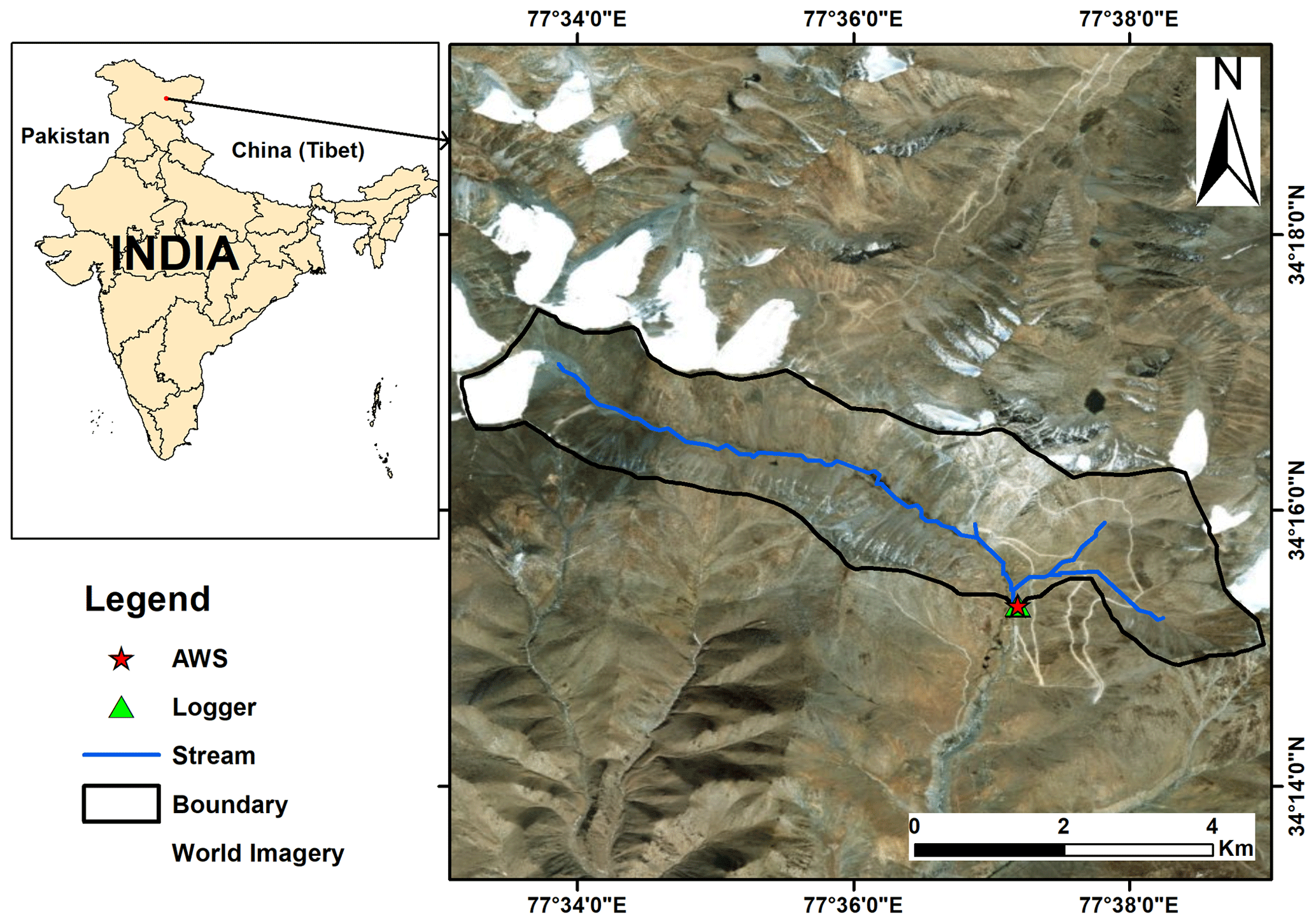
Figure 1 Location of the study site in the upper Ganglass catchment. (Base image sources for the right panel: © Esri, DigitalGlobe, GeoEye, Earthstar Geographic's, CNES/Airbus DS, USDA, USGS, AEX, Getmapping, Aerogrid, IGN, IGP, swisstopo and the GIS user community). Please note that the above figure contains disputed territories.

2 Study area and data

2.1 Study area

The present study is carried out at South Pullu (34.25^∘ N, 77.62^∘ E; 4727 m a.s.l.) in the upper Ganglass catchment (34.25 to 34.30^∘ N and 77.50 to 77.65^∘ E), Leh, Ladakh (Fig. 1). Ladakh is a union territory of India and has a unique climate, hydrology and landforms. Leh is the district headquarter where long-term climate data are available (Bhutiyani et al., 2007). Long-term mean precipitation of Leh (1980–2017, 3526 m a.s.l.) is 115 mm (Lone et al., 2019; Thayyen et al., 2013), and the daily minimum and maximum temperatures during the period (2010 to 2012) range between −23.4 and 33.8 ^∘C (Thayyen and Dimri, 2014). The spatial area of the catchment is 15.4 km² and extends from 4700 m to 5700 m a.s.l. A small cirque glacier called Phuche glacier with an area of 0.62 km² occupies the higher elevations of the catchment, where a single stream originates and flows through the valley of the catchment. This stream flows intermittently with a maximum mean daily flow of 3.57 m³ s⁻¹ (wet years) and 0.4 m³ s⁻¹ (dry years) from May to October.

The catchment is part of the main Indus River basin and belongs to the geological unit of the Ladakh batholith (Thakur, 1981). The study catchment also consists of steep mountain slopes with the valley bottom filled with glacio-fluvial deposits. Other sporadic landforms found in the catchment include patterned ground, boulder fields, peatlands, high-elevation wetlands and a small lake. Many of these landforms point towards intense frost action in the area.

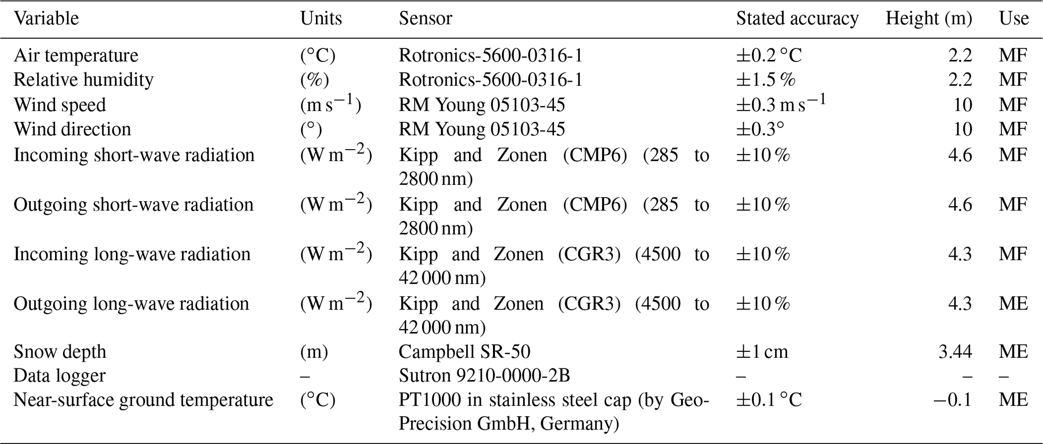
Table 1 Technical parameters of different sensors at South Pullu (4727 m a.s.l.) in the upper Ganglass catchment, Leh. (MF: model forcing, ME: model evaluation).

2.2 Meteorological data used

The automatic weather station (AWS) in the catchment is located at an elevation of 4727 m a.s.l. at South Pullu (Fig. 1). It is located in a wide south-east-oriented deglaciated valley. The site has a local slope angle of 15^∘, and the soil is sparsely vegetated. Weather data have been collected by a Sutron automatic weather station from 1 September 2015 to 31 August 2017. The study years 1 September 2015 to 31 August 2016 and 1 September 2016 to 31 August 2017 hereafter in the text will be designated as 2015–2016 and 2016–2017, respectively. The variables measured include air temperature, relative humidity, wind speed and direction, incoming and outgoing short-wave and long-wave radiation, and snow depth (Table 1). The snow depth is measured using a Campbell SR50 sonic ranging sensor with a nominal accuracy of ±1 cm (Table 1). To reduce the noise of the measured snow depth, a 6 h moving average is applied. Near-surface ground temperature (GST) is measured at a depth of 0.1 m near the AWS using a miniature temperature data logger (MTD) manufactured by GeoPrecision GmbH, Germany. GST data were available only from 1 September 2016 to 31 August 2017 and are used for model evaluation only. All the four solar radiation components, i.e. incoming short-wave (SW_in), outgoing short-wave (SW_out), incoming long-wave (LW_in) and outgoing long-wave (LW_out) radiation, were measured. Before using these data in the SEB calculations, necessary corrections were applied (Nicholson et al., 2013; Oerlemans and Klok, 2002): (a) all the values of SW_in<5 W m⁻² are set to zero, and (b) when SW_out>SW_in (3 % of data under study), it indicates that the upward-looking sensor was covered with snow (Oerlemans and Klok, 2002). The SW_out can be higher than SW_in at high-elevation sites such as this one due to high solar zenith angle during the morning and evening hours (Nicholson et al., 2013). In such cases, SW_in was corrected by SW_out divided by the accumulated albedo, calculated by the ratio of measured SW_out and measured SW_in for a 24 h period (van den Broeke et al., 2004).

3 Methods

3.1 Estimation of precipitation from snow height

In high-elevation and remote sites, the measurement of snowfall is a difficult task with an undercatch of 20 %–50 % (Rasmussen et al., 2012; Yang et al., 1999). At the South Pullu station, daily precipitation including snow was measured using a non-recording rain gauge. In this high-elevation area, an undercatch of 23 % of snowfall was reported earlier (Thayyen et al., 2015). In this study, the total precipitation was recorded at daily temporal resolution, whereas the other meteorological forcings including SR50 snow depth were recorded at hourly time steps. Therefore, to match the temporal resolution of precipitation data with the other meteorological forcing data, we adopted the method proposed by Mair et al. (2016), called Estimating SOlid and Liquid Precipitation (ESOLIP). This method makes use of snow depth and meteorological observations to estimate the sub-daily solid precipitation in terms of snow water equivalent (SWE). In ESOLIP, we considered daily liquid precipitation only. The ESOLIP method consists of the following steps:

1. Precipitation readings related to simplified relative humidity (RH) and global short-wave radiation criteria (e.g. RH >50 % and SW_in<400 W m⁻²) are filtered.

2. For precipitation type determination, wet bulb temperature (T_w) is used to differentiate between rain and snow, i.e. rainfall is assumed for T_w<1 (SWE estimation), and if T_w>=1 (rain), T_w is estimated by solving the psychrometric formula implicitly: $e=E\left(T_{\mathrm{w}}\right)-\mathit{\gamma }(T_{\mathrm{a}}-T_{\mathrm{w}}$), where T_a is the air temperature, e (hPa) is the vapour pressure in the air, E (hPa) is the saturation vapour pressure, and γ (hPa K⁻¹) is the psychrometric constant depending on air pressure.

3. For the estimation of density, the fresh snow density (ρ) is estimated based on air temperature (T_a) and wind speed measured at 10 m height (u₁₀) as follows (Jordan et al., 1999):

   $$\begin{array}{}\text{(1)}& \begin{array}{rl}\mathit{\rho }& =\mathrm{500}\cdot [\mathrm{1}-\mathrm{0.951}\cdot \exp (-\mathrm{1.4}\\ & \cdot (\mathrm{278.15}-T_{\mathrm{a}}{)}^{-\mathrm{1.15}}-\mathrm{0.008}{u}_{\mathrm{10}}^{\mathrm{1.7}})]\end{array}\end{array}$$

   for $\mathrm{260.15}<T_{\mathrm{a}}\le \mathrm{275.65}$ K.

   $$\begin{array}{}\text{(2)}& \mathit{\rho }=\mathrm{500}\cdot [\mathrm{1}-\mathrm{0.904}\cdot \exp (-\mathrm{0.008}{u}_{\mathrm{10}}^{\mathrm{1.7}}\left)\right]\end{array}$$

   for T_a≤260.15 K.

4. To estimate the SWE (SWE $=h\cdot \mathit{\rho }$) of single snowfall events using snow depth (h) measurements, an identification of the snow height increments of the single snowfall events and an accurate estimate of the snow density are necessary.

3.2 Modelling of surface energy balance

In this study, the open-source model GEOtop version 2.0 (hereafter GEOtop) (Endrizzi et al., 2014; Rigon et al., 2006) was used for the modelling of point surface energy balance, including the evolution of the snow depth and the transfer of heat and water in snow and soil. GEOtop represents the combined ground heat and water balance, as well as the exchange in energy with the atmosphere by taking into consideration the radiative and turbulent heat fluxes. The model has a multi-layer snowpack and solves the energy and water balance of the snow cover and soil including the highly non-linear interactions between the water and energy balance during soil freezing and thawing (Dall'Amico et al., 2011a). It can be applied in complex terrain which makes it possible to account for topographical and other environmental variability (Fiddes et al., 2015; Gubler et al., 2013).

Previous studies have successfully applied GEOtop in mountain regions e.g. simulating snow depth (Endrizzi et al., 2014), snow cover mapping (Dall'Amico et al., 2011b, 2018; Engel et al., 2017; Zanotti et al., 2004), ecohydrological processes (Bertoldi et al., 2010; Chiesa et al., 2014), modelling of ground temperatures in complex topography (Bertoldi et al., 2010; Endrizzi et al., 2014; Fiddes and Gruber, 2012; Gubler et al., 2013), water and energy fluxes (Hingerl et al., 2016; Rigon et al., 2006; Soltani et al., 2019), evapotranspiration (Mauder et al., 2018), and permafrost distribution (Fiddes et al., 2015).

Generally, the surface energy balance (SEB) (Eq. 3) is written as a combination of net radiation (R_n), sensible (H) and latent heat (LE) flux, heat conduction into the ground or to the snow (G), and it must balance at all times (Oke, 2002):

$$\begin{array}{}\text{(3)}& R_{\mathrm{n}}+H+\text{LE}+G-F_{\mathrm{surf}}=\mathrm{0},\end{array}$$

where F_surf is the resulting latent heat flux in the snowpack due to melting or freezing. We use the sign convention that energy fluxes towards the surface are positive and fluxes away from the surface are negative (Mölg, 2004). During the summertime, when conditions for snow melting are prevailing at the ground surface, F_surf is negative (loss from the system) as a result of energy available for melting snow and warming the ground under snow-free conditions. Positive F_surf (gain to the system) during summertime is the energy released to refreeze the water and represents the freezing flux.

In cold regions, the SEB is a complex function of solar radiation, seasonal snow cover, vegetation, near-surface moisture content and atmospheric temperature (Lunardini, 1981). Based on the available in situ data, the calculation of SEB components like H, LE and G is difficult. For example, in the calculation of turbulent heat fluxes (H and LE), the wind speed and temperature measurements near the ground surface are required at two heights, which are generally not available. Therefore, the parameterization method, like the bulk aerodynamic method, is used, which is valid under statically neutral conditions in the surface layer (Stull, 1988). Hence, the application of a tested model like GEOtop is a good alternative for the estimation of these fluxes. In GEOtop, the general SEB equation (Eq. 3) is linked with the water balance and is written as follows:

$$\begin{array}{}\text{(4)}& F_{\mathrm{surf}}\left(T_{\mathrm{s}}\right)={\text{SW}}_{\mathrm{n}}+{\text{LW}}_{\mathrm{n}}\left(T_{\mathrm{s}}\right)+H\left(T_{\mathrm{s}}\right)+\text{LE}\left(T_{\mathrm{s}},{\mathit{\theta }}_{\mathrm{w}}\right),\end{array}$$

where T_s, the temperature of the surface, is unknown, SW_n is the net short-wave radiation, LW_n is the net long-wave radiation, and F_surf is a function of T_s. Other terms in Eq. (4) which are a function of T_s include LW_n, H and LE. In addition, LE depends also on the soil moisture at the surface (θ_w), linking the SEB and water balance equations. The equations and the key elements of GEOtop are explained in Endrizzi et al. (2014); here, only a brief description of the equations that are of interest in this study is given. LW_out is estimated using the Stefan–Boltzmann law:

$$\begin{array}{}\text{(5)}& {\text{LW}}_{\mathrm{out}}={\in }_{\mathrm{s}}\mathit{\sigma }{T}_{\mathrm{s}}^{\mathrm{4}},\end{array}$$

where ∈_s is the surface emissivity, and σ is the Stefan–Boltzmann constant ($\mathrm{5.67}\times {\mathrm{10}}^{-\mathrm{8}}$ W m⁻² K⁻⁴).

The turbulent fluxes (H and LE) are driven by the gradients of temperature and specific humidity between the air and the surface and due to turbulence caused by winds as the primary transfer mechanism in the boundary layer (Endrizzi, 2007). GEOtop estimates the turbulent heat fluxes using the flux-gradient relationship (Brutsaert, 1975; Garratt, 1994) as follows:

$$\begin{array}{}\text{(6)}& {\displaystyle }H={\mathit{\rho }}_{\mathrm{a}}{c}_p{w}_{\mathrm{s}}{\displaystyle \frac{T_{\mathrm{a}}-T_{\mathrm{s}}}{r_{\mathrm{a}}}},\text{(7)}& {\displaystyle }\text{LE}={\mathit{\beta }}_{YP}{L}_{\mathrm{e}}{\mathit{\rho }}_{\mathrm{a}}{c}_p{w}_{\mathrm{s}}{\displaystyle \frac{Q_{\mathrm{a}}-{\mathit{\alpha }}_{YP}{Q}_{\mathrm{s}}^{\ast }}{r_{\mathrm{a}}}},\end{array}$$

where ρ_a is the air density (kg m⁻³), w_s is the wind speed (m s⁻¹), c_p the specific heat at constant pressure (J kg⁻¹ K⁻¹), L_e the specific heat of vaporization (J kg⁻¹), Q_a and $Q_{\mathrm{s}}^{\ast }$ are the specific humidity of the air (kg kg⁻¹) and saturated specific humidity at the surface (kg kg⁻¹), respectively, β_YP and α_YP are the coefficients that take into account the soil resistance to evaporation and only depend on the liquid water pressure close to the soil surface, and r_a is the aerodynamic resistance (–). The aerodynamic resistance is obtained by applying the Monin–Obukhov similarity theory (Monin and Obukhov, 1954), which requires that values of wind speed, air temperature and specific humidity are available at least at two different heights above the surface, but the values of these variables are generally measured at a standard height above the surface and can be used for the ground surface with the following assumptions: (a) the air temperature is equal to the ground surface temperature; however, this assumption leads to the boundary condition's non-linearity, (b) the specific humidity is equal to ${\mathit{\alpha }}_{YP}{Q}_{\mathrm{s}}^{\ast }$, and (c) wind speed is equal to zero.

The coefficients β_YP and α_YP (Eqs. 8 and 9) are calculated according to the parameterization of Ye and Pielke (1993) which considers evaporation as the sum of the proper evaporation from the surface and diffusion of water vapour in soil pores at greater depths:

$$\begin{array}{}\text{(8)}& {\displaystyle }{\mathit{\beta }}_{YP}={\mathit{\chi }}_{\mathrm{p}}\left(g\right)-{\displaystyle \frac{\left[{\mathit{\chi }}_{\mathrm{p}}\left(g\right)-{\mathit{\theta }}_{\mathrm{g}}\right]}{\mathrm{1}+\frac{{\mathit{\chi }}_{\mathrm{p}}\left(\mathrm{1}\right)-{\mathit{\theta }}_{\left(\mathrm{1}\right)}}{{\mathit{\chi }}_{\mathrm{p}}\left(g\right)-{\mathit{\theta }}_{\mathrm{g}}}\frac{r_{\mathrm{a}}}{r_{\mathrm{d}}}}},\text{(9)}& {\displaystyle }{\mathit{\alpha }}_{YP}={\displaystyle \frac{\mathrm{1}}{{\mathit{\beta }}_{YP}}}\left[{\mathit{\theta }}_{\mathrm{g}}+{\displaystyle \frac{{\mathit{\chi }}_{\mathrm{p}}\left(\mathrm{1}\right)-{\mathit{\theta }}_{\left(\mathrm{1}\right)}}{\mathrm{1}+\frac{{\mathit{\chi }}_{\mathrm{p}}\left(\mathrm{1}\right)-{\mathit{\theta }}_{\left(\mathrm{1}\right)}}{{\mathit{\chi }}_p\left(g\right)-{\mathit{\theta }}_{\mathrm{g}}}\frac{r_{\mathrm{a}}}{r_{\mathrm{d}}}}}{\displaystyle \frac{r_{\mathrm{a}}}{r_{\mathrm{d}}}}{h}_{\mathrm{s}\left({\mathit{\theta }}_{\mathrm{1}}\right)}{\displaystyle \frac{q_{\left(\mathrm{Ts}\mathrm{1}\right)}^{\mathrm{sat}}}{q_{\left(\mathrm{Tg}\right)}^{\mathrm{sat}}}}\right],\end{array}$$

where q^sat is the specific humidity in saturated condition, the subscripts “g” and 1 refer to the ground surface and a thin layer next to the ground surface, respectively, θ is the volumetric water content of the soil, χ_p is the volumetric fraction of soil pores, h_s is the relative humidity in the pores, T_g is the temperature at the ground surface, and r_d is the soil resistance to water vapour diffusion.

3.2.1 The heat equation and snow depth

Equation (10) represents the energy balance in a soil volume subject to phase change in GEOtop (Endrizzi et al., 2014):

$$\begin{array}{}\text{(10)}& {\displaystyle \frac{\partial U^{\mathrm{ph}}}{\partial t}}+\mathrm{\nabla }\mathbf{G}+S_{\mathrm{en}}-{\mathit{\rho }}_{\mathrm{w}}\left[L_{\mathrm{f}}+c_{\mathrm{w}}\left(T-T_{\mathrm{ref}}\right)\right]S_{\mathrm{w}}=\mathrm{0},\end{array}$$

where U^ph is the volumetric internal energy of soil (J m⁻³) subject to phase change, t(s) is time, G is the heat conduction flux (W m⁻²), S_en is the energy sink term (W m⁻³), S_w is the mass sink term (s⁻¹), L_f (J kg⁻¹) is the latent heat of fusion, ρ_w is the density of liquid water in soil (kg m⁻³), c_w is the specific thermal capacity of water (J kg⁻¹ K⁻¹), T (^∘C) is the soil temperature, and T_ref (^∘C) is the reference temperature at which the internal energy is calculated. If G is written according to Fourier's law, Eq. (10) becomes

$$\begin{array}{}\text{(11)}& {\displaystyle \frac{\partial U^{\mathrm{ph}}}{\partial t}}+\mathrm{\nabla }\left({\mathit{\lambda }}_{\mathrm{T}}\mathrm{\nabla }T\right)+S_{\mathrm{en}}-{\mathit{\rho }}_{\mathrm{w}}\left[L_{\mathrm{f}}+c_{\mathrm{w}}\left(T-T_{\mathrm{ref}}\right)\right]S_{\mathrm{w}}=\mathrm{0},\end{array}$$

where λ_T is the thermal conductivity (W m⁻¹ K⁻¹), which is a non-linear function of temperature because the proportion of liquid water and ice contents depends on temperature. For the calculation of λ_T, GEOtop uses the method proposed by Cosenza et al. (2003). A detailed description of the heat conduction equation used in GEOtop can be found in Endrizzi et al. (2014).

The snow cover buffers the energy exchange between the soil and atmosphere and critically influences the soil thermal regime. GEOtop includes a multi-layer, energy-based, Eulerian snow modelling approach with similar equations to the ones used for the soil matrix (Endrizzi et al., 2014). The discretization of snow in GEOtop is carried out in such a way that the thermal gradients inside the snowpack are described accurately. The effective thermal conductivity at the interface between snow and ground is calculated similarly as between different soil layers using the method of Cosenza et al. (2003). Fresh snow density is computed using the Jordan et al. (1999) formula, which is based on air temperature and wind speed. More details about the snow metamorphism compaction rates and the snow discretization in GEOtop can be found in Appendix D2 and D3 of Endrizzi et al. (2014).

3.2.2 Model setup and forcings

The 1D GEOtop simulation was carried out at South Pullu (Fig. 1). The soil column is 10 m deep and is discretized into 19 layers, with thickness increasing from the surface to the deeper layers. The top eight layers close to the ground surface were resolved with thicknesses ranging from 0.1 to 1 m because of the higher temperature and water pressure gradients near the surface, while the lowest layer is 4.0 m thick. The snowpack is discretized in 10 layers which are finer at the interfaces with the atmosphere and soil.

The model was initialized with a uniform soil temperature of −0.5 ^∘C and spun up by repeatedly modelling the soil temperature down to 1 m (2 years ⋅ 25 times) and then using the modelled soil temperatures as an initial condition to repeatedly simulate soil temperature down to 10 m (2 years ⋅ 25 times) (cf., Fiddes et al., 2015; Gubler et al., 2013; Pogliotti, 2011). Prior tests showed that the minimum number of repetitions required to bring the soil column to equilibrium was 25 (Fig. S1). The values of all the input parameters used in the study are given in Tables A1 to A4 in the Supplement.

The input meteorological data required for running the 1D GEOtop model include time series of precipitation, air temperature, relative humidity, wind speed, wind direction (WD) and solar radiation components and the description of the site (slope angle, elevation, aspect and sky view factor) for the simulation point. The model was run at an hourly time step corresponding to the measurement time step of the meteorological data.

3.2.3 Model performance evaluation

While the accuracy of simulated energy fluxes cannot be quantified, the quality of GEOtop simulations is evaluated based on snow depth, GST and LW_out. These variables were chosen because they have not been used to drive the model, and they represent different physical processes affected by surface energy balance. The melt-out date of the snow depth is hereby a good indicator showing how good the surface mass and energy balance is simulated, whereas GST is the result of all the processes occurring at the ground surface such as radiation, turbulence, and latent and sensible heat fluxes (Gubler, 2013). LW_out is governed by the temperature and emissivity at the surface, and Eq. (3) is solved in terms of the surface temperature. Therefore, LW_out is used as a proxy for the evaluation of the SEB.

Model performance is evaluated based on the measured and the simulated time series. Typically, a variety of statistical measures are used to assess the model performance because no single measure encapsulates all aspects of interest. In this study, R², mean bias difference (MBD) and the root mean square difference (RMSD), mean bias (MB) and root mean square error (RMSE), and Nash–Sutcliffe efficiency coefficient (NSE; Nash and Sutcliffe, 1970) were used (Eqs. S1 to S6).

4 Results

4.1 Model evaluation

In this section, the capability of GEOtop to reproduce snow depth, GST and LW_out based on standard model parameters obtained from the literature (Tables 2 and 3; Gubler et al., 2013) was evaluated, i.e. model results were not improved by trial and error.

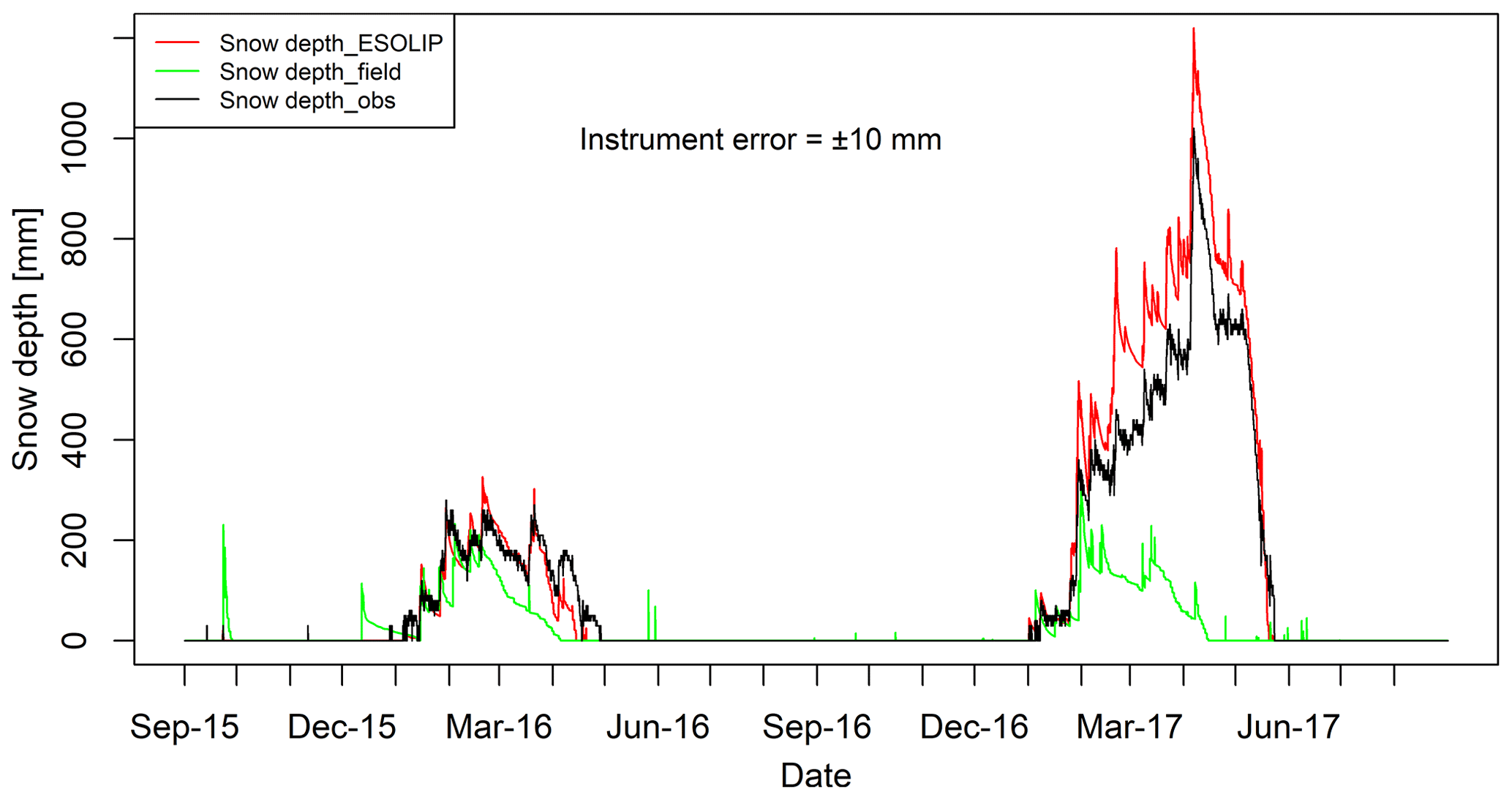
Figure 2 Comparison of hourly observed and GEOtop-simulated snow depth at South Pullu (4727 m a.s.l.) from 1 September 2015 to 31 August 2017. The black line denotes the snow depth measured in the field by the SR50 sensor. The red (Snow depth_ESOLIP) and green (Snow depth_field) lines in the plot indicate the GEOtop-simulated snow depth based on ESOLIP-estimated precipitation and precipitation measured in the field, respectively.

4.1.1 Evaluation of snowpack

Snow depth variations simulated by GEOtop are compared with observations from 1 September 2015 to 31 August 2017 (Fig. 2). The model captures the peaks and start and melt-out dates of the snowpack, as well as overall fluctuations (Fig. S2; R²=0.98, RMSE = 59.5 mm, MB = 16.7 mm, NSE = 0.91, instrument error $=\pm \mathrm{10}$ mm). The maximum simulated snow height (h) was 1219 mm in comparison to the 1020 mm measured in the field. In the low snow year (2015–2016), the maximum simulated h was 326 mm in comparison to 280 mm measured in the field. During the melting period of the low and high snow years, the snow depth was slightly underestimated. However, during the accumulation period of high snow year (2016–2017), h was rather overestimated by the model.

The performance of the ESOLIP-estimated precipitation was evaluated against a control run with precipitation data measured in the field (Fig. 2). ESOLIP is the superior approach for precipitation estimation when snow depth and necessary meteorological measurements are available.

Figure 2 shows the comparison of hourly observed and GEOtop-simulated snow depth at South Pullu (4727 m a.s.l.) from 1 September 2015 to 31 August 2017. The black line denotes the snow depth measured in the field by the SR50 sensor. The red (Snow depth_ESOLIP) and green (Snow depth_field) lines in the plot indicate the GEOtop-simulated snow depth based on ESOLIP-estimated precipitation and precipitation measured in the field, respectively.

Figure 3 Comparison of daily mean observed (GST_obs; ^∘C) and GEOtop-simulated near-surface ground temperature (GST_sim; ^∘C) at South Pullu (4727 m a.s.l.) from 1 September 2016 to 31 August 2017.

4.1.2 Evaluation of near-surface ground temperatures (GST)

GST is simulated (GST_sim) on an hourly basis and compared with the observed values (GST_obs) near the AWS, available from 1 September 2016 to 31 August 2017 (Fig. 3). The results show a reasonably good linear agreement between the simulated and observed GSTs (Fig. S3; R²=0.97, MB $=-\mathrm{0.11}$ ^∘C, RMSE = 1.63 ^∘C, NSE = 0.95, instrument error $=\pm \mathrm{0.1}$^∘). The model estimated the dampening of soil temperature fluctuations by the snowpack and the zero-curtain period at the end of the melt-out of the snowpack reasonably well.

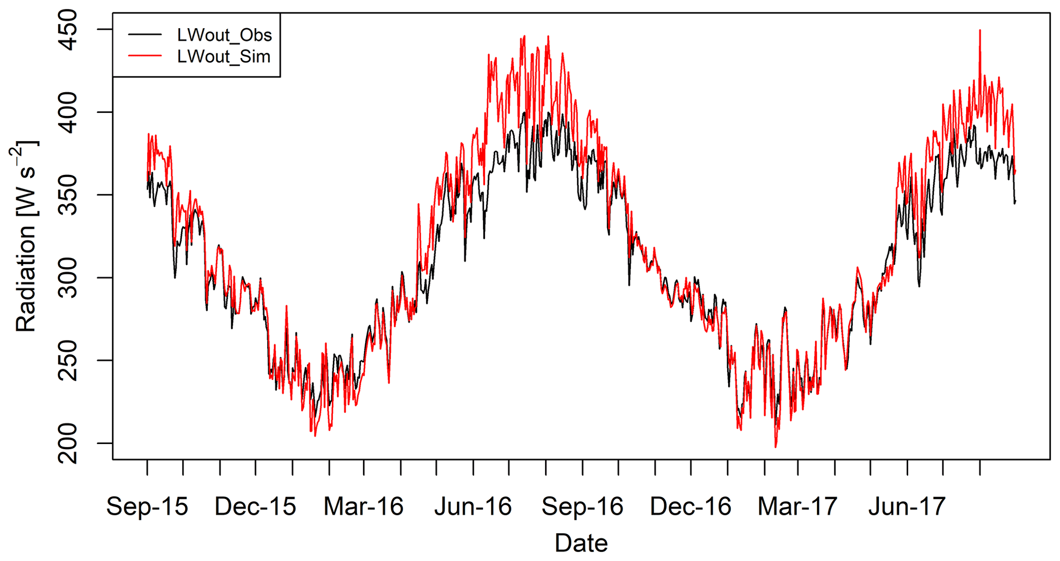
Figure 4 Comparison of daily mean observed (LW_out_obs) and GEOtop-simulated (LW_out_sim) outgoing long-wave radiation at South Pullu (4727 m a.s.l.) from 1 September 2015 to 31 August 2017. The instrument error for the Kipp and Zonen (CGR3) (4500 to 42 000 nm) radiometer is ±10 %.

4.1.3 Evaluation of outgoing long-wave radiation

Modelled LW_out is evaluated with the observed measurements, and a comparison of daily mean observed and simulated LW_out is shown in Fig. 4. The daily mean LW_out matches very well with the observed data except during summer months when the simulated LW_out was slightly overestimated compared to the observed values. The hourly LW_out shows a good linear relationship (Fig. S4; R²=0.93, NSE = 0.73), but the GEOtop slightly overestimates the LW_out (MBD = 3 %) with an RMSD value of 10 % (instrument error $=\pm \mathrm{10}$ %).

Based on the evaluation of LW_out, the GEOtop can simulate the surface temperature at the point scale; therefore, we believe that it can reasonably calculate the different SEB components.

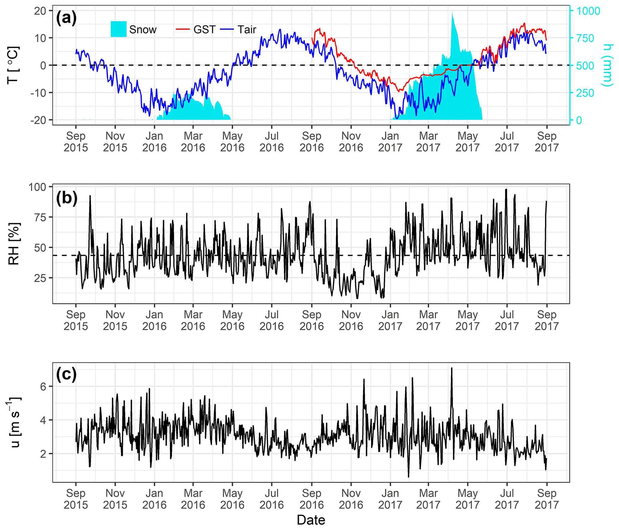
Figure 5 Daily mean values of observed (a) air temperature (blue) and 1-year GST (red) (T; ^∘C) with snow depth (mm) on the secondary axis, (b) relative humidity (RH; %) with a dashed line as mean RH, and (c) wind speed (u; m s⁻¹) at South Pullu (4727 m a.s.l.) in the upper Ganglass catchment, Leh, from 1 September 2015 to 31 August 2017.

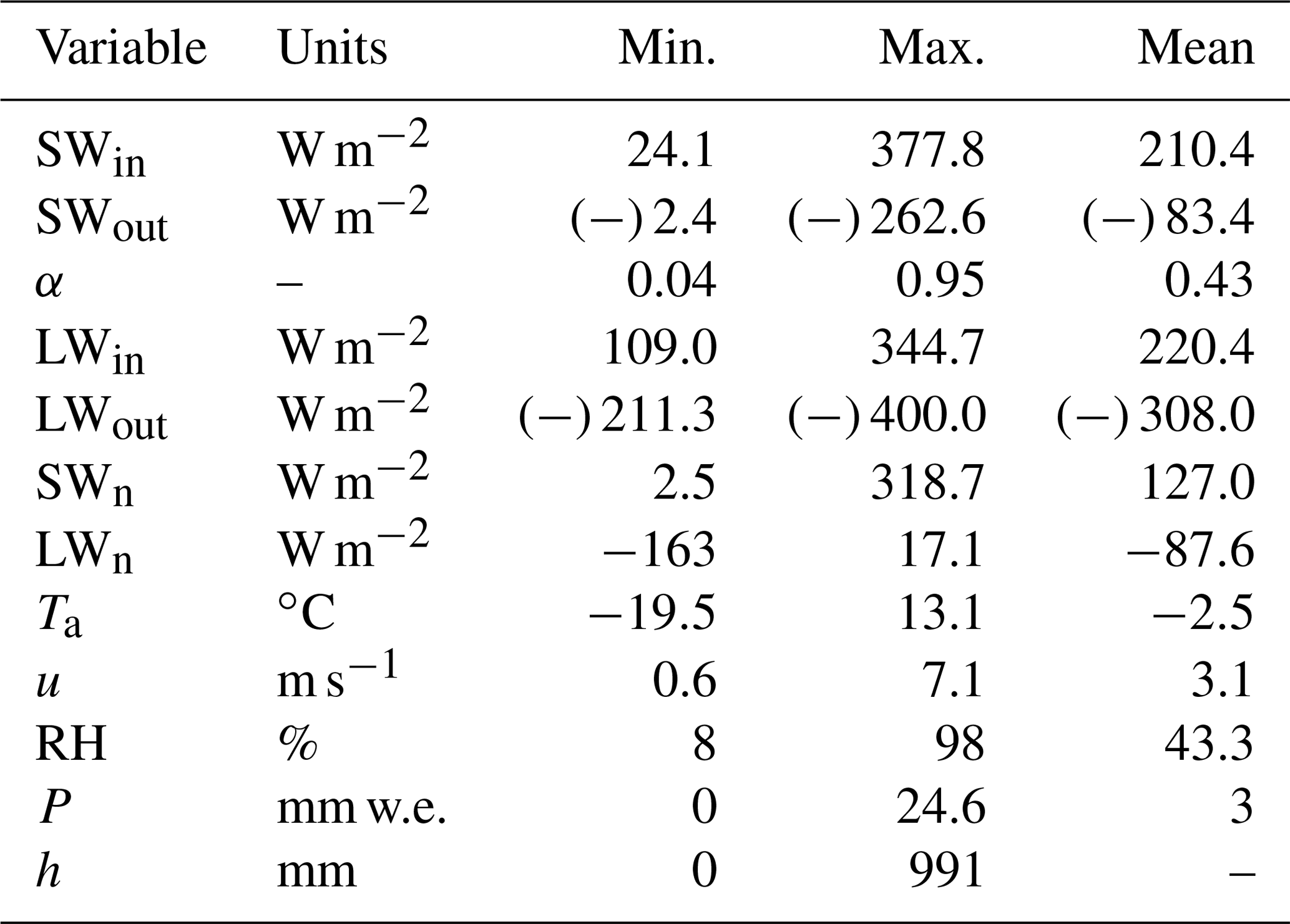
Table 2 Range of observed daily mean radiation components (SW_in, SW_out, LW_in and LW_out, SW_n, LW_n), surface albedo (α), net short-wave and long-wave radiation (SW_n and LW_n), air temperature (T_a), wind speed (u), relative humidity (RH), precipitation (P), and snow depth (h) for the study period (1 September 2015 to 31 August 2017) at South Pullu (4727 m a.s.l.).

4.2 Meteorological characteristics

The range of the meteorological variables measured at the South Pullu (4727 m a.s.l.) study site is given in Table 2 to provide an overview of the prevailing weather conditions in the study region. The daily mean air temperature (T_a) throughout the study period varies between −19.5 and 13.1 ^∘C with a mean annual average temperature (MAAT) of −2.5 ^∘C (Fig. 5a). T_a shows significant seasonal variations, and measured hourly temperatures at the study site range between −23.7 ^∘C in January and 18.1 ^∘C in July. During the 2-year study period, sub-zero mean monthly temperature prevailed for 7 months from October to April in both years. The mean monthly T_a during pre-winter months (September to December) of 2015–2016 and 2016–2017 was −4.6 and −2.7 ^∘C, respectively. During the core winter months (January to February) of 2015–2016 and 2016–2017, the respective mean monthly T_a was −13.1 and −13.7 ^∘C, and, for post-winter months (March and April), mean monthly T_a was −5.8 and −8 ^∘C, respectively. For summer months (May to August), the respective mean monthly T_a was 6.6 and 5.5 ^∘C. A sudden change in the mean monthly T_a characterizes the onset of a new season, and the most evident inter-season change was found between the winter and summer with a difference of about 16 ^∘C for both years.

The mean daily GST recorded by the logger near the AWS (1 September 2016 to 31 August 2017) is plotted along with air temperature (Fig. 5a). The mean daily GST ranges from −9.7 to 15.4 ^∘C with a mean annual GST of 2.1 ^∘C. The GST followed the pattern of air temperature but damped during winter due to the insulating effect of the snow cover. GST was generally higher than T_a except for a short period during snowmelt. The snow depth shown in Fig. 5a is further described in Sect. 4.3.

Mean relative humidity (RH) was equal to 43 % during the study period (Fig. 5b). The daily average wind speed (u) ranges between 0.6 (29 January 2017) and 7.1 m s⁻¹ (6 April 2017) with a mean wind speed of 3.1 m s⁻¹ (Fig. 5c). The instantaneous hourly u was plotted as a function of wind direction (WD) (Fig. S5) for the study period and showed a persistent dominance of katabatic and anabatic winds at the study site, which is typical of a mountain environment. The daily average WD during the study period was south-east (148^∘).

The daily measured annual total precipitation at the study site equals 97.8 and 153.4 mm w.e. during the years 2015–2016 and 2016–2017, respectively. After adding 23 % undercatch (Thayyen et al., 2015) to the total snow measurements, the total precipitation amount equals 120.3 and 190.6 mm w.e. for the years 2015–2016 and 2016–2017, respectively. During the study period, the observed highest single-day precipitation was 20 mm w.e. recorded on 23 September 2015, and the total number of precipitation days was limited to 63. The snowfall occurs mostly during the winter period (December to March), with some years witnessing extended intermittent snowfall till mid-June, as experienced in this study during the year 2016–2017.

The precipitation estimated by the ESOLIP approach at the study site equals 92.2 and 292.5 mm w.e. during the years 2015–2016 and 2016–2017, respectively. The comparison between observed precipitation (mm w.e.) and the one estimated by the ESOLIP approach is given in (Table S1). In Table S1, the difference between the observed precipitation (mm w.e.) and the one estimated by the ESOLIP approach is mainly due to the undercatch of winter snow recorded by the ordinary rain gauge.

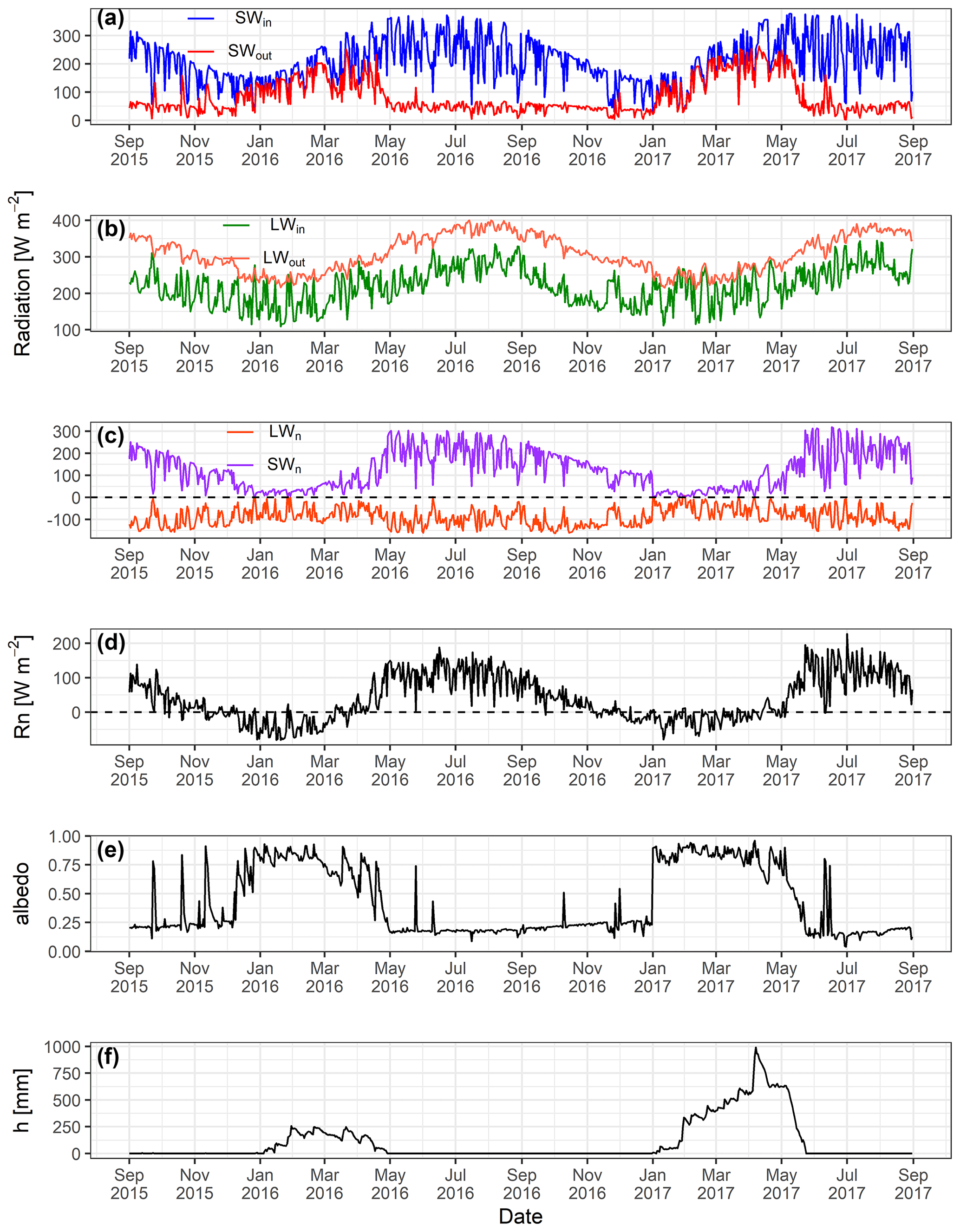
Figure 6 Observed daily mean values of (a) incoming (SW_in) and outgoing (SW_out) short-wave radiation, (b) incoming (LW_in) and outgoing long-wave (LW_out) radiation, (c) net short-wave (SW_n) and long-wave radiation (LW_n), and (d) net radiation (R_n), (e) surface albedo and (f) snow depth (h, mm) at South Pullu (4727 m a.s.l.) from 1 September 2015 to 31 August 2017.

4.3 Observed radiation components and snow depth

The observed daily mean variability in different components of radiation, albedo and snow depth from 1 September 2015 to 31 August 2017 at South Pullu (4727 m a.s.l.) is shown in Fig. 6. Daily mean SW_in varies between 24 and 378 W m⁻² (Table 2). Highest hourly instantaneous short-wave radiation recorded during the study period was 1358 W m⁻². Such high values of SW_in are typical of a high-elevation arid catchment (e.g. MacDonell et al., 2013). Persistent snow cover during the peak winter period for both years extending from January to March resulted in a strong reflection of SW_in radiation (Fig. 6a). During most of the non-snow period, mean daily SW_out radiation (Fig. 6a) remains more or less stable. The daily mean LW_in shows high variations (Fig. 3b, Table 2), whereas LW_out was relatively stable (Fig. 6b, Table 2). LW_out shows higher daily fluctuations during the summer months compared to the core winter months. SW_n follows the pattern of SW_in, and for both the years, during the wintertime, the SW_n was close to zero due to the high reflectivity of snow (Fig. 3c). LW_n values do not show any seasonality and remain more or less constant with a mean value of −88 W m⁻² (Fig. 6c).

Mean daily observed R_n values range from −80.5 to 227.1 W m⁻² with a mean value of 39.4 W m⁻² (Table 2). During both years, R_n was high in summer and autumn but low in winter and spring. From January to early April (2015–2016) and January to early May (2016–2017), when the surface was covered with seasonal snow, R_n rapidly declined to low values or even became negative (Fig. 6d). Daily mean observed albedo (α) at the study site ranges from 0.04 to 0.95 with a mean value of 0.43 (Fig. 6e, Table 2). However, the value of broadband albedo is not greater than 0.85 (Roesch et al., 2002), and the maximum value (0.95) recorded at the study site might be due to the instrumental error.

Both years experienced contrasting snow cover characteristics during the study period (Fig. 6f). The year 2015–2016 experienced shallow snow heights compared to 2016–2017. During 2015–2016, the snowpack had a maximum depth of 258 mm on 30 January 2016 compared to 991 mm on 7 April 2017. Snow cover duration was 120 d during 2015–2016 and 142 d during 2016–2017. The site became snow-free on 27 April 2016 and on 23 May 2017. Higher elevations of the catchment became snow-free around 15 July 2016, while the snow cover at glacier elevations persisted till 22 August 2017. In both years, the snow cover at lower elevations started to build up by the end of December, while the catchment had experienced sub-zero mean monthly temperatures already since October.

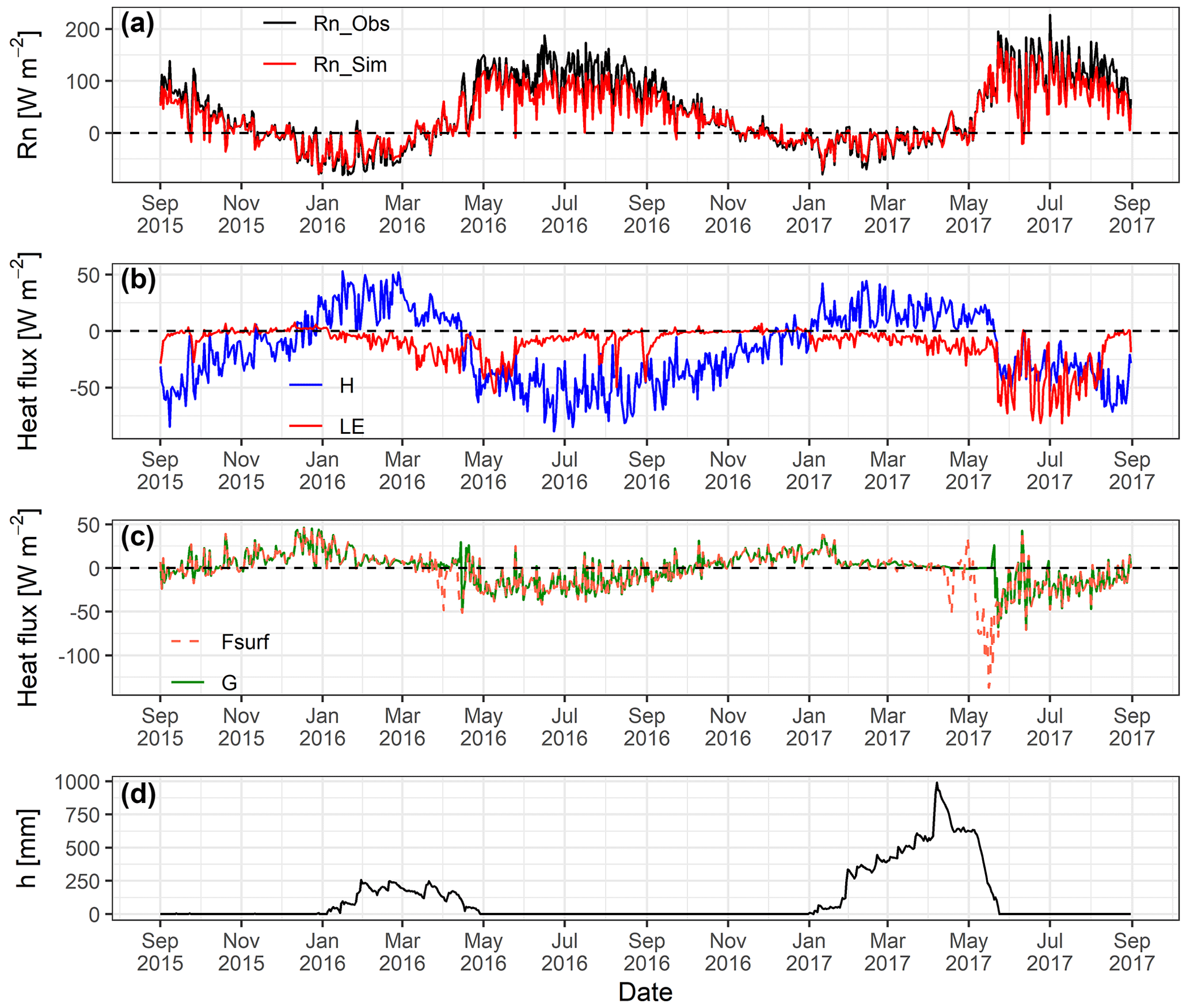
Figure 7 GEOtop-simulated daily mean values of surface energy balance components (a) observed and simulated net radiation (R_n), (b) sensible (H) and latent (LE) heat flux, (c) ground heat flux (G) and surface heat flux (F_surf), and (d) snow depth (h) at South Pullu (4727 m a.s.l.) from 1 September 2015 to 31 August 2017.

4.4 Modelled surface energy balance

The mean daily variability in SEB components is shown in Fig. 7. Simulated mean daily R_n values range between −78.9 and 175.6 W m⁻² with a mean value of 29.7 W m⁻². R_n shows the seasonal variability and decreases as the ground surface gets covered by seasonal snow cover during wintertime and increases as the ground surface become snow-free (Fig. 7a). The simulated R_n matches the observed R_n (Fig. 7a), which shows that the LW_out was estimated very well by the model. The daily mean sensible heat flux (H) ranges between −88.6 and 53 W m⁻² with a mean value of −15.6 W m⁻². H is positive from January to April (2015–2016) and January to June (2016–2017) due to the presence of seasonal snow cover (Fig. 7b). During the rest of the period, H remains negative and larger (∼35 W m⁻²) for most of the time. The seasonal variation in H points to a larger temperature gradient in summer than in winter. The daily mean latent heat flux (LE) ranges between −81.4 and 7.6 W m⁻² with a mean value of −11.2 W m⁻². During the snow-free freezing period (October to December) in both years, LE increases (from negative to zero) due to the freezing of soil moisture and fluctuates close to zero. When the surface is covered by snow, the LE is negative, indicating sublimation, and keeps increasing (more negative) after snowmelt indicating evaporation.

Table 3 Mean daily range of GEOtop-simulated SEB (W m⁻²) components for the study period (1 September 2015 to 31 August 2017) at South Pullu (4727 m a.s.l.).

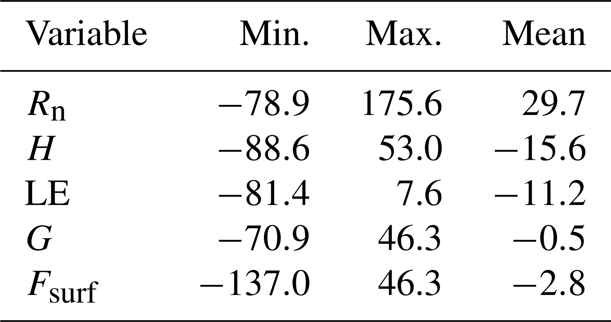
The heat conduction into the ground G is a comparatively small component in the SEB (Fig. 7c). Mean daily G values range between −70.9 and 46.3 W m⁻² with a mean value of −0.5 W m⁻². The sign of G, which shifts from negative during summer to positive during winter, is a function of the annual energy cycle. The heat flux available at the surface for melting (F_surf) ranges between −137 and 46.3 W m⁻² with a mean value of −2.8 W m⁻² (Table 3). During summer, when snowmelt conditions were prevailing, F_surf turns negative as a result of energy available for melt (Fig. 7c). The positive F_surf during summertime (when melting conditions are prevailing at the surface) is the energy used to refreeze the meltwater and represents the freezing heat flux.

The seasonal response of the diurnal variation in modelled SEB components (R_n, LE, H and G) for both years is shown in Figs. S6 and S7, respectively, and is described in detail in the Supplement. The main difference in diurnal changes was found during the winter and post-winter season of 2016–2017 because of the extended snow cover and is discussed in detail in Sect. 5.1.

During the study period, the proportional contribution of all SEB components shows that the net radiation component dominates (80 %), followed by H (9 %) and LE fluxes (5 %). The ground heat flux (G) was limited to 5 % of the total flux, and 1 % was used for melting the seasonal snow. The proportional contribution of each flux was calculated by following the approach of Zhang et al. (2013). The mean monthly modelled SEB components for both years are given in Table S2.

Furthermore, the partitioning of the energy balance shows that 52 % (−15.6 W m⁻²) of R_n (29.7 W m⁻²) was converted into H, 38 % (−11.2 W m⁻²) into LE, 1 % (−0.5 W m⁻²) into G and 9 % (−2.8 W m⁻²) for melting of seasonal snow. The partitioning was calculated by taking the mean annual average of each of the individual SEB components (LE, H and G) and then dividing these respective averages by the mean annual average of R_n. However, a distinct variation in energy flux is observed during the months of May–June of 2016–2017 due to the long-lasting snow cover.

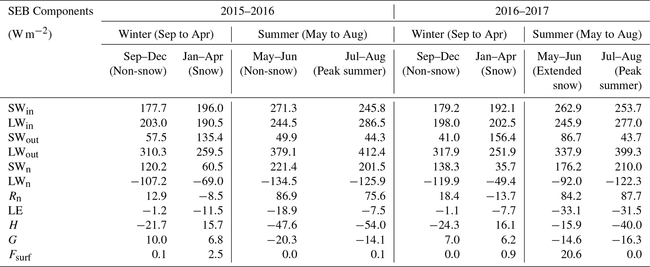
Table 4 Mean seasonal values of observed radiation and modelled surface energy balance components.

4.5 Comparison of seasonal variation in SEB during low and high snow years

The seasonal variation in observed radiation (SW_in, LW_in, SW_out, LW_out, SW_n, LW_n) and modelled SEB components (R_n, LE, H, G and F_surf) for the low and high snow years of the study period is analysed (Table 4). In addition to winter and summer, these seasons were further divided into two sub-seasons, i.e. early winter (September, October, November and December) and peak winter with snow (January, February, March and April). Similarly, the summer season was divided into early summer (May and June; some years with extended snow) and peak summer (July and August).

The mean seasonal SW_in was comparable in all seasons, whereas SW_out was significantly higher (86.7 W m⁻²) during the early summer season of 2016–2017 due to the extended snow cover compared to the preceding low snow year (49.9 W m⁻²). Similarly, LW_in shows similar seasonal values during the observation period, whereas LW_out shows a major difference during the early summer season with extended snow in 2016–2017 with reduced LW_out (337.9 W m⁻²) compared to the corresponding period in 2015–2016 (379.1 W m⁻²).

In both years, comparable SW_n values during the early winter period were observed. However, during the peak snow season of 2016–2017, SW_n was smaller (35.7 W m⁻²) compared to 2015–2016 (60.5 W m⁻²). Similarly, comparable SW_n during the peak summer season of both years is contrasted by lower SW_n (176.2 W m⁻²) in the early summer period of 2017 compared to 221.4 W m⁻² in 2016 on account of extended snow cover. The same trend is seen for LW_n as well with a lower value (−92 W m⁻²) in 2017 compared to 2016 (−134.5 W m⁻²). Seasonal variations in R_n followed the pattern of SW_n. The most significant difference of R_n is observed during early summer (May–June) and peak summer (July–August) of 2016 and 2017, respectively.

In both years, a comparable LE flux during the winter season is observed. A key difference is seen during the peak summer sub-season of 2016–2017, when LE was higher (−31.5 W m⁻²) compared to the 2015–2016 (−7.5 W m⁻²). The reason behind this is due to the reduced soil water content availability for evaporation during 2015–2016 in comparison to the high snow year 2016–2017. The comparatively large LE values during the snow sub-season in both years show that sublimation is a key factor in the region. The H was similar during the winter season in both years. The critical difference in H was observed during the extended snow sub-season of 2016–2017 when H was much smaller (−15.9 W m⁻²) compared to 2015–2016 (−47.6 W m⁻²) owing to the extended snow cover in 2016–2017.

Mean seasonal F_surf values were almost equal to zero during all seasons except during the snow sub-season of both years and extended snow sub-season of 2016–2017, when F_surf (heat flux available for melt) was much higher (20.6 W m⁻²) than during 2015–2016. From this inter-year seasonal comparison, it was found that the extended snow sub-season of 2016–2017 (high snow year) forced significant differences in energy fluxes between the years.

5 Discussion

5.1 SEB variations during low and high snow years

The realistic reproduction of seasonal and inter-annual variations in snow depth during the low (2015–2016) and high snow (2016–2017) years indicate a credible simulation of the SEB during the study period. We further investigated the response of SEB components during these years with contrasting snow cover for a better understanding of the critical periods of meteorological forcing and its characteristics.

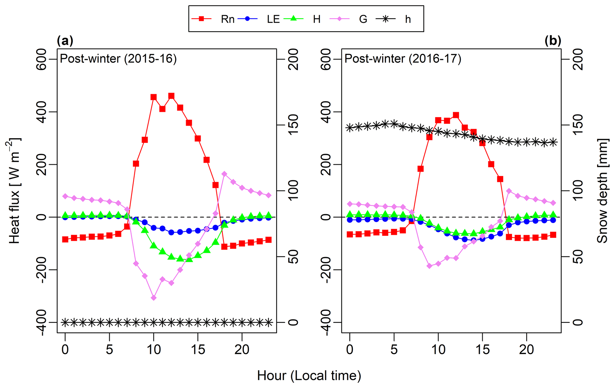
Figure 8 The diurnal change in GEOtop-modelled seasonal surface energy fluxes for (a) early summer 2015–2016 and (b) early summer 2016–2017 at South Pullu (4727 m a.s.l.), in the upper Ganglass catchment, Leh. The seasonal snow depth is plotted on the secondary axis.

To analyse this in more detail, we will discuss the diurnal variation in modelled SEB during the critical season, i.e. early summer, which showed significant differences in the amplitude of the energy fluxes (Fig. 8). During the early winter, peak winter and peak summer seasons (Figs. S6, S7), the diurnal variations of the SEB fluxes for the 2015–2016 year were more or less similar in comparison to the 2016–2017 year. However, during the early summer season of both years (Fig. 8), the SEB fluxes show different diurnal characteristics. In 2016–2017, the diurnal amplitude of R_n was slightly larger, whereas all other components (LE, H and G) were of almost zero amplitude (Fig. 8b). The smaller amplitude of LE, H and G is due to the smaller input (solar radiation) and the extended seasonal snow on the ground.

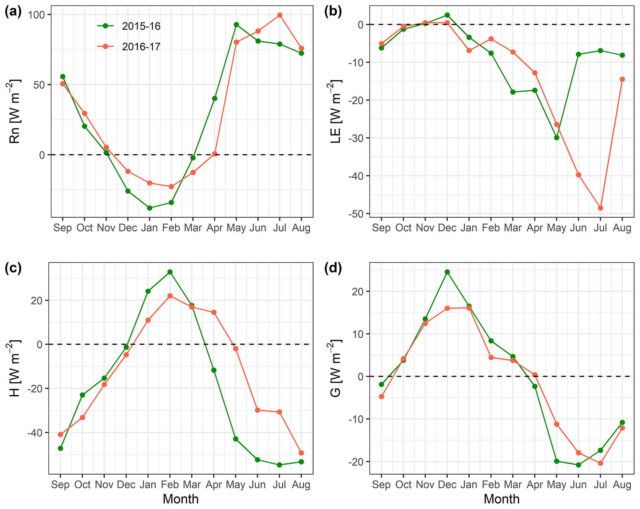
Figure 9 Comparison of estimated mean monthly surface energy balance components (W m⁻²) (a) R_n, (b) LE, (c) H and (d) G for the low (2015–2016) and high (2016–2017) snow years, at South Pullu (4727 m a.s.l.).

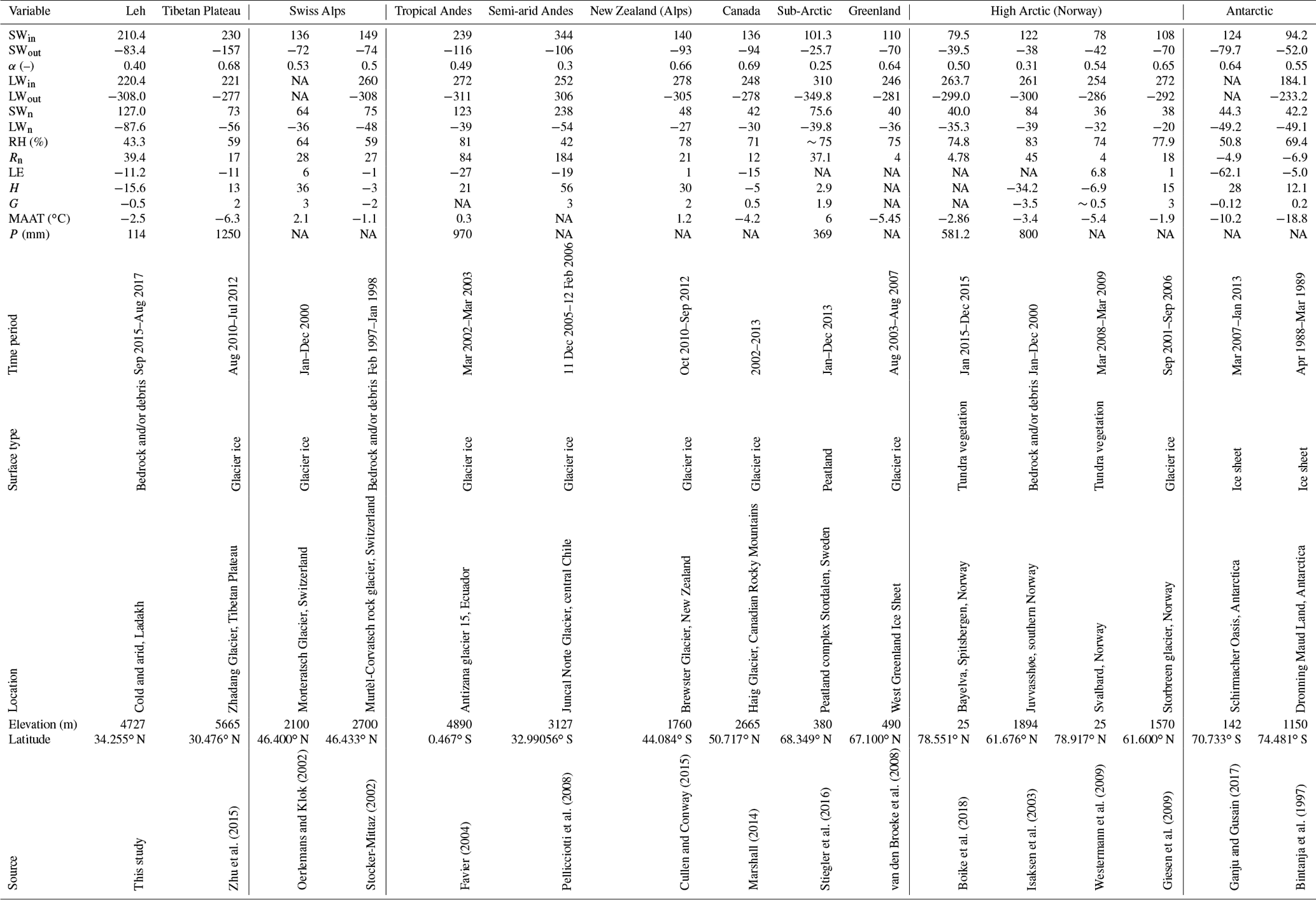
Table 5 Comparison of mean annual observed radiation and estimated SEB components and meteorological variables for different regions of the world. (SW_in: incoming short-wave radiation, SW_out: outgoing short-wave radiation, α: albedo, LW_in: incoming long-wave radiation, LW_out: outgoing long-wave radiation, SW_n: net short-wave radiation, LW_n: net long-wave radiation, RH: relative humidity, R_n: net radiation, LE: latent heat flux, H: sensible heat flux, G: ground heat flux, SEB: energy available at surface, MAAT: mean annual air temperature, P: precipitation, NA: not available). LE, H and G are modelled values. All the radiation components and heat fluxes are in units of watts per square metre (W m⁻²).

5.2 Impact of freezing and thawing process on surface energy fluxes

To understand the impact of freeze–thaw processes on surface energy fluxes, the variability in SEB components is shown in Fig. 9. The aim is to highlight the measurements of the study site as an example for SEB processes over seasonal frozen ground and permafrost in the cold and arid Indian Himalayan Region.

The freeze and thaw processes in the ground are complex and involve several physical and chemical changes, which include energy exchange, phase change, etc. (Chen et al., 2014; Hu et al., 2019). These processes amplify the interaction of fluxes between soil and atmosphere (Chen et al., 2014). In addition to the effect of seasonal snow, the R_n can also get affected by the seasonal freeze–thaw process of the ground. For example, when the seasonal frozen ground or permafrost begins to thaw in summer, R_n (Fig. 9a) increases due to the lower albedo of water than ice (Yao et al., 2020), and the opposite pattern happens during the freezing season. In Fig. 9d, during the seasonal freezing phase from September to December, the simulated mean monthly G starts to decrease and begins to change the sign from negative to positive due to the change in flux direction from soil to the atmosphere. However, during summer, the permafrost and seasonally frozen soil act as a heat sink because the thawing processes require a considerable amount of heat that is absorbed from the atmosphere by the soil (Eugster et al., 2000; Gu et al., 2015). In Fig. 9d, during the thawing phase from April to July, the simulated mean monthly G starts to increase and change sign due to the transfer of flux direction from the atmosphere to the soil. This pattern is consistent with the results from other studies on permafrost areas from the Tibetan Plateau (Chen et al., 2014; Hu et al., 2019; Zhao et al., 2000). In both low and high snow years (Fig. 9b and c), the mean monthly estimated H and LE heat fluxes show prominent seasonal characteristics, such as that the latent heat flux was highest in summer and lowest in winter. In contrast, the sensible heat flux was highest in early summer and gradually decreased towards the pre-winter season. A similar kind of variability in the LE and H is also reported from the seasonally frozen ground and permafrost regions of the Tibetan Plateau (Gu et al., 2015; Yao et al., 2011, 2020).

During the peak summer months (June to August, Fig. 9c), H tends to decrease or became relatively stable. This is primarily due to the thawing in the seasonally frozen ground resulting in a sensible heat sink (Eugster et al., 2000).

On the Tibetan Plateau, the main reasons for the seasonal variability in the turbulent fluxes are due to the Asian monsoon and the freezing and thawing processes of the active layer (Yao et al., 2011); however, at our study site, the monsoon precipitation is not a dominant factor. Therefore, freeze–thaw processes are the key factor regulating the turbulent heat fluxes during summers.

5.3 Comparison with other environments

In this section, the observed radiation and estimated SEB components from our cold and arid catchment in Ladakh, India, are compared with other cryospheric systems (Table 5). In addition to several permafrost environments around the world, this comparison also includes SEB studies on glaciers for comparison. In most of the studies referred here, the radiation components are measured, and the turbulent (H and LE) and ground (G) heat fluxes are modelled.

Based on the comparison, the SW_in values at our study site are comparable with data from the Tibetan Plateau (Mölg et al., 2012; Zhang et al., 2013; Zhu et al., 2015) but significantly higher than the values reported from other studies such as the European Alps (Oerlemans and Klok, 2002; Stocker-Mittaz, 2002). Similarly, LW_in values at our study site are comparable with values observed on the Tibetan Plateau (Zhang et al., 2013; Zhu et al., 2015) and smaller than reported from other studies except for Antarctica. At our study site, the SW_n was the largest source of energy, and LW_n had the most considerable energy loss and was strongly negative, and both were higher than those reported in other studies (Table 5) except for the Andes (Favier, 2004; Pellicciotti et al., 2008).

The different surface albedo (α) values help to distinguish the surface characteristics. Not surprisingly, the mean α for all bedrock or tundra vegetation sites (Table 5) was smaller than for sites with firn or ice cover during summer with few exceptions. Albedo values for glacier ice range from 0.5 to 0.7 and for tundra/bedrock from 0.25 to 0.54. The comparison of RH for the study period shows that the mean measured RH (43 %) was much smaller than observed in other regions except in the semi-arid Andes (Pellicciotti et al., 2008) where the RH values are comparable. Furthermore, the mean annual precipitation in our study was also lower than in the other areas compared.

Based on the comparison of measured radiation and meteorological variables with other, better-investigated regions of the world (Table 5), it was observed that our study area is unique in terms of low RH (43 % compared to ∼70 % in the European Alps) and cloudiness, leading to reduced LW_in and strongly negative LW_n (∼90 W m⁻² on average, which is much more than in the European Alps). Hence, the high-elevation, cold and arid region land surfaces could be overall colder than locations with higher RH. In addition, an increased SW_in leads to larger radiation input on sun-exposed slopes and a reduction on shaded slopes (less diffuse radiation) than in comparable areas. Finally, an increased cooling by stronger evaporation in wet places such as meadows can be expected. Therefore, the warm sun-exposed dry areas and colder wet places could lead to significant spatial inhomogeneity in permafrost distribution.

6 Conclusion

In the high-elevation, cold and arid regions of Ladakh, significant areas of permafrost occurrence are highly likely (Wani et al., 2020), and large areas experience deep seasonal freeze–thaw processes. The present study aims to provide the first insight into the surface energy balance characteristics of this permafrost environment.

For the period under study, the surface energy balance characteristics of the cold and arid site in the Indian Himalayan region show that net radiation was the major component with a mean value of 29.7 W m⁻², followed by sensible heat flux (−15.6 W m⁻²) and latent heat flux (−11.2 W m⁻²), and the mean ground heat flux was equal to −0.5 W m⁻². During the study period, the partitioning of surface energy balance shows that 52 % of R_n was converted into H, 38 % into LE, 1 % into G and 9 % for melting of seasonal snow.

Among the two observation years, one was characterized by a reduced snow cover compared to a much larger snow cover in the other year. During these low and high snow years, the energy utilized for snowmelt was 4 % and 14 % of R_n, respectively. During both years, the latent heat flux was highest in summer and lowest in winter, whereas the sensible heat flux was highest in post-winter and gradually decreased towards the pre-winter season. For both low and high snow years, the snowfall in the catchment occurred by the last week of December, facilitating the ground cooling during almost 3 months (October to December) with sub-zero air temperatures up to −20 ^∘C. The extended snow cover during the high snow year also insulates the ground from higher temperatures until May. Therefore, the late occurrence of snow and extended snow cover could be the critical factors in controlling the thermal regime of permafrost in the area.

A comparison of observed radiation and meteorological variables with other regions of the world show that the study site and region at Ladakh have a very low relative humidity (RH) in the range of 43 % compared to e.g. ∼70 % in the European Alps. Therefore, the rarefied and dry atmosphere of the cold and arid Himalayas could be impacting the energy regime in multiple ways: (a) reduced amount of incoming long-wave radiation and strongly negative net long-wave radiation (−90 W m⁻² compared to −40 W m⁻² in the European Alps) therefore leading to colder land surfaces compared to other mountain environments with higher RH; (b) higher global short-wave radiation leading to more radiation received by sun-exposed slopes than shaded ones; and (c) increased cooling over wet areas such as meadows, etc. as a result of stronger evaporation. However, sun-exposed dry areas could be warmer, leading to significant spatial inhomogeneity in permafrost distribution. The current study gives a first-order overview of the surface energy balance from the cold and arid Himalayas in the context of permafrost processes, and we hope this will encourage similar studies at other locations in the region, which would significantly improve the understanding of the climate from the region.