Top-of-permafrost ground ice indicated by remotely sensed late-season subsidence

Ground ice is foundational to the integrity of Arctic ecosystems and infrastructure. However, we lack fine-scale ground ice maps across almost the entire Arctic, chiefly because there is no established method for mapping ice-rich permafrost from space. Here, we assess whether remotely sensed late-season subsidence can be used to identify ice-rich permafrost. The idea is that, towards the end of an exceptionally warm summer, the thaw front can penetrate materials that were previously perennially frozen, triggering increased subsidence if they are ice rich. Focusing on northwestern Alaska, we test the idea by comparing the Sentinel-1 Interferometric Synthetic Aperture Radar (InSAR) late-season subsidence observations to permafrost cores and an independently derived ground ice classification. We find that the late-season subsidence in an exceptionally warm summer was 4–8 cm (5th–95th percentiles) in the ice-rich areas, while it was low in ice-poor areas (−1 to 2 cm; 5th–95th percentiles). The distributions of the late-season subsidence overlapped by 2 %, demonstrating high sensitivity and specificity for identifying top-of-permafrost excess ground ice. The strengths of late-season subsidence include the ease of automation and its applicability to areas that lack conspicuous manifestations of ground ice, as often occurs on hillslopes. One limitation is that it is not sensitive to excess ground ice below the thaw front and thus the total ice content. Late-season subsidence can enhance the automated mapping of permafrost ground ice, complementing existing (predominantly non-automated) approaches based on largely indirect associations with vegetation and periglacial landforms. Thanks to its suitability for mapping ice-rich permafrost, satellite-observed late-season subsidence can make a vital contribution to anticipating terrain instability in the Arctic and sustainably stewarding its ecosystems.

1 Introduction

Permafrost conditions are changing across the Arctic, as evidenced by widespread observations of ground warming and increasing terrain instability (Romanovsky et al., 2010; Jorgenson et al., 2015; Segal et al., 2016; Box et al., 2019). Susceptibility to terrain instability is primarily governed by the presence and abundance of excess ice in the permafrost, i.e. the volume of ice in the ground which exceeds the total pore volume that the ground would have under natural unfrozen conditions (French and Shur, 2010; Kanevskiy et al., 2017). As excess ice melts and the meltwater drains, the ground will settle, slump, or collapse (Morgenstern and Nixon, 1971; Kokelj and Jorgenson, 2013; Shiklomanov et al., 2013). Even though such thermokarst is an infrastructure hazard, we lack accurate fine-scale estimates of excess ground ice over most of the Arctic (Heginbottom, 2002; Melvin et al., 2017). This lack is a major limitation for sustainably planning in the Arctic and for accurately anticipating how ecosystems and the hydrologic cycle will change (Prowse et al., 2009).

The paucity of fine-scale ground ice maps is largely due to the fact that permafrost ground ice is not directly observable from space (Heginbottom, 2002). Current approaches for mapping ground ice have significant shortcomings. Maps obtained from palaeogeographic modelling of ground ice aggradation and degradation are currently limited to coarse scales (Jorgenson et al., 2008; O'Neill et al., 2019). For localized maps, the standard approach is to upscale costly field observations and expert interpretations based on imperfect indirect associations with vegetation cover and surficial geology (Pollard and French, 1980; Heginbottom, 2002; Reger and Solie, 2008; Paul et al., 2021). This works well where near-surface perennial ground ice can be reliably excluded (such as under active floodplains; Jorgenson et al., 1998; Reger and Solie, 2008), or where there are robust indicators of excess ground ice that can be recognized using – largely manual – image analysis. These include aggradational landforms such as palsas (Borge et al., 2017) and degradational features that include thermokarst lakes, thaw slumps, and ice wedge pits (Dredge et al., 1999; Farquharson et al., 2016; Kokelj et al., 2017; Zhang et al., 2018). Two problems with this approach are the paucity of reliable ground ice indicators in many areas (Mackay, 1990; Jorgenson et al., 2008; Reger and Solie, 2008), and that identifying ice-rich permafrost using degradational features works best when it is already too late. What is needed is a physically based observational strategy that can identify ice-rich permafrost across a wide range of conditions.

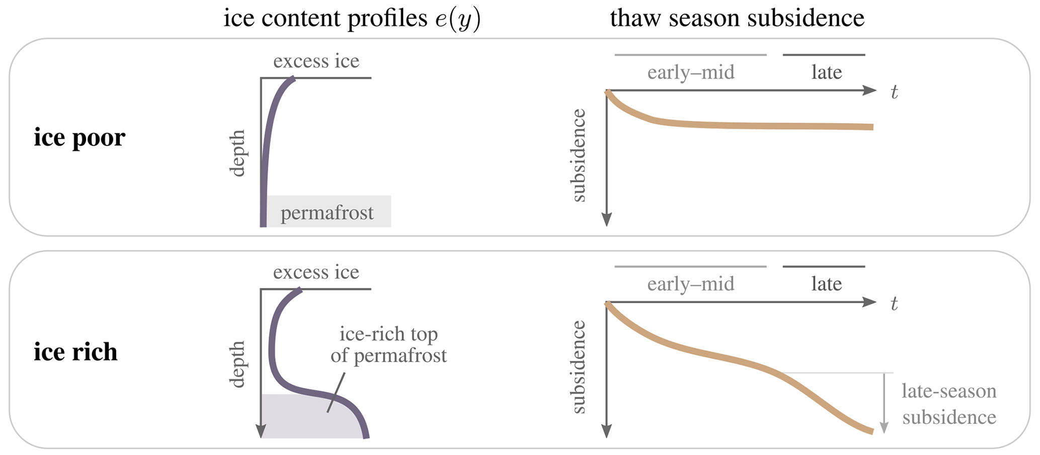
Figure 1 Late-season subsidence is predicted to be closely related to the excess ice content at the top of permafrost in an exceptionally warm (and wet) summer. When the thaw front penetrates the permafrost in the late season, the melt of excess ice in the permafrost, where present, will give rise to increased subsidence. Early-season subsidence reflects excess ice at the top of the active layer, which may also be present in units with ice-poor permafrost (top row), such as young floodplains. The subsidence time series are cumulative and relative to the beginning of the thaw season.

Here, we assess remotely sensed late-season subsidence in an exceptionally warm summer as an indicator of excess ground ice at the top of permafrost. The idea is that, towards the end of a hot summer, the thaw front can penetrate materials that were previously perennially frozen (Fig. 1). If these materials do not contain excess ground ice, we generally do not expect to observe elevated late-season subsidence. If they are rich in excess ground ice, the melt of this ice is predicted to induce a characteristic late-season acceleration of subsidence (Harris et al., 2011). Late-season subsidence is a sign that the thaw front has penetrated ice-rich materials at depth, which is difficult to observe in the field. As such, it may be a subtle (≲ 1 cm) precursor for long-term instability, or even the expression of rapid and pronounced (≳ 5 cm) thermokarst in an exceptionally warm summer. In addition to warm temperatures, wet conditions (Jorgenson et al., 2006; Shiklomanov et al., 2010; Douglas et al., 2020) and surface disturbance (J. C. Jorgenson et al., 2010; Liu et al., 2015) can also promote deep thaw, triggering late-season subsidence in ice-rich permafrost.

Late-season subsidence is a physically based indicator of top-of-permafrost excess ground ice. To sketch the physical connection, we will make the simplifying assumption that even on submonthly timescales, thaw consolidation equals the melt of excess ground ice in a given period (Morgenstern and Nixon, 1971). We further neglect summer heave (Mackay, 1983). In a simple 1D scenario, the subsidence s(t₁,t₂) between times t₁ and t₂ is then equal to the total excess ice that melts during that period:

$$\begin{array}{}\text{(1)}& {\displaystyle }s(t_{\mathrm{1}},t_{\mathrm{2}})=\underset{y_{\mathrm{f}}\left(t_{\mathrm{1}}\right)}{\overset{y_{\mathrm{f}}\left(t_{\mathrm{2}}\right)}{\int }}e\left(y\right)\mathrm{d}y,\end{array}$$

where e(y) is the excess ice content [−] per unit depth dy. y_f(t) is the depth of the thaw front relative to the surface at the beginning of the thaw season; it is assumed to be a monotonic function of t. By judicious choice of t₁ and t₂, one can determine at which depth to probe the excess ice content. By focusing on the late season, we intend to isolate the excess ice at the base of the active layer and top of the permafrost (Harris et al., 2011; Bartsch et al., 2019). Sensitivity to the excess ice at the top of the permafrost – segregated and massive ice – is important because it is the permafrost ground ice that determines the susceptibility to terrain instability (Kokelj and Jorgenson, 2013).

Remote sensing of late-season subsidence has become possible on a circumpolar scale with the advent of the Sentinel-1 InSAR satellites (Torres et al., 2012). The repeat interval of 12 d allows subseasonal variability in subsidence to be resolved (Chen et al., 2018; Bartsch et al., 2019; Rouyet et al., 2019). With other satellites, the longer repeat intervals necessitated a shallow upper limit y_f(t₁), thus precluding subseasonal separation of deeper excess ice from that in the upper active layer (Liu et al., 2015; Chen et al., 2020). Consequently, past InSAR studies have largely focused on long-term subsidence (Liu et al., 2015; Iwahana et al., 2016). This observation strategy can be used to detect ice-rich permafrost indirectly through thermokarst but presupposes prolonged degradation (Liu et al., 2015; Iwahana et al., 2016). Conversely, Sentinel-1 may allow for the detection of ice-rich permafrost within a single season through late-season subsidence, but its suitability for identifying ice-rich permafrost is unknown.

To assess the suitability of remotely sensed late-season subsidence as a permafrost ground ice indicator, we use Sentinel-1 observations near Kivalina, northwestern Alaska, from 2017–2019. The summer of 2019 was the warmest since 1980 and also wet. To determine the specificity and sensitivity of the satellite observations, we compare them to ground ice cores and to an independent ground ice map, which we derived based on manual interpretation of high-resolution optical images and field observations. Based on these assessments, we appraise the suitability and discuss the limitations of late-season subsidence as a ground ice indicator. These findings will serve to enhance the automated mapping of ground ice and anticipating terrain instability on pan-Arctic scales.

2 Study area

Our study area is located in the northwestern Alaskan Arctic, near the town of Kivalina (Fig. 2a). The surficial geology and topography are varied (DOWL Engineers, 1994; Tryck Nyman Hayes, 2006). The spectrum includes marine deposits near the mouth of the Kivalina River, various types of alluvial and colluvial sediments, and bedrock outcrops and well-drained, rubble-covered uplands. The area is underlain by warm (mean annual ground temperature of $\sim -\mathrm{3}$ ^∘C), (quasi-)continuous permafrost (Tryck Nyman Hayes, 2006). While no contemporary active layer thickness measurements are available, Shannon & Wilson, Inc. (2006) report values ranging from 0.5 to 1.0 m.

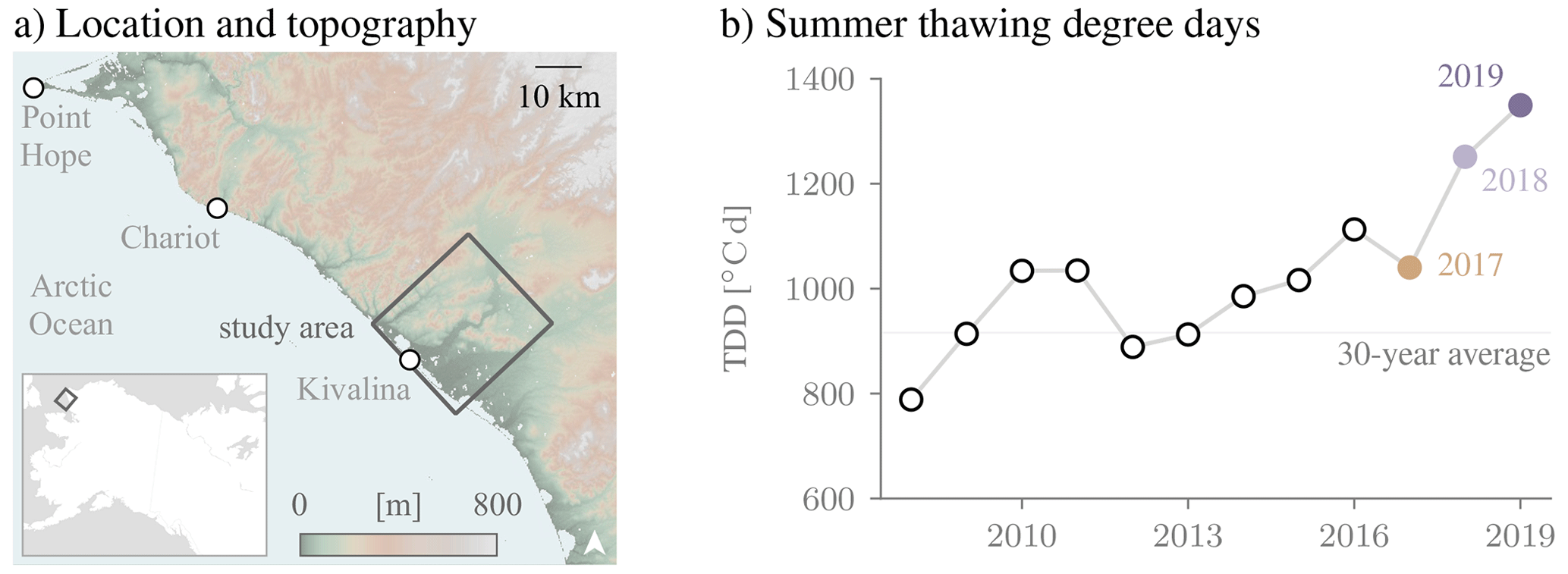
Figure 2 The Kivalina study area in northwestern Alaska (a) comprises areas of low to moderate topography (source: TanDEM-X DLR, 2020). (b) Thawing degree days (TDD) estimated from MERRA-2 air temperatures identify 2019 as an exceptionally warm summer.

Excess ground ice at the top of permafrost underlies many locations, as indicated by geotechnical investigations (Shannon & Wilson, Inc., 2006) as well as remote sensing. Geotechnical analyses have been necessitated by environmental hazards such as increasing storm surges and coastal erosion, which have been driving efforts to relocate the village from its present location on a low-lying barrier island. The 2006 master plan for the relocation planning project (Tryck Nyman Hayes, 2006) concluded that all investigated alternative sites were at least partially underlain by ice-rich permafrost. Ice wedges and ice-rich layers of segregated ice are widespread throughout the study area (Shannon & Wilson, Inc., 2006).

Meteorological conditions in the summers of 2017 to 2019 differed markedly. In western Alaska 2019 was a record warm summer. According to MERRA-2 reanalysis data (Gelaro et al., 2017; Global Modeling and Assimilation Office, 2020, shown in Fig. 2b), the thawing degree days in 2019 exceeded those of the years 2008–2017 by more than a third. Average daily temperatures in 2019 were particularly elevated in late June and early July (Fig. S1a in the Supplement), and they also remained consistently above 10 ^∘C in late August and the first half of September. The summer of 2018 was also warm but not as exceptional as that of 2019. Precipitation also varied, with 2019 being the wettest and 2018 the driest of the three (Fig. S1b).

3 Methods

3.1 Subsidence from radar interferometry

3.1.1 Sentinel-1 observations

To estimate surface displacements at a resolution of 60 m, we used Sentinel-1 observations between early June and mid-September 2017–2019. The Sentinel-1 observations (Torres et al., 2012; Copernicus Sentinel, 2020) were acquired at a frequency of 5 GHz with VV polarization in the interferometric wide mode (single-look resolution of ∼ 10 m). Acquisitions from an easterly look direction (37^∘ incidence angle; descending orbit; path 15, frame 367) were available at 12 d intervals. There was one exception in 2017, during which a gap of 18 d occurred.

3.1.2 Estimating subseasonal subsidence time series

To estimate a subseasonal displacement d time series from the Sentinel-1 observations (Copernicus Sentinel, 2020), we applied Short BAseline Subset (SBAS) processing (Berardino et al., 2002). The rationale of this Interferometric SAR (InSAR) approach is to derive displacement time series from redundant interferograms. We first formed interferograms with temporal separations of up to 24 d, using spectral diversity techniques for coregistration (Scheiber and Moreira, 2000) and removing the topographic phase contribution using the TanDEM-X DEM (Rizzoli et al., 2017; TanDEM-X DLR, 2020). After multilooking to a resolution of 60 m, we unwrapped the interferograms using SNAPHU (Statistical-Cost, Network-Flow Algorithm for Phase Unwrapping; Chen and Zebker, 2001). Ionospheric phase corrections were deemed to be unnecessary. We then estimated the displacement time series, with a temporal sampling of 12 d, from the interferogram stack. We used a weighted least-squares approach based on the singular value decomposition (Berardino et al., 2002), with the weights determined by the Cram'er–Rao phase variance estimate (Tough et al., 1995).

The time series are reported as displacements d along the line-of-sight direction, with positive values corresponding to increasing distance. Owing to the hilly terrain, we chose not to convert them to vertical displacements. However, we did not discern aspect-dependent trends that are associated with downslope movements. If downslope motion were comparable to surface-perpendicular motion, the west-facing slopes would show greater line-of-sight displacements than the east-facing slopes. For simplicity's sake, we will refer to displacements with increasing distance as subsidence. The time series record the cumulative subsidence since the first radar observation.

3.1.3 Referencing and assessing its quality

To reduce long-wavelength atmospheric errors in the subsidence observations, we spatially referenced the raw time series at multiple locations with outcropping bedrock or a thin rubble veneer. These locations were assumed to be stable (Reger and Solie, 2008; Antonova et al., 2018).

To assess the quality of the referencing, we chose eight bedrock validation points distributed across the study region. Assuming these points remain stable, the subsidence observations at these locations are a measure of the observational uncertainty. This uncertainty estimate subsumes decorrelation errors and uncompensated for atmospheric contributions under a single number.

3.1.4 Late-season subsidence from spline fitting

We estimated the late-season subsidence d_l by fitting spline basis functions to the referenced subsidence time series. The advantage of fitting a flexible and yet simple spline function is that measurement noise, such as residual atmospheric errors, can be reduced (Berardino et al., 2002).

To capture a range of subseasonal subsidence patterns, we used three cardinal quadratic B splines for the subsidence rate (first derivative), corresponding to the cubic spline basis functions for the subsidence time series shown in Fig. 3a. For each pixel, we estimated the three coefficients by ordinary least squares.

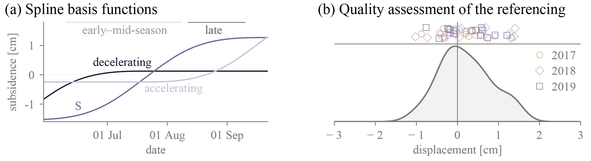
Figure 3 Late-season and early–mid-season subsidence were reconstructed by spline fitting and their accuracy assessed at stable validation points. (a) Three cubic spline basis functions, corresponding to decelerating, S-shaped, and accelerating subseasonal subsidence; for display purposes, we normalized them so that the peak subsidence rate is 1 mm/d. (b) Reconstructed displacements over the validation points during the early-to-mid-season and late season (d_e and d_l, respectively; positive values corresponding to subsidence). Individual values for all points and years shown at the top and a kernel density estimate of the distribution below.

The late-season subsidence d_l was defined to be the cumulative subsidence between 10 August (t₁) and 10 September (t₂) for all years. We chose t₁ such that the thaw front in an exceptionally warm summer could plausibly have reached the average long-term permafrost table. To test the sensitivity of the d_l estimates to this choice, we also computed d_l starting 10 d earlier or later. The end point t₂ was chosen to minimize the confounding impact of diurnal frost heave (Chen et al., 2020). We expect the thaw front to be within < 5 % of its seasonal maximum at t₂. For the specified values of t₁ and t₂, we derived d_l from the spline fit.

We also estimated total subsidence during the early and middle thaw season (10 June to 10 August), d_e. While d_e is not expected to contain direct information about permafrost ground ice, being sensitive to soil texture and interannual variations in active layer moisture (Lewkowicz, 1992; Harris et al., 2011), it provides a simple reference for assessing the late-season speed-up characteristic of melting top-of-permafrost excess ground ice.

3.2 Assessment with independent ground ice data

3.2.1 Manual mapping

We assessed the suitability of late-season subsidence as an indicator of permafrost ground ice content by comparing the InSAR observations to an independently derived ground ice map, published as Zwieback (2020a). The map comprised two primary categories: ice rich and ice poor. To assess the sensitivity and specificity, we computed the observed late-season subsidence distributions conditional on the location being ice rich and ice poor, respectively.

The independently derived ground ice map was obtained using manual interpretation and expert knowledge, drawing on field observations and high-resolution (∼ 1 m) satellite imagery. The mapped focus area, 8 km by 8 km in size, was chosen because of the wide range of ecotypes and the availability of field observations. A drawback of the map is its gaps, because we classified the ground ice content of 19 % of the area as indeterminate. Furthermore, 6 % of the area was discarded in the comparison to avoid unrepresentative values over lakes and infrastructure.

The key considerations in the manual mapping were as follows.

1. Ice-rich permafrost was assigned to ecotypes where high-resolution imagery and field observations revealed direct indicators of excess ice at the top of permafrost. Ice wedge polygons – some only barely visible or inconspicuous except along lakeshores and beaded streams, others visibly in an advanced state of degradation – are widespread (Fig. 4). They are abundant in old alluvial and lacustrine deposits (DOWL Engineers, 1994; Shannon & Wilson, Inc., 2006) as well as in colluvial sediments that are rich in retransported silt (DOWL Engineers, 1994).

2. A major caveat is that the presence of ice wedges provides no direct information on the ice content in the polygon interiors. However, previously taken cores (by Shannon & Wilson, Inc., 2006; to be discussed later) from centres in various terrain units were ice rich, and the presence and ongoing expansion of thermokarst ponds and lakes also provide support for this assumption.

3. Pingos in drained lake basins are also direct indicators of excess ground ice (Mackay, 1973).

4. Exposed bedrock and rubble-covered surfaces (Fig. 4b) were classified as ice poor. This classification is generally supported by geotechnical investigations and field evidence from the study area (Pewe et al., 1958; DOWL Engineers, 1994). Deviations from this general pattern cannot be excluded (Robinson and Pollard, 1998; French and Shur, 2010).

5. Active and recent inactive floodplains were categorized as ice poor (Fig. 4a; DOWL Engineers, 1994) because near-surface permafrost, where present, is too young for abundant ground ice to have aggraded (Jorgenson et al., 1998). We did not observe any indications of abundant excess ground ice in these ecotypes.

6. Such indirect indicators as vegetation cover and surficial geology were used to classify areas as ice rich where similar adjacent areas were clearly ice rich. For instance, if polygons were visible over 80 % of an alluvial deposit, the entire deposit was classified as ice rich (Fig. 4a).

7. The ice content of the remaining locations was deemed to be indeterminate. The majority of these locations are in uplands and on hillslopes, where ice content is inherently variable (Morse et al., 2009). In Fig. 4b, the areas above the clearly ice-rich toe and midslope deposits (Fig. 4b) lack visible manifestations of ice-rich permafrost, but it is known that some are ice rich (Shannon & Wilson, Inc., 2006). Floodplain deposits of intermediate age (between recent inactive and old abandoned floodplains) were also classified as indeterminate (Jorgenson et al., 1998).

.

Figure 4 Manual classification into ice-rich and ice-poor terrain relied on visible manifestations of ground ice. (a) Ice-rich predominantly alluvial deposits are on the left, as indicated by ice wedge polygons (inundated troughs, heterogeneous vegetation communities, cut bank morphology), whereas the active floodplain of the Wulik River on the right is ice poor. (b) Hillslope sequence with the ice-poor nature of the ridge (right) being indicated by bedrock and rubble; there is little evidence for or against ice richness near the top of the slope (middle); the midslope hosts abundant but faint ice wedge polygons (inset). For visual display purposes, the boundaries have been shifted. The two locations are identified in Fig. 7b

The mapping process is inherently subjective. The discretization of top-of-permafrost excess ground ice into a limited number of categories presents challenges (Tryck Nyman Hayes, 2006; Paul et al., 2021). The most difficult decisions were about where to draw the line between the ice-rich/ice-poor category and the indeterminate category.

3.2.2 Cores

We also compared the late-season subsidence observations to geotechnical assessments of permafrost ground ice content from > 3 m deep cores. The cores were taken in 2005 by Shannon & Wilson, Inc. to investigate the suitability of three proposed relocation sites for Kivalina (Shannon & Wilson, Inc., 2006). Where ice wedge polygons were discernable at the surface, cores were taken from the polygon centres (in one case: centre and wedge).

Ice-rich permafrost was encountered underneath all sites, but the Tatchim Isua site (Fig. 5) also encompassed an ice-poor bench. The ice-rich nature of the area surrounding the ice-poor bench was not evident at the surface; it only became conspicuous at the surface ∼ 300 m upslope, in the form of faint ice wedge polygons (Shannon & Wilson, Inc., 2006).

Although coring is the most reliable method for determining ground ice content, the spatial and temporal representativeness of the cores needs to be considered. The point observation a single core represents could paint a misleading picture of ground ice content (Morse et al., 2009; Kanevskiy et al., 2017) when compared to a ∼ 60 m resolution cell. The cores were further taken a decade before the remote sensing observations. However, none of the locations showed signs of severe disturbance, and the observed thickness of the ice-rich layer at the top of permafrost, where present, exceeded 30 cm (Shannon & Wilson, Inc., 2006).

We classified the cores as ice poor and ice rich based on the descriptions in the geotechnical report (Shannon & Wilson, Inc., 2006). The ground ice content of each core was summarized verbally as ice rich or ice poor, complemented by pictures and estimates of the visible ice content. All cores but one were ice rich with visible ice contents > 30 % in the forms of segregated and wedge ice. The only ice-poor core, from the bench, was a gravelly soil grading into weathered bedrock (5 % visible ice content in joints). Two cores taken from within the same ice wedge polygon were combined for the comparison exercise. Table S1 in the Supplement summarizes the locations and ground ice properties of all 13 coring locations.

4 Results

4.1 Spatial and temporal variability of late-season subsidence

4.1.1 Regional variability

The observed late-season subsidence in our study area showed two distinct modes in 2019 (Fig. 5a). One corresponded to no or very small subsidence (−1 to 1 cm). The other corresponded to regions with elevated subsidence (4–8 cm) in 2019. In 2017, the subsidence in these regions was lower (1–4 cm).

There were no notable instances of pronounced negative late-season subsidence estimates in any of the years. Negative estimates correspond to heave during the late season (10 August to 10 September). Small negative values ($\sim -\mathrm{1}$ cm) occurred in all years. These need to be interpreted in relation to the observational accuracy. Observations at the validation points (bedrock locations shown as circles in Fig. 5) correspond to a root-mean-square accuracy of 0.6 cm. The distribution shown in Fig. 3b encompasses estimates of either sign with a magnitude that is small compared to the observations in the subsiding areas.

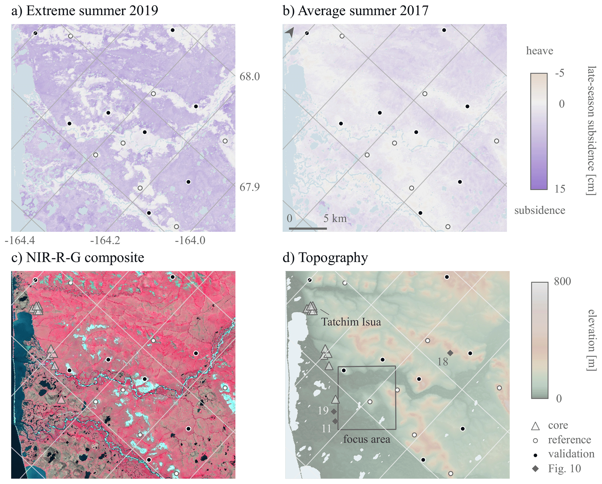
Figure 5 Remotely sensed late-season subsidence d_l within the study area, defined in Fig. 2; (a) d_l in the exceptionally warm summer of 2019; (b) d_l in the average summer of 2017. Positive values correspond to subsidence between 10 August and 10 September and negative values to heave during the same period. Missing values are shown in light blue. (c) Sentinel-2 false-colour composite image (Copernicus Sentinel, 2020); (d) topography estimated from the TanDEM-X DEM. The reference and validation points (Sect. 3.1.3) for the Sentinel-1 subsidence estimates are indicated by white and black circles, respectively; the locations of the ground ice cores are shown by triangles; the labelled diamonds refer to points shown in Fig. 10. The focus area for manual mapping and the Tatchim Isua candidate relocation site are shown in (d).

Late-season subsidence varied with topographic position and surficial geology. Elevated late-season subsidence exceeding 3 cm was found in low-lying areas including old alluvial deposits and drained lake basins (Fig. 5a–b). Many hillslopes also featured elevated late-season subsidence in 2019. Conversely, late-season subsidence was consistently low in elevated uplands (bedrock or talus without vegetation cover) and along rivers (e.g. recent floodplains without or with dense vegetation cover.)

4.1.2 Temporal variability

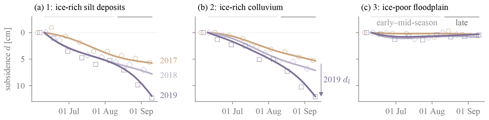
The late-season subsidence exhibited more year-to-year variability than the early–mid-season subsidence (Figs. 5, S2). Three examples in Fig. 6 illustrate the inter-annual variability of the subsidence time series.

A late-season acceleration of subsidence in 2019 was observed in two locations that were independently determined to be ice rich (Fig. 6a and b). According to the radar observations, the rate of subsidence more than doubled in the late season. The rate and the total subsidence of ∼5 cm during the late season is approximately a factor of 3 smaller in the years 2017 and 2018.

For the ice-poor floodplain in Fig. 6c, the interannual variability in late-season subsidence was less than 1 cm. The magnitude of the late-season subsidence was always small, comparable to the observational uncertainty in all years.

Figure 6 Cumulative subseasonal subsidence (line: spline fit, markers: unconstrained) from all 3 years. The late-season subsidence (10 August–10 September) is highlighted for the year 2019 in (b). The locations of (a)–(c) are shown in Fig. 7c.

4.2 Assessing the suitability as an indicator of top-of-permafrost ground ice

4.2.1 Suitability in an exceptionally warm summer

Late-season subsidence in the hot and wet summer of 2019 was markedly different for ice-rich and ice-poor areas (Fig. 7a). It exceeded 4 cm at all cored locations rich in top-of-permafrost ground ice. For the ice-rich areas, as determined by independent manual mapping, d_l varied between 4 and 8 cm (5th and 95th percentiles; Fig. 7c–d). For ice-poor areas the 5th–95th percentile range was −1 to 2 cm. Only in the extreme tails (2 %) do the distributions overlap, ensuring a robust separability of the two classes. Based on the distributions, we applied a threshold of 2.5 cm to separate ice-rich from ice-poor permafrost (Fig. 7e).

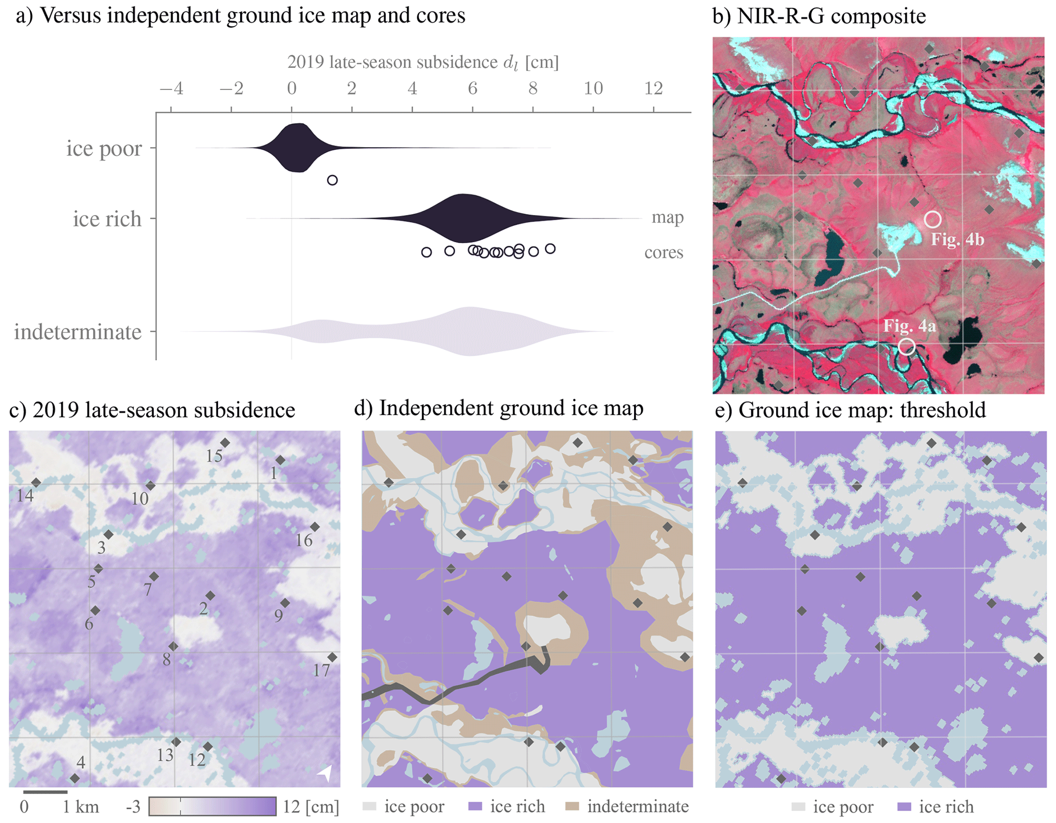
Figure 7 Assessment of late-season subsidence with respect to an independent ground ice map of the focus area defined in Fig. 5. (a) Kernel density distribution of d_l in 2019 over areas independently determined to be ice rich and ice poor. The markers just below the kernel density estimates show the observations at the boring locations (triangles in Fig. 5). (b) Sentinel-2 false-colour composite (Copernicus Sentinel, 2020) for the focus area defined in Fig. 2. (c) The estimated d_l, (d) the independently determined ground ice map, and (e) the ground ice classification obtained by thresholding d_l. The diamonds indicate points mentioned in Figs. 6 and 10.

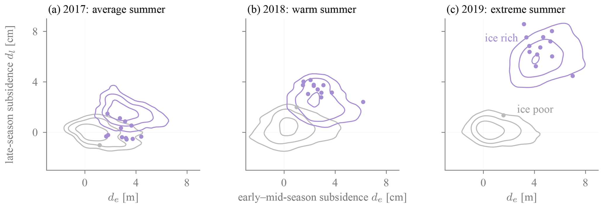
Figure 8 Contour plot of a kernel density estimate of the early–mid-season and late-season subsidence for ice rich (purple) and ice poor (grey), as determined independently by manual mapping (Fig. 7d). The markers correspond to the values observed at the location of the ice cores (triangles in Fig. 5). Negative values, corresponding to heave, are of comparable magnitude to the referencing accuracy of ∼ 1 cm.

The separability based on the 2019 late-season subsidence d_l is better than that based on the early–mid-season subsidence d_e. The d_e distributions of ice-rich and ice-poor areas overlap (Fig. 8c), whereas the d_l distributions are concentrated around two separate peaks (see also Fig. 7a). When the start of the late-season period is pushed backward, the separability based on d_e improves, whereas that based on d_l decreases (Fig. S3).

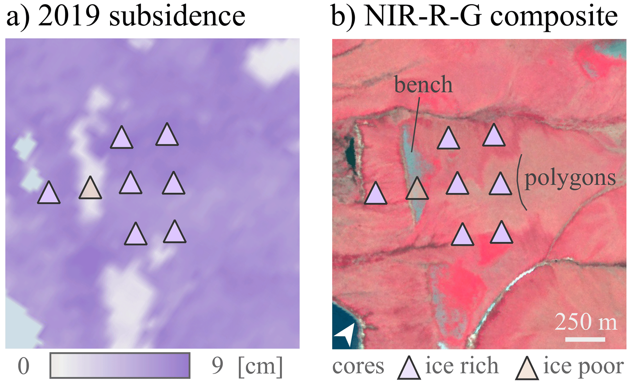
Figure 9 Late-season subsidence in 2019 (a) at the Tatchim Isua site (see Fig. 5 for its location) is smaller at the site of the gravelly bench, which appears grey in the false-colour composite (courtesy of Planet Labs, Inc.; Planet Team, 2020) in (b) than the areas further upslope (right) and downslope (left). The triangles mark the location of the ice cores, with the colour indicating their ice content. Ice wedge polygons were observed in the field ∼ 300 m upslope from the bench.

The candidate relocation site Tatchim Isua was characterized by a narrow zone with low late-season subsidence (Fig. 9). This ∼ 100 m wide zone largely coincides with the gravel-covered bench that a single core from 2005 (Table S1) indicates to be ice poor (Shannon & Wilson, Inc., 2006). Late-season subsidence was elevated (∼ 7 cm) at the location of the seven cores further downslope or upslope. All cores contained ice-rich materials at the top of permafrost, but in the field the ice-rich nature was not readily apparent at the surface near the proximal coring locations (Shannon & Wilson, Inc., 2006).

Further examples from a range of geologic settings serve to illustrate the suitability of d_l for identifying ice-rich permafrost. Figure 10a–d show instances of ice-rich permafrost with ice wedge polygons. They all exhibited elevated d_l of 4–8 cm, corresponding to an increased subsidence rate during the late season. Conversely, the observed subsidence was below 1 cm for the points shown in Fig. 10i–l, which were independently determined to be poor in ground ice.

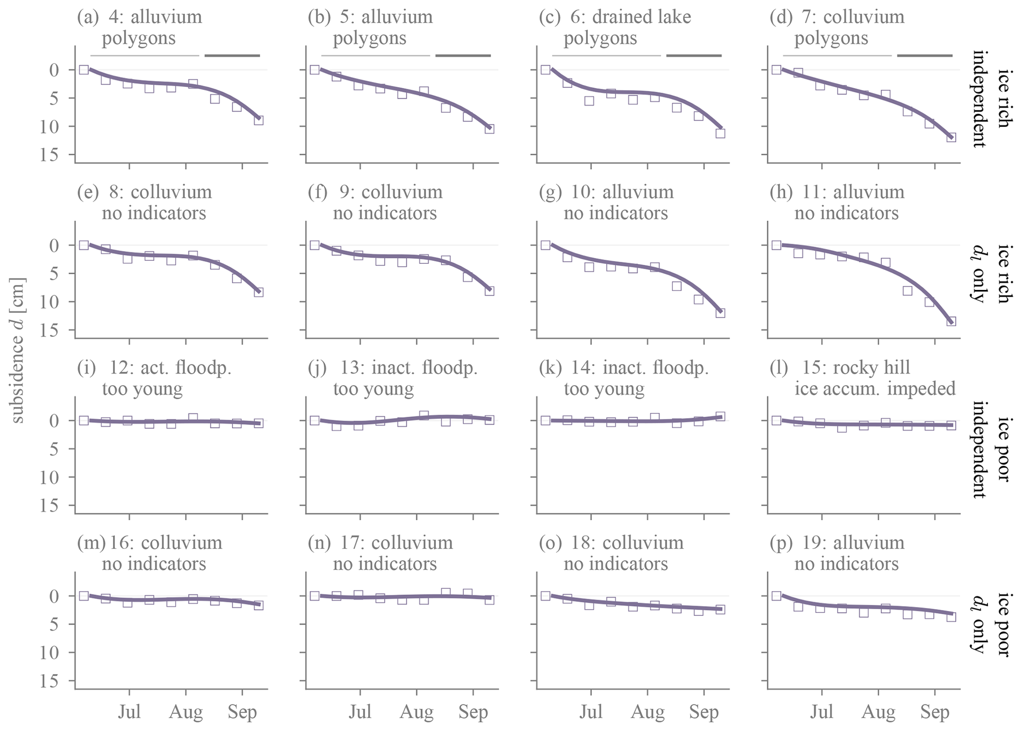
Figure 10 Subsidence time series (line: spline fit, markers: unconstrained) from 2019 for points shown in Figs. 7c and 5d. First row (a–d): points that were independently determined to be ice rich; second row (e–h) indeterminate according to manual mapping, but d_l>2.5 cm indicates they are ice rich; third row (i–l): independently determined to be ice poor; fourth row (m–p): indeterminate according to manual mapping, but d_l indicates they are ice poor.

The most interesting cases are those 19 % of the area where the manual ground ice mapping was indeterminate because there was no strong evidence for either category. They exhibited a bimodal distribution of d_l (Fig. 7a). The larger mode d_l were ∼5 cm, comparable to those of ice-rich areas. Examples include colluvial hillslope deposits without conspicuous ground ice indicators (Fig. 10e–h). The characteristic late-season acceleration in subsidence leading to elevated d_l∼5 cm uniquely indicates that the top of the permafrost is ice rich. The smaller mode d_l∼1 cm roughly matches the observations over ice-poor terrain. The negligible subsidence observed at the locations shown in Fig. 10m–p suggests that the materials that thawed late in summer contained little excess ice.

4.2.2 Suitability in cooler years

In the average year of 2017, the suitability was reduced because the late-season subsidence distributions of ice-rich and ice-poor regions overlapped substantially (Fig. 8a). The late-season subsidence d_l of 80 % of the terrain that was mapped to be ice rich and all the ice-rich coring locations was less than 2 cm. On average, it was 4 cm, or a factor of 5 smaller, than during 2019 (standard deviation: 1 cm).

In the warm summer of 2018, the separability based on the d_l distributions was intermediate. The distributions overlapped at the 10 % level (Fig. 8b), compared to 2 % in 2019. This is largely due to the smaller late-season subsidence of ice-rich terrain compared to the exceptionally warm summer of 2019.

5 Discussion

5.1 Suitability for identifying top-of-permafrost excess ground ice

Comparing the late-season subsidence to the independently determined ground ice map and the ice cores, we note that ice-poor and ice-rich permafrost are distinguishable in the exceptionally warm summer of 2019 (Fig. 7). Ice-poor areas were stable, whereas ice-rich areas exhibited pronounced (∼ 5 cm) late-season subsidence (Fig. 10).

The late-season speed-up in subsidence is interpreted as the thaw front penetrating ice-rich materials at the top of permafrost (Shur et al., 2005; French and Shur, 2010). A characteristic feature is that the subsidence rate increased up to 5-fold in late summer (Fig. 10). Harris et al. (2011) interpreted the late-season acceleration observed in situ in Svalbard by the sharp contrast in excess ice between the ice-rich layer and the materials above. In practical terms, the acceleration increases the robustness of the separability with respect to the chosen starting day of the late season period (Fig. S3), thus facilitating the identification of ice-rich materials at the top of the permafrost. If the ice-rich layer is thick, the late-season acceleration in subsidence can be a precursor for long-term terrain instability (Kanevskiy et al., 2017).

Inter-annual variability in late-season subsidence of ice-rich areas poses challenges for ground ice mapping. Potential drivers of inter-annual variability and trends include surface changes (e.g. soil moisture, disturbance, snow) and variable meteorological conditions such as precipitation (Shiklomanov et al., 2010; Bartsch et al., 2019; Douglas et al., 2020). In contrast to the exceptionally warm and wet summer of 2019, the limited late-season subsidence of ∼ 2 cm in the warm summer of 2018 in the ice-rich area shown in Fig. 6a indicates the thaw front did not sufficiently penetrate into the ice-rich materials. That the identification strategy presupposes an initial degradation of excess ground ice constitutes its biggest limitation.

5.2 Limitations

The excellent separability in our study area in the exceptionally warm summer does not imply that interferometric observations of late-season subsidence are a universally applicable basis for mapping ice-rich permafrost. Limitations arise from observational uncertainties and from the imperfect sensitivity and specificity of subseasonal subsidence as an indicator of top-of-permafrost excess ground ice.

5.2.1 Observational uncertainties

Observational uncertainties chiefly arose from errors in the referencing, dominated by uncompensated for atmospheric contributions and from location-specific systematic and random errors.

The errors due to imperfect referencing were determined to be substantially smaller (1 cm; Fig. 3b) than the typical difference in late-season subsidence between ice-rich and ice-poor permafrost terrain (5 cm; Fig. 7a).

This uncertainty metric does not account for systematic biases associated with changes in soil or vegetation moisture, as was obtained from rocky, non-vegetated surfaces. Soil moisture commonly increases toward the end of the thaw season, which would correspond to a spurious subsidence signal (De Zan et al., 2015). However, the worst-case estimates of the bias (∼ 1 cm at C-band) are a factor of 5 smaller than the late-season subsidence observations (Zwieback et al., 2017). Vegetation moisture in shrubs will decrease with senescence, corresponding to a spurious heave signal of ∼ 1 cm (Zwieback and Hajnsek, 2016). The persistently small magnitude of the displacement estimates over shrub-covered inactive floodplains (Fig. 5) indicates that these systematic errors were not a major confounding factor in the present study. However, dedicated in situ observations are needed to accurately characterize the observational uncertainties. We expect these errors to be greater in densely vegetated, often discontinuous, permafrost (Wang et al., 2020).

5.2.2 Limitations of late-season subsidence for identifying top-of-permafrost ground ice

The ample suitability of late-season subsidence for mapping ice-rich permafrost that we identified in the study area was arguably promoted by the exceptionally warm and wet summer of 2019. In less propitious circumstances, its sensitivity and specificity may be reduced.

Its sensitivity is impaired when excess ground ice does not manifest as elevated late-season subsidence. Such false negatives occurred for instance in the warm summer of 2018 but not in 2019 (Fig. 8b), indicating that in 2018 the thaw front did not penetrate substantially into the ice-rich materials in the upper permafrost. Limited late-season subsidence in warm summers is promoted by the low to moderate ice contents above the ice-rich materials, i.e. the lower active layer and the transient layer (Shur et al., 2005). Consequently, identifying ice-rich permafrost using late-season subsidence calls for exceptionally warm summers such as 2019.

False negatives – even in an extremely warm summer – are expected to occur most commonly in the discontinuous and sporadic permafrost zone. There, disturbances such as forest fires are more likely to have obliterated the ecosystem-protected or ecosystem-driven perennial ground ice near the surface (M. T. Jorgenson et al., 2010; Kanevskiy et al., 2012, 2014; Paul et al., 2021), but see Burn (1997). Ice-rich permafrost may occur at depth, perhaps under a thick talik. The thermal regime of such permafrost is more complex (M. T. Jorgenson et al., 2010; Connon et al., 2018), and melt-induced subsidence does not necessarily occur primarily at the end of the thaw period. The sensitivity may further be diminished by the retardation of thaw consolidation due to inefficient drainage of the excess meltwater (Morgenstern and Nixon, 1971) or by sinkhole formation and piping underneath cohesive materials such as peat (Osterkamp et al., 2000). In such challenging environments, subsidence-based ground ice mapping will benefit most from synergies with complementary mapping approaches.

The specificity is impaired when late-season displacements are not due to melt of top-of-permafrost ground ice. Elevated late-season subsidence may reflect ice content at the bottom of the active layer. Cold permafrost and ample moisture supply promote ice segregation at the base of the active layer, with a seamless transition in ground ice content to the ice-rich upper permafrost (Mackay, 1981). Problems could further be caused by late-season deformation related to processes such as organic soil compaction and mass loss, or downslope transport (Stephens et al., 1984; Roulet, 1991; Matsuoka, 2001; Gruber, 2020; Zhang et al., 2020). It will be beneficial to incorporate expert knowledge and to exploit the characteristic late-season acceleration shown in Fig. 6a–b in order to robustly identify ice-rich permafrost.

A final limitation of this study and the preceding discussion is that the complexity of ground ice was simplified to just two categories: ice rich and ice poor. In reality, however, excess ground ice content is a continuous parameter (Morse et al., 2009; Kanevskiy et al., 2012; Paul et al., 2021) whose magnitude could be constrained using late-season subsidence observations. A big challenge, the sub-resolution spatial variability of ground ice, is exemplified by ice-wedge polygons. To what extent do the satellite observations reflect the wedges and the polygon interior, and how does it vary with factors such as ice content of the centres and the thickness distribution of the protective layer above the wedges? Quantitative answers will require densely sampled ground ice cores (Morse et al., 2009; M. T. Jorgenson et al., 2010).

5.3 Enhancing automated ground ice mapping

Late-season subsidence may enhance the automated mapping of permafrost ground ice. Remotely sensed late-season subsidence can be mapped on pan-Arctic scales, thanks to the global availability of Sentinel-1 data (Torres et al., 2012). A further practical advantage is that it lends itself to automation, as no manual interpretation and no calibration using in situ cores are required. To automate the specification of the late-season period, globally available reanalysis data could be considered. Despite the potential for automation, we believe that the greatest potential lies in its synergistic use with expert knowledge, field observations, and complementary mapping approaches.

Incorporating external constraints and expertise will be essential to counteract weaknesses of remotely sensed late-season subsidence. Site knowledge is indispensable for interpreting the stratigraphic complexity and sub-resolution variability of ground ice conditions. Most importantly, independent observations will be needed to estimate excess ice at depth and thus constrain total ice contents. External data can further assist in densely vegetated areas with larger errors (Wang et al., 2020) and mitigate false negatives when the thaw front fails to penetrate deep into the ice-rich materials (Shur et al., 2005).

Late-season subsidence is complementary to state-of-the-art mapping approaches based on visible manifestations of ground ice and indirect associations with vegetation cover or topographic variables. In addition to validating existing maps such as the coarse-scale product by O'Neill et al. (2019), late-season subsidence can be used synergystically in future ground ice mapping efforts. The greatest contribution of late-season subsidence will likely be where field observations are sparse or where ground ice is indistinct and poorly correlated with surface characteristics. Examples include uplands and hillslopes (Fig. 9), as well as areas underlain by ice wedges from the early Holocene or the Pleistocene (Pewe et al., 1958; Dredge et al., 1999; Reger and Solie, 2008; Morse et al., 2009; Jorgenson et al., 2015; Farquharson et al., 2016).

6 Conclusions

We set out to assess the suitability of remotely sensed late-season subsidence for identifying ice-rich materials at the top of permafrost. We predicted that ice-rich permafrost would become detectable by enhanced subsidence toward the end of an exceptionally warm summer. Our assessment was based on the comparison of Sentinel-1 satellite observations from 2017–2019 with independent ground ice data in northwestern Alaska. Our principal findings and conclusions are as follows.

1. In the exceptionally warm and wet summer of 2019, the InSAR-derived late-season subsidence observations were large (∼ 4–8 cm) in areas that were independently determined to be rich in top-of-permafrost ground ice. Conversely, the observed late-season subsidence was consistently small (−1 to 2 cm) in ice-poor areas.

2. Distinguishing ice-rich from ice-poor terrain worked best in the exceptionally warm and wet summer, as the respective late-season subsidence distributions overlapped by less than 2 %. In the preceding summers the overlap was 10 % or larger.

3. The suitability of late-season subsidence as an indicator that top-of-permafrost excess ice will not always be as high as in this study. The greatest drawback is the lack of sensitivity when the thaw front does not penetrate deep into the ice-rich layers, but in suitable terrains this limitation can be mitigated through the use of imagery acquired during an exceptionally warm and wet summer.

4. Remotely sensed late-season subsidence complements established techniques for estimating ground ice contents, such as manual mapping approaches that exploit visible manifestations of ground ice and indirect associations with surface characteristics. Because late-season subsidence is insensitive to excess ice at depth, it will be essential to incorporate geological reasoning and indirect associations established using field observations for estimating total ice contents.

5. In summary, late-season subsidence can enhance the mapping of permafrost excess ground ice and the susceptibility to terrain instability. Its practical advantages include the pan-Arctic availability of data, the ease of automation, the independence from costly in situ observations, and its applicability in absence of visible manifestations of ground ice. Late-season subsidence in a warm and wet summer may be relatively small, but it can serve as an observable precursor for much larger terrain changes.

Pan-Arctic expansion of ground ice mapping using late-season subsidence is timely and societally relevant. It is timely because of the widespread warming and accelerating degradation of permafrost. It is relevant because we lack accurate, fine-scale ground ice maps over essentially the entire Arctic. Late-season subsidence observations can make a vital contribution to anticipating terrain instability in the Arctic and to sustainably stewarding its vulnerable ecosystems.