the Creative Commons Attribution 4.0 License.
the Creative Commons Attribution 4.0 License.
 | 11 Jan 2021
New insights into radiative transfer within sea ice derived from autonomous optical propagation measurements
Lovro Valcic
Simon Lambert-Girard
Mario Hoppmann
The radiative transfer of shortwave solar radiation through the sea ice cover of the polar oceans is a crucial aspect of energy partitioning at the atmosphere–ice–ocean interface. A detailed understanding of how sunlight is reflected and transmitted by the sea ice cover is needed for an accurate representation of critical processes in climate and ecosystem models, such as the ice–albedo feedback. Due to the challenges associated with ice internal measurements, most information about radiative transfer in sea ice has been gained by optical measurements above and below the sea ice. To improve our understanding of radiative transfer processes within the ice itself, we developed a new kind of instrument equipped with a number of multispectral light sensors that can be frozen into the ice. A first prototype consisting of a 2.3 m long chain of 48 sideward planar irradiance sensors with a vertical spacing of 0.05 m was deployed at the geographic North Pole in late August 2018, providing autonomous, vertically resolved light measurements within the ice cover during the autumn season. Here we present the first results of this instrument, discuss the advantages and application of the prototype, and provide first new insights into the spatiotemporal aspect of radiative transfer within the sea ice itself. In particular, we investigate how measured attenuation coefficients relate to the optical properties of the ice pack and show that sideward planar irradiance measurements are equivalent to measurements of total scalar irradiance.
- Article
(7114 KB) - Full-text XML
- BibTeX
- EndNote


The optical properties of the sea ice covering the polar oceans are a crucial parameter in the Earth's climate system (Grenfell et al., 2006; Perovich et al., 2007). Reflection and transmission of sunlight by sea ice determine the partitioning of shortwave radiative energy, in particular the reflection of incident irradiance back into the atmosphere (Curry et al., 1995; Perovich, 1990). Light transmitted through the ice cover does not only heat the underlying ocean (Steele et al., 2010), but also provides energy for the ice-associated ecosystem (Assmy et al., 2017; Leu et al., 2010). With thinner and younger ice (Haas et al., 2008; Renner et al., 2014) covering a smaller part of the ocean due to anthropogenic climate change (Serreze et al., 2007; Stroeve et al., 2012), the relative importance of the shortwave energy budget is increasing.
Optical properties of sea ice have been most frequently determined using measurements above and below the ice (Grenfell et al., 2006; Grenfell and Maykut, 1977; Perovich et al., 1998; Eicken and Salganek, 2010). Despite recent efforts to increase the number of such measurements by means of robotic platforms (Katlein et al., 2019, 2015, 2017; Nicolaus and Katlein, 2013), these methods only provide bulk properties that do not resolve vertical variations of sea ice optical properties. Optical properties within the ice have so far mostly been determined by the use of inverse radiative transfer models which fit a vertical profile of optical properties to observations above and below the ice (Ehn and Mundy, 2013; Ehn et al., 2008b; Light et al., 2008). Furthermore, optical properties have been derived using various techniques of analyzing extracted ice samples in laboratory setups (Grenfell and Hedrick, 1983; Katlein et al., 2014b; Light et al., 2015). Extraction of samples however is not only destructive to the natural sea ice environment, but samples also often undergo quite dramatic physical changes such as brine drainage or freezing between sample extraction and analysis in the lab.
Ehn and Mundy (2013), Ehn et al. (2008a), Light et al. (2008), Xu et al. (2012), and Pegau and Zaneveld (2000) used vertically profiling light sensors to extract radiance or irradiance profiles and attenuation coefficients within holes drilled into the ice. Voss et al. (1992), Maffione et al. (1998), and Zhao et al. (2010) used active measurements in drilled ice holes to measure the point spread function, beam spread function and horizontal light attenuation. These methods have in common that they have to be operated manually and thereby take significantly more resources compared to continuous measurements on automated platforms.
Autonomous continuous and vertically resolved optical measurements within the interior of sea ice have the potential to give a more comprehensive view on radiative transfer processes within the ice itself. They can provide closer bounds on the inherent optical properties of the ice interior, and – if combined for example with commonly available temperature chains – also provide new impulses towards the improvement of structural optical models. Light sensor chains are also the least invasive way to perform such measurements, while the small size also minimizes effects of self-shadowing. Moreover, recording data throughout the entire seasonal cycle allows for a better understanding of the seasonal evolution of the ice and how parameterizations for large-scale models can be optimized. Multispectral optical data also allow for the detection of ice algae growing within the sea ice (Mundy et al., 2007; Lange et al., 2016; Katlein et al., 2014a).
Here we present the concept, design and first results of a new autonomous in-ice light sensor chain that is able to provide multispectral in-ice light data at a significantly higher spatial and temporal resolution than previously feasible. Hourly measurements of multispectral in-ice sideward planar irradiance at a vertical resolution of 5 cm were acquired from a prototype system that was deployed in August 2018 close to the geographic North Pole. In addition to the description of the instrument itself, and a detailed analysis of this dataset, we also link the results to the physical background necessary for a proper interpretation of its data. Finally, we discuss advantages and limitations, and we highlight its scientific potential towards future applications.
2.1 The chain design
To measure vertical irradiance profiles within the ice, we build on years of experience in the field of ice temperature measurements using thermistor chains (Perovich and Richter-Menge, 2006; Richter-Menge et al., 2006; Planck et al., 2019; Jackson et al., 2013; Hoppmann et al., 2015). These chains provide an easily deployable tool for autonomous measurements of the in-ice temperature field and the thermal properties of the ice column, out of which ice thickness and snow depth can be derived. Only recently these systems have transitioned from traditional analog thermistor sensors to a chain of digital temperature sensors mounted on flexible printed circuit boards similar to the design of LED lighting strips (Jackson et al., 2013).
For this light sensor chain design, we replaced the digital temperature sensors with multispectral light sensors protected by transparent heat shrink tubing. This analogous design provides the same advantage of easy deployment through a 5 cm (2 in.) diameter hole combined with a rather rugged form factor without protruding parts. The prototype chain presented here was equipped with 48 sensors at 5 cm spacing resulting in a total chain length of 2.35 m. Longer chains, more sensors and different sensor spacing can be implemented depending on needs. The chain can be deployed through any kind of ice. While temperature sensor chains are crucially dependent on refreezing of the hole around the chain, the optical sensors are less sensitive to a potential distance to the ice, as the effects of a small hole on the in-ice light field are compensated for by the strong multiple scattering in the ice and the large sideward viewing angle of the sensors as long as the topmost dry part is refilled with drill cuttings after the chain deployment.
Measured data were sent via an Iridium Short Burst Data (SBD) satellite link requiring data transfer of around 65 kB per day for the hourly sampling schedule.
2.2 The multispectral irradiance sensor
To achieve a low total system cost and to maintain the small and compact form factor, we make use of a sensor initially designed for color and ambient light measurement in mobile and small devices. The only 2.0 by 2.4 mm small TCS3472 sensor (ams Sensors Germany GmbH, Jena, Germany) is a three-by-four photodiode array recording irradiance in four spectral bands (Fig. 1). This encompasses the typical red, green and blue (RGB) channels (Fig. 2), as well as a “clear” channel integrating all these wavelengths in the visible range. The spectral response of the clear channel closely resembles the ones of commercially available photodiode PAR sensors. An infrared filter however limits the spectral sensitivity above 650 nm in comparison to high-quality PAR sensors (data sheet is available at https://ams.com/tcs34725, last access: 22 December 2020).
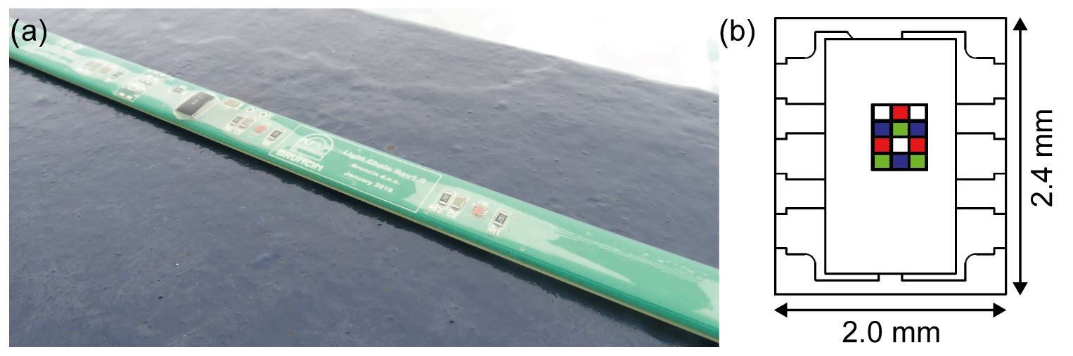
Figure 1(a) A segment of the chain prototype during the calibration procedure. The optical sensors are visible as red-colored components on the circuit board. The black addressing chip controlling the sensors of a particular chain section can be seen in the middle of the picture. (b) Sketch of the arrangement of the different spectral channels on the three-by-four photodiode array of the sensor.
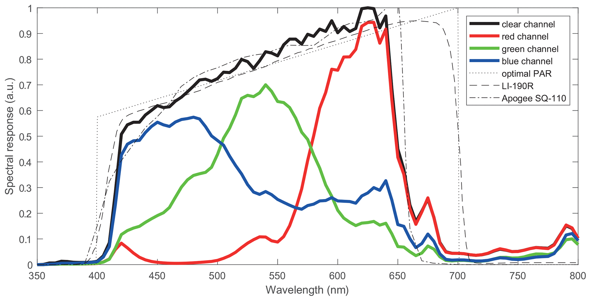
Figure 2Spectral sensitivities of the red, green, blue and clear channel (solid lines). Thin black lines show the spectral sensitivities for different kinds of PAR sensors: theoretical PAR response (dotted line), LI-COR LI-190R sensor (dashed line) and Apogee SQ-110 silicon photodiode sensor (dash dotted line).
As the flat optical sensor is almost directly exposed, it exhibits a good cosine response and thus provides measurements of planar irradiance. The photodiode signals are converted by analog–digital converters on board the chip and transmitted to the board controller using the I2C protocol. The chain consists of eight segments each containing six sensors that are controlled via a I2C interface chip. Thus the entire chain only relies on four continuous electric lines, two for data communication to all sensors and two for 3.3 V power supply. The sensor provides an output in uncalibrated counts that are linearly proportional to the measured irradiance. The digital sensor provides excellent measurement stability and is rated for use at temperatures down to −40 ∘C. It offers a dynamic range of 3 800 000:1 and thus provides precise measurements both under full illumination at the surface and under 2 m thick ice in the Arctic at downwelling planar irradiance fluxes below 0.05 W/m2. In the presented prototype unit, the sensor was always operated at a gain of 1× for highest data quality, but higher gain values of 4×, 16× and 60× can be used to increase low-light sensitivity.
2.3 First deployment
After development and fabrication by Bruncin Observation Systems in spring 2018, the first prototype was deployed during the AO18 expedition of the Swedish research icebreaker Oden (Fig. 3). The icebreaker anchored for 4 weeks at an ice floe in vicinity to the geographic North Pole. On 20 August 2018, the light chain system was deployed as part of a modular ice mass balance and radiation station. Apart from the light chain, the system consisted of three RAMSES-ACC-VIS hyperspectral radiometers (TriOS GmbH, Rastede, Germany) measuring downwelling, reflected and transmitted planar irradiance in the wavelength range of 320–950 nm at 3 nm spectral resolution. The RAMSES sensors and their associated data processing have been described in detail by Nicolaus et al. (2010b). In addition, it comprised a webcam, sensors for snow height, water temperature, water salinity, and a thermistor chain measuring a vertical profile of ice temperature and thermal conductivity. This installation was part of a setup of multiple autonomous measurement systems including a Snow Buoy (MetOcean Telematics, Halifax, Canada), a bio-optical buoy, a Ice Atmosphere Ocean Observing System (IAOOS) buoy with an atmospheric lidar and an ocean profiler (Gascard, 2011), and a time lapse camera.
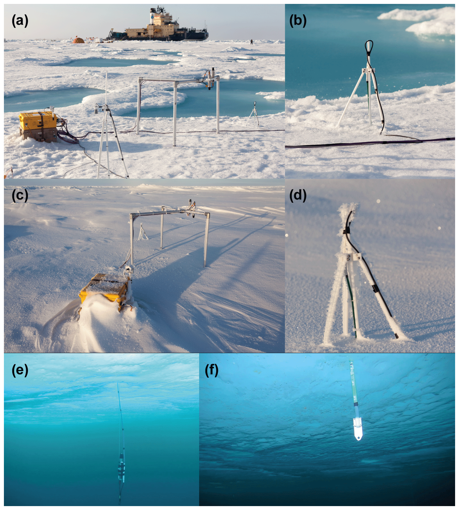
Figure 3(a) Picture of the radiation station setup a few days after deployment on 23 August 2018: from left to right one can see the two cases with electronics, separate batteries and a webcam, the tripod holding a snow height sensor and the thermistor chain, the radiation frame holding the RAMSES radiometers, and the small tripod holding the light chain. (b) Close-up of the light chain. (c, d) The system state on 15 September 2018. (e) Under-ice RAMSES sensor measuring transmitted hyperspectral irradiance. (f) Lowermost portion of the light sensor chain protruding the ice–ocean interface. Note the attached metal weight to keep the chain vertical in the water column.
The light chain was deployed through a 5 cm hole on bare ice of 2.05 m thickness. The topmost part of the hole was backfilled with cuttings and the surface scattering layer restored. The level ice was covered by a 10–15 cm thick surface scattering layer. Backtracking by the ICETrack algorithm (Krumpen et al., 2019) assigned an age of 3 years to this ice, which is in accordance with ice core salinity data (not shown). The light chain was deployed approximately 1.5 m away from a melt pond, which might have influenced the measured in-ice radiation field (Petrich et al., 2012). When the site was left on 15 September 2018, about 5 cm of snow had fallen, reducing overall light transmission.
Two weeks after deployment, on 3 September 2018, one of the control chips on the chain failed, probably due to physical forces during refreezing or in-ice pressure. This failure disabled the fourth section of the chain and heavily influenced readings from section 8. About 10 d later, a similar failure occurred in chain sections 2 and 6. All other chain sections provided useful data, until absolute light levels dropped below 0.05 W/m2 in the beginning of October. Total failure of the system occurred in December 2018, when the entire system ceased data transmission for unknown reasons.
2.4 Calibration
For scientific use, the TCS3472 sensors along the chain have to be cross calibrated. Absolute calibration is generally not necessary, since the data are mainly used as relative measurements between different sensors on the same chain. For different applications, absolute calibration might be necessary. The calibration has to be performed separately for all four spectral bands. To ensure a consistent calibration of the chain, it was strapped flat on the ship's railing with all sensors pointing upwards for several days. To avoid effects of shadowing and different sensor views of the ship's superstructure, we only used data from strongly overcast weather conditions for the calibration. Each channel and all sensors were compared against the average along all chain sensors for each recorded time step. From this, individual calibration coefficients that were applied to each sensor and channel of the entire dataset before further processing were derived. This procedure does not account for calibration uncertainties in between channels. Retrieval of exact spectral ratios between channels would thus require a full absolute radiometric lab calibration of across all sensors and channels. Such a more sophisticated calibration could be performed by the manufacturer in a custom integration sphere before fieldwork, but this would increase system cost dramatically.
2.5 Radiative transfer model
To evaluate the effect of the sideward-looking sensor geometry, we modeled the ice internal radiance field with the radiative transfer model DORT 2002 version 3.0 (Edström, 2005). DORT 2002 is an independent MATLAB implementation of the discrete ordinate radiative transfer model DISORT (Hamre et al., 2004; Laszlo et al., 2016; Stamnes et al., 1988) specifically designed for easy application in highly scattering media. To approximate the ice geometry during the light chain deployment, we used a four-layer model with the following typical inherent optical properties of multiyear ice: a transparent atmosphere with fully isotropic downwelling radiance distribution; a 0.1 m thick surface scattering layer with an absorption coefficient a=0.15 m−1, a scattering coefficient b=250 m−1 and a Henyey–Greenstein phase function with asymmetry parameter g=0.9; a 2 m thick interior ice layer with an absorption coefficient a=0.15 m−1, a scattering coefficient b=25 m−1 and a Henyey–Greenstein phase function (g=0.9); and an underlying ocean with an absorption coefficient of a=0.15 m−1 and a scattering coefficient b=0.1 m−1. These parameters were chosen by values previously used in the literature (Ehn et al., 2008b; Light et al., 2008; Petrich et al., 2012) and adjusted so that they resulted in calculated ice–albedo and transmittance values very similar to our observations. The goal of this modeling analysis is the general evaluation of the sideward-looking sensor orientation and not an exact reproduction of the deployment situation; thus we did not further tune the optical parameters to a perfect fit to the observations.
Downwelling planar, downwelling scalar and sideward planar irradiances were calculated from the resulting radiance distributions using Lebedev quadrature (Katlein et al., 2016; Light et al., 2003).
3.1 Vertical profile of sideward planar irradiance
Figure 4 shows the measured sensor response in the clear channel after along-chain cross calibration. The sensor chain successfully captures the spatiotemporal variation of the in-ice light field from the surface through the ice to the underlying ocean. The dynamic range of the sensor is sufficient to cover the incoming light field as well as the under-ice light field. The expected decay of the light field with increasing depth becomes obvious in the measurements and, except for a few sensor failures, data could be recorded until solar incoming radiation significantly decreased by end of September 2018.
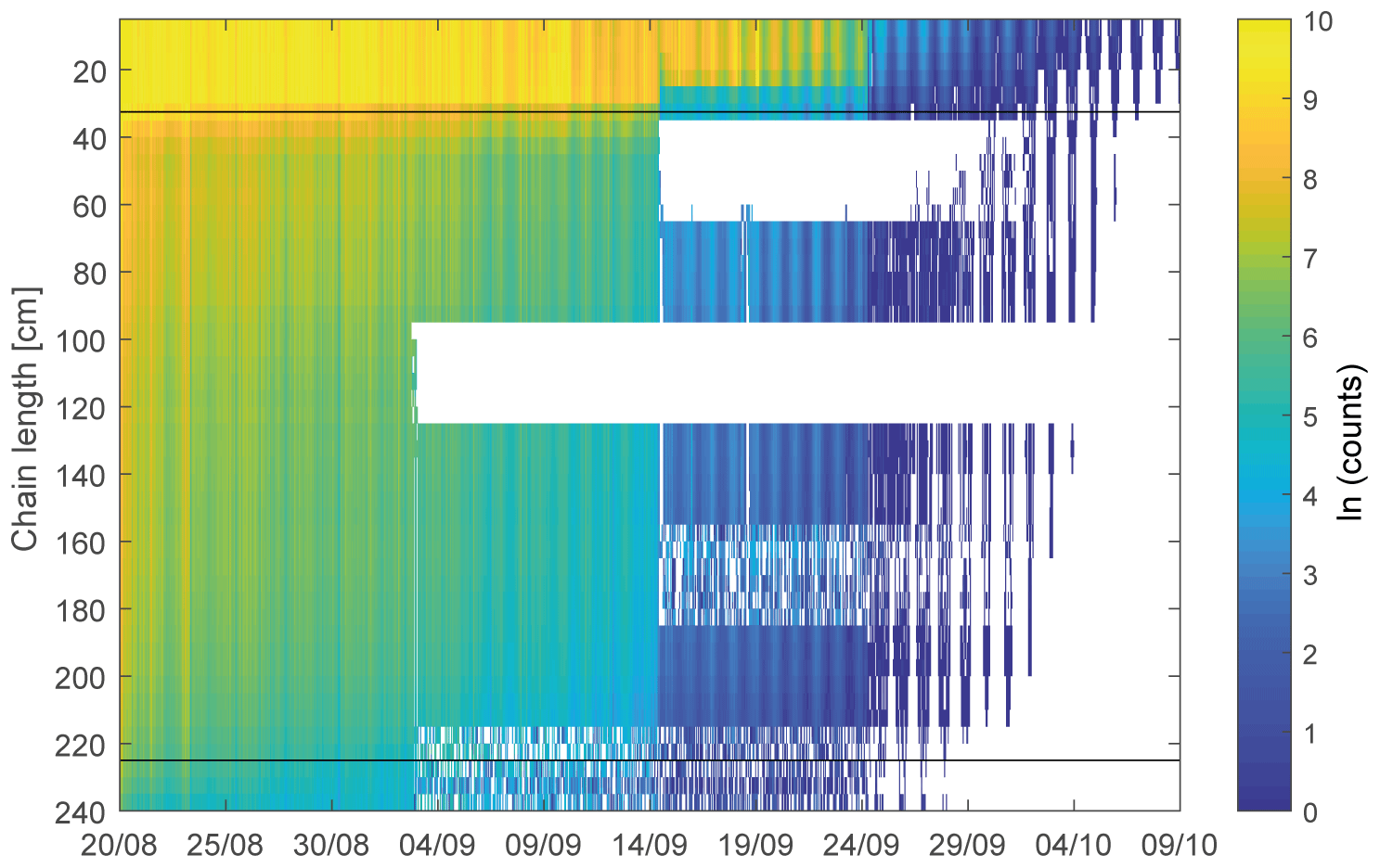
Figure 4Data from the clear channel of the light chain, shown as the natural logarithm of sensor count after cross calibration of chain sensors. Horizontal black lines indicate the air–ice and the ice–ocean interface during deployment of the light chain.
Figure 5 shows sample vertical profiles of sideward planar irradiance along the chain length, and in particular throughout the ice column. The strongest light attenuation is associated with the surface scattering layer and the top 0.2 m of the ice. Below 0.3 m, the decrease becomes more uniform until a depth of approximately 1.5 m. The decrease is linear in the logarithmic plot, which means it closely follows an exponential decay law. This suggests that, in this interior part of the ice, the radiance distribution has reached the asymptotic limit. In this regime, the light attenuation is only dependent on the inherent optical properties of the medium and not on local slab geometry or the incident light field. Also, the radiance distribution is constant with depth, and thus all attenuation coefficients of radiance, downwelling planar irradiance, sideward planar irradiance and scalar irradiance are identical. Beneath 1.5 m, the decay of sideward planar irradiance accelerates, representing increasing loss of photons into the underlying weakly scattering water. This apparent change in light attenuation is associated with the vicinity of an interface, i.e., the underlying ocean, and is not necessarily related to changes in the inherent optical properties of the ice. Under close investigation, the profiles in Fig. 5 exhibit two layers with slightly different optical properties with stronger light attenuation between 0.3–1.0 m than in the underlying layer between 1.0–1.5 m. This is likely due to a different age and thus brine or bubble content of the two respective ice layers. Figure 5a also clearly shows that light in the red channel is attenuated significantly stronger than light in the other spectral channels, but otherwise results for the different channels are very similar. Another notable feature of the profile is an increase between 0.2 and 0.3 m. It could result from locally enhanced scattering, an effect of the sampling hole, an effect of the adjacent pond or refraction at the lower boundary of the scattering layer or the waterline.
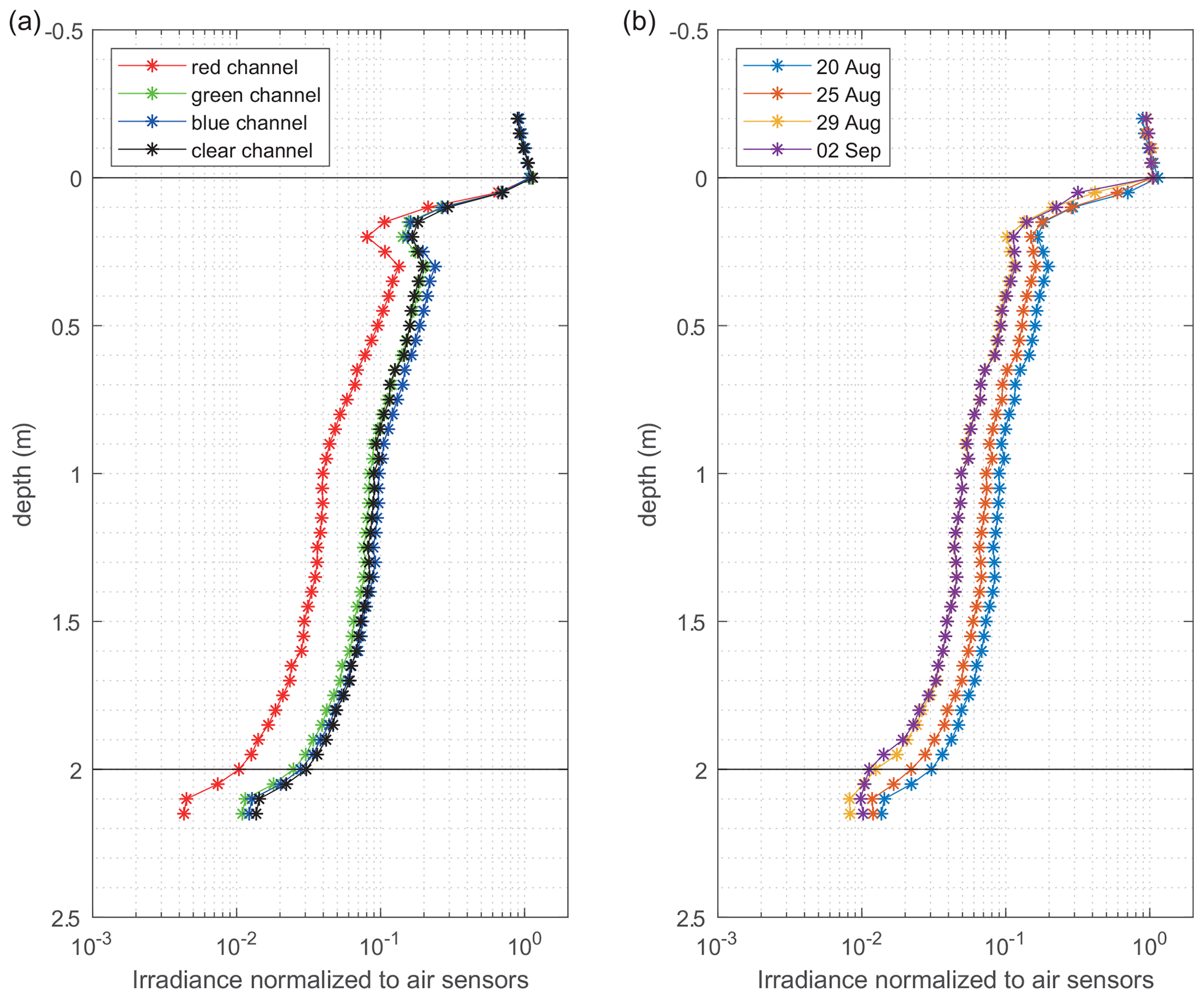
Figure 5Vertical profiles of sideward planar irradiance through sea ice. (a) Irradiance decay in the four spectral channels shortly after deployment on 20 August 2018. (b) Temporally increasing light attenuation for the clear channel from 20 August to 2 September. Black lines indicate the interfaces between air, ice and ocean.
3.2 Diffuse attenuation coefficients
Figure 6 shows the apparent diffuse attenuation coefficients of sideward planar irradiance as derived from neighboring sensor pairs. The vertical diffuse attenuation coefficients κi,j of sideward planar irradiance were derived from pairs of neighboring values of sideward planar irradiance (Ei,Ej) and the distance d between sensors:
Due to remaining calibration uncertainties, as well as the impact of macroscopic variations in the ice structure (e.g., large brine channels), the retrieved coefficients vary a lot between neighboring sensor pairs. However, this variation is consistent over time and thus could be accounted for by vertical smoothing.
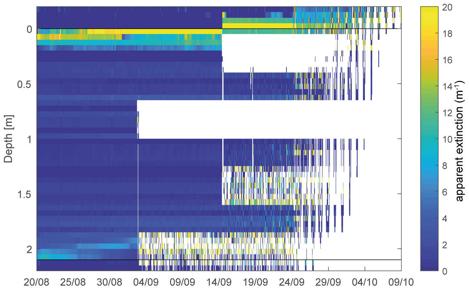
Figure 6Vertical profiles of apparent extinction coefficients calculated from light chain data. Black lines indicate the interfaces between air, ice and ocean during chain deployment.
The highest attenuation coefficients >20 m−1 are associated with the air–ice interface, while they remain typically below 2 m−1 for the ice interior. Towards the ice bottom, apparent attenuation coefficients increase to 4–10 m−1 as the asymptotic regime is passed. This is caused by increasingly strong photon loss through the underside of the ice and not a change in the inherent optical properties of the ice. This layer moves upward with time, likely due to a reducing ice thickness as a result of bottom melt.
3.3 Temporal evolution of ice and snow optical properties
Figure 7 provides a close-up look on the temporal evolution of light attenuation in the first 0.5 m of the chain. Comparing the attenuation data to snow height measurements by acoustic sensors deployed together with the chain, as well as a Snow Buoy deployed in the vicinity of the light chain, shows clearly how an increasing snow cover increases the apparent light attenuation in the sensor pair at the air–ice (snow) interface. After a significant snowfall event on 14 September 2018, the vertical position of the strongly attenuating layer shifted in accordance with the increased snow depth. Due to the strong scattering in the snow and surface scattering layer, radiative losses are highest directly in the uppermost centimeters, where apparent attenuation quickly reaches values above 20 m−1. Spectrally integrated attenuation in the layer directly beneath the surface is largest even when the interface location changes. This high scattering also causes the radiance distribution to quickly reach the asymptotic state, leading to a nearly exponential decay of light within the surface layer (Fig. 5). The vertical sensor spacing of this particular light chain is 5 cm and therefore too coarse to determine snow optical properties precisely, and retrieved values of the uppermost snow layer are thus highly dependent on the actual geometric position of the interface between the two respective surface sensors. The uppermost sensors can also easily be influenced by frost, rime or snow deposited onto the chain by wind as well as local snow accumulations around the sensor chain that do not necessarily represent the overall snow conditions. Such effects are likely causing the significant temporal variation in apparent attenuation coefficients of the top 5 cm, e.g., between 30 August and 14 September.
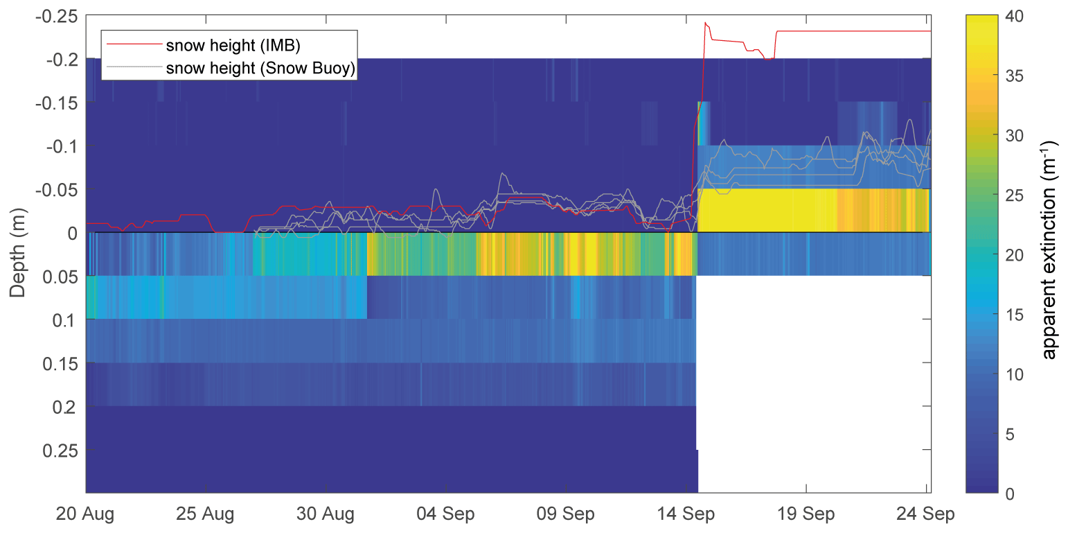
Figure 7Close-up of the vertical profiles of apparent extinction coefficients calculated from light chain data in the uppermost sensor pairs. Snow height measured from the neighboring acoustic pinger of the ice-mass-balance buoy (red) and from the four acoustic pingers of the snow buoy (gray lines). The black line indicates the interfaces between air and ice during chain deployment.
Vertical and temporal profiles of attenuation coefficients for the ice interior are shown in Fig. 8. Averaging the resulting apparent attenuation coefficient for each depth layer reveals a typical structure of light attenuation within sea ice. The topmost 0.15 m is characterized by very high attenuation in the so-called surface scattering layer, consisting of large deteriorating ice grains (Fig. 8a). From 0.4 to 1.8 m depth, the retrieved attenuation coefficients are representative of more homogenous interior sea ice. While local variations in optical properties in the direct vicinity of the sensor cause significant scatter between neighboring depth layers, several regimes of light attenuation are clearly discernable. An upper layer roughly between 0.3 and 1.0 m depth exhibits vertical attenuation coefficients around1.5 m−1, while further below values scatter around 0.5–1.0 m−1. This likely corresponds to different annual growth layers with differences in optical properties of this multiyear ice floe and is consistent with previous observations of light attenuation in interior ice (Light et al., 2008). Below 1.6 m, approximately 0.5 m away from the ice–water interface, derived attenuation values start to increase. This is however not related to a vertical change in the optical properties but to the increasing photon loss through the ice–water interface. As the scattering coefficient of clear Arctic seawater is much lower compared to ice, the number of photons scattered back to the ice by the water is reduced considerably.

Figure 8(a) Time-averaged attenuation coefficients for the first complete set of time series until 14 September for all four channels. (b) Bulk attenuation coefficient averaged over the entire vertical domain. From top to bottom: red, green, blue and clear channel. (c) Ice interior attenuation coefficient for all four channels, determined as the average of attenuation coefficients from 0.35 to 1.8 m depth. (d) Time series of clear-channel attenuation coefficient for different vertical ice layers. The black line equals the black line in panel (c). Sudden changes on 3 September 2020 are caused by partial failure of the sensor chain.
When looking at a time series of vertically averaged (bulk) attenuation coefficients for the entire chain length (Fig. 8b), we observe values increasing from 1.7 to 2.1 m−1 for the green, blue and clear channels. These values are consistent with typical bulk attenuation coefficients used in model parameterizations (Perovich, 1996; Grenfell and Maykut, 1977) and larger-scale estimations of bulk attenuation coefficients during summer (Katlein et al., 2019). Bulk attenuation coefficients for the red channel are slightly higher, increasing from 2.2 to 2.6 m−1 as the absorption coefficient of ice and water is higher in the red part of the spectrum (Grenfell and Perovich, 1981). It remains unclear to us why this prototype shows lower attenuation in the clear channel than the green and blue channels, instead of the expected values between the red and the blue and green channels. This effect did not occur in the deployments during spring 2020 (not described here) and thus seems to be related to either instrument uncertainties or the influence of nearby melt ponds.
While the sensor spacing of 0.05 m is not sufficient to discriminate between different snow layers, it still enables us to also investigate the temporal evolution of optical properties in individual ice layers (Fig. 8c, d). Of particular interest here is the ice interior between 0.3 and 1.8 m, where light attenuation is little affected by boundaries, and the light attenuation coefficient is directly related to the material-inherent optical properties. The retrieved values are in the same order as previous observations, with attenuation coefficients for the clear channel rising from 0.8 to 1.0 m−1 and for the red channel from 1.1 to 1.3 m−1 (Light et al., 2008; Grenfell and Maykut, 1977; Perovich, 1996).
3.4 Interpretation of sideward planar irradiance data
A main factor in the design of the presented light sensor chain is that sensors are oriented sideward in contrast to normal radiation sensors that are usually oriented horizontally. Most autonomous radiation stations measure planar irradiance, as this is an essential quantity for physical processes, describing the directional flux of light energy through a plane (Nicolaus et al., 2010a, b; Wang et al., 2014). For biological applications, scalar irradiance, which describes the non-direction-depending total energy flux through a certain point in space, is however of greater importance (Arrigo et al., 1991; Ehn et al., 2008a; Morel and Smith, 1974). Radiative transfer modeling of the observed ice cover however allows us to derive general relationships between sideward-looking and horizontally oriented irradiance measurements. Figure 9a presents profiles of downwelling planar, scalar and sideward planar irradiance in atmosphere, snow, ice and ocean as simulated using the DORT2002 radiative transfer model (see Sect. 2.5). It is evident that both sideward planar and scalar irradiance exhibit stronger attenuation close to the ice bottom in comparison to planar downwelling irradiance. This is caused by increasing photon loss through the ice–ocean interface. Photons traveling in the downwelling direction – which provide the largest contribution to planar downwelling irradiance – are least affected by the proximity of the ice–ocean interface. Thus attenuation of downwelling planar irradiance closely follows an exponential decrease with depth in a wider vertical range compared to scalar and sideward planar irradiance.
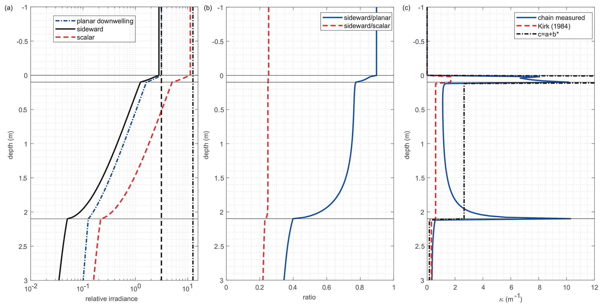
Figure 9(a) Modeled irradiance curves for planar downwelling irradiance (blue dash dotted line), sideward irradiance (black solid line) and total scalar irradiance (red dashed line). Vertical black lines depict the values of π (dashed line) and 4π (dash dotted line), representing the values of planar downwelling and total scalar irradiance, respectively. Horizontal black lines indicate the interfaces between atmosphere, surface scattering layer, ice interior and water. (b) Modeled ratios between sideward and planar downwelling (blue solid line), as well as sideward and total scalar irradiance (red dashed line). (c) Modeled attenuation coefficients as measured by the chain (blue solid line), as well as pseudo-IOP (inherent optical properties) attenuation coefficients derived from model IOP: diffuse attenuation coefficient parameterized according to Kirk (1984) (dashed red line) and the beam attenuation coefficient (dash dotted black line).
The most important conclusion can be reached by comparing ratios of the three irradiance quantities (Fig. 9b). The ratio of sideward to planar irradiance decreases with depth: a ratio of 0.9 applies above sea ice. Values around 0.75 are representative for the asymptotic regime in the ice interior, while a ratio ≤0.4 is found in the underlying water column. For the ratio of sideward to scalar irradiance, we see however that the ratio is close to 0.25 throughout all media. The measured sideward irradiance data can thus easily be converted to total scalar irradiance by multiplication with a factor of 4. Any measurement of sideward planar irradiance within a strongly scattering medium is thus essentially proportional to a measurement of total scalar irradiance. As scalar irradiance is particularly sought after for any studies of biological productivity, this equivalency provides an efficient means to autonomously measure light levels within solid sea ice also with high relevance for such studies. Direct sensing of downwelling planar irradiance would require horizontal sensors and thus a larger geometric footprint and also result in a significant impact of self-shading.
Due to the multiple scattering nature of light transfer in sea ice, the diffuse attenuation coefficients can generally not be directly inferred from the material's inherent optical properties. Comparing modeled attenuation coefficients of sideward planar irradiance with two parameterizations from the field of ocean optics (Kirk, 1984; Mobley, 1994), which are not able to reproduce the observed attenuation profile, clearly indicates this (Fig. 9c). However it is evident that, in the asymptotic regime within the ice interior, the attenuation coefficients are closely linked to the material properties. Additionally, within the asymptotic regime the attenuation coefficients for all three irradiance quantities are identical (Mobley, 1994), so that ice internal attenuation coefficients for downwelling planar irradiance can be derived from the presented measurements of sideward planar irradiance. The asymptotic regime is characterized by the area far enough from medium boundaries, where the angular radiance distribution is invariant with depth. This is quickly reached for the ice interior, in particular due to the overlaying, highly scattering snow and surface layers.
3.5 Comparison to classical hyperspectral setup
To assess the applicability and accuracy of the light sensor chain, we compare sea ice bulk transmittance derived from the chain with measurements from the co-deployed hyperspectral RAMSES radiometer station. Due to the horizontal orientation of the surface sensor, such a derivation is highly sensitive to shadowing and azimuthal effects under clear sky but can be very accurate for the highly isotropic radiance distribution frequently caused by the persistent low cloud cover in the summer Arctic.
Sea ice light transmittance T in the respective spectral channels (RGBC) was derived by averaging sideward planar irradiance values E of the first three sensors (nos. 1, 2, 3) along the chain above the air–ice (snow) interface and the last three sensors (nos. 46, 47, 48) underneath the ice–ocean as . RAMSES hyperspectral radiometer measurements above (Ein(λ)) and below (Etrans(λ)) the ice were folded with the spectral sensitivity c(λ) of the respective bands of the TCS3472 sensor (Fig. 2) to achieve intercomparable results:
A time series of light transmittance for the different spectral channels and both instruments is shown in Fig. 10a. Ice transmittance in the clear channel decreased from 3 % at the start of measurements to <2 % before the failure of the bottommost sensors. Transmittance derived from the light chain generates a time series consistent with the RAMSES measurements. Sea ice transmittance is slightly overestimated in the clear and the blue channel, while the light chain underestimates transmittance in the red and green channel. Overall, the agreement between both setups is striking, with root mean square errors (RMSEs) of 0.003, 0.0048, 0.0036 and 0.0059, respectively, for the red, green, blue and clear channels. A maximum RMSE of 0.59 % transmittance is a particularly good result, given the abovementioned geometric limitations, with a cost reduction by more than a factor of 10.
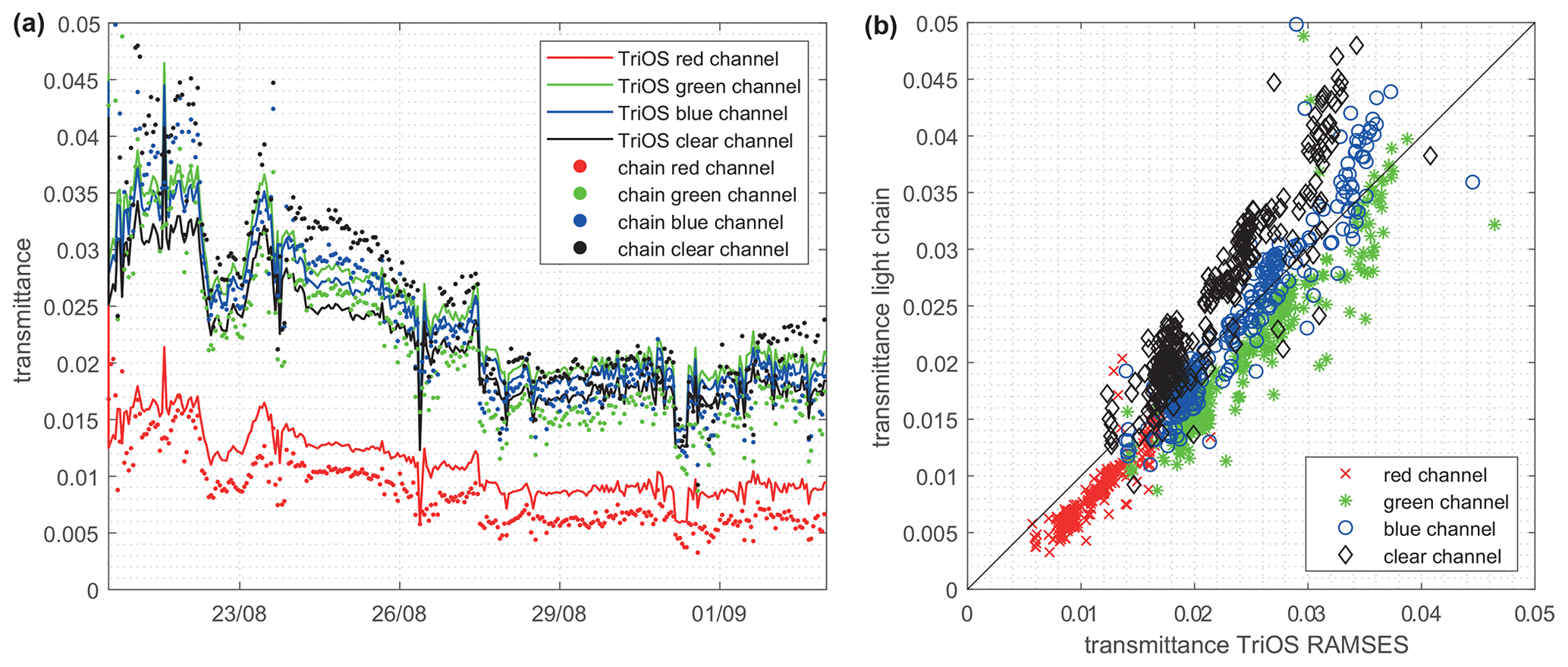
Figure 10(a) Time series of sea ice transmittance in four spectral bands derived from the top- and bottommost chain sensors (dots), as well as from TriOS RAMSES radiometers above and below the ice (solid line). (b) Scatter plot of the dataset showing how close measurements from the light chain agree with high-quality hyperspectral spectroradiometers.
3.6 Spectral signatures
The four spectral bands of the light sensor chain also allow a simple assessment of light color and spectral changes over time. Our first results suggest that there is potential to detect at least transient high concentrations of in-ice algae by this light sensor chain, either in RGB plots or simple band ratios similar to remote sensing algorithms. Unfortunately, a total failure of our buoy in December 2018, far before the first major spring blooms, prevents us from presenting such an analysis here.
To assess the radiometric quality of multispectral light chain data, we also compared RAMSES-measured light spectra with the corresponding chain derived transmittance data for individual days (Fig. 11). A consistent underestimation of chain measurements in the green makes it however difficult to derive a true spectral shape of transmitted light from light chain measurements. This might be caused by either an overall low spectral accuracy of the low-cost sensors or a spectral sensitivity that differs from the one provided by the sensor manufacturer. These issues could certainly be addressed by a more detailed individual spectral calibration of all chain sensors, which in turn would however jeopardize our low-cost approach. High spectral accuracy can be achieved on classical radiation station setups using for example the RAMSES hyperspectral radiometers (Nicolaus et al., 2010b) and thus does not need to be provided by the light sensor chain. The low-cost approach of the light sensor chain however allows for much more widespread deployments, with the potential to yield a much better spatiotemporal resolution of sea-ice-associated light measurements in the Arctic and Antarctic.
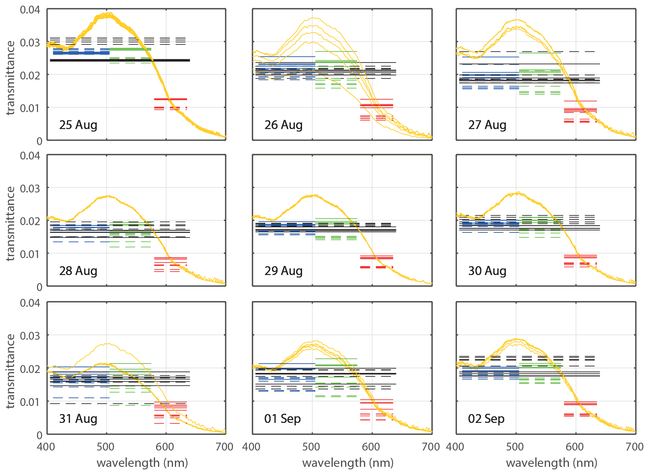
Figure 11Spectral transmittance data of the five measurements centered around solar noon during 9 d of the deployment: transmittance spectra measured by the TriOS RAMSES radiometers (yellow) are overlain by horizontal lines for the four different spectral bands (red, green, blue and clear) reconstructed from TriOS RAMSES spectra (solid lines) and chain measurements (dashed lines).
Apart from shadowing and uncertainties in the calibration and spectral response, the differences in the above comparisons between the light sensor chain and the RAMSES measurements might also arise from the different measured basic irradiance quantities, namely planar and sideward planar/ scalar irradiance, and thus slightly different spectral signatures. For detection of spectrally distinct features, such as ice-algal blooms, spectral attenuation coefficients as well as band ratios are thus more useful than absolute spectral fluxes.
4.1 Implications for radiative transfer modeling
Most autonomous optical measurements in the sea ice environment have been limited to measurements above and below the ice (Nicolaus et al., 2010a; Wang et al., 2014). Detailed investigations show, however, that a vertically resolved measurement provides a better basis for the estimation of light attenuation in sea ice (Light et al., 2008; Ehn et al., 2008a). In our case, the light sensor chain allows for a direct autonomous measurement of the diffuse attenuation coefficient within the ice interior. The equivalency of scalar and planar diffuse attenuation coefficients within the asymptotic regime in the ice interior makes this direct measurement possible. The acquisition of such data is urgently needed as input parameter for simple radiative transfer schemes in large-scale models.
Our results also highlight the strongly non-exponential decay of scalar irradiance in the lowermost 50 cm of the ice cover. This effect is currently mostly unaccounted for in simple exponential radiative transfer parameterizations but reduces light levels at the ice bottom by up to a factor of 2–3. Exponential models of the decay of downwelling planar irradiance have a much wider vertical range of applicability, but also here photon loss in the lower ice portion is currently unaccounted for. A precise measurement of the in-ice diffuse attenuation coefficient however allows at least for accurate tuning of exponential parameterizations. This is of great advantage, as this parameter cannot be easily derived from the inherent optical properties of the ice. To test the accuracy of such a measurement-supported exponential parameterization, we compare the sea ice transmittance time series acquired by the RAMSES hyperspectral setup to a simple exponential parameterization, where sea ice light transmittance T is parameterized as a function of ice thickness z, ice surface albedo α as measured by RAMSES and the chain-derived ice-interior diffuse attenuation coefficient κchain:
The resulting time series (Fig. 12) is in close agreement with the light transmittance as measured by the RAMSES setup. Measured albedo values were reduced by 0.05 to avoid albedo values larger than 1.
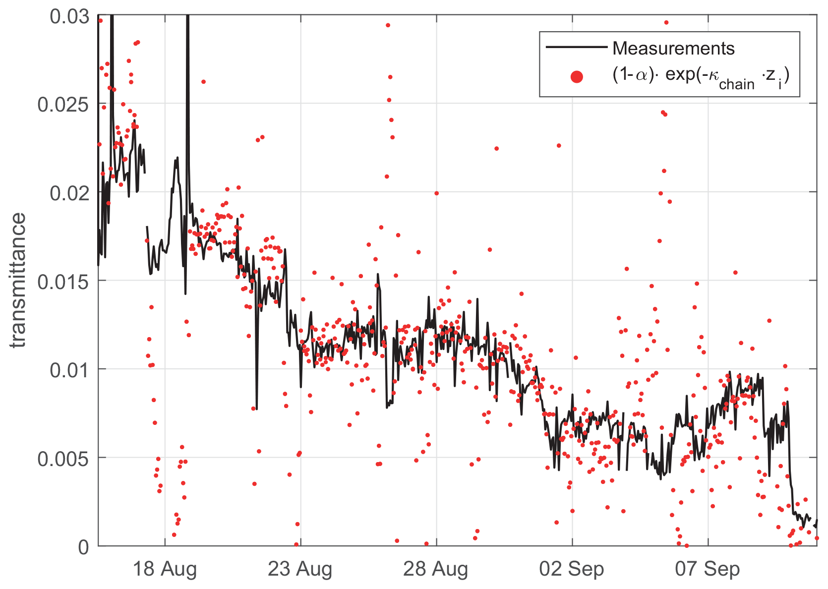
Figure 12Time series of sea ice light transmittance as observed by the traditional RAMSES setup (black line) and a simple light chain data assisted exponential parameterization (red points) based on observed albedo and diffuse attenuation coefficients. The high scatter of the parameterizations is caused by scatter in the albedo data measured by the RAMSES setup.
4.2 Limitations
As mentioned above (Sects. 2 and 3.1), the radiometric quality of the sensors after initial field calibration is sufficient for studies of the light field in all four spectral channels. While the clear channel is very close in spectral characteristics to commercially available sensors for photosynthetically active radiation (PAR), it cuts off at 650nm instead of 700 nm (Fig. 2). This does not have a huge impact on flux measurements under sea ice but slightly overestimates PAR transmittance.
The absolute spectral accuracy of the presented system is unfortunately limited, as shown in Sect. 3.6. Part of this uncertainty could also originate from the poorly characterized spectral transmittance of the heat shrink covering the sensors. Manufacturing differences and material aging make it difficult to precisely account for spectral transmittance of the heat shrink. A lab experiment revealed the highest heat shrink transmittance for the blue channel, with 3 % relative reduction in the red, 6 % in the green and 21 % in the clear channel. However, it is still highly useful for the observation of temporally changing band ratios. Similarly, this low-cost system does not provide a true measurement of sea ice transmittance of planar irradiance, as the sideward-looking sensors can introduce artifacts due to azimuthal orientation and self-shadowing.
The geometry of the sideward-looking setup poses some challenge for the interpretation of data from the light sensor chain. This was however partly solved by the equivalency of sideward planar irradiance and total scalar irradiance, as total scalar irradiance is a primary target for biological studies. Total scalar irradiance can be converted back to planar irradiance in the case of a known mean cosine of the light field. Our model results together with recent other works (Matthes et al., 2019; Katlein et al., 2014b) can provide guidance on the appropriate choice of mean cosine in and underneath sea ice. However these equivalencies can of course only be valid for undirected diffuse and azimuthally homogenous light fields. While such diffuse light fields are prevalent in most in- and under-ice scenarios, more directional light fields can occur during cloud-free conditions particularly above the ice surface, within the first layers and if a surface scattering layer is absent.
The detection limit of the sensor is sufficiently low to provide reliable optical data at absolute irradiances down to less than 0.05 W/m2. This enables the light chain to detect light levels under 2 m thick Arctic ice in autumn, e.g., even when the sun is already a few degrees below the horizon. This dynamic range can be further increased with more advanced settings on sensor gain and exposure.
The impact of the deployment hole itself and its refreezing process is however of even less importance than for traditional thermistor string observations. The sideward planar irradiance sensors observe scattered photons from a larger footprint and are thus not strongly influenced, e.g., by the distance of the sensor to the hole wall. In turn, larger brine channels, or air inclusions can locally alter the light field, leading to the observed scatter in the retrieved vertical attenuation coefficients.
While the sensor spacing of 5 cm seems to excellently resolve the vertical decay of light within sea ice, this vertical resolution is not high enough to decipher detailed optical properties of the snow pack and surface scattering layer. In addition, application of appropriate but difficult to determine immersion factors would allow us to correct the chain data for differences in refractive index across the different media. As these interfaces move over time, the precise detection of the vertical position of interfaces between water, ice, snow and air is limited. These measurements can however be easily obtained from co-deployed, e.g., sonic ice and snow thickness sounders.
4.3 Recommendations for future deployments
For future deployments of the system, we want to stress the importance of sensor calibration before deployment. This can be simply done by stretching the chain out, e.g., along the ships railing, and fixing it in a place with comparable lighting conditions all along the chain. To achieve the best calibration accuracy, this exercise should be performed for several days and in the best case during foggy weather with a close-to-isotropic light field. If this step is omitted, radiometric accuracy of the light sensor chain is much reduced.
Also, it should be noted that sufficient information about the ice interior attenuation coefficient – and thus the ice inherent optical properties – can only be achieved if the light sensor chain is deployed on sufficiently thick ice, where the asymptotic limit is reached. Our data suggest that this condition will not be satisfied for sea ice with a thickness below 1 m. While the sensors will still provide reliable radiometric measurements, a detailed interpretation of attenuation coefficients then needs to be supported by explicit radiative transfer modeling.
A great opportunity will be the co-deployment of light sensor chains with classical thermistor-chain buoys. This will allow for a closer investigation of the dependency of ice optical properties and the thermodynamic state of the ice. It might also provide crucial input for structural optical models and radiative transfer parameterizations. In particular, the low unit cost enables more frequent autonomous deployment of optical sensors to cover some aspects of spatial variability. A combination of light chain deployment with ice core analysis of temperature, salinity and texture close to the deployment site will further improve the interpretation of the optical data.
For the next deployments, an upgraded version of the sensor chain will provide more physical strength to avoid partial chain failures as observed in this first deployment. Furthermore, the light sensor chain will be outfitted with a standard serial interface enabling easy integration in almost any data logging system.
To increase the scientific use of the sensor chain especially during the dark period of the year, the chain can be upgraded to contain LED lighting elements. This would allow for active sensing of the ice optical properties also in the winter. If the spatial resolution of optical sensors along the chain is increased, this chain could also be used for diffuse reflectance spectroscopy (Kim and Wilson, 2011), where the inherent optical properties of sea ice can be determined by active measurement of the point spread function in sea ice (Maffione et al., 1998; Voss et al., 1992).
We deployed and evaluated a first prototype of an in-ice light sensor chain, designed on the basis of previously developed digital thermistor chains. With only minor sensor failures, the device acquired optical data throughout the autumn of 2018 in the vicinity of the geographic North Pole. Overall we could show that this newly developed sensor chain is able to provide valuable autonomous measurements of the light field within sea ice. The four-channel multispectral sensors embedded in the chain allow for the measurement of a vertical profile of PAR total scalar irradiance, as well as retrieval of multispectral diffuse attenuation coefficients particularly in the ice interior. The equivalency of total scalar and sideward planar irradiance significantly helps the interpretation of the acquired measurements. Measurements within the asymptotic regime in the ice interior allow a more direct relation of optical measurements to the inherent optical properties of sea ice than traditional measurements above and below the sea ice. In addition, the low cost factor of the presented system will allow for more frequent deployments, which will enable us to achieve a much better spatial and temporal coverage of ice-associated light data and help to better understand in particular the spatial variability in sea ice optical properties.
Data of the presented system are publicly available at https://www.meereisportal.de/en/ (last access: 11 January 2021) under the buoy name 2018R4 and can be retrieved at https://data.meereisportal.de/gallery/index_new.php?active-tab1=method&buoytype=RB®ion=all&buoystate=all&expedition=Oden_AO18&buoynode=all&submit3=Anzeigen&lang=de_DE&active-tab2=buoy (Grosfeld et al., 2016).
CK had the idea of a digital light sensor chain, wrote the first draft of the manuscript, and processed and evaluated the light chain data. LV and his team built the prototype unit in close collaboration with MH and CK. MH and CK deployed the instrument in the field. SLG and CK performed the radiative transfer modeling of the sideward irradiance. All authors contributed to the editing of the manuscript.
The authors declare that they have no conflict of interest.
Development and deployment of the unit, as well as the positions of Christian Katlein and Mario Hoppmann, were funded by the Helmholtz Infrastructure Initiative Frontiers in Arctic marine Monitoring (FRAM) and the Alfred-Wegener-Institut, Helmholtz-Zentrum für Polar- und Meeresforschung. Scientific data evaluation and writing of the manuscript was supported by a Sentinel North Postdoctoral Research Fellowship to Christian Katlein and the Takuvik Joint International Laboratory (Université Laval and CNRS). This work represents a contribution to the Diatom ARCTIC project (NE/R012849/1; 03F0810A), part of the Changing Arctic Ocean program, jointly funded by the UKRI Natural Environment Research Council (NERC) and the German Federal Ministry of Education and Research (BMBF).
Deployment of the system and participation in the AO18 expedition of the Swedish icebreaker Oden was facilitated by the Swedish Polar Research Secretariat (SPRS). We want to thank in particular Philipp Anhaus and Matthieu Labaste for field assistance, as well as Anja Nicolaus and Marcel Nicolaus for administrative support around the buoy deployment.
This research has been supported by the Alfred Wegener Institute, Helmholtz Centre for Polar and Marine Research, the Bundesministerium für Bildung und Forschung (grant no. 03F0810A), and the Polarforskningssekretariatet (grant no. AO18).
The article processing charges for this open-access
publication were covered by a Research
Centre of the Helmholtz Association.
This paper was edited by John Yackel and reviewed by two anonymous referees.
Arrigo, K. R., Sullivan, C. W., and Kremer, J. N.: A biooptical model of Antarctic sea ice, J. Geophys. Res.-Oceans, 96, 10581–10592, https://doi.org/10.1029/91jc00455, 1991.
Assmy, P., Fernández-Méndez, M., Duarte, P., Meyer, A., Randelhoff, A., Mundy, C. J., Olsen, L. M., Kauko, H. M., Bailey, A., and Chierici, M.: Leads in Arctic pack ice enable early phytoplankton blooms below snow-covered sea ice, Sci. Rep.-UK, 7, 40850, https://doi.org/10.1038/srep40850, 2017.
Curry, J. A., Schramm, J. L., and Ebert, E. E.: Sea Ice-Albedo Climate Feedback Mechanism, J. Climate, 8, 240–247, https://doi.org/10.1175/1520-0442(1995)008<0240:SIACFM>2.0.CO;2, 1995.
Edström, P.: A Fast and Stable Solution Method for the Radiative Transfer Problem, SIAM Rev., 47, 447–468, https://doi.org/10.1137/s0036144503438718, 2005.
Ehn, J. K., Mundy, C. J., and Barber, D. G.: Bio-optical and structural properties inferred from irradiance measurements within the bottommost layers in an Arctic landfast sea ice cover, J. Geophys. Res.-Oceans, 113, C03S03, https://doi.org/10.1029/2007JC004194, 2008a.
Ehn, J. K., Papakyriakou, T. N., and Barber, D. G.: Inference of optical properties from radiation profiles within melting landfast sea ice, J. Geophys. Res.-Oceans, 113, https://doi.org/10.1029/2007jc004656, 2008b.
Ehn, J. K. and Mundy, C. J.: Assessment of light absorption within highly scattering bottom sea ice from under-ice light measurements: Implications for Arctic ice algae primary production, Limnol. Oceanogr., 58, 893–902, https://doi.org/10.4319/lo.2013.58.3.0893, 2013.
Eicken, H. and Salganek, M.: Field Techniques for Sea-Ice Research, University of Alaska Press, Fairbanks, AK, USA, 2010.
Gascard, J. C.: Steps Toward an Integrated Arctic Ocean Observational System, Oceanography, 24, 174–175, https://doi.org/10.5670/oceanog.2011.69, 2011.
Grenfell, T. C. and Hedrick, D.: Scattering of visible and near infrared radiation by NaCl ice and glacier ice, Cold Reg. Sci. Tech., 8, 119–127, https://doi.org/10.1016/0165-232x(83)90003-4, 1983.
Grenfell, T. C. and Maykut, G. A.: The optical properties of ice and snow in the arctic basin, J. Glaciol., 18, 445–463, 1977.
Grenfell, T. C. and Perovich, D. K.: Radiation absorption coefficients of polycrystalline ice from 400–1400nm, J. Geophys. Res.-Oceans, 86, 7447–7450, https://doi.org/10.1029/JC086iC08p07447, 1981.
Grenfell, T. C., Light, B., and Perovich, D. K.: Spectral transmission and implications for the partitioning of shortwave radiation in arctic sea ice, Ann. Glaciol., 44, 1–6, 2006.
Grosfeld, K., Treffeisen, R., Asseng, J., Bartsch, A., Bräuer, B., Fritzsch, B., Gerdes, R., Hendricks, S., Hiller, W., Heygster, G., Krumpen, T., Lemke, P., Melsheimer, C., Nicolaus, M., Ricker, R., and Weigelt, M.: Online sea-ice knowledge and data platform <www.meereisportal.de>, Polarforschung, Bremerhaven, Alfred Wegener Institute for Polar and Marine Research & German Society of Polar Research, 85, 143–155, https://doi.org/10.2312/polfor.2016.011, 2016 (data available at: https://data.meereisportal.de/gallery/index_new.php?active-tab1=method&buoytype=RB®ion=all&buoystate=all&expedition=Oden_AO18&buoynode=all&submit3=Anzeigen&lang=de_DE&active-tab2=buoy, last access: 11 January 2021).
Haas, C., Pfaffling, A., Hendricks, S., Rabenstein, L., Etienne, J.-L., and Rigor, I.: Reduced ice thickness in Arctic Transpolar Drift favors rapid ice retreat, Geophys. Res. Lett., 35, L17501, https://doi.org/10.1029/2008gl034457, 2008.
Hamre, B., Winther, J. G., Gerland, S., Stamnes, J. J., and Stamnes, K.: Modeled and measured optical transmittance of snow-covered first-year sea ice in Kongsfjorden, Svalbard, J. Geophys. Res.-Oceans, 109, https://doi.org/10.1029/2003jc001926, 2004.
Hoppmann, M., Nicolaus, M., Hunkeler, P. A., Heil, P., Behrens, L.-K., König-Langlo, G., and Gerdes, R.: Seasonal evolution of an ice-shelf influenced fast-ice regime, derived from an autonomous thermistor chain, J. Geophys. Res.-Oceans, 120, 1703–1724, https://doi.org/10.1002/2014jc010327, 2015.
Jackson, K., Wilkinson, J., Maksym, T., Meldrum, D., Beckers, J., Haas, C., and Mackenzie, D.: A Novel and Low-Cost Sea Ice Mass Balance Buoy, J. Atmos. Ocean. Tech., 30, 2676–2688, https://doi.org/10.1175/jtech-d-13-00058.1, 2013.
Katlein, C., Fernández-Méndez, M., Wenzhöfer, F., and Nicolaus, M.: Distribution of algal aggregates under summer sea ice in the Central Arctic, Polar Biol., 38, 1–13, https://doi.org/10.1007/s00300-014-1634-3, 2014a.
Katlein, C., Nicolaus, M., and Petrich, C.: The anisotropic scattering coefficient of sea ice, J. Geophys. Res.-Oceans, 119, 842–855, https://doi.org/10.1002/2013JC009502, 2014b.
Katlein, C., Arndt, S., Nicolaus, M., Perovich, D. K., Jakuba, M. V., Suman, S., Elliott, S., Whitcomb, L. L., McFarland, C. J., Gerdes, R., Boetius, A., and German, C. R.: Influence of ice thickness and surface properties on light transmission through Arctic sea ice, J. Geophys. Res.-Oceans, 120, 5932–5944, https://doi.org/10.1002/2015JC010914, 2015.
Katlein, C., Perovich, D. K., and Nicolaus, M.: Geometric Effects of an Inhomogeneous Sea Ice Cover on the under Ice Light Field, Front. Earth Sci., 4, 6, https://doi.org/10.3389/feart.2016.00006, 2016.
Katlein, C., Schiller, M., Belter, H. J., Coppolaro, V., Wenslandt, D., and Nicolaus, M.: A New Remotely Operated Sensor Platform for Interdisciplinary Observations under Sea Ice, Front. Marine Sci., 4, 281, https://doi.org/10.3389/fmars.2017.00281, 2017.
Katlein, C., Arndt, S., Belter, H. J., Castellani, G., and Nicolaus, M.: Seasonal Evolution of Light Transmission Distributions Through Arctic Sea Ice, J. Geophys. Res.-Oceans, 124, 5418–5435, https://doi.org/10.1029/2018JC014833, 2019.
Kim, A. and Wilson, B. C.: Measurement of Ex Vivo and In Vivo Tissue Optical Properties: Methods and Theories, in: Optical-Thermal Response of Laser-Irradiated Tissue, edited by: Welch, A. J. and van Gemert, M. J. C., Springer, Dordrecht, Netherlands, 267–319, 2011.
Kirk, J. T. O.: Dependence of relationship between inherent and apparent optical properties of water on solar altitude, Limnol. Oceanogr., 29, 350–356, https://doi.org/10.4319/lo.1984.29.2.0350, 1984.
Krumpen, T., Belter, H. J., Boetius, A., Damm, E., Haas, C., Hendricks, S., Nicolaus, M., Nöthig, E.-M., Paul, S., Peeken, I., Ricker, R., and Stein, R.: Arctic warming interrupts the Transpolar Drift and affects long-range transport of sea ice and ice-rafted matter, Sci. Rep.-UK, 9, 5459, https://doi.org/10.1038/s41598-019-41456-y, 2019.
Lange, B. A., Katlein, C., Nicolaus, M., Peeken, I., and Flores, H.: Sea ice algae chlorophyll a concentrations derived from under-ice spectral radiation profiling platforms, J. Geophys. Res.-Oceans, 121, 8511–8534, https://doi.org/10.1002/2016JC011991, 2016.
Laszlo, I., Stamnes, K., Wiscombe, W., and Tsay, S.-C.: The Discrete Ordinate Algorithm, DISORT for Radiative Transfer, in: Light Scattering Reviews, edited by: Kokhanovsky, A., Volume 11, Springer Praxis Books, Springer, Berlin, Heidelberg, https://doi.org/10.1007/978-3-662-49538-4_1, 2016.
Leu, E., Wiktor, J., Soreide, J. E., Berge, J., and Falk-Petersen, S.: Increased irradiance reduces food quality of sea ice algae, Mar. Ecol. Prog. Ser., 411, 49–60, https://doi.org/10.3354/meps08647, 2010.
Light, B., Maykut, G. A., and Grenfell, T. C.: A two-dimensional Monte Carlo model of radiative transfer in sea ice, J. Geophys. Res.-Oceans, 108, https://doi.org/10.1029/2002jc001513, 2003.
Light, B., Grenfell, T. C., and Perovich, D. K.: Transmission and absorption of solar radiation by Arctic sea ice during the melt season, J. Geophys. Res.-Oceans, 113, https://doi.org/10.1029/2006jc003977, 2008.
Light, B., Perovich, D. K., Webster, M. A., Polashenski, C., and Dadic, R.: Optical properties of melting first-year Arctic sea ice, J. Geophys. Res.-Oceans, 120, 7657–7675, https://doi.org/10.1002/2015JC011163, 2015.
Maffione, R. A., Voss, J. M., and Mobley, C. D.: Theory and measurements of the complete beam spread function of sea ice, Limnol. Oceanogr., 43, 34–43, https://doi.org/10.4319/lo.1998.43.1.0034, 1998.
Matthes, L. C., Ehn, J. K., Girard, S. L., Pogorzelec, N. M., Babin, M., and Mundy, C. J.: Average cosine coefficient and spectral distribution of the light field under sea ice: Implications for primary production, Elementa: Science of the Anthropocene, 7, 25, https://doi.org/10.1525/elementa.363, 2019.
Mobley, C. D.: Light and water: radiative transfer in natural waters, Academic Press, San Diego, CA, USA, 1994.
Morel, A. and Smith, R. C.: Relation Between Total Quanta and Total Energy for Aquatic Photosynthesis, Limnol. Oceanogr., 19, 591–600, 1974.
Mundy, C. J., Ehn, J. K., Barber, D. G., and Michel, C.: Influence of snow cover and algae on the spectral dependence of transmitted irradiance through Arctic landfast first-year sea ice, J. Geophys. Res.-Oceans, 112, https://doi.org/10.1029/2006jc003683, 2007.
Nicolaus, M. and Katlein, C.: Mapping radiation transfer through sea ice using a remotely operated vehicle (ROV), The Cryosphere, 7, 763–777, https://doi.org/10.5194/tc-7-763-2013, 2013.
Nicolaus, M., Gerland, S., Hudson, S. R., Hanson, S., Haapala, J., and Perovich, D. K.: Seasonality of spectral albedo and transmittance as observed in the Arctic Transpolar Drift in 2007, J. Geophys. Res.-Oceans, 115, https://doi.org/10.1029/2009jc006074, 2010a.
Nicolaus, M., Hudson, S. R., Gerland, S., and Munderloh, K.: A modern concept for autonomous and continuous measurements of spectral albedo and transmittance of sea ice, Cold Reg. Sci. Tech., 62, 14–28, https://doi.org/10.1016/j.coldregions.2010.03.001, 2010b.
Pegau, W. S. and Zaneveld, J. R. V.: Field measurements of in-ice radiance, Cold Reg. Sci. Tech., 31, 33–46, https://doi.org/10.1016/s0165-232x(00)00004-5, 2000.
Perovich, D. K.: Theoretical estimates of light reflection and transmission by spatially complex and temporally varying sea ice covers, J. Geophys. Res.-Oceans, 95, 9557–9567, https://doi.org/10.1029/JC095iC06p09557, 1990.
Perovich, D. K.: The optical properties of sea ice, CRREL, Hanover, NH, USA, 1996.
Perovich, D. K. and Richter-Menge, J. A.: From points to Poles: extrapolating point measurements of sea-ice mass balance, Ann. Glaciol., 44, 188–192, https://doi.org/10.3189/172756406781811204, 2006.
Perovich, D. K., Longacre, J., Barber, D. G., Maffione, R. A., Cota, G. F., Mobley, C. D., Gow, A. J., Onstott, R. G., Grenfell, T. C., Pegau, W. S., Landry, M., and Roesler, C. S.: Field observations of the electromagnetic properties of first-year sea ice, IEEE Geosci. Remote S., 36, 1705–1715, https://doi.org/10.1109/36.718639, 1998.
Perovich, D. K., Light, B., Eicken, H., Jones, K. F., Runciman, K., and Nghiem, S. V.: Increasing solar heating of the Arctic Ocean and adjacent seas, 1979–2005: Attribution and role in the ice-albedo feedback, Geophys. Res. Lett., 34, https://doi.org/10.1029/2007gl031480, 2007.
Petrich, C., Nicolaus, M., and Gradinger, R.: Sensitivity of the light field under sea ice to spatially inhomogeneous optical properties and incident light assessed with three-dimensional Monte Carlo radiative transfer simulations, Cold Reg. Sci. Tech., 73, 1–11, https://doi.org/10.1016/j.coldregions.2011.12.004, 2012.
Planck, C. J., Whitlock, J., Polashenski, C., and Perovich, D.: The evolution of the seasonal ice mass balance buoy, Cold Reg. Sci. Tech., 165, 102792, https://doi.org/10.1016/j.coldregions.2019.102792, 2019.
Renner, A. H. H., Gerland, S., Haas, C., Spreen, G., Beckers, J. F., Hansen, E., Nicolaus, M., and Goodwin, H.: Evidence of Arctic sea ice thinning from direct observations, Geophys. Res. Lett., 41, 5029–5036, https://doi.org/10.1002/2014gl060369, 2014.
Richter-Menge, J. A., Perovich, D. K., Elder, B. C., Claffey, K., Rigor, I., and Ortmeyer, M.: Ice mass-balance buoys: a tool for measuring and attributing changes in the thickness of the Arctic sea-ice cover, Ann. Glaciol., 44, 205–210, https://doi.org/10.3189/172756406781811727, 2006.
Serreze, M. C., Holland, M. M., and Stroeve, J.: Perspectives on the Arctic's Shrinking Sea-Ice Cover, Science, 315, 1533–1536, https://doi.org/10.1126/science.1139426, 2007.
Stamnes, K., Tsay, S. C., Wiscombe, W., and Jayaweera, K.: Numerically stable algorithm for discrete-ordinate-method radiative transfer in multiple scattering and emitting layered media, Appl. Optics, 27, 2502–2509, https://doi.org/10.1364/AO.27.002502, 1988.
Steele, M., Zhang, J., and Ermold, W.: Mechanisms of summertime upper Arctic Ocean warming and the effect on sea ice melt, J. Geophys. Res.-Oceans, 115, https://doi.org/10.1029/2009jc005849, 2010.
Stroeve, J. C., Serreze, M. C., Holland, M. M., Kay, J. E., Malanik, J., and Barrett, A. P.: The Arctic's rapidly shrinking sea ice cover: a research synthesis, Climatic Change, 110, 1005–1027, https://doi.org/10.1007/s10584-011-0101-1, 2012.
Voss, J. M., Honey, R. C., Gilbert, G. D., and Buntzen, R. R.: Measuring the point-spread function of sea ice in situ, San Diego, CA, USA, 517–526, available at: https://www.spiedigitallibrary.org/conference-proceedings-of-spie/1750/0000/Measuring-the-point-spread-function-of-sea-ice-in-situ/10.1117/12.140682.short?SSO=1 (last access: 11 January 2021), 1992.
Wang, C., Granskog, M. A., Gerland, S., Hudson, S. R., Perovich, D. K., Nicolaus, M., Ivan Karlsen, T., Fossan, K., and Bratrein, M.: Autonomous observations of solar energy partitioning in first-year sea ice in the Arctic Basin, J. Geophys. Res.-Oceans, 119, 2066–2080, https://doi.org/10.1002/2013JC009459, 2014.
Xu, Z., Yang, Y., Sun, Z., Li, Z., Cao, W., and Ye, H.: In situ measurement of the solar radiance distribution within sea ice in Liaodong Bay, China, Cold Reg. Sci. Tech., 71, 23–33, https://doi.org/10.1016/j.coldregions.2011.10.005, 2012.
Zhao, J. P., Li, T., Barber, D., Ren, J. P., Pucko, M., Li, S. J., and Li, X.: Attenuation of lateral propagating light in sea ice measured with an artificial lamp in winter Arctic, Cold Reg. Sci. Tech., 61, 6–12, https://doi.org/10.1016/j.coldregions.2009.12.006, 2010.