the Creative Commons Attribution 4.0 License.
the Creative Commons Attribution 4.0 License.
 | 21 Dec 2020
Numerical modelling of permafrost spring discharge and open-system pingo formation induced by basal permafrost aggradation
Andrew Jonathan Hodson
Søren Jessen
Victor Bense
Kim Senger
In the high Arctic valley of Adventdalen, Svalbard, sub-permafrost groundwater feeds several pingo springs distributed along the valley axis. The driving mechanism for groundwater discharge and associated pingo formation is enigmatic because wet-based glaciers are not present in the adjacent highlands and the presence of continuous permafrost seems to preclude recharge of the sub-permafrost groundwater system by either a subglacial source or a precipitation surplus. Since the pingo springs enable methane that has accumulated underneath the permafrost to escape directly to the atmosphere, our limited understanding of the groundwater system brings significant uncertainty to predictions of how methane emissions will respond to changing climate. We address this problem with a new conceptual model for open-system pingo formation wherein pingo growth is sustained by sub-permafrost pressure effects, as related to the expansion of water upon freezing, during millennial-scale basal permafrost aggradation. We test the viability of this mechanism for generating groundwater flow with decoupled heat (one-dimensional transient) and groundwater (three-dimensional steady state) transport modelling experiments. Our results suggest that the conceptual model represents a feasible mechanism for the formation of open-system pingos in lower Adventdalen and elsewhere. We also explore the potential for additional pressurisation and find that methane production and methane clathrate formation and dissolution deserve particular attention on account of their likely effects upon the hydraulic pressure. Our model simulations also suggest that the generally low-permeability hydrogeological units cause groundwater residence times to exceed the duration of the Holocene. The likelihood of such pre-Holocene groundwater ages is supported by the geochemistry of the pingo springs which demonstrates an unexpected seaward freshening of groundwater potentially caused by a palaeo-subglacial meltwater “wedge” from the Weichselian. Whereas permafrost thickness (and age) progressively increases inland, accordingly, the sub-permafrost meltwater wedge thins, and less unfrozen freshwater is available for mixing. Our observations imply that millennial-scale permafrost aggradation deserves more attention as a possible driver of sustained flow of sub-permafrost groundwater and methane to the surface because, although the hydrological system in Adventdalen at first appears unusual, it is likely that similar systems have developed in other uplifted valleys throughout the Arctic.
- Article
(7788 KB) - Full-text XML
- Companion paper
-
Supplement
(882 KB) - BibTeX
- EndNote


Sub-permafrost groundwater systems are highly inaccessible, and so their investigation usually relies on sparse data (van der Ploeg et al., 2012). However, cold regions increasingly become hydrogeologically active after surface warming and associated permafrost degradation. This implies, for example, an increased outflow of deeper groundwater to rivers and lakes (Bense et al., 2012), increased rates of biogeochemical processes (Grosse et al., 2016), and potentially increased fluxes of methane or other compounds into the surface environment and atmosphere (Schuster et al., 2018). The surface discharge of sub-permafrost groundwater is currently exemplified by springs in the high Arctic (Andersen et al., 2002; Grasby et al., 2012; Haldorsen et al., 1996; Williams, 1970). If conditions are favourable, spring outflow may instead freeze below the active layer and initiate the growth of an ice-cored hill or pingo. By definition, this would be classified as an open-system pingo because of the open connection to the sub-permafrost groundwater (Liestøl, 1996). Considerable methane stocks may exist below continuous permafrost, and where no such springs exist, the only rapid escape route goes to the ocean, where methane oxidation prevents much of it from reaching the atmosphere (Mau et al., 2017; Myhre et al., 2016). Where springs do exist, however, sub-permafrost methane may escape directly to the atmosphere, contributing significantly to the total landscape methane emissions (Betlem et al., 2019; Hodson et al., 2019).

Figure 1Conceptual model of pingo formation driven by permafrost aggradation in a low-permeability system. (a) No permafrost is present. (b, c) A negative shift in the surface energy balance results in permafrost aggradation. Freezing pressure is induced at the freezing front, and this results in hydraulic head gradients. At some distance inland, higher advective heat transfer, associated with higher groundwater velocities, prevents the ground from freezing and groundwater flows to the surface where a pingo forms at the spring. (d) The ground is in thermal equilibrium with the MAAT, permafrost aggradation has stagnated, and groundwater flow to the pingos has ceased.
The hydrogeological mechanisms causing the sustained flow of sub-permafrost groundwater to surface springs remain elusive (Scheidegger et al., 2012). Earlier it was proposed that subglacial meltwater from underneath warm-based ice sheets or glaciers would sufficiently recharge a sub-permafrost aquifer (Demidov et al., 2019; Liestøl, 1977; Scheidegger et al., 2012; Scheidegger and Bense, 2014). However, in regions of continuous permafrost lacking warm-based glaciers or other groundwater recharge pathways, such models do not seem applicable (Ballantyne, 2018; Grasby et al., 2014; Woo, 2012). An alternative model to explain the existence of perennial springs in such environments is that hydraulic head gradients in the sub-permafrost hydrogeological system are maintained by artesian pressure generated by the past or current aggradation of basal permafrost (Fig. 1). This would remove the need to invoke groundwater recharge from the surface as spring outflow derives from relict groundwater. Furthermore, it might explain the formation of emergence-related open-system pingos in coastal lowlands (Burr et al., 2009; Yoshikawa and Harada, 1995).
In this paper, we use field data from Adventdalen, Svalbard, in combination with numerical modelling of heat and groundwater flow to evaluate the hypothesis that perennial spring flow through continuous permafrost can be driven by sub-permafrost artesian pressure produced by basal permafrost aggradation. Alternative causes of anomalous pressures are also discussed, including overpressure remaining from past perturbations (e.g. glacial loading) or contemporary processes such as the equilibration of groundwater density contrasts and gas production. The investigation of the above hypothesis is based on decoupled heat and groundwater modelling, but in the discussion, this is combined with inverse analyses of spring geochemistry from a series of open-system pingos within the valley. A one-dimensional heat transfer model forced by reconstructed palaeotemperatures serves to simulate Holocene ground temperatures and permafrost development in the valley floor of Adventdalen. By considering the expansion of water upon freezing, the simulated rates of present permafrost aggradation must cause a loss in aquifer volume equivalent to a recharge rate. This apparent recharge defines the only inflow term to a steady-state three-dimensional groundwater model that simulates the present state of the sub-permafrost groundwater system. The modelling results are then discussed in relation to the hydrochemical observations of the pingo spring waters.
When permafrost aggrades into the ground, water in the pore space freezes and hence expands. At shallower depths, this is evident from ice lenses and other types of visible ground ice, resulting in ground heave, but from a certain depth downwards (e.g. ∼5 m in Adventdalen; Gilbert et al., 2018), these cryostructures are no longer observed (French, 2017). Instead, the lithostatic pressure prevents ground heave, and the ice expansion induces an overpressure (with regard to the hydrostatic pressure) on the sub-permafrost groundwater, especially where pressures cannot dissipate in an efficient manner. The process is well known from closed-system pingos where groundwater is enclosed by aggrading permafrost and expelled to the surface from a closed talik (i.e. a perennially unfrozen part of the permafrost) (Mackay, 1998).
In contrast to closed-system pingos, an open-system pingo is sourced from a body of groundwater that is not enclosed by frozen ground. Liestøl (1977) suggests that an open-system pingo spring can be driven by recharge from subglacial melting of warm-based glaciers. Scheidegger et al. (2012) developed a coupled model of transient permafrost formation and showed how hydraulic heads can maintain spring outflow for millennia even when permafrost is aggrading (disregarding ice expansion). In our study, we test the hypothesis that permafrost aggradation itself can generate such excess head.
Figure 1 illustrates our conceptual model for open-system pingo formation by basal permafrost aggradation and presents the additional conditions that also have to be met. The assumed starting point is a coastal landscape with no permafrost and a subsurface consisting of a hydrogeological unit in which hydraulic pressures dissipate poorly (Fig. 1a). Figure 1b and c illustrate that a negative shift in the surface energy balance results in permafrost aggradation. Freezing pressure is induced at the freezing front resulting in hydraulic head gradients. The shift in the surface energy balance may occur due to a drop in the mean annual air temperature (MAAT) (Fig. 1b–c), a regressing shoreline (Fig. 1c), rapid erosion (not illustrated) or a combination of any of these. Close to the sea, groundwater flows towards the shoreface, but at some distance inland, higher advective heat transfer, associated with higher groundwater velocities, prevents frozen ground formation. As a consequence, groundwater may flow through a talik that perforates the permafrost (i.e. a through talik) towards the surface along the most hydraulically conductive path, resulting in a spring (or pingo) (as modelled by Scheidegger et al., 2012). Freeze-up of the through talik is further restricted if permafrost aggradation lowers the melting point by increasing pressure and/or salinity. Figure 1d illustrates that when ground temperatures are eventually in equilibrium with the MAAT, permafrost aggradation has stagnated, and so groundwater flow to the pingos has ceased. Due to the lack of advective heat transfer, the through talik might therefore close and, if so, irreversibly de-activate pingo spring discharge. However, salinity may keep the through talik open in spite of no flow.
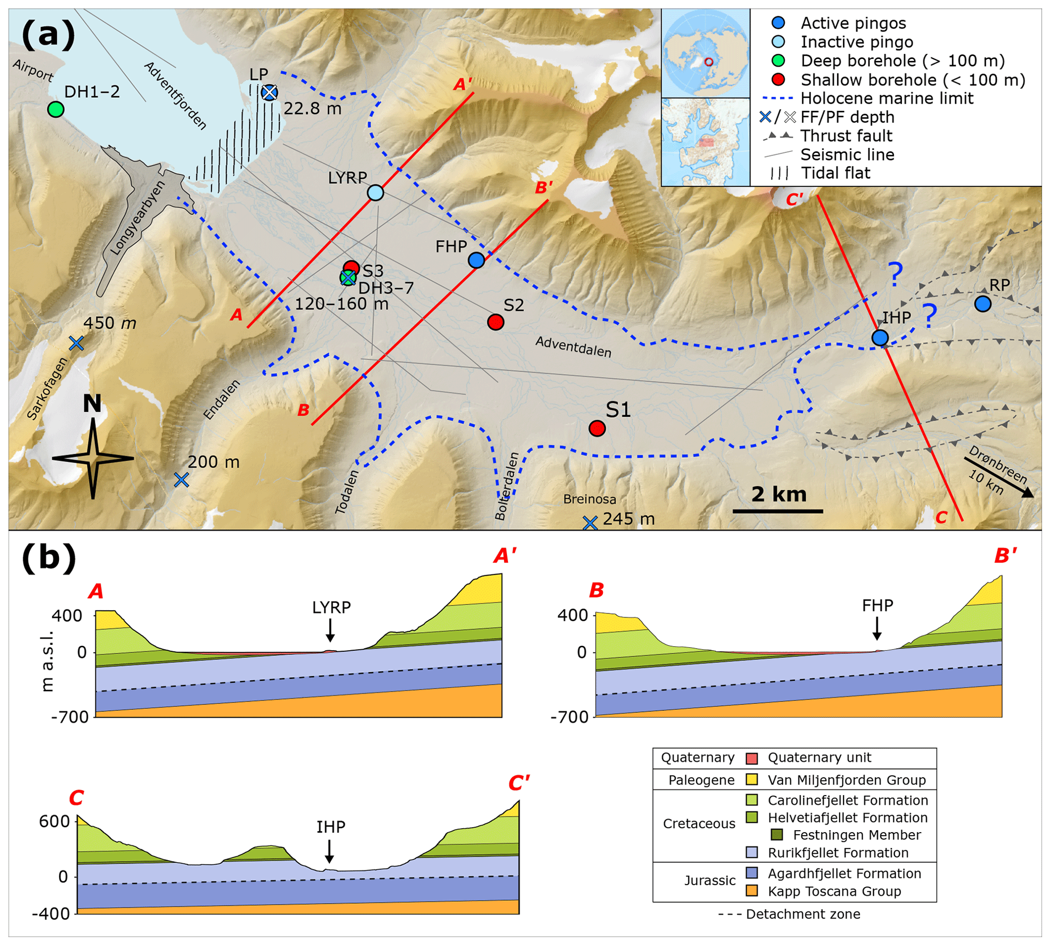
Figure 2(a) Map of lower Adventdalen with the location of data resources, pingos and the Holocene marine limit. LP: Lagoon Pingo; LYRP: Longyear Pingo; FHP: Førstehytte Pingo; IHP: Innerhytte Pingo; and RP: River Pingo. Core logs from boreholes S1–3 and D1–D7 (respectively, Gilbert et al., 2018, and Olaussen et al., 2020, and references therein), seismic lines (Bælum et al., 2012, and unpublished commercial lines from Norsk Hydro), and a geological map (Norwegian Polar Institute, 2019) were used to build the geological model (Fig. 5a) (see details in Hornum, 2018). Permafrost depth measurements at the Sarkofagen, DH4 and Breinosa sites are from Liestøl (1977), Braathen et al. (2012), and Christiansen et al. (2005), respectively. The freezing front depth at LP is from Yoshikawa and Harada (1995). Data used to develop the map including topography, glacial extent and fluvial network are courtesy of the Norwegian Polar Institute (2019). (b) Geological cross sections constructed based on the resources mentioned above. The Quaternary unit overlies well-consolidated sedimentary strata of pre-Cenozoic age (i.e. Cretaceous or older). See Sect. 3.1 for a (hydro)geological description of the layers shown in cross sections A, B and C.
Adventdalen is a ∼30 km long glacially cut valley in central Spitsbergen, Svalbard (Fig. 2a). Its high Arctic climate is characterised as polar tundra (Kottek et al., 2006), and the ground is dominated by continuous permafrost (Humlum et al., 2003). Because of the dry climate with a mean annual precipitation of ∼200 mm (Hanssen-Bauer et al., 2019), only a few, small glaciers exist today, the largest being Drønbreen, which is 9 km long and up to 200 m thick.
3.1 Geology and hydrogeology in Adventdalen
In Adventdalen, fine-grained Quaternary sediments (<70 m thick; Gilbert et al., 2018) overlie pre-Cenozoic, well-consolidated sedimentary strata (Fig. 2b), which are likely the best described in Svalbard largely thanks to the Longyearbyen CO2 Laboratory Project (Olaussen et al., 2020, and references therein). Together, all these units form a low-permeability groundwater system.
The sedimentary strata gently dip in a west-south-westerly direction (Fig. 2b), and the youngest strata are thus found closest to Longyearbyen and the present-day coastline. The uppermost unit, the Early Cretaceous Carolinefjellet Formation (Fm) (∼ 300 m thick; Fig. 2b), consists of sandstone intercalated with shale beds and overlies the fluvial sandstones of the Helvetiafjellet Fm (59–72 m thick; Grundvåg et al., 2019). The Festningen Member of the Helvetiafjellet Fm (11–18 m thick), comprises fractured sandstones and is relatively hydraulically conductive, as proven by cross-well water injection tests (Bælum et al., 2012). Directly below is the ∼450 m thick Janusfjellet Subgroup (Fig. 2b) that comprises two shale-dominated units, the Rurikfjellet (201–232 m thick; Grundvåg et al., 2019) and Agardhfjellet formations (253–264 m thick; Koevoets et al., 2018). A regional detachment zone with extensive fracturing and swelling clays propagates near the boundary of these two formations (Braathen et al., 2012) and is considered a major barrier to fluid migration (Olaussen et al., 2020). The tectonic disturbances, as reflected in Festningen Sandstone and the detachment zone, make it possible that a minor secondary permeability development is present elsewhere in the stratigraphy. This would have implications for groundwater movement in the system, which is otherwise predominantly through rocks with low hydraulic conductivity (Table 3).
The glacier advances during the last glacial maximum (LGM) on Svalbard (∼20 ka; ka =103 years before present) are thought to have completely eroded any pre-existing glacial deposits in the inner fjords of Svalbard (Elverhøi et al., 1995), and the Quaternary succession in Adventdalen thus postdates this event. Optically stimulated luminescence (OSL) datings in three cores from Adventdalen (S1, S2 and S3; Fig. 2a) support this (Gilbert et al., 2018). The Quaternary succession overlies fractures in the underlying sedimentary strata, possibly explained by glacier load/unload and freeze–thaw processes (Benn and Evans, 2010; Gilbert et al., 2018), as well as the significant tectonic uplift in the area. The presumed high hydraulic conductivity of this fracture zone is in contrast to the generally low permeability of the Quaternary succession. The lowermost Quaternary unit is a <5 m thick, subglacial lodgement till deposited during the last Weichselian glacial advance. Overlying the till, a shallowing-upward trend is observed in the gradually changing succession of marine muds (<20 m), pro-deltaic to deltaic muds and very fine-grained sands (< 35 m), tidally influenced (saline) fluvial fine-grained sands (<35 m), and aeolian loess deposits (<5 m). This reflects Holocene progradation of the present delta system (Cable et al., 2018; Gilbert et al., 2018).
The sub-permafrost groundwater often has hydraulic heads above hydrostatic heads, which results in artesian conditions. This is evident from the occurrence of several pingo springs and from artesian outflow from deep boreholes (> 100 m below ground level, b.g.l.) at the confluence of Bolterdalen and Adventdalen (Malte Jochmann, personal communication; SNSK, Unpublished Reports SN1981_008 and SN1983_004). Based on artesian outflow during a drilling experiment nearby, Braathen et al. (2012) deduce a hydraulic pressure of 18 to 23 bars at a depth of ∼175 m b.g.l. in well DH4 (Festningen Member; Fig. 2) which corresponds to a hydraulic head of 9 to 60 m above a hydrostatic head when the potential pressure effects of the dissolved gasses are excluded. Significant under-pressure Pa below hydrostatic is recognised in deeper stratigraphical layers (∼800 m b.g.l.) and is believed to relate to glacial unloading, extensive fracturing and matrix expansion (Birchall et al., 2020; Braathen et al., 2012; Wangen et al., 2016). The low pressure indicates hydrogeological separation from upper groundwaters immediately beneath the permafrost, which is in line with Sr isotope analyses from the drill cores (Huq et al., 2017; Ohm et al., 2019).
3.2 Late Weichselian and Holocene climate history
Air temperatures on Svalbard have been continuously recorded at Longyearbyen Airport since 1911 (Nordli et al., 2014). Until the 1990s, the 30-year running mean of MAATs was −6.0 ∘C, while it has increased to −4.2 ∘C in the period 1988 to 2017 (Hanssen-Bauer et al., 2019). For the entire temperature record, the mean summer air temperature (MSAT) has consistently been 10 ∘C warmer than the MAAT (on the 30-year scale; Førland et al., 1997). Further back in time, Holocene mean summer sea temperatures (MSST) in and around Svalbard are relatively well constrained by fossil-based temperature reconstructions (Fig. 3a; van der Bilt et al., 2018; Hald et al., 2007; Mangerud and Svendsen, 2017). Mangerud and Svendsen (2017) point out that the MSST is essentially identical to the MSAT.
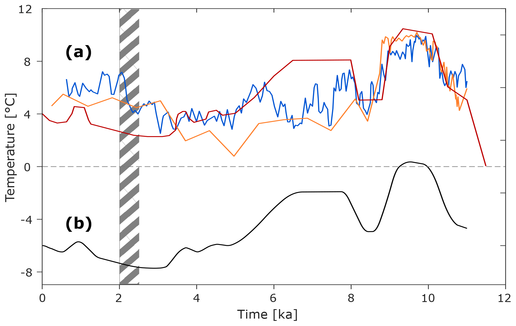
Figure 3Holocene temperature reconstructions in and around Svalbard. Dashed grey area indicates time of minimal driftwood arrival (Farnsworth et al., 2020). The unit of the time axis is ka =103 years before present. (a) MSST curves (= MSAT, see text): red line from Mangerud and Svendsen (2017), orange line from Hald et al. (2007), and blue line from van der Bilt et al. (2018). (b) MAAT used in this work, based on Mangerud and Svendsen (2017) and Førland et al. (1997) (see Sect. 4.3.3).
At the last glacial maximum (LGM) occurring at ∼20 ka, glaciers covered all fjords in Spitsbergen (Ingólfsson and Landvik, 2013). By ∼11.5 ka, the central parts of Isfjorden were glacier-free, and its inner tributaries followed at ∼11.2 ka (Forwick and Vorren, 2011; Gilbert et al., 2018). If any glacier ice remained in Adventdalen after then, it was certainly gone by ∼10 ka when non-glacial sediments were deposited in the valley head (Lønne and Nemec, 2004). The eustatic sea level rise caused by Northern Hemispheric deglaciation during the late Quaternary and Early Holocene was surpassed on Svalbard by the rate of its postglacial rebound. The Holocene marine limit (HML) ranges from ∼20 m above sea level (a.s.l.) in the north-western part of Spitsbergen to ∼90 m a.s.l. in the central part (Forman, 1990). In Adventdalen, raised marine sediments suggest a HML of ∼62 m a.s.l. and ∼70 m a.s.l. in the inner and outer parts of the valley, respectively (Lønne and Nemec, 2004). Although not well constrained, the relative sea level is estimated to have fallen pseudo-exponentially until reaching close to present levels by ∼5 ka (Lønne and Nemec, 2004). Despite the uncertainty of sea level fall, the fjord retreat and the associated exposure of the new valley floor are relatively well constrained by absolute dating presented in previous work (Table 1).
Table 1Absolute ages from Adventdalen constraining delta propagation.
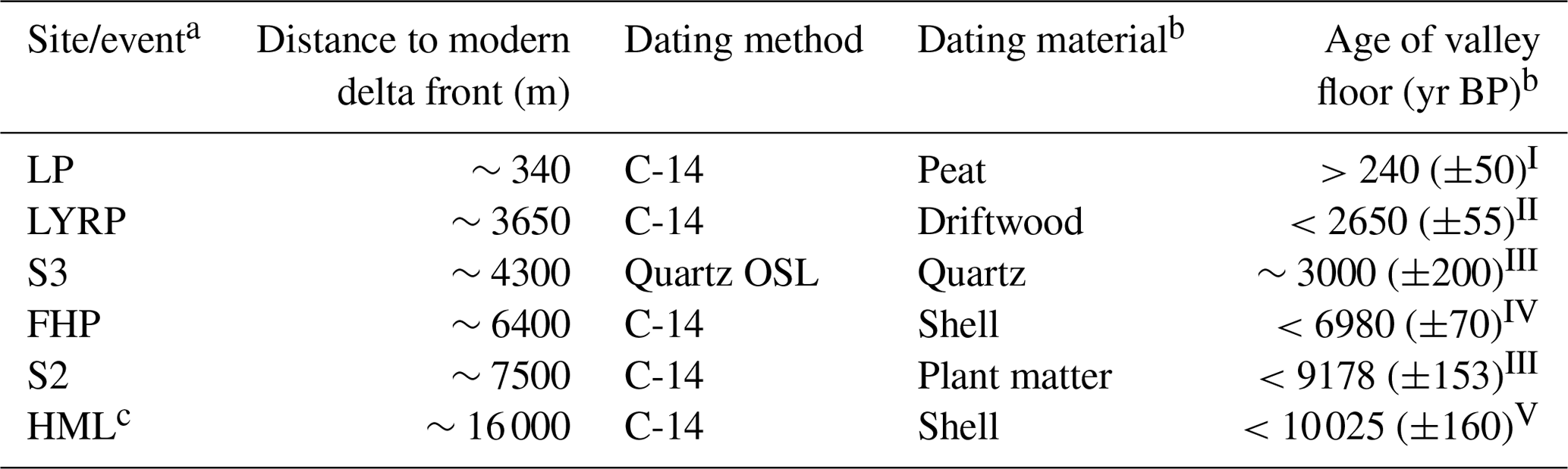
a See Fig. 2 for site locations. b Depending on the dated material and the host sediment, the dating indicates minimum, approximate or maximum valley floor ages. c HML: Holocene marine limit. Compiled from I Åhman (1973), II Svensson (1970), III Gilbert et al. (2018), IV Yoshikawa and Nakamura (1996), and V Lønne and Nemec (2004).
3.3 Permafrost, pingos and the apparent lack of groundwater recharge
In the valley floor of Adventdalen, the permafrost thickness ranges from ∼0 m at the coast to ∼200 m inland. In the adjacent mountains, it increases to >450 m (Christiansen et al., 2005; Humlum et al., 2003; Liestøl, 1977). One observation of the freezing front depth at Lagoon Pingo (Harada and Yoshikawa, 1996) and permafrost depth observations at well DH4 (Braathen et al., 2012), Endalen, Sarkofagen (both Liestøl, 1977) and Breinosa (Christiansen et al., 2005) support this regional characterisation (Fig. 2a). Mountain permafrost is presumably of Weichselian age, while permafrost in valleys postdates the Late Holocene (Humlum, 2005). The continuous permafrost and a lack of warm-based glaciers in the adjacent highlands most likely hinder subglacial recharge to the sub-permafrost aquifer due to the impervious frozen ground (Burt and Williams, 1976; Haldorsen et al., 2010; McCauley et al., 2002; Walvoord and Kurylyk, 2016; Woo, 2012).
Sub-zero temperatures are a prerequisite for permafrost formation, and its thickness essentially reflects equilibration to the geothermal heat flow (French, 2017). In the Adventdalen area, measurements of the geothermal gradient range from 0.02 ∘C m−1 in the highlands to 0.03 ∘C m−1 in the valley bottoms (Betlem et al., 2019; Liestøl, 1977).
Open-system pingos are a common feature in Svalbard and Adventdalen (Humlum et al., 2003), where five of them are distributed parallel to the valley axis (Fig. 2a). The three outermost – Lagoon, Longyear and Førstehytte pingos – are all located on the north-eastern side of the valley. All three have formed in Quaternary marine muds (Yoshikawa and Harada, 1995) and close to the sedimentary bedrock boundary (Fig. 2b). In the valley head, two additional pingos are located close to the boundary of HML: Innerhytte and River pingos. They have formed in shales above a major fault and are situated in the valley floor in the path of the river Adventelva (Yoshikawa and Harada, 1995). With the exception of the seemingly inactive Longyear Pingo, groundwater has discharged perennially from springs located at the pingos, at least since the earliest recordings in the 1920s (Orvin, 1944). However, visible spring outflow (or winter icing) at Førstehytte Pingo was not observed from summer 2018 until October 2019. Presumably, during that time, groundwater flow through the permafrost continued, but instead of discharging to the surface, groundwater froze within the pingo and added to its growth. From Lagoon Pingo, Yoshikawa and Harada (1995) reported a spring discharge of 0.013 to 0.016 L s−1, Hodson et al. (2019) estimated ca. 0.3 L s−1 during the 2017 summer, and we measured 0.26 L s−1 in August 2019. At Innerhytte Pingo, Yoshikawa and Harada (1995) measured a discharge rate of 0.11 L s−1, which is somewhat smaller than the estimate of Liestøl (1977) in 1976 of ∼1 L s−1. Based on our own “by eye” estimates involving no quantitative measurements, the discharge rate at Førstehytte Pingo was in orders of 0.1 L s−1 when visited in the fall of 2015, 2016 and 2017 and less than 0.01 L s−1 when rediscovered in October 2019.
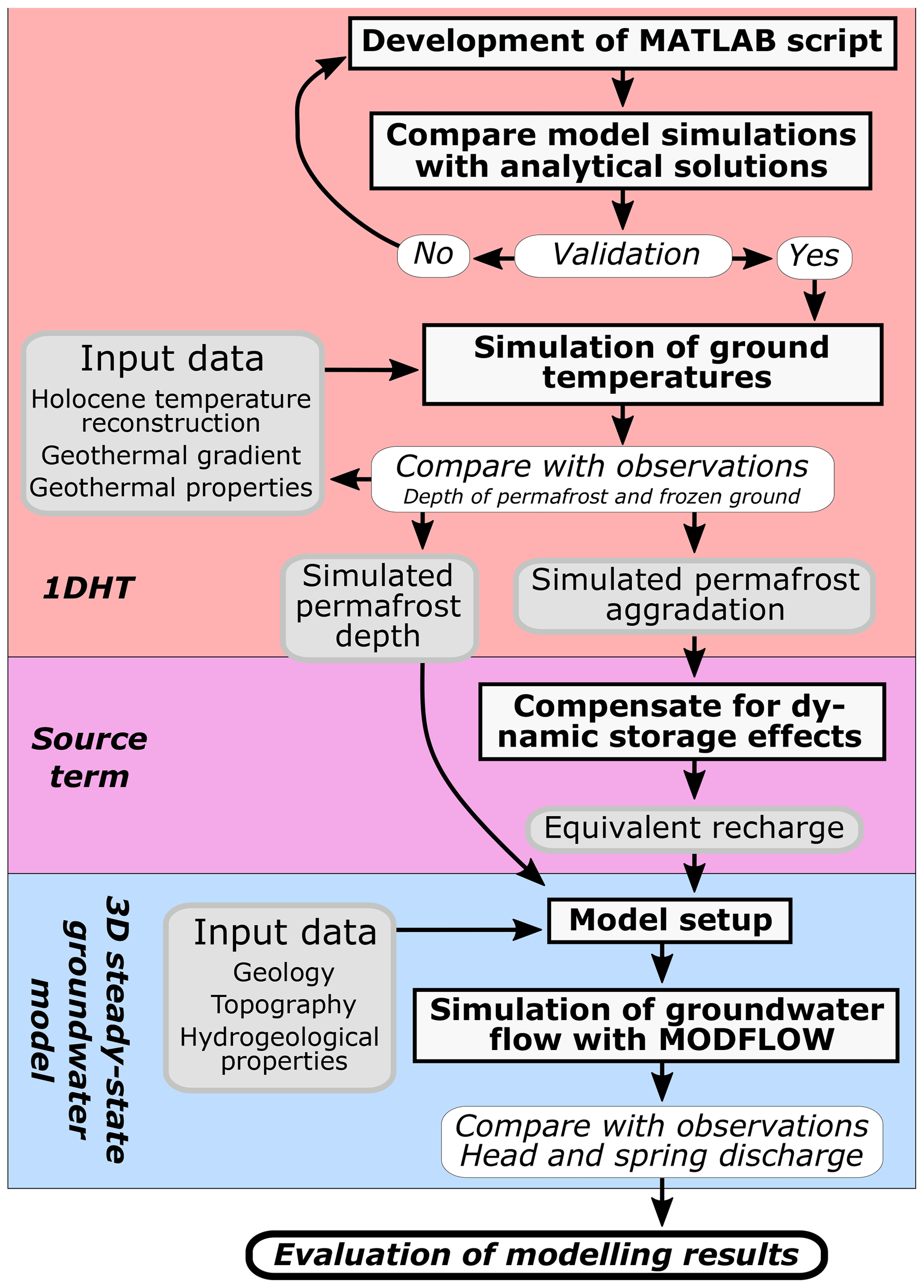
Figure 4Schematic overview of the inner workings of the decoupled heat and groundwater model. Model setup, calculations and algorithms are indicated with sharp corners and bold text. Validation and comparison of simulations and observations are indicated with round corners and italics. Input and output data are indicated with rounded corners, grey background and normal text.
Several numerical model codes are capable of simulating coupled heat and groundwater transport in permafrost environments (Grenier et al., 2018). However, the benchmark models do not consider the overpressure produced by ice expansion. To include this process, we decoupled the modelling of heat flow from sub-permafrost groundwater flow and made use of a source term to mimic the pressure effects of permafrost aggradation (Fig. 4). Ground temperatures and permafrost dynamics were simulated in the vertical dimension using a custom made finite-difference one-dimensional transient heat transfer model (hereafter just 1DHT) coded in MATLAB R2019b (MathWorks®, 2019). The 1DHT model script is publicly available at https://doi.org/10.5281/zenodo.4240594. Groundwater flow was modelled in a three-dimensional steady state with MODFLOW in the groundwater modelling software GMS 10.4 (AQUAVEO™, 2019). The connection between the two models was the permafrost aggradation rates simulated by the 1DHT which determined the only water source for the groundwater model. The decoupled approach does not simulate advective or lateral heat transport. The potential limitations will be assessed in the Discussion (Sect. 6.2.1).
4.1 Heat flow
Heat flow was modelled one-dimensionally in the vertical dimension, which is a common approach for permafrost models (Riseborough et al., 2008). Following from Fourier's law and conservation of energy, the one-dimensional conductive heat flow equation states that
where T is temperature (K), t is time (s), z is distance (m), and ke, ρe and ce are the effective values of the thermal conductivity (W (m K)−1), density (kg m−3) and specific heat capacity (J (kg K)−1), respectively. The term equates to αe, the effective thermal diffusivity (m2 s−1). As heat transfer was modelled one-dimensionally, simulating advective heat transfer was not possible. The ratio of advection to conduction heat transfer rates may be quantified by a Péclet number (Bergman et al., 2011):
where v is the pore water velocity and L is the characteristic length.
In the case of a saturated medium, heat will be conducted through a matrix of solids (i.e. sediment or rock) and liquid water, ice or a mixture. The effective thermal parameters were assumed independent of temperature, but the fractions of water and ice changed between the solidus and liquidus temperatures, TS and TL, respectively. The fraction of liquid water within the pore space, fw, was determined using a smoothed step function (same approach as Mottaghy and Rath, 2006):
where w (K) determines the shape of the freezing curve. For this work, w≈0.96, implying that ∘C and TL=0 ∘C. Bonacina and Comini (1973) and Mottaghy and Rath (2006) note that the exact shape of the freezing curve is of little importance for the calculated temperatures but that a smoother function generally improves the performance of a numerical model due to a more efficient convergence of the numerical approximation. The total fractions of soil or rock (Fs), water (Fw), and ice (Fice) are described respectively as , , and , with n being the total porosity. The effective thermal conductivity was calculated as the root square mean, as done by Mottaghy and Rath (2006) and Govaerts et al. (2016). When temperature change occurs between TS and TL, freezing or thawing results in the release or absorption of latent heat (L=333.6 kJ kg−1; Mottaghy and Rath, 2006). The latent heat of fusion was included in the expression of the equivalent volumetric heat capacity (Ceq in J (m3 K−1); same approach as Govaerts et al., 2016):
where subscripts “s”, “w” and “ice” indicate parameters of soil or rock, water, and ice, respectively.
To validate the model code, we compared simulations with two analytical solutions: Neumann's solution as presented by Carslaw and Jaeger (1959) and Mottaghy and Rath (2006) and an analytical solution of a step change in temperature neglecting latent heat effects as presented by Carslaw and Jaeger (1959) and Eppelbaum et al. (2014). The model code was able to reproduce the analytical results with root mean square errors of, respectively, and , and these numbers were regarded as representing an acceptable level of accuracy for the given purpose. The model code validation is described in detail in the Supplement.
4.2 Groundwater flow
Following from Darcy's law and the conservation of mass, the three-dimensional groundwater flow equation fundamental for groundwater modelling can be described as follows (Fitts, 2002):
where x, y and z are distances (m) in the three dimensions, the K values are hydraulic conductivities (m s−1) in those dimensions, h is the hydraulic head (m), QN is a term representing any potential sink or source (m3 s−1; i.e. recharge, seepage, etc.), Ss is the specific storage, and t is time (s). In this work, groundwater flow was modelled as a steady state implying that the right-hand side of Eq. (5) equals 0. However, in the discussion of the model simulation results, hydrodynamic storage effects resulting from the glacial loading and unloading are considered.
Groundwater flow was simulated with MODFLOW, which solves the three-dimensional groundwater flow equation with the finite difference method (McDonald and Harbaugh, 1988). We approximated the pressure build-up from the simulated rate of permafrost aggradation (RPF) by considering that it must correspond to some equivalent recharge rate (REq) or source term (QN in Eq. 5). Assuming no expansion or compression of the matrix, REq is specifically proportional to RPF, the total porosity (n) and the expansion of water upon freezing (Xw):
where is equivalent to the source term QN in Eq. (5), and A is an area (m2).
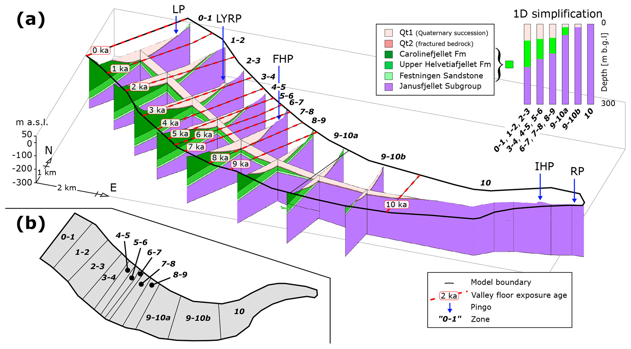
Figure 5(a) Three-dimensional geological model of the subsurface below the valley floor in Adventdalen and vertical one-dimensional simplifications (inset in upper right corner) below zones of the model area. The former determines the hydrogeological properties in the groundwater model (Table 3), whereas the latter determines the geothermal properties in the 1DHT model (Table 2). The domain of the 1DHT model extends to 1000 m b.g.l. (not shown). Deeper than 300 m b.g.l., geothermal properties were defined like those for the Janusfjellet Subgroup. The sea retreat reconstruction was inferred from absolute datings (Table 1) and is illustrated by valley floor exposure isochrones (dashed red lines). Pingos are indicated with blue arrows. (b) Vertical view of the model area showing the zonation. The aforementioned isochrones defined the zone names so that the valley floor exposure age of a zone is apparent from its name (i.e. zone 0–1 became sub-aerially exposed between 1 and 0 ka, zone 1–2 between 2 and 1 ka, etc.).
4.3 Setup and boundary conditions
4.3.1 Geological model
In order to define proper geothermal and hydrogeological properties, a geological model of the subsurface in Adventdalen was built. Towards the north-west, the model covers the tidal flat (Fig. 2a), but no other sea-covered areas were included. Elsewhere, the horizontal model boundary was a simplified outline of the HML. The lower boundary is at 300 m b.g.l. (Fig. 5a). We used data from boreholes, seismic lines (see locations and references in Fig. 2a) and a geological map with a digital elevation model (DEM) provided by the Norwegian Polar Institute (2019). The general workflow was to map relevant geological boundaries in three-dimensions with the petroleum industry software Petrel v2016 (Schlumberger©, 2019) then use them to build geological layers with the TIN and SOLIDS editor functions of GMS 10.4 (AQUAVEO™, 2019). For the 1DHT model, the geology was simplified into one-dimensional columns for a total of 12 zones of the model area. The zones were defined as follows. The age of the valley floor (Table 1) was used to infer isochrones of valley floor exposure at intervals of 1000 years (Fig. 5a). The isochrones defined boundaries between the zones and the names of the zones (i.e. the zone located between the 5 and 6 ka isochrones was named zone 5–6; Fig. 5b). The area between isochrones 9 and 10 ka was divided into two zones (9–10a and 9–10b) to incorporate geological variation.
Table 2Geothermal material properties used in the heat transfer model.
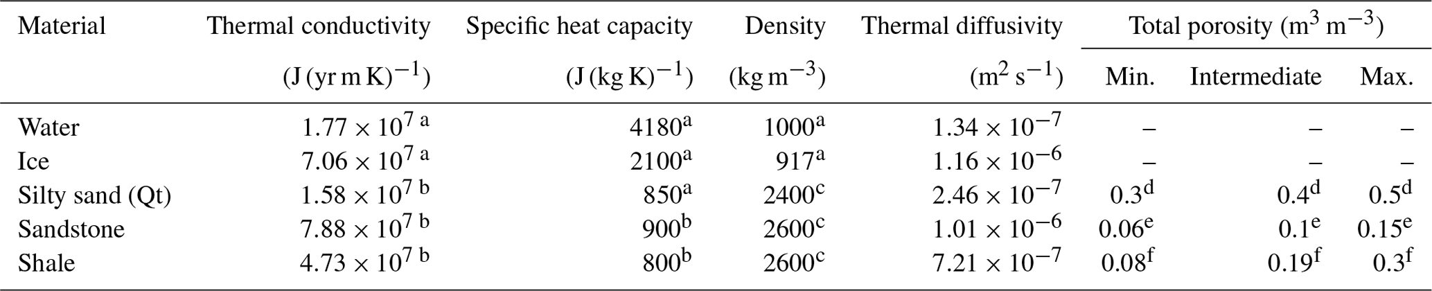
Density and thermal properties compiled from a Williams and Smith (1989), b Robertson (1988), and c Manger (1963). Porosities from d Fitts (2002) and e Braathen et al. (2012) and based on works by f Burland (1990), Grundvåg et al. (2019), Marshall et al. (2015), Okiongbo (2011), and Yang and Aplin (2004) (see text for more detail).
Table 3Properties of the hydrogeological units used in the groundwater model.
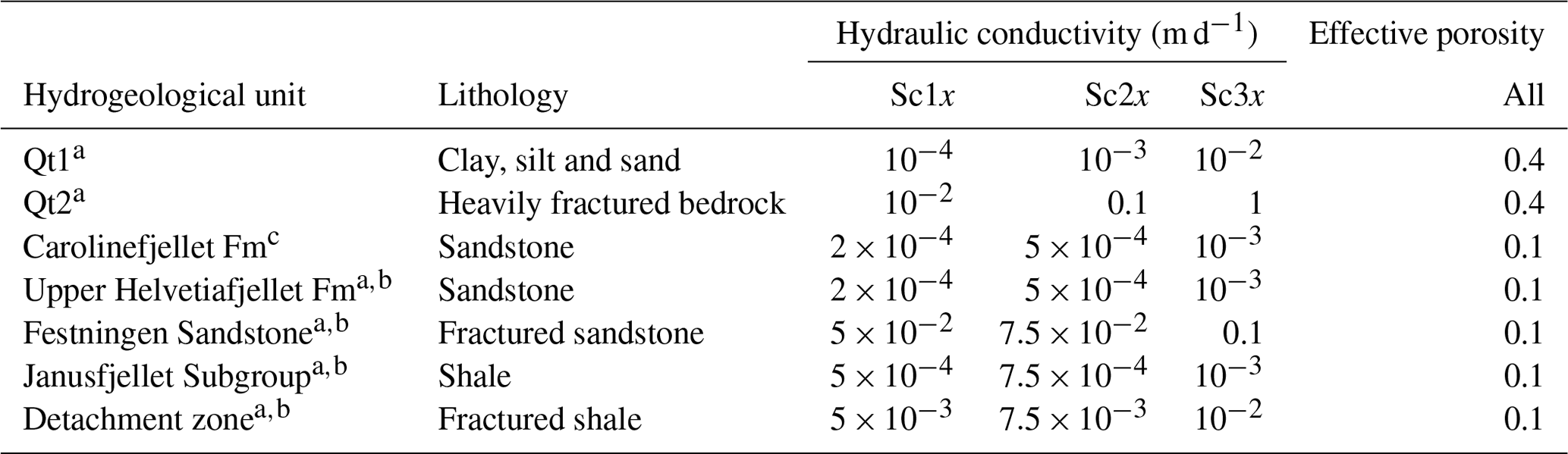
Property values based on a Fitts (2002) and b Singhal and Gupta (2010) or evaluated from c Braathen et al. (2012) (details provided in the Supplement).
4.3.2 Geothermal and hydrogeological properties
Due to the sparse data available from the field area, geothermal and hydrogeological properties of the lithologies in the model domain (Tables 2 and 3) were largely based on the available literature. The considerable contrast between the thermal properties of water and ice implied that porosity was the most important parameter for permafrost growth, and realistic minimum, intermediate and maximum values were therefore defined for the 1DHT model (Table 2). The permafrost base is presently located within the upper two-thirds of the Janusfjellet Subgroup (Figs. 2b and 5a). Estimated burial depths and thicknesses of overlying units (Grundvåg et al., 2019; Marshall et al., 2015) indicate that this stratum has been buried to maximum depths between 2150 and 2600 m b.g.l. corresponding to effective vertical stresses between 34 to 41 MPa (assuming a rock density of 2.6 kg m−3 and hydrostatic equilibrium). Different studies on the compressibility of lithologically and age-equivalent rocks in the North Sea thus suggest porosities between 0.08 to 0.3 (Burland, 1990; Okiongbo, 2011; Skempton, 1969; Yang and Aplin, 2004). We therefore used this range in our modelling experiments. An exception to the purely literature-based values is the sandstone units whose matrix porosity and vertical permeability, κv, were measured as part of the Longyearbyen CO2 Laboratory Project (Olaussen et al., 2020, and references therein). The small-scale horizontal permeability, κh, for sandstone is typically a factor of 2 higher than κv (Domenico and Schwartz, 1998). The horizontal hydraulic conductivity, Kh, was therefore calculated using the measurements of κv by Braathen et al. (2012) as
where is the conversion factor (i.e. 2 for this work), κv is permeability (m2), ρw is the density of water (kg m−3), g is the gravitational acceleration (m s−2), and μ is the dynamic viscosity of water (kg (m s)−1). The range of the hydraulic conductivity values of the Carolinefjellet and Helvetiafjellet formations (Festningen Sandstone not included) was defined by the 25 %, 50 % and 75 % percentiles of a log-logistic probability fit of the measured values (details provided in the Supplement). Ranges of hydraulic conductivity for the fluvio-deltaic succession were based on literature values from Fitts (2002). For the remaining bedrock units, we also regarded the influence of fractures (Singhal and Gupta, 2010). All within these ranges, three sets of hydraulic conductivity defined the different model scenarios (Sc1–3x; Table 3). For steady-state simulations, the porosity does not affect the net groundwater fluxes (i.e. discharge and Darcy fluxes; Eq. 5). To evaluate the pore water velocities, however, the effective porosity is of importance. We used the same values of effective porosity for all groundwater model simulations (Table 3).
4.3.3 One-dimensional transient heat transfer model (1DHT)
The model domain contained 12 columns, each 1000 m long and consisting of 500 cells with a height of 2 m. One column was associated to each of the model area zones, and the geothermal properties were defined according to the associated geological one-dimensional simplifications (see insert in Fig. 5a). Deeper than 300 m b.g.l., the properties were like those of the Janusfjellet Subgroup. The simulation runtime was defined by the valley floor age inferred for that zone (Fig. 5) so that for zone 0–1 the simulation period was 0.5 to 0 ka, for zone 1–2 it was 1.5 to 0 ka, etc. For zone 10, the simulation period was 10 to 0 ka. The initial ground temperature distribution followed the geothermal gradient reported by Liestøl (1977) (0.025 ∘C m−1) from a surface temperature of 0 ∘C. At any subsequent time, the lower boundary condition was defined from the same geothermal gradient, resulting in a basal temperature change of less than 0.65 ∘C. The upper boundary condition was defined by the Holocene MAAT curve presented in Fig. 3b. Assuming that the present 10 ∘C difference between MAAT and MSAT (Førland et al., 1997) was alike for the entire Holocene, we constructed this curve (Fig. 3b) by subtracting 10 ∘C from the MSST curve by Mangerud and Svendsen (2017) (Fig. 3a). As illustrated in Fig. 3a, their MSST curve is largely in agreement with MSST temperature reconstructions from the west and south-west of Svalbard (van der Bilt et al., 2018; Hald et al., 2007). We chose to rely on Mangerud and Svendsen (2017) because (a) their curve is more local to our field area than the alternatives and (b) the suggested timing of the Holocene thermal minimum at ∼3 to 2 ka is in agreement with the maximum of perennial or semi-permanent landfast sea ice at ∼2.5 to 2 ka inferred from the minimal occurrence of dated driftwood (Dyke et al., 1997; Farnsworth et al., 2020; Funder et al., 2011). Furthermore, their curve is better supported by geomorphological evidence of glacier dynamics (Farnsworth et al., 2020).
4.3.4 Groundwater model
For the groundwater model, each grid cell measured 100 by 100 by 5 m (xyz), and their hydrogeological properties were defined from the geology (Fig. 5a, Table 3). The model domain was defined from the geological model, therefore covering an elongated ground surface area of 59 km2 that is <4 km broad and ∼18 km long (Fig. 5b). Frozen ground was considered impervious, and cells shallower than the simulated freezing front depth were thus de-activated. The lower boundary was at 300 m b.g.l. The fjord was simulated with a general head of 0 m a.s.l. and the conductance was determined according to the hydraulic conductivity (Table 3). The area assigned with these boundary conditions comprised 24 cells located within the uppermost layer at the north-western end of the model domain. The MODFLOW drain package was used to simulate pingo springs. Because the cells located at the springs were inactivated, the drains were assigned to the uppermost active cells located closest to springs but within the conductive Festningen Sandstone if present in the underlying stratigraphy (i.e. Lagoon and Førstehytte pingos; Fig. 5a). Drain levels were set according to spring elevations (i.e. 1, 20, 65 and 77 m a.s.l. for Lagoon, Førstehytte, Innerhytte and River pingos, respectively). The simulated springs were able drain more water than the cells they were situated in could transmit. That is, the conductance was set high enough not to restrict any discharge. Except for the fjord and the springs, all outer model boundaries were assigned no-flow conditions.
The only source of water in the groundwater model was defined from the basal permafrost aggradation rate simulated by the 1DHT model and assigned as recharge to the uppermost active cells in the model domain. To compensate for the lack of dynamic storage effects in the steady-state model, we applied a moving time average to the simulated basal permafrost growth (or decay) before calculating the recharge equivalent (Eq. 6). The time window of the moving average was based on the possible range of the adjustment time, ta, which is the time needed for fluids to redistribute to a pressure perturbation (e.g. Neuzil, 2012; Šuklje, 1969):
where l is half of the shortest dimension of the system (the characteristic length), Ss is the specific storage, and K is the hydraulic conductivity. We found ta to be shortest in the vertical dimension but assumed that hydraulic pressures could only dissipate in the horizontal dimension after the formation of continuous permafrost no earlier than 6 ka (Humlum, 2005; this research). Specifically, we estimated the horizontal ta to be between 20 and 19 000 years. To quantify this, we used a characteristic length of 1 km. For Ss, we used a matrix compressibility of to Pa−1 (based on common estimates for fractured rocks; e.g. Domenico and Mifflin, 1965; Domenico and Schwartz, 1998; Fitts, 2002) yielding a Ss of to m−1 (in line with literature values; cf. Singhal and Gupta, 2010). For K, we used the values estimated for the dominating geological unit (Janusfjellet Subgroup; Table 3). The time window used to compensate for dynamic storage effects were defined from the above but no longer than the age of permafrost (i.e. 6000 years or less).
To represent the uncertainty of how permafrost aggradation affects sub-permafrost groundwater flow, we simulated nine different scenarios that were defined by having three sets of values for the two fundamental parameters in any combination: hydraulic conductivity (scenarios Sc1–3x; Table 3) and equivalent recharge (scenarios ScXa–b; values calculated as described above and by Eq. 6). The nine scenarios are all labelled ScXx where X and x indicate the minimum, intermediate or maximum value sets of hydraulic conductivity and equivalent recharge, respectively. We further simulated a tenth scenario that takes additional pressure sources into account.
5.1 1DHT model results
The direct output from running the 1DHT model code was matrices containing the temperatures throughout the model domain for each time step in the simulation period. For each time step, the permafrost and freezing front depths were calculated by interpolating the depth at which the associated temperatures occurred. The greatest phase change rate in the 1DHT model occurs at a temperature of −0.7 ∘C (following from Eq. 3), and it was therefore the progression rate of this isotherm that was used for the calculation of the equivalent recharge (by net pore space loss; Eq. 6). Hereafter, “permafrost aggradation” therefore means the downward progression rate of this isotherm (−0.7 ∘C), although this is not entirely congruent with the thermal definition of permafrost (ground perennially below 0 ∘C; French, 2017). Since phase change occurs over a temperature range, the porosity used to calculate the equivalent recharge was taken as a weighted mean of the porosities in the corresponding cell range, in which the weight was proportional to the phase change rate.
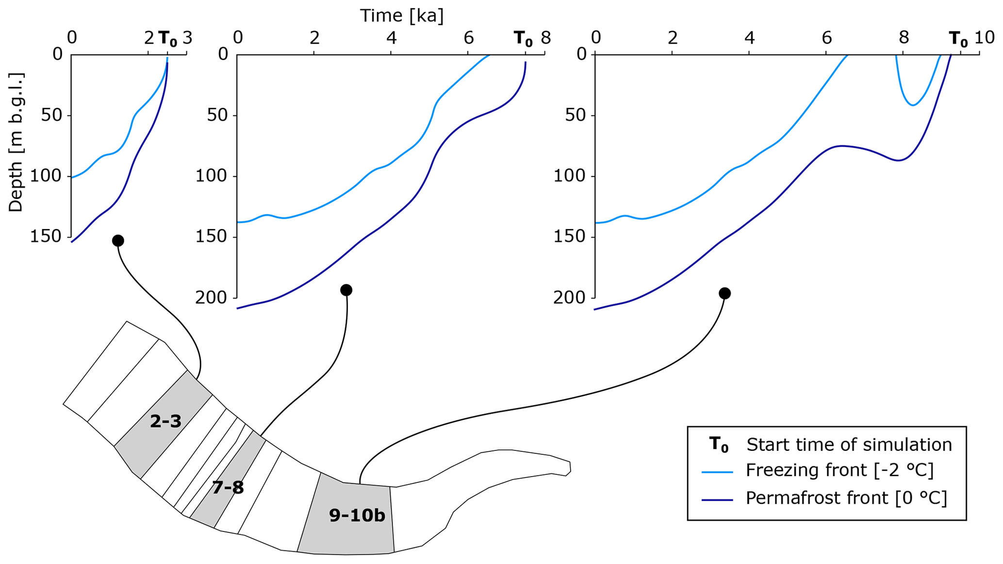
Figure 6Development of simulated freezing front and permafrost front depths from zones 2–3, 7–8 and 9–10b of the model area (see Fig. 5). These simulation results are derived when using the intermediate porosity values (Table 2). Note that completely frozen ground does not establish permanently until ∼6.5 ka.
5.1.1 Permafrost and freezing front depth
In Fig. 6, the simulated Holocene ground temperature development in Adventdalen is exemplified by the growth of frozen ground and permafrost in zones 2–3, 7–8 and 9–10b when using the intermediate porosity values (Table 2). For the oldest part of the model area (most inland), an early occurrence of frozen ground was simulated during the Early Holocene cooling of 9 to 8 ka (Figs. 3 and 5). However, due to the subsequent warming from 8 to 6.5 ka, frozen ground was thawed and not re-established until ∼6.5 ka. From this time, deep ground temperatures were simulated to be cooling until the present. The pattern was identical for simulations with lower and higher porosities (not shown), although the depths were different (as illustrated in Fig. 7a).
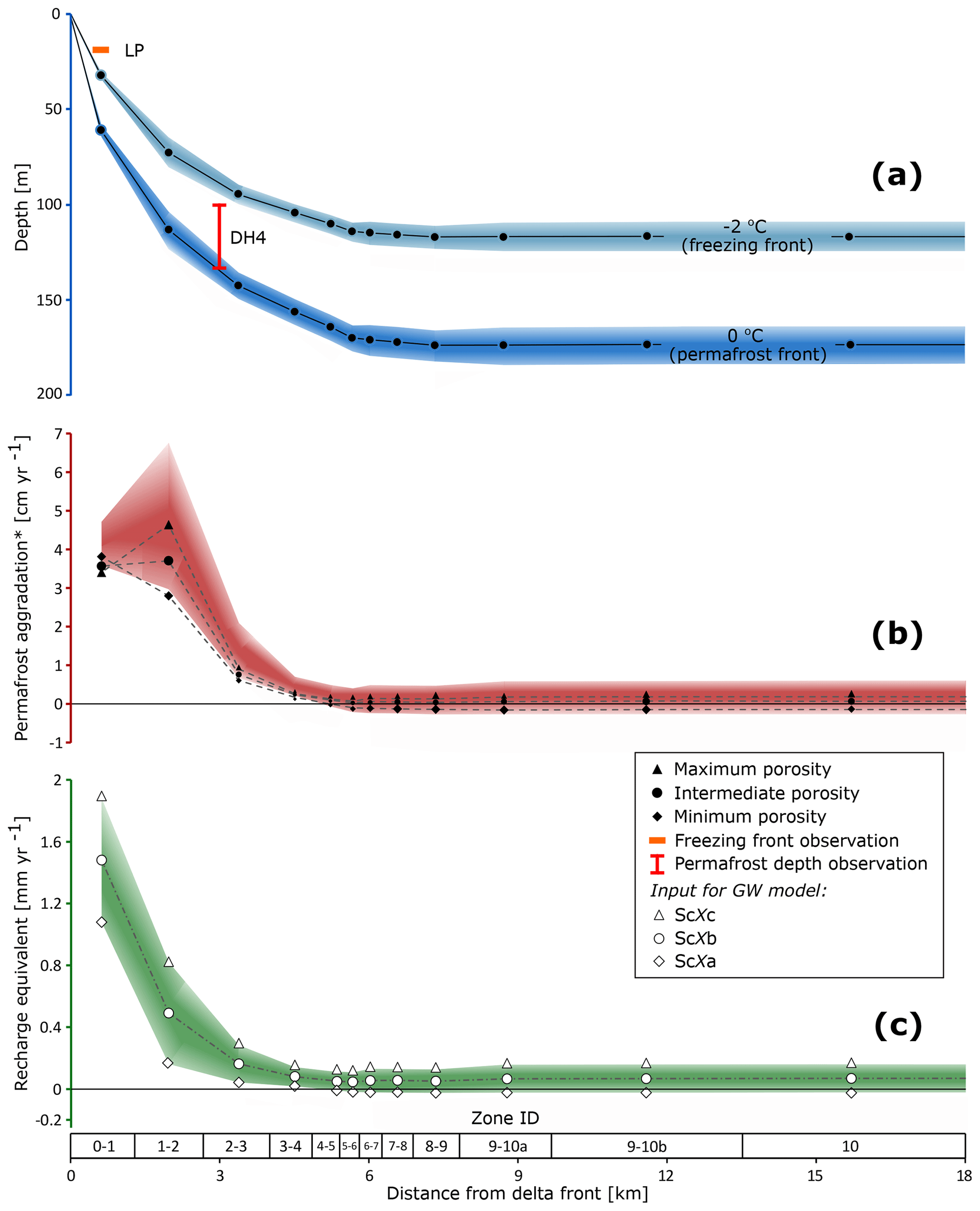
Figure 7Present-day permafrost conditions as simulated by the 1DHT model. (a) Freezing front and permafrost depths. The upper and lower edges of the shaded area correspond to the maximum and minimum limits of the porosity range, while the curve and the points correspond to the intermediate limits (Table 2). Permafrost depth and freezing front depth observations are from Braathen et al. (2012) and Harada and Yoshikawa (1996), respectively. (b) Rate of permafrost aggradation. The point symbols represent the present permafrost aggradation, while the shaded area is drawn by applying a time-moving average, as described in Sect. 4.3.4, and represents the values used to calculate the equivalent recharge rates. * The −0.7 ∘C isotherm, which has been used to calculate this, since the greatest phase change rate takes place at that temperature. (c) Equivalent recharge rate (net rate of loss in pore space). The points on the curve and the outer edges of the shaded area represent the recharge rates, which were assigned to the corresponding zones in the groundwater model.
Depending on the scenario, the 1DHT model simulated present day permafrost and freezing front depths of, respectively, 165 to 184 and 110 to 124 m b.g.l. at distances further than 6 km from the delta front (Fig. 7). Closer to the delta front, both isotherms are located at shallower depths and decrease from 58 to 65 and 31 to 34 m b.g.l. The porosity plays an important role for the temperature development due to latent heat of the water (ice) filling the pore space and because water and ice account for the minimum and maximum thermal diffusivities in the model domain, respectively. In panel (a) of Fig. 7, an uncertainty field is drawn (shading), as derived from the applied porosity range (Table 2). The upper and lower edge of the shaded area corresponds to the maximum and minimum porosity. The line corresponds to the intermediate porosity (Table 2). In panel (b), the simulated present permafrost aggradation rate is plotted by point symbols. The shaded area was drawn by applying the moving time-average correction defined using the estimated adjustment times (see Sect. 4.3.4, Eq. 8), and it indicates the values used to calculate the equivalent recharge rates in panel (c). Here, the line indicates intermediate values of recharge added to the groundwater model, while the edges of the shaded area represent the lower and upper estimates. The scarcity of ground temperature observations does not allow for model calibration, but observations both at Lagoon Pingo (freezing front) and well DH4 (permafrost) agree relatively well with the simulations.
5.1.2 Permafrost aggradation and recharge equivalent
Simulated rates of present permafrost aggradation ranged from −0.02 to 5 cm yr−1 and generally decreased up-valley with older exposure ages and for scenarios with lower porosity (Fig. 7b). The correction for dynamic storage effects generally increased the “effective” permafrost aggradation rate that was used to calculate the recharge equivalent. The reason for this was that basal permafrost growth was generally faster in the past (Fig. 6). For a homogeneous medium with one-sided freezing, the freezing front progression rate will decrease with time (as exemplified by Fig. S2). At first, it therefore seems surprising that the model simulations generally did not suggest that the highest aggradation rate occurred where permafrost is youngest (zone 0–1) but instead at zone 1–2. This was due to the heterogeneity in the model domain as expressed by the different properties of the sediments and bedrock undergoing freezing. In zone 0–1 closest to the shore, phase change took place at <60 m b.g.l. corresponding to the most porous and least thermally diffusive unit (Qt1; insert in Fig. 5a and Table 2). Thus, a relatively high amount of latent heat had to be released for the freezing front to aggrade. By contrast, the opposite was the case in zone 1–2, where the freezing front just entered the sandstone unit that possessed the lowest porosity (Carolinefjellet Fm; insert in Fig. 5a and Table 2). For the same reason, Fig. 7c shows that the pattern of the equivalent recharge decreases from 1.1 to 1.9 mm yr−1 closest to the delta front (zone 0–1) to −0.02 to 0.16 mm yr−1 in zone 10 furthest up-valley.
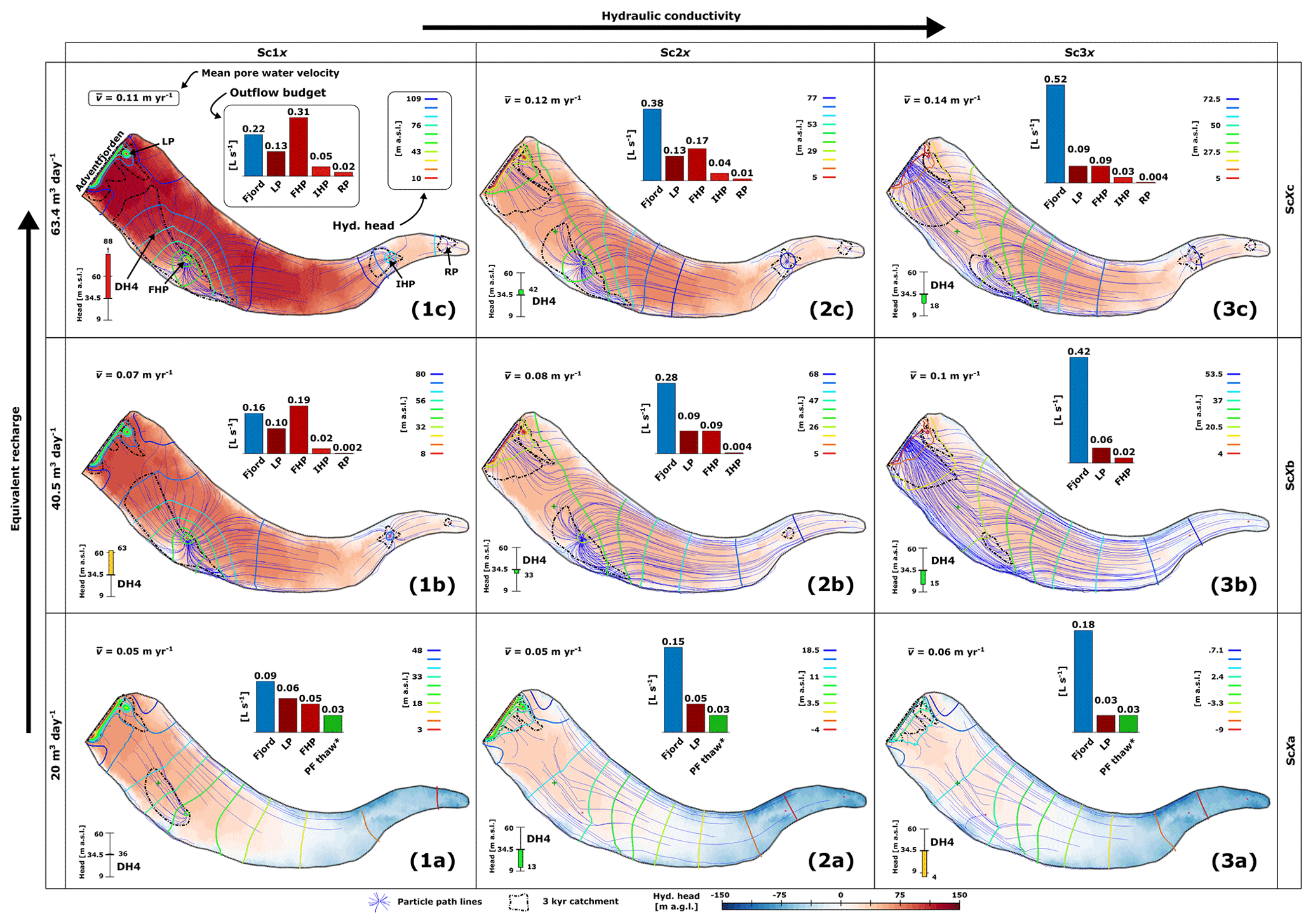
Figure 8Groundwater model simulations from all nine scenarios. The individual diagrams are sorted so that the hydraulic conductivity increases along the right-hand axis (scenarios Sc1–3x) and the equivalent recharge produced by permafrost aggradation increases along the left-hand axis (scenarios ScXa–c). On each diagram, the following simulation results are illustrated: heads from the uppermost grid layer are shown in metres above sea level (m a.s.l.) by isopotential contours (note that the colour scales are different) and in metres above ground level (m a.g.l.) by the colour fill (see scale at the bottom of the figure). The latter indicates if artesian conditions are simulated (reddish) or not (blueish). The groundwater outflow rates and distribution are illustrated by bar charts with the location of the discharge points (pingos and fjord) indicated in (1c). For minimum scenarios (1a, 2a, 3a), part of the outflow represents phase change associated with permafrost thaw (Fig. 7b–c), which causes a storage redistribution within the model domain. Flow patterns are illustrated by thin blue lines which each depict pathways of particles released in the uppermost grid layer. The mean pore water velocities, shown in the upper left-hand corners, were calculated from the aforementioned particles and using the same porosities for all scenarios (Table 3). The thick dashed lines outline the areas (catchments) that contributed water to the outlet points during 3 kyr of simulation time. In the lower right-hand corner, the simulated head in well DH4 is illustrated on a range plot with the range defined like that deduced from Braathen et al. (2012). The colour of the bar indicates if the simulated head falls within (green) or outside the deduced range with less (yellow) or more (red) than 10 % of the total range. The location of DH4 and the pingo springs is marked in (1c).
5.2 Simulated groundwater flow paths and flow velocity distributions
The above-simulated recharge equivalent rates were assigned to cells within the corresponding zones of the model area (Fig. 5b). The resulting outputs of the groundwater model for all scenarios are shown in Fig. 8. The equivalent recharge rates, REq, calculated from the 1DHT model simulations resulted in a total inflow of water, , to the groundwater system of 20, 40.5 and 63.4 m3 d−1 for the minimum, intermediate and maximum effective permafrost aggradation rate scenarios, respectively. For the minimum recharge equivalent scenarios (Fig. 8a), the slightly negative recharge equivalent rates (i.e. permafrost thaw) simulated at distances further than 6 km from the delta front result in a total hydraulic pressure loss that corresponds to a discharge rate of 2.4 m3 d−1.
Simulated hydraulic heads ranged from sea level to maxima between 119 m a.s.l. (maximum and minimum K scenario; Fig. 8.1c) and 10 m a.s.l. (minimum and maximum K scenario; Fig. 8.3a). The only two exceptions were the minimum and intermediate to maximum K scenarios (Fig. 8.2a and 8.3a) for which hydraulic heads went down to −6 and −10 m a.s.l., respectively, in the up-valley part of the system. The simulated hydraulic head in well DH4 was generally within the range deduced from well outflow (Braathen et al., 2012) but significantly above for the maximum and minimum K scenario (Fig. 8.1c). For two other scenarios, the simulated head fell slightly outside the deduced range (above and below, respectively, for the intermediate and minimum K scenario and the minimum and maximum K scenario; Fig. 8.1b and 8.3a). For the remaining six scenarios, the groundwater model simulated heads within the uncertainty range of the observation. As illustrated by the colour fill in Fig. 8, entirely or almost entirely artesian conditions were simulated for all but four scenarios (all small scenarios and the intermediate and maximum K scenario; Fig. 8.1a, 8.2a and 8.3a–b), for which the up-valley part of the system has hydraulic pressures below ground level.
With the porosities listed in Table 3, groundwater flow paths and pore water velocities were evaluated from all simulations using particle tracking (Pollock, 2016). In order to visualise groundwater movement towards the outlet points, we used the particle tracking to draw 3 kyr catchment zones (the term “catchment” is somewhat misleading in this context as no actual recharge takes place). The 3 kyr duration was chosen because it is on that order of time that the modelled permafrost and groundwater conditions likely existed. For most scenarios, water particle path lines (blue lines, Fig. 8) depicted a multidirectional flow pattern with local catchment zones for each outlet point. A more uniform down-valley-directed flow pattern was simulated for the intermediate and maximum K scenario (Fig. 8.3b). For the minimum scenarios (ScXa; Fig. 8.1a, 8.2a and 8.3a), the negative equivalent recharge rates in the up-valley part of the system (Fig. 7c) resulted in a bidirectional flow pattern with groundwater flowing away from a groundwater divide located ∼2 km from the delta front. The uniform and bidirectional flow patterns coincide with the partly non-artesian conditions and the lack of discharge at the up-valley pingo springs. As also illustrated by the size of the 3 kyr catchment zones, the simulated mean pore water velocities ranged from 0.05 to 0.14 m yr−1 (Fig. 8.1a and 8.3c, respectively) and suggest a relatively stagnant groundwater system. This is in accordance with mean residence times that ranged from 60 to 950 kyr (respectively, maximum K and and minimum K and scenarios; Fig. 8.3c and 8.3a) and that by far exceed the duration of the Holocene.
The colour fill and the bar charts in Fig. 8 together show that the hydraulic pressure below a pingo site needs to be artesian in order for outflow to take place at the pingo. Outflow from all pingo sites was simulated for four scenarios including all three with maximum and the one with intermediate and minimum K (Fig. 8.1b–c, 8.2c and 8.3c). The simulated spring discharge rates (bar charts, Fig. 8) increased with increasing and decreasing K and had a maximum value of 0.31 L s−1 at Førstehytte Pingo (FHP) for the scenario with maximum and minimum K (Fig. 8.1c). The simulated proportion of the total outflow not discharging at the springs varied from 30 % to 89 % (the extremes, respectively, illustrated by Fig. 8.1c and 8.3a). For intermediate and maximum scenarios (ScXb–c; Fig. 8), all of this discharged to the fjord, while, for the minimum scenarios (ScXa; Fig. 8), a minor proportion of the outflow represents phase change associated with permafrost thaw which causes a storage redistribution within the model domain. Larger proportions of outflow to the fjord were simulated in the case of maximum K and a small total inflow , with the former being the most important parameter.
6.1 Alternative processes producing sub-permafrost overpressures
In this work, we contemplate the implication of deep (sub-permafrost) groundwater systems being restricted from recharge by impervious continuous permafrost. It seems enigmatic that anomalous overpressures and springs still persist in such landscapes, where the lack of warm-based ice at the bottom of glaciers or ice-sheets, or other features capable of maintaining through taliks as pathways for groundwater flow, seem to rule out recharge from precipitation. Directly supporting the main research hypothesis, the outcomes of our investigation suggest that basal permafrost aggradation due to the equilibration of ground temperatures may produce sufficient artesian pressures to sustain such a system. However, other mechanisms producing anomalous pressures relative to hydrostatic conditions cannot be excluded and are therefore considered below.
Anomalous pressures may occur in groundwater systems that are either hydrodynamically equilibrated or disequilibrated (Neuzil, 1995). To clarify the meanings of those two system states in this context, equilibrated systems are in a steady-state condition with the geological and hydrological setting, while disequilibrated systems are not. For the former, anomalous pressures are typically produced by topography-driven head gradients, but as the permafrost conditions in Adventdalen seem to rule out this process, we focus on the disequilibrium type of anomalous pressures. These result from geological or glacial processes and can be further classified into systems where anomalous pressures equilibrate to past or ongoing perturbations. Anomalous pressure produced by permafrost aggradation is an example of the latter, and we will discuss this in Sect. 6.3 using the model simulation results. First, we consider the alternative processes.
6.1.1 Equilibration to past perturbations: glacial loading
A possible interpretation of anomalous overpressure is that a previous perturbation was long-lived enough to redistribute groundwater (and other fluids) and recent enough for groundwater not to have adjusted to the present conditions (Bahr et al., 1994). The notion of adjustment time (i.e. ta; see Sect. 4.3.4 and Eq. 8) becomes convenient when assessing whether an ice load removed >104 years ago could be responsible for present anomalous pressures. For shallow, low-permeability and well-consolidated bedrock systems like the one investigated in this work, we found the vertical ta to be between 80 and 7500. To calculate this, we used the lowest K estimate of the dominant hydrogeological unit (Janusfjellet Subgroup; Table 3) and a characteristic length of 200 (approximating half of the thickness of the aforementioned unit). The specific storage was defined like when calculating the horizontal adjustment time (Sect. 4.3.4). Conclusively, we argue that overpressures in systems like the investigated case cannot be explained by equilibration to past glacial loading.
6.1.2 Equilibration to ongoing perturbations: density contrasts and gases
Past geological or climatic events may be indirectly responsible for ongoing pressure perturbations in systems that adjust to active hydrodynamic processes (Neuzil, 1995). Here, we consider the potential pressure contribution derived from groundwater density contrasts and the occurrence and possible production of gases and gas hydrates.
For a coastal setting like our field site, it is relevant to consider how a potential disequilibrium of the freshwater–saltwater interface could drive groundwater flow. During glaciation, the equilibrium depth of this interface must have been considerably deeper than today if subglacial melting could replenish the groundwater system. Following glacial unloading, the fresh groundwater body is in disequilibrium with the decreased surficial pressure, and the density contrast directs hydraulic gradients upwards. Specifically, the freshwater head approximates to 0.025 times the depth of the seawater–freshwater interface, assuming hydrostatic conditions and densities of 1025 and 1000 kg m−3, respectively (following the Ghyben–Herzberg relation; Verruijt, 1968). In other terms, to explain artesian pressures resulting in outflow from springs situated at elevations of up to 77 m a.s.l., the seawater–freshwater interface has to be situated at depths down to 3 km b.g.l. unless extensive brine is present. The actual seawater–freshwater interface is most certainly located above this depth, and the observed low pressures at ∼800 m b.g.l. (Braathen et al., 2012) definitively exclude density contrasts as a main cause for the overpressures in the shallower system. We conclude that density contrasts may theoretically contribute to the artesian pressures but only insignificantly.
The presence of gases, either free in solution or bound in gas hydrate complexes (i.e. clathrates), may affect hydraulic pressures (Neuzil, 2003). Pingo spring waters and sub-permafrost groundwater in Adventdalen indeed contain both CH4 and CO2 (Hodson et al., 2020). The methane is dominated by a biogenic fingerprint (Hodson et al., 2019), and contemporary methanogenesis is probable (Huq et al., 2017). In order to explain pressure build-up, the essential question is whether any ongoing process produces or releases gas to the groundwater, thereby increasing pressure. Such processes may be exemplified by methanogenesis or clathrate dissolution, both of which would cause the partial gas pressure to exceed the hydrostatic pressure so that free gas forms and replaces groundwater in the pore space. We speculate that, over time, groundwater flow driven by this process is limited as it represents neither a groundwater source nor a net loss in pore space. In Adventdalen, the pressure and temperature conditions at the base of permafrost are at the threshold for gas hydrate stability and are controlled mainly by the gas composition (Betlem et al., 2019). Whether partly responsible for groundwater flow or not, this proximity to the boundary of hydrate stability means gas clathrates may currently represent a pressure buffer. This is because, should clathrates be present, any decrease in pressure to conditions below thermodynamic stability initiates clathrate dissolution, thereby releasing gases and increasing the pressure. It is as yet unclear which form the methane predominantly takes below the permafrost in Adventdalen. However, the near-stable conditions, the documented sub-permafrost gas accumulation and the recent history of climate warming do make the buffering effects of clathrate dissolution more likely.
6.2 Model limitations, extent and uncertainties
For sub-permafrost groundwater systems, an extraordinary amount of relevant data and research exists for Adventdalen (van der Ploeg et al., 2012), and this arguably makes Adventdalen an optimal case for investigation. There were, nevertheless, too few observations for calibrating the numerical models in a statistical way, and so in the following, we consider the model limitations carefully before drawing conclusions from the simulation results.
6.2.1 Limitations related to model approach
Using an approach where transient one-dimensional heat flow modelling was decoupled from steady-state three-dimensional groundwater modelling required an array of assumptions that deserve attention. Modelling heat transfer one-dimensionally in the vertical dimension implies that no lateral conduction was considered. The inherent assumption was thus that the isotherms are horizontally parallel. This assumption holds inland, but for a coastal setting, the slope of an isotherm is expected to increase seawards and in some cases cause a thermal “bulge” under the sea floor (cf. Gregersen and Eidsmoen, 1988; Taniguchi, 2000). The 1DHT model simulations indicated that even the largest isotherm slope gradients in Adventdalen are quite small (Fig. 7a). Between the two most seawards points, the gradients for the −2 and 0 ∘C isotherms are −25 and −35 m km−1 (ΔzΔx−1), respectively, in the landward direction. Effectively, if heat transfer in this work had been modelled in two-dimensions, the simulated permafrost aggradation rate would have been slightly slower close to the coast due to lateral heat transfer. Nevertheless, considering how small the isotherm slope gradients are, the lateral heat flow component was considered negligible, and we found the one-dimensional modelling approach appropriate.
The inability to model advective heat transfer represents an uncertainty proportional to the importance of this process over the timescale in question. From the hydrogeological properties and the spring water chemistry discussed later on, we realised that the groundwater system must be relatively stagnant. We therefore assumed that the only uncertainty related to the omission of advective heat transfer arose from neglecting the energy leaving the system with the groundwater. By definition, the greatest discrepancy between simulations and actual conditions must occur locally at the outflow points at which the advective heat transfer rate is greatest. On the regional scale, however, we infer that advective heat transfer played an insignificant role. Disregarding shallow formations of visible ground ice, the total pore water expulsion by freezing approximates to 9 % of the volume of ice in the pore space. The average pore water velocity of this water when it got expelled from the system can be approximated by half of the frozen ground depth (assuming this represents the mean travelled distanced) divided by the porosity and the time it took for frozen ground to be established. For the investigated system, this yields a Péclet number of , implying that advective heat transfer played an insignificant role on the regional scale (taking 100 m as an average frozen ground thickness and characteristic length and the thermal diffusivity of frozen ground).
The steady-state approach of groundwater modelling implied that dynamic storage effects could not be simulated (Ss; Eq. 5). To account for the present pressure contributions from previous permafrost dynamics, we instead applied the time-moving average to the development of the permafrost base before calculating the recharge equivalent (Fig. 4). Another drawback from the steady-state approach which was not accounted for in the model setup is the possible overestimation of the pressure contribution that arrives from not considering the effect of the Holocene sea level fall. Neglecting this effect represents an uncertainty in the simulation results, but because sea levels already reached levels close to the present day by 5 ka, we regard it as insignificant.
6.2.2 Model extent uncertainty
The boundary conditions of the groundwater model define a bathtub-like system with the pingo springs and the fjord as the only discharge points and with the expansion of water upon freezing within the model regime as the only source of hydraulic pressure. In reality, the hydrological system in Adventdalen may not entirely conform to this description as groundwater flow across the model boundaries cannot be rejected. Additional recharge could, for example, occur through microcracks below the valley floor induced during glaciation (Leith et al., 2014). Likewise, hydraulic pressures may, to a greater extent than simulated, dissipate directly to the fjord through unknown pathways. In this respect, our model serves to isolate the pressure effect of freezing expansion in Adventdalen and systems like it. These conditions should be taken into account before drawing site-specific conclusions from the modelling results.
Due to Early Holocene warming (Fig. 3), the 1DHT simulation results showed that continuous frozen ground in Adventdalen is likely younger than 6.5 ka even where the valley floor is older (Fig. 6). This is supported by geomorphological and geochronological evidence (Humlum, 2005). As such, there seems to be no reason why permafrost dynamics in the valley bottom outside the HML should be markedly different from that in the up-valley part of the model area. Based on the above, it is possible that basal permafrost aggradation goes on beyond the model area (HML), and model simulations may have underestimated the freezing-induced pressures affecting spring discharge.
The dominantly low-permeability groundwater system challenged a physically determined lower boundary for the model domain. From the significant low pressures observed in deeper stratigraphic layers (∼800 m b.g.l. at DH4; Braathen et al., 2012), we inferred isolation of the investigated groundwater system from that below and simply assigned the base to a depth of 300 m b.g.l. By simulating scenarios with a lower base of 250 and 400 m b.g.l., we found that simulation results did not change significantly (<1 % deviation of simulated heads and discharge rates).
6.3 Do model simulations represent the processes in the groundwater system in Adventdalen?
The amount of hydrogeological data from Adventdalen was insufficient for automatic calibration of model parameters, and the model simulations should therefore at best be taken as possible scenarios for the conditions in Adventdalen. However, some scenarios yielded simulations that must be considered at odds with the available observations. For the minimum K and maximum scenario (Fig. 8.1c), the simulated hydraulic heads were almost certainly too high. The only head observation supports this view, and we therefore suggest that the hydraulic conductivities in reality must be higher if the recharge rate (real and/or equivalent) is like that which is employed here (or higher). Further, discharge from the up-valley pingo springs was not simulated for scenarios with minimum and maximum K (ScXa and Sc3b; Fig. 8.1a, 8.2a, 8.3a–b). This could indicate that the real values are in effect higher than those employed for these scenarios. However, since alternative processes contributing to hydraulic pressures were not incorporated in the model, such a conclusion is speculative. If permafrost aggradation is the main driver of pingo spring outflow in Adventdalen, the most plausible representation of the system is likely to be found within the scenarios shown in Fig. 8.1b, 8.2b–c and 8.3c.
For the flow pattern, a more certain conclusion could be drawn. The flow was simulated to be multidirectional, with local sub-catchments appearing whenever the groundwater model was able to simulate artesian spring discharges from the pingos. This indicates that regional groundwater flow across the model area is very limited.
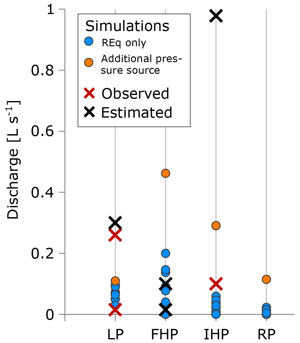
Figure 9Simulated, observed (measured) and estimated (“by eye”) spring discharge rates. Blue dots are discharge rates simulated for groundwater model scenarios for which the source term is defined by the rate of basal permafrost aggradation (Figs. 7 and 8). The orange dots are discharge rates simulated for a groundwater model scenario with an additional unknown pressure source (Fig. 10).
In Fig. 9, simulated spring outflows from all model simulations are plotted together with the few available observations. Validation of any particular model scenario was not possible due to the variability and paucity of observations. Nevertheless, assuming that only a small fraction of the discharge (if any) freezes within the pingo and becomes part of its core, the comparable observed and simulated discharges suggest that permafrost aggradation alone may explain the presence of the pingos and their springs in low-permeability systems comparable to the one modelled. To investigate the effect of additional pressure sources, we ran the groundwater model with maximum K values (Table 3) and different, uniformly distributed recharge rates, all resulting in a greater total inflow of groundwater than from permafrost aggradation alone (Fig. 8). We used the maximum K values to allow for the highest amount of recharge to enter the system. Figure 10 illustrates such a scenario with a recharge rate of 1 mm yr−1. We found that, if the pressure production exceeds that equivalent to a recharge rate of 1 mm yr−1, hydraulic heads rise unrealistically (i.e. >200 m a.g.l.). Within the model limitations (Sect. 6.2), Fig. 10 may thus be regarded as an approximation of the upper limit of possible total inflow (or pore space loss) rates (161.4 m3 d−1). The corresponding spring water discharge rates range from 0.12 to 0.56 L s−1 (Fig. 9), and the mean residence time is 24 kyr.
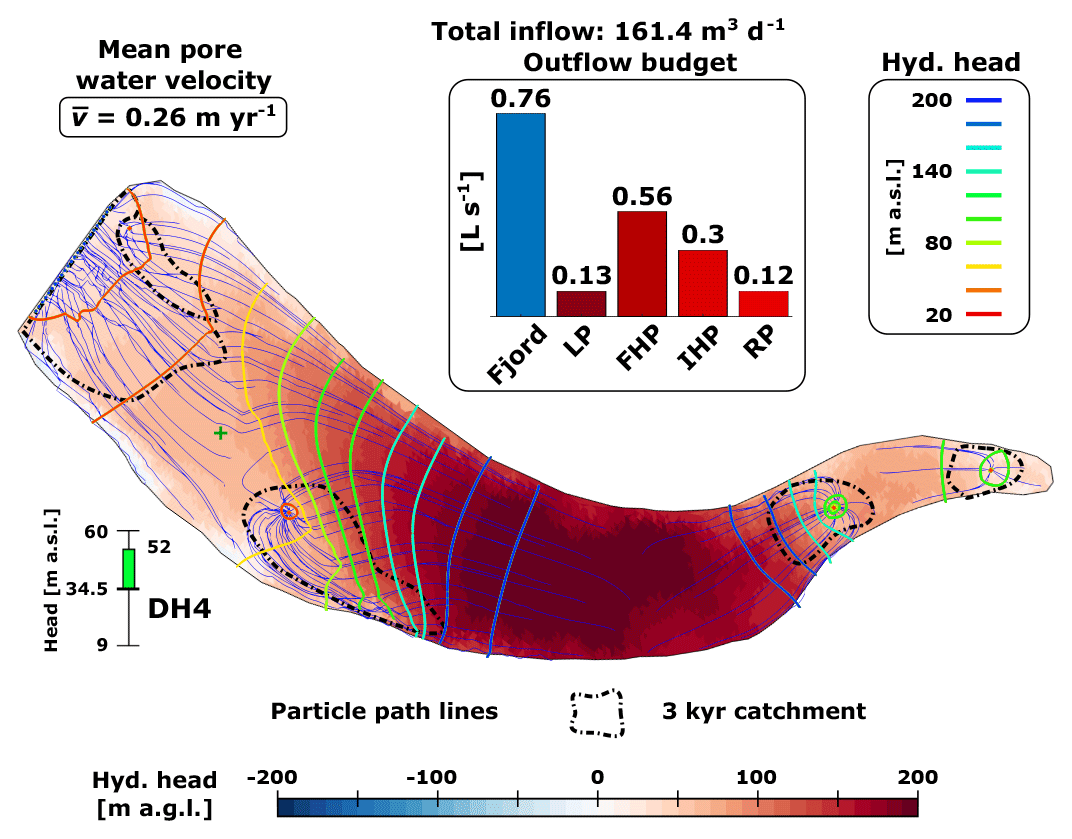
Figure 10Groundwater model simulation representing additional pressure sources. Recharge is distributed uniformly at a rate of 1 mm yr−1. This figure uses the same structure and legend as Fig. 8.
6.4 Comparison with hydrological processes inferred from pingo spring water chemistry
The lack of hydrological data for model calibration makes a comparison with other information on the groundwater system ever so important. In this context, hydrochemical data from 25 pingo spring water samples from 2014 to 2017 (Hodson et al., 2020; see https://doi.org/10.5285/3d82fd3f-884b-47b6-b11c-6c96d66b950d) give additional insights into the groundwater system. Accordingly, water samples from Lagoon Pingo (LP), FHP, Innerhytte Pingo (IHP) and River Pingo (RP) reveal that all these pingo springs share the same sodium bicarbonate (NaHCO3) water type (illustrated in the Supplement) which is commonly associated with freshening of a saline groundwater system (e.g. Giménez-Forcada, 2010). The only exceptions are four samples taken near River Pingo in 2017 which are of a magnesium sulfate water type. These four samples were excluded from the following discussion because they might not be associated with a pingo according to Hodson et al. (2020).

Figure 11Cl− concentration and of pingo spring water samples. The thick black model line is drawn by assuming that the LP samples result from the mixing of seawater and a freshwater endmember with a zero Cl− concentration. The range of possible values following freeze-out (Eq. 8) from water with an initial composition similar to LP is illustrated with the shaded area. Here, Cl− is assumed to be completely excluded from the ice. The lower and upper edges of the shading represent equilibrium fractionation and no fractionation, respectively, while the intermediate model lines illustrate fractionation at 20 %, 40 %, 60 % and 80 % (top–bottom) of equilibrium conditions.
Among the 21 NaHCO3-dominated samples, a few distinct trends were observed in the hydrochemistry. Specifically, the concentration of Cl− and heavy stable water isotopes both increase in the up-valley direction. To illustrate this, the concentration of Cl− is plotted against in Fig. 11. The former has a relatively constant concentration at each site compared to the latter. We inferred that the variation in the Cl− concentrations between the different springs reflects an up-valley variation in the sub-permafrost groundwater system and not processes acting locally along the flow paths towards the individual pingos. If the latter had been the case, we would expect to see greater intra-site variation.
In order to explain the increasing Cl− concentration and , we considered solute rejection and isotope fractionation associated with freezing, as well as mixing between seawater and freshwater. For the former, we found that the positive relationship between the two parameters was incongruent with this being a major control in the investigated system: when ice forms, water molecules containing the heavier isotope 18O (and D) are preferentially included in the ice, while the residual water becomes isotopically lighter. For freezing in a well-mixed and closed reservoir, the isotopic ratio in the residual water, δw, may be expressed by a Rayleigh-type fractionation according to the following equation: (Lacelle, 2011):
where δ0 is the initial isotopic ratio in the water, αi−w is the fractionation coefficient between ice and water, and f is the fraction of residual water. At equilibrium, (Lehmann and Siegenthaler, 1991), and it approaches 1 for faster freezing rates (non-equilibrium). The decrease in in the residual water resulting from freezing is exemplified in Fig. 11 by taking a typical LP water sample (i.e. with the lowest salinity) and assuming that Cl− is completely excluded from the ice. The shading indicates the possible range of that can be derived from this process. Although two samples from FHP fall within the shaded area, it was hard to explain the composition of these with freezing from an LP-type water as the remaining samples did not comply with this interpretation (Fig. 11).
Another model line in Fig. 11 is drawn by assuming that the LP samples result from the mixing of seawater and a freshwater endmember with zero Cl− concentration. Generally, the remaining samples agree with this model line, and hence we argue that mixing is the more feasible explanation. This was also in line with the interpretation that the NaHCO3-dominated hydrochemistry reflects freshening.
For the above mixing scenario, field surveys suggested a somewhat unusual trend with greater fractions of freshwater towards the sea, where and Cl− concentrations approach those of the inferred freshwater endmember in Fig. 11. In the case of present-day recharge from the adjacent mountains (as demonstrated at a pingo 35 km south-west of Adventdalen by Demidov et al., 2019), we would not expect to observe such a systematic trend along the valley axis as this would be unlikely in a system dependent upon localised areas for infiltration. We therefore suggest that the unexpected landwards increase in Cl− is difficult to explain without the sequence of events illustrated in Fig. 12. During glaciation, the groundwater system was recharged by subglacial melting (Fig. 12a). Despite being covered by the sea during the Early Holocene, seawater could not infiltrate substantially into the groundwater system to replace the fresh groundwater (Fig. 12b). In Fig. 12c, the body of freshwater forms a wedge that thins inland below the freezing front due to the density difference with seawater. Moving away from the sea, the springs expel more saline groundwater because the wedge thins in this direction and the permafrost thickness increases (Fig. 12c). Therefore, both the sources of water and the hydraulic conditions of the groundwater system seem intricately linked to landscape evolution throughout the Holocene.
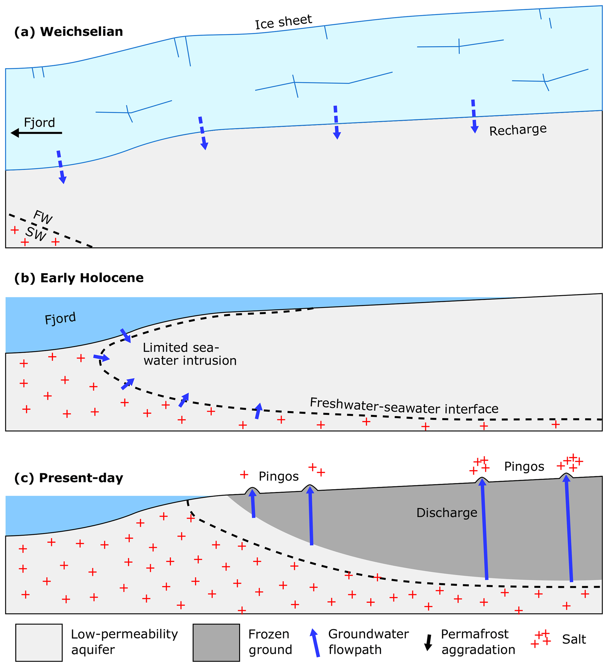
Figure 12Possible interpretation of hydrochemical trends observed in pingo spring waters. (a) Subglacial melting from the Weichselian ice sheet recharged the groundwater system with freshwater. (b) Although covered by the sea during the Early Holocene, low-permeability rocks limited infiltration of seawater, and the fresh groundwater body persisted. (c) Due to the shallower permafrost depth towards the sea, spring water sampled in this direction holds a lower concentration of seawater (salt).
6.5 Pan-Arctic significance
The hydrological system proposed here, in which time-transgressive basal permafrost aggradation in an uplifted Arctic valley is able to drive the flow of deep groundwater to the surface, may at first appear unusual. However, the combination of Holocene marine regression and climate cooling, which have resulted in this system, is neither unique to Adventdalen nor to Svalbard. As exemplified by Holocene temperatures on Svalbard (Fig. 3), a general climate cooling from the Holocene thermal maximum to the pre-industrial age occurred throughout the Arctic (Kaufman et al., 2020). Marine regression took place where the rate of postglacial rebound or sediment supply surpassed the Holocene eustatic sea level rise (Kidson and Heyworth, 1978). Virtually all valleys on Svalbard and Greenland located close to sea level have been exposed to such a postglacial rebound (Ingólfsson and Landvik, 2013; Weidick and Bennike, 2007), and other examples are found in the Canadian High Arctic (Aitken and Gilbert, 1989; Bell, 1996; Lemmen et al., 1994). Considering the frequency of these fundamental conditions required for the proposed mechanism, we suggest that millennial-scale permafrost aggradation may also drive the flow of sub-permafrost groundwater to the surface in other uplifted Arctic valleys.
Results from the decoupled heat and groundwater model show that millennial-scale basal permafrost aggradation may alone produce hydraulic pressures sufficient for the formation of pingos and their spring water outflows when the right conditions are met. In addition to the climate cooling necessary for permafrost aggradation, a relatively low-permeability groundwater system with limited dissipation of hydraulic pressures is also required for pingo formation. Pingos formed in this way do not conform to the traditional differentiation between open-system and closed-system types but constitute a borderline case: by definition, they are classified as open-system pingos because the groundwater body from which spring water is expelled is not enclosed in permafrost. Generically, though, they relate more to closed-system pingos because the causal mechanism of hydraulic pressures is essentially similar, although operating over much longer timescales. We emphasise that this conceptual model for pingo formation represents an endmember of open-system pingo-forming processes which is not exclusive but may act in combination with others, such as those reported nearby by Demidov et al. (2019).
The simulation results from the 1DHT model suggested that basal permafrost aggradation in Adventdalen presently induces head gradients corresponding to the effect of a recharge rate of ∼0.1 mm yr−1 furthest up-valley and increasing to ∼1 mm yr−1 towards the sea. By applying these rates to the groundwater model, we simulated spring outflow rates on the order of 10−1 L s−1. Due to the probable occurrence of basal permafrost aggradation outside the model area, these may be underestimations. Nevertheless, the simulated and observed spring outflow rates at Adventdalen pingos were of the same order of magnitude, suggesting that they likely form at least partly in accordance with our conceptual model. This further suggests that overpressures induced by water expansion during freezing in other sub-permafrost groundwater systems can result from permafrost aggradation.
The simulated aquifer flow paths and flow velocity distributions suggested that sub-permafrost groundwater flow in Adventdalen is characterised by slow mean pore water velocities (<0.25 m yr−1) and long residence times ( years) that exceed the duration of the Holocene. The groundwater system most likely has a multidirectional flow pattern with individual catchments around each pingo.
Alternative and non-recharge-related processes that may also affect sub-permafrost pressures were considered. The role of gases may be particularly important in this context because it is likely that methane hydrates have influenced the groundwater system under investigation. However, methane hydrate dissolution may in fact act as a pressure buffer and prolong artesian pressures after permafrost ceases aggrading (or starts thawing). This represents an uncertainty in forecasting how groundwater and methane fluxes will react to climate change. Unresolved questions regarding the occurrence and formation of gases in sub-permafrost groundwater systems therefore constitute an ongoing challenge for Arctic science.
The presence of a positive relationship between Cl− and in the pingo spring water samples suggests that mixing between seawater and freshwater is the major control of hydrogeochemistry in the sub-permafrost groundwater system prior to aggradation. As a result, a somewhat unexpected but clear trend of increasing salinity in an up-valley direction was found. Therefore, given the relatively stagnant groundwater system, Weichselian subglacial meltwater could endure the Early Holocene inundation and result in the present-day situation in which a freshwater body forms a wedge that thins in the inland direction below the permafrost. This possible interpretation readily explains the inland increase in the spring salinity because the inland springs expel groundwater from greater and hence more saline depths.
To our knowledge, this is the first study to show that time-transgressive basal permafrost aggradation in an uplifted Arctic valley represents a feasible mechanism for driving the flow of deep groundwater to the surface, and so the hydrological system in Adventdalen might appear unusual at first. However, considering that isostatic uplift in permafrost valley systems is common across the Arctic, millennial-scale permafrost aggradation deserves more attention as a driver of sustained gas and groundwater flows from the sub-permafrost environment to the land surface.
The 1DHT model code is publicly available at https://doi.org/10.5281/zenodo.4240594 (Hornum, 2020).
The supplement related to this article is available online at: https://doi.org/10.5194/tc-14-4627-2020-supplement.
MTH developed the 1DHT model code and designed the modelling experiments with contributions from VB. AJH, SJ and MTH analysed the hydrochemical data. MTH developed the geological model with contributions from KS. MTH prepared the paper with contributions from all the co-authors.
The authors declare that they have no conflict of interest.
This paper largely emanated from work initiated in Mikkel Toft Hornum's MSc thesis (Hornum, 2018), and the authors acknowledge Peter Engesgaard for supervising the thesis work. The authors are grateful to the editor and reviewers, whose constructive feedback and comments were very helpful for improving this paper.
This research has been supported by the The Research Council of Norway (grant no. 294764).
This paper was edited by Peter Morse and reviewed by Melissa Bunn and one anonymous referee.
Åhman, R.: Studier av pingoer i Adventdalen och Reindalen på Spetsbergen, Lunds Univ. Naturgeografiska Institution, Rapp. och Not., 15, 27–44, 1973.
Aitken, A. E. and Gilbert, R.: Holocene Nearshore Environments and Sea-Level History in Pangnirtung Fiord, Baffin Island, N.W.T., Canada, Arctic Alppine Res., 21, 34–44, 1989.
Andersen, D. T., Pollard, W. H., McKay, C. P., and Heldmann, J.: Cold springs in permafrost on Earth and Mars, J. Geophys. Res.-Planets, 107, 5015, https://doi.org/10.1029/2000je001436, 2002.
AQUAVEO™: Groundwater Modeling System 10.4.4, available at: https://www.aquaveo.com/software/gms-groundwater-modeling-system-introduction, last access: 1 December 2019.
Bælum, K., Johansen, T. A., Johnsen, H., Rød, K., Ruud, B. O., and Braathen, A.: Subsurface structures of the Longyearbyen CO2 Lab study area in Central Spitsbergen (Arctic Norway) as mapped by reflection seismic data, Nor. Geol. Tidsskr., 92, 377–389, 2012.
Bahr, J. M., Moline, G. R., and Nadon, G. C.: Anomalous Pressures in the Deep Michigan Basin, AAPG Memoir., 61, 153–165, 1994.
Ballantyne, C. K.: Periglacial geomorphology, 1st edn., John Wiley and Sons, West Sussex, UK, 2018.
Bell, T.: The last glaciation and sea level history of Fosheim Peninsula, Ellesmere Island, Canadian High Arctic, Can. J. Earth Sci., 33, 1075–1086, https://doi.org/10.1139/e96-082, 1996.
Benn, D. I. and Evans, D. J. A.: Glaciers and Glaciation, 2nd ed., Hodder Education, London, UK, 2010.
Bense, V. F., Kooi, H., Ferguson, G., and Read, T.: Permafrost degradation as a control on hydrogeological regime shifts in a warming climate, J. Geophys. Res.-Earth, 117, 1–18, https://doi.org/10.1029/2011JF002143, 2012.
Bergman, T. L., Lavine, A. S., Incropera, F. P., and Dewitt, D. P.: Fundamentals of Heat and Mass Transfer, 7th edn., John Wiley and Sons, West Sussex, UK, 2011.
Betlem, P., Senger, K., and Hodson, A.: 3D thermobaric modelling of the gas hydrate stability zone onshore central Spitsbergen, Arctic Norway, Mar. Pet. Geol., 100, 246–262, https://doi.org/10.1016/j.marpetgeo.2018.10.050, 2019.
Birchall, T., Senger, K., Hornum, M. T., Olaussen, S., and Braathen, A.: Underpressure of the Northern Barents Shelf: distribution, causes and implications on the petroleum, Pre-proof, Am. Assoc. Pet. Geol. Bull., 104, 2267–2295, https://doi.org/10.1306/02272019146, 2020.
Bonacina, C. and Comini, G.: On the solution of the nonlinear heat conduction equations by numerical methods, Int. J. Heat Mass Transf., 16, 581–589, https://doi.org/10.1016/0017-9310(73)90225-1, 1973.
Braathen, A., Bælum, K., Christiansen, H. H., Dahl, T., Eiken, O., Elvebakk, H., Hansen, F., Hanssen, T. H., Jochmann, M., Johansen, T. A., Johnsen, H., Larsen, L., Lie, T., Mertes, J., Mørk, A., Mørk, M. B., Nemec, W., Olaussen, S., Oye, V., Rød, K., Titlestad, G. O., Tveranger, J., and Vagle, K.: The Longyearbyen CO2 Lab of Svalbard, Norway – Initial Assessment of the Geological Conditions for CO2 Sequestration, Nor. Geol. Tidsskr., 92, 353–376, 2012.
Burland, J. B.: On the compressibility and shear strength of natural clays, Géotecnique, 40, 329–378, 1990.
Burr, D. M., Tanaka, K. L., and Yoshikawa, K.: Pingos on Earth and Mars, Planet. Space Sci., 57, 541–555, https://doi.org/10.1016/j.pss.2008.11.003, 2009.
Burt, T. P. and Williams, P. J.: Hydraulic conductivity in frozen soils, Earth Surf. Process., 1, 349–360, https://doi.org/10.1002/esp.3290010404, 1976.
Cable, S., Elberling, B., and Kroon, A.: Holocene permafrost history and cryostratigraphy in the High-Arctic Adventdalen Valley, central Svalbard, Boreas, 47, 423–442, https://doi.org/10.1111/bor.12286, 2018.
Carslaw, H. S. and Jaeger, J. C.: Conduction of heat in solids, 2nd ed., Clarendon Press, London, UK, 1959.
Christiansen, H. H., French, H. M., and Humlum, O.: Permafrost in the Gruve-7 mine, Adventdalen, Svalbard, Nor. Geogr. Tidsskr., 59, 109–115, https://doi.org/10.1080/00291950510020592, 2005.
Demidov, N., Wetterich, S., Verkulich, S., Ekaykin, A., Meyer, H., Anisimov, M., Schirrmeister, L., Demidov, V., and Hodson, A. J.: Geochemical signatures of pingo ice and its origin in Grøndalen, west Spitsbergen, The Cryosphere, 13, 3155–3169, https://doi.org/10.5194/tc-13-3155-2019, 2019.
Domenico, P. A. and Mifflin, M. D.: Water from low-permeability sediments and land subsidence, Water Resour. Res., 1, 563–576, https://doi.org/10.1029/WR001i004p00563, 1965.
Domenico, P. A. and Schwartz, F. W.: Physical and chemical hydrogeology, John Wiley and Sons, New York, NY, USA, 1998.
Dyke, A. S., England, J., Reimnitz, E., and Jette, H.: Changes in driftwood delivery to the Canadian Arctic Archipelago, Arctic, 50, 1–16, 1997.
Elverhøi, A., Svendsen, J. I., Solheim, A., Andersen, E. S., Milliman, J., Mangerud, J., and Hooke, R. L.: Late Quaternary Sediment Yield from the High Arctic Svalbard Area, J. Geol., 103, 1–17, https://doi.org/10.1086/629718, 1995.
Eppelbaum, L., Kutasov, I., and Pilchin, A.: Paleoclimate and Present Climate Warming Trends, in: Applied Geothermics, Lecture Notes in Earth System Sciences, 655–693, Springer, Berlin, Heidelberg, Germany, https://doi.org/10.1007/978-3-642-34023-9_11, 2014.
Farnsworth, W. R., Ingólfsson, Ó., Alexanderson, H., Allaart, L., Forwick, M., Noormets, R., Retelle, M., and Schomacker, A.: Holocene glacial history of Svalbard: Status, perspectives and challenges, Earth-Sci. Rev., 208, 103249, https://doi.org/10.1016/j.earscirev.2020.103249, 2020.
Fitts, C. R.: Groundwater Science, 1st edn., Academic Press, London, UK, 2002.
Førland, E. J., Hanssen-Bauer, I., and Nordli, Ø.: Climate statistics and longterm series of temperature and precipitation at Svalbard and Jan Mayen, DNMI Nor. Meteorol. Inst. Rep. 21, Norwegian Meteorological Institute, Oslo, Norway, 72, 1997.
Forman, S. L.: Post-glacial relative sea-level history of northwestern Spitsbergen, Svalbard, Geol. Soc. Am. Bull., 102, 1580–1590, https://doi.org/10.1130/0016-7606(1990)102<1580:PGRSLH>2.3.CO;2, 1990.
Forwick, M. and Vorren, T. O.: Stratigraphy and deglaciation of the Isfjorden area, Spitsbergen, Nor. Geol. Tidsskr., 90, 163–179, 2011.
French, H. M.: The Periglacial Environment, 4th ed., John Wiley and Sons, West Sussex, UK, 2017.
Funder, S., Goosse, H., Jepsen, H., Kaas, E., Kjær, K. H., Korsgaard, N. J., Larsen, N. K., Linderson, H., Lyså, A., Möller, P., Olsen, J., and Willerslev, E.: A 10,000-Year Record of Arctic Ocean Sea-Ice Variability – View from the Beach, Science, 333, 747–750, https://doi.org/10.1126/science.1202760, 2011.
Gilbert, G. L., O'Neill, H. B., Nemec, W., Thiel, C., Christiansen, H. H., and Buylaert, J. P.: Late Quaternary sedimentation and permafrost development in a Svalbard fjord-valley, Norwegian high Arctic, Sedimentology, 65, 2531–2558, https://doi.org/10.1111/sed.12476, 2018.
Giménez-Forcada, E.: Dynamic of sea water interface using hydrochemical facies evolution diagram, Ground Water, 48, 212–216, https://doi.org/10.1111/j.1745-6584.2009.00649.x, 2010.
Govaerts, J., Beerten, K., and ten Veen, J.: Weichselian permafrost depth in the Netherlands: a comprehensive uncertainty and sensitivity analysis, The Cryosphere, 10, 2907–2922, https://doi.org/10.5194/tc-10-2907-2016, 2016.
Grasby, S. E., Beauchamp, B., and Bense, V.: Sulfuric Acid Speleogenesis Associated with a Glacially Driven Groundwater System – Paleo-spring “Pipes” at Borup Fiord Pass, Nunavut, Astrobiology, 12, 19–28, https://doi.org/10.1089/ast.2011.0700, 2012.
Grasby, S. E., Proemse, B. C., and Beauchamp, B.: Deep groundwater circulation through the High Arctic cryosphere forms Mars-like gullies, Geology, 42, 651–654, https://doi.org/10.1130/G35599.1, 2014.
Gregersen, O. and Eidsmoen, T.: Permafrost conditions in the shore area at Svalbard, in: Proceedings of the Fifth International Conference on Permafrost, Trondheim, Norway, 2–5 August 1988, 933–936, 1988.
Grenier, C., Anbergen, H., Bense, V., Chanzy, Q., Coon, E., Collier, N., Costard, F., Ferry, M., Frampton, A., Frederick, J., Gonçalvès, J., Holmén, J., Jost, A., Kokh, S., Kurylyk, B., McKenzie, J., Molson, J., Mouche, E., Orgogozo, L., Pannetier, R., Rivière, A., Roux, N., Rühaak, W., Scheidegger, J., Selroos, J. O., Therrien, R., Vidstrand, P., and Voss, C.: Groundwater flow and heat transport for systems undergoing freeze-thaw: Intercomparison of numerical simulators for 2D test cases, Adv. Water Resour., 114, 196–218, https://doi.org/10.1016/j.advwatres.2018.02.001, 2018.
Grosse, G., Goetz, S., McGuire, A. D., Romanovsky, V. E., and Schuur, E. A. G.: Changing permafrost in a warming world and feedbacks to the Earth system, Environ. Res. Lett., 11, 040201, https://doi.org/10.1088/1748-9326/11/4/040201, 2016.
Grundvåg, S.-A., Jelby, M. E., Sliwinska, K. K., Nøhr-Hansen, H., Aadland, T., Sandvik, S. E., Tennvassås, I., Engen, T., and Olaussen, S.: Sedimentology and palynology of the Lower Cretaceous succession of central Spitsbergen: integration of subsurface and outcrop data, Nor. J. Geol., 99, 253–284, https://doi.org/10.17850/njg006, 2019.
Hald, M., Andersson, C., Ebbesen, H., Jansen, E., Klitgaard-Kristensen, D., Risebrobakken, B., Salomonsen, G. R., Sarnthein, M., Sejrup, H. P., and Telford, R. J.: Variations in temperature and extent of Atlantic Water in the northern North Atlantic during the Holocene, Quaternary Sci. Rev., 26, 3423–3440, https://doi.org/10.1016/j.quascirev.2007.10.005, 2007.
Haldorsen, S., Heim, M., and Lauritzen, S. E.: Subpermafrost Groundwater, Western Svalbard, Nord. Hydrol., 27, 57–68, https://doi.org/10.2166/nh.1996.0019, 1996.
Haldorsen, S., Heim, M., Dale, B., Landvik, J. Y., van der Ploeg, M., Leijnse, A., Salvigsen, O., Hagen, J. O., and Banks, D.: Sensitivity to long-term climate change of subpermafrost groundwater systems in Svalbard, Quaternary Res., 73, 393–402, https://doi.org/10.1016/j.yqres.2009.11.002, 2010.
Hanssen-Bauer, I., Førland, E. J., Hisdal, H., Mayer, S., Sandø, A. B., Sorteberg, A., Adakudlu, M., Andresen, J., Bakke, J., Beldring, S., Benestad, R., Bilt, W., Bogen, J., Borstad, C., Breili, K., Breivik, Ø., Børsheim, K. Y., Christiansen, H. H., Dobler, A., Engeset, R., Frauenfelder, R., Gerland, S., Gjelten, H. M., Gundersen, J., Isaksen, K., Jaedicke, C., Kierulf, H., Kohler, J., Li, H., Lutz, J., Melvold, K., Mezghani, A., Nilsen, F., Nilsen, I. B., Nilsen, J. E. Ø., Pavlova, O., Ravndal, O., Risebrobakken, B., Saloranta, T., Sandven, S., Schuler, T. V, Simpson, M. J. R., Skogen, M., Smedsrud, L. H., Sund, M., Vikhamar-Schuler, D., Westermann, S., and Wong, W. K.: Climate in Svalbard 2100 – a knowledge base for climate adaption, Norwegian Centre for Climate Services Report 1/2019, Norwegian Environment Agency, Trondheim, Norway, 105, 2019.
Harada, K. and Yoshikawa, K.: Permafrost age and thickness near Adventfjorden, Spitsbergen, Polar Geogr., 20, 267–281, https://doi.org/10.1080/10889379609377607, 1996.
Hodson, A., Nowak, A., Redeker, K. R., Holmlund, E. S., Christiansen, H. H., and Turchyn, A. V.: Seasonal Dynamics of Methane and Carbon Dioxide Evasion From an Open System Pingo: Lagoon Pingo, Svalbard, Front. Earth Sci., 7, 30, https://doi.org/10.3389/feart.2019.00030, 2019.
Hodson, A. J., Nowak, A., Hornum, M. T., Senger, K., Redeker, K., Christiansen, H. H., Jessen, S., Betlem, P., Thornton, S. F., Turchyn, A. V., Olaussen, S., and Marca, A.: Sub-permafrost methane seepage from open-system pingos in Svalbard, The Cryosphere, 14, 3829–3842, https://doi.org/10.5194/tc-14-3829-2020, 2020.
Hornum, M. T.: Postglacial Rebound, Permafrost Growth, and its Impact on Groundwater Flow and Pingo Formation, University of Copenhagen, available at: https://researchinsvalbard.no/project/8729 (last access: 16 December 2020), 2018.
Hornum, M. T.: mikkeltoft/-1DHT-model-code: 1DHT model code v1.0 (Version v1.1), Zenodo, https://doi.org/10.5281/zenodo.4240594, 2020.
Humlum, O.: Holocene permafrost aggradation in Svalbard, Geol. Soc. Spec. Publ., 242, 119–130, https://doi.org/10.1144/GSL.SP.2005.242.01.11, 2005.
Humlum, O., Instanes, A., and Sollid, J. L.: Permafrost in Svalbard: A review of research history, climatic background and engineering challenges, Polar Res., 22, 191–215, https://doi.org/10.3402/polar.v22i2.6455, 2003.
Huq, F., Smalley, P. C., Mørkved, P. T., Johansen, I., Yarushina, V., and Johansen, H.: The Longyearbyen CO2 Lab: Fluid communication in reservoir and caprock, Int. J. Greenh. Gas Control, 63, 59–76, https://doi.org/10.1016/j.ijggc.2017.05.005, 2017.
Ingólfsson, Ó. and Landvik, J. Y.: The Svalbard–Barents Sea ice-sheet – Historical, current and future perspectives, Quaternary Sci. Rev., 64, 33–60, https://doi.org/10.1016/j.quascirev.2012.11.034, 2013.
Kaufman, D., McKay, N., Routson, C., Erb, M., Dätwyler, C., Sommer, P. S., Heiri, O., and Davis, B.: Holocene global mean surface temperature, a multi-method reconstruction approach, Sci. Data, 7, 1–13, https://doi.org/10.1038/s41597-020-0530-7, 2020.
Kidson, C. and Heyworth, A.: Holocene eustatic sea level change, Nature, 273, 748–750, https://doi.org/10.1038/273748a0, 1978.
Koevoets, M. J., Hammer, Ø., Olaussen, S., Senger, K., and Smelror, M.: Integrating subsurface and outcrop data of the Middle Jurassic to Lower Cretaceous Agardhfjellet Formation in central Spitsbergen, Nor. J. Geol., 98, 1–34, https://doi.org/10.17850/njg98-4-01, 2018.
Kottek, M., Grieser, J., Beck, C., Rudolf, B., and Rubel, F.: World Map of the Köppen-Geiger climate classification updated, Meteorol. Z., 15, 259–263, https://doi.org/10.1127/0941-2948/2006/0130, 2006.
Lacelle, D.: On the δ18O, δD and D-excess relations in meteoric precipitation and during equilibrium freezing: Theoretical approach and field examples, Permafr. Periglac. Process., 22, 13–25, https://doi.org/10.1002/ppp.712, 2011.
Lehmann, M. and Siegenthaler, U.: Equilibrium oxygen- and hydrogen-isotope fractionation between ice and water, J. Glaciol., 37, 23–26, https://doi.org/10.3189/s0022143000042751, 1991.
Leith, K., Moore, J. R., Amann, F., and Loew, S.: Subglacial extensional fracture development and implications for Alpine Valley evolution, J. Geophys. Res.-Earth, 119, 62–81, https://doi.org/10.1002/2012JF002691, 2014.
Lemmen, D. S., Aitken, A. E., and Gilbert, R.: Early Holocene deglaciation of Expedition and Strand fiords, Canadian High Arctic, Can. J. Earth Sci., 31, 943–958, https://doi.org/10.1139/e94-084, 1994.
Liestøl, O.: Pingos, springs, and permafrost in Spitsbergen, Nor. Polarinstitutt Årb., 1975, 7–29, 1977.
Liestøl, O.: Open-system pingos in Spitsbergen, Nor. Geogr. Tidsskr., 50, 81–84, https://doi.org/10.1080/00291959608552355, 1996.
Lønne, I. and Nemec, W.: High-arctic fan delta recording deglaciation and environment disequilibrium, Sedimentology, 51, 553–589, https://doi.org/10.1111/j.1365-3091.2004.00636.x, 2004.
Mackay, J. R.: Pingo Growth and collapse, Tuktoyaktuk Peninsula Area, Western Arctic Coast, Canada: a long-term field study, Geogr. Phys. Quat., 52, 271–323, https://doi.org/10.7202/004847ar, 1998.
Manger, G. E.: Porosity and Bulk Density of Sedimentary Rocks, US Geological Survey Bulletin 1144-E, US Government Printing Office, Washington D.C., USA, 60, https://doi.org/10.3133/b1144E, 1963.
Mangerud, J. and Svendsen, J. I.: The Holocene Thermal Maximum around Svalbard, Arctic North Atlantic, molluscs show early and exceptional warmth, Holocene, 28, 65–83, https://doi.org/10.1177/0959683617715701, 2017.
Marshall, C., Uguna, J., Large, D. J., Meredith, W., Jochmann, M., Friis, B., Vane, C., Spiro, B. F., Snape, C. E., and Orheim, A.: Geochemistry and petrology of palaeocene coals from Spitzbergen – Part 2: Maturity variations and implications for local and regional burial models, Int. J. Coal Geol., 143, 1–10, https://doi.org/10.1016/j.coal.2015.03.013, 2015.
MathWorks: MATLAB R2019b, available at: https://se.mathworks.com/products/matlab.html, last access: 1 December 2019.
Mau, S., Römer, M., Torres, M. E., Bussmann, I., Pape, T., Damm, E., Geprägs, P., Wintersteller, P., Hsu, C. W., Loher, M., and Bohrmann, G.: Widespread methane seepage along the continental margin off Svalbard – from Bjørnøya to Kongsfjorden, Sci. Rep.-UK, 7, 42997, https://doi.org/10.1038/srep42997, 2017.
McCauley, C. A., White, D. M., Lilly, M. R., and Nyman, D. M.: A comparison of hydraulic conductivities, permeabilities and infiltration rates in frozen and unfrozen soils, Cold Reg. Sci. Technol., 34, 117–125, https://doi.org/10.1016/S0165-232X(01)00064-7, 2002.
McDonald, M. G. and Harbaugh, A. W.: A modular three-dimensional finite-difference ground-water flow model, Techniques of Water-Resources Investigations 06-A1, US Geological Survey, Reston, VA, USA, 586, https://doi.org/10.3133/twri06A1, 1988.
Mottaghy, D. and Rath, V.: Latent heat effects in subsurface heat transport modelling and their impact on palaeotemperature reconstructions, Geophys. J. Int., 164, 236–245, https://doi.org/10.1111/j.1365-246X.2005.02843.x, 2006.
Myhre, C. L., Ferré, B., Platt, S. M., Silyakova, A., Hermansen, O., Allen, G., Pisso, I., Schmidbauer, N., Stohl, A., Pitt, J., Jansson, P., Greinert, J., Percival, C., Fjaeraa, A. M., O'Shea, S. J., Gallagher, M., Le Breton, M., Bower, K. N., Bauguitte, S. J. B., Dalsøren, S., Vadakkepuliyambatta, S., Fisher, R. E., Nisbet, E. G., Lowry, D., Myhre, G., Pyle, J. A., Cain, M., and Mienert, J.: Extensive release of methane from Arctic seabed west of Svalbard during summer 2014 does not influence the atmosphere, Geophys. Res. Lett., 43, 4624–4631, https://doi.org/10.1002/2016GL068999, 2016.
Neuzil, C. E.: Abnormal pressures as hydrodynamic phenomena, Am. J. Sci., 295, 742–786, https://doi.org/10.2475/ajs.295.6.742, 1995.
Neuzil, C. E.: Hydromechanical coupling in geologic processes, Hydrogeol. J., 11, 41–83, https://doi.org/10.1007/s10040-002-0230-8, 2003.
Neuzil, C. E.: Hydromechanical effects of continental glaciation on groundwater systems, Geofluids, 12, 22–37, https://doi.org/10.1111/j.1468-8123.2011.00347.x, 2012.
Nordli, Ø., Przybylak, R., Ogilvie, A. E. J., and Isaksen, K.: Long-term temperature trends and variability on spitsbergen: The extended svalbard airport temperature series, 1898–2012, Polar Res., 33, 21349, https://doi.org/10.3402/polar.v33.21349, 2014.
Norwegian Polar Institute: Map data, available at: https://geodata.npolar.no/ (last access: 13 May 2020), 2019.
Ohm, S. E., Larsen, L., Olaussen, S., Senger, K., Birchall, T., Demchuk, T., Hodson, A., Johansen, I., Titlestad, G. O., Karlsen, D. A., and Braathen, A.: Discovery of shale gas in organic-rich Jurassic successions, Adventdalen, Central Spitsbergen, Norway, Nor. J. Geol., 99, 1–28, https://doi.org/10.17850/njg007, 2019.
Okiongbo, K. S.: Effective Stress-Porosity Relationship above and Within the Oil Window in the North Sea Basin, Res. J. Appl. Sci. Eng. Technol., 3, 32–38, 2011.
Olaussen, S., Senger, K., Braathen, A., Grundvåg, S.-A., and Mørk, A.: You learn as long as you drill, research synthesis from the Longyearbyen CO2 Laboratory, Svalbard, Norway, Nor. J. Geol., 99, 157–187, https://doi.org/10.17850/njg008, 2020.
Orvin, A. K.: Litt om kilder på Svalbard, Nor. Geol. Tidsskr., 10, 15–38, 1944.
Pollock, D. W.: User Guide for MODPATH Version 7-A Particle-Tracking Model for MODFLOW, Open File Rep., 1086, US Geological Survey, Reston, VA, USA, 41, https://doi.org/10.3133/ofr20161086, 2016.
Riseborough, D., Shiklomanov, N., Etzelmüller, B., Gruber, S., and Marchenko, S.: Recent advances in permafrost modelling, Permafr. Periglac. Process., 19, 137–156, https://doi.org/10.1002/ppp.615, 2008.
Robertson, E. C.: Thermal properties of rocks, Report 88-441, US Dep. Inter., US Geological Survey, Reston, VA, USA, 106, 1988.
Scheidegger, J. M. and Bense, V. F.: Impacts of glacially recharged groundwater flow systems on talik evolution, J. Geophys. Res.-Earth, 119, 758–778, https://doi.org/10.1002/2013JF002894, 2014.
Scheidegger, J. M., Bense, V. F., and Grasby, S. E.: Transient nature of Arctic spring systems driven by subglacial meltwater, Geophys. Res. Lett., 39, 1–6, https://doi.org/10.1029/2012GL051445, 2012.
Schlumberger©: Petrel E&P, available at: https://www.software.slb.com/products/petrel, last access: 1 December 2019.
Schuster, P. F., Schaefer, K. M., Aiken, G. R., Antweiler, R. C., Dewild, J. F., Gryziec, J. D., Gusmeroli, A., Hugelius, G., Jafarov, E., Krabbenhoft, D. P., Liu, L., Herman-Mercer, N., Mu, C., Roth, D. A., Schaefer, T., Striegl, R. G., Wickland, K. P., and Zhang, T.: Permafrost Stores a Globally Significant Amount of Mercury, Geophys. Res. Lett., 45, 1463–1471, https://doi.org/10.1002/2017GL075571, 2018.
Singhal, B. B. S. and Gupta, R. P.: Applied Hydrogeology of Fractured Rocks, 2nd ed., Springer, Dordrecht, the Netherlands, 2010.
Skempton, A. W.: The consolidation of clays by gravitational compaction, Q. J. Geol. Soc. London, 125, 373–408, https://doi.org/10.1144/gsjgs.125.1.0373, 1969.
Šuklje, L.: Rheologic Aspects of Soil Mechanics, 1st ed., Wiley-Interscience, London, UK, 1969.
Svensson, H.: Pingos i yttre delen av Adventdalen, Nor. Polarinstitutt Årb., 1969, 168–174, 1970.
Taniguchi, M.: Evaluations of the saltwater-groundwater interface from borehole temperature in a coastal region, Geophys. Res. Lett., 27, 713–716, https://doi.org/10.1029/1999GL002366, 2000.
van der Bilt, W. G. M., D'Andrea, W. J., Bakke, J., Balascio, N. L., Werner, J. P., Gjerde, M., and Bradley, R. S.: Alkenone-based reconstructions reveal four-phase Holocene temperature evolution for High Arctic Svalbard, Quaternary Sci. Rev., 183, 204–213, https://doi.org/10.1016/j.quascirev.2016.10.006, 2018.
van der Ploeg, M. J., Haldorsen, S., Leijnse, A., and Heim, M.: Subpermafrost groundwater systems: Dealing with virtual reality while having virtually no data, J. Hydrol., 475, 42–52, https://doi.org/10.1016/j.jhydrol.2012.08.046, 2012.
Verruijt, A.: A note on the Ghyben–Herzberg formula, Int. Assoc. Sci. Hydrol. Bull., 13, 43–46, https://doi.org/10.1080/02626666809493624, 1968.
Walvoord, M. A. and Kurylyk, B. L.: Hydrologic impacts of thawing permafrost – a review, Vadose Zone J., 15, 1–20, https://doi.org/10.2136/vzj2016.01.0010, 2016.
Wangen, M., Souche, A., and Johansen, H.: A model for underpressure development in a glacial valley, an example from Adventdalen, Svalbard, Basin Res., 28, 752–769, https://doi.org/10.1111/bre.12130, 2016.
Weidick, A. and Bennike, O.: Quaternary glaciation history and glaciology of Jakobshavn Isbræ and the Disko Bugt region, West Greenland: A review, Geol. Surv. Denmark Greenl. Bull., 14, 1–80, https://doi.org/10.34194/geusb.v14.4985, 2007.
Williams, J. R.: Ground Water in the Permafrost Regions of Alaska, USGS Prof. Paper 696, US Geological Survey, Reston, VA, USA, 90, https://doi.org/10.3133/pp696, 1970.
Williams, P. J. and Smith, M. W.: The Frozen Earth – Fundamentals of Geocryology, 1st edn., Cambridge University Press, New York, NY, USA, https://doi.org/10.1017/CBO9780511564437, 1989.
Woo, M. K.: Permafrost Hydrology, Springer, Berlin and Heidelberg, Germany, 2012.
Yang, Y. and Aplin, A. C.: Definition and practical application of mudstone porosity – effective stress relationships, Pet. Geosci., 10, 153–162, https://doi.org/10.1144/1354-079302-567, 2004.
Yoshikawa, K. and Harada, K.: Observations on nearshore pingo growth, Adventdalen, Spitsbergen, Permafr. Periglac. Process., 6, 361–372, https://doi.org/10.1002/ppp.3430060407, 1995.
Yoshikawa, K. and Nakamura, T.: Pingo growth ages in the delta area, Adventdalen, Spitsbergen, Polar Rec., 32, 347–352, https://doi.org/10.1017/S0032247400067565, 1996.