Frazil ice growth and production during katabatic wind events in the Ross Sea, Antarctica

Katabatic winds in coastal polynyas expose the ocean to extreme heat loss, causing intense sea ice production and dense water formation around Antarctica throughout autumn and winter. The advancing sea ice pack, combined with high winds and low temperatures, has limited surface ocean observations of polynyas in winter, thereby impeding new insights into the evolution of these ice factories through the dark austral months. Here, we describe oceanic observations during multiple katabatic wind events during May 2017 in the Terra Nova Bay and Ross Sea polynyas. Wind speeds regularly exceeded 20 m s⁻¹, air temperatures were below −25 ^∘C, and the oceanic mixed layer extended to 600 m. During these events, conductivity–temperature–depth (CTD) profiles revealed bulges of warm, salty water directly beneath the ocean surface and extending downwards tens of meters. These profiles reflect latent heat and salt release during unconsolidated frazil ice production, driven by atmospheric heat loss, a process that has rarely if ever been observed outside the laboratory. A simple salt budget suggests these anomalies reflect in situ frazil ice concentration that ranges from 13 to $\mathrm{266}\times {\mathrm{10}}^{-\mathrm{3}}$ kg m⁻³. Contemporaneous estimates of vertical mixing reveal rapid convection in these unstable density profiles and mixing lifetimes from 7 to 12 min. The individual estimates of ice production from the salt budget reveal the intensity of short-term ice production, up to 110 cm d⁻¹ during the windiest events, and a seasonal average of 29 cm d⁻¹. We further found that frazil ice production rates covary with wind speed and with location along the upstream–downstream length of the polynya. These measurements reveal that it is possible to indirectly observe and estimate the process of unconsolidated ice production in polynyas by measuring upper-ocean water column profiles. These vigorous ice production rates suggest frazil ice may be an important component in total polynya ice production.

1 Introduction

Latent heat polynyas form in areas where prevailing winds or oceanic currents create divergence in the ice cover, leading to openings either surrounded by extensive pack ice or bounded by land on one side and pack ice on the other (coastal polynyas) (Armstrong, 1972; Park et al., 2018). The open water of polynyas is critical for air–sea heat exchange, since ice-covered waters are better insulated and reduce the net heat flux to the atmosphere (Fusco et al., 2009; Talley et al., 2011). A key feature of coastal or latent heat polynyas are katabatic winds (Fig. 1), which form as cold, dense air masses over the ice sheets of Antarctica. These air masses flow as gravity currents, descending off the glacier, sometimes funneled by topography, as in the Terra Nova Bay polynya whose katabatic winds form in the Transantarctic Mountains. This episodic offshore wind creates and maintains latent heat polynyas. This study focuses on in situ measurements taken from two coastal latent heat polynyas in the Ross Sea, the Terra Nova Bay and the Ross Sea polynyas.

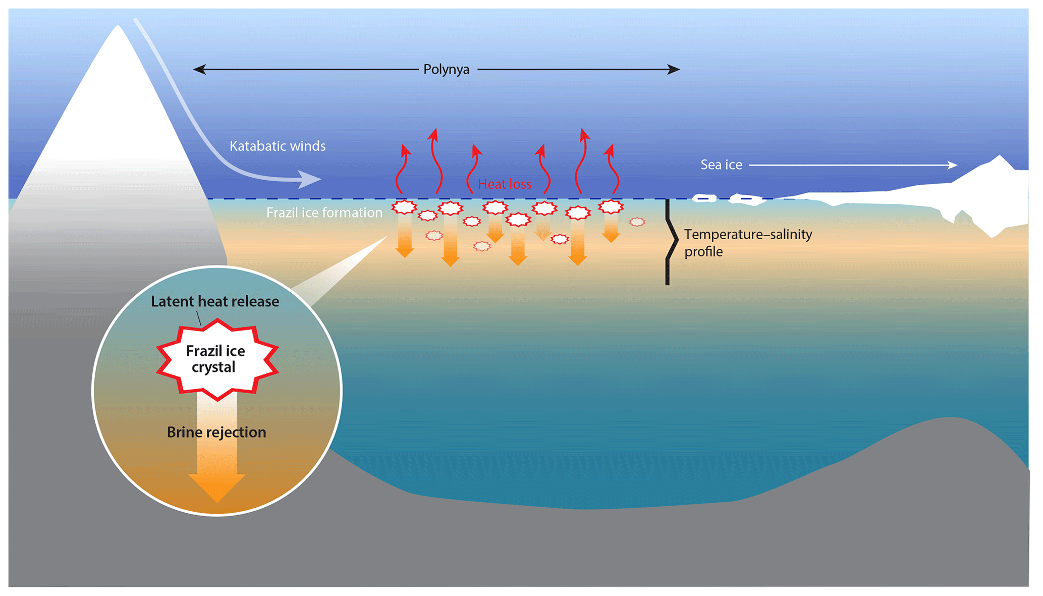
Figure 1 Schematic of a latent heat or coastal polynya. The polynya is kept open by katabatic winds which drive sea ice advection, oceanic heat loss, and frazil ice formation. Ice formation results in oceanic loss of latent heat to the atmosphere and brine rejection. The inset is a schematic of frazil ice formation that depicts the release of latent heat of fusion and brine rejection as a frazil ice crystal is formed.

Extreme oceanic heat loss in polynyas can generate supercooled water (colder than the freezing point; Skogseth et al., 2009; Dmitrenko et al., 2010; Matsumura and Ohshima, 2015), which is the precursor to ice nucleation. Ice formation begins with fine disc-shaped or dendritic crystals called frazil ice, which remain disaggregated when turbulent mixing is vigorous. These frazil ice crystals (Fig. 1 inset) are about 1 to 4 mm in diameter and 1–100 µm thick (Martin, 1981). In polynyas, frazil ice can mix vertically over a region of 5–15 m depth, while being transported downwind from the formation site (Heorton et al., 2017; Ito et al., 2015). Katabatic winds sustain the polynya by clearing frazil ice, which piles up at the polynya edge to form a consolidated ice cover (Morales Maqueda et al., 2004; Ushio and Wakatsuchi, 1993; Wilchinsky et al., 2015).

Brine rejection during ice crystal formation (Cox and Weeks, 1983) increases seawater salinity and density (Ohshima et al., 2016). In polynyas, this process is episodic and persistent over months, leading to the production of a water mass known as High Salinity Shelf Water (HSSW) (Talley et al., 2011). In the case of the Ross Sea, HSSW formed on the continental shelf is eventually incorporated in Antarctic Bottom Water (AABW), thereby contributing to one of most abundant water masses (Cosimo and Gordon, 1998; Jacobs, 2004; Martin, et al., 2007; Tamura et al., 2008). The Terra Nova Bay polynya produces 1–1.5 Sv of especially dense HSSW annually (Buffoni et al., 2002; Orsi and Wiederwohl, 2009; Sansiviero et al., 2017; Van Woert, 1999a, b).

Estimates suggest that as much as 10 % of Antarctic sea ice cover is produced within coastal polynyas (Tamura et al., 2008). Given their importance to the seasonal sea ice cycle and to AABW formation, there is considerable motivation to understand and accurately estimate the rate of ice production in polynyas. Previous studies by Gallee (1997), Petrelli et al. (2008), Fusco et al. (2002), and Sansiviero et al. (2017) have used models to predict polynya ice production rates on the order of tens of centimeters per day. Drucker et al. (2011), Ohshima et al. (2016), Nihashi and Ohshima (2015), and Tamura et al. (2016) used satellite-based remote sensing methods to estimate average annual production rates from 6 to 13 cm d⁻¹. In contrast, Schick (2018) and Kurtz and Bromwich (1985) used heat fluxes to estimate average polynya ice production rates between 15 and 30 cm d⁻¹, revealing apparent offsets in the average production rate, possibly based on methodology. Sea ice formation is a heterogeneous and disaggregated process of ice formation, which occurs on small scales of micrometers to centimeters, but accumulates laterally over kilometers in very harsh observational conditions. These conditions make it difficult to capture these processes and scales with models and remote estimates, and they render direct measurements and mechanistic predictions even more challenging (Fusco et al., 2009; Tamura et al., 2008).

Motivation for this article

A set of conductivity–temperature–depth (CTD) profiles, measured during late autumn in the Ross Sea coastal polynyas, revealed anomalous bulges of warmer, saltier water near the ocean surface during katabatic wind events. During these events, we also observed wind rows of frazil ice aggregation, suggesting that the CTD profiles were recording salt and heat accumulation during in situ frazil ice formation – a process that has rarely been observed outside the lab, let alone in such a vigorously mixed environment. This study attempts to validate and confirm these observations and presents supporting evidence from coincident observations of air temperature, wind speed, and surface sea state (Sect. 2). We use an inventory of excess salt to estimate frazil ice concentration in the water column (Sect. 4). To better understand the importance of the frazil formation process, we compute the lifetime of the salinity anomalies (Sect. 5) and we infer a frazil ice production rate (Sect. 6). Lastly, we attempt to scale up the production rate to a seasonal average, while keeping in mind the complications associated with spatial variability of ice production and the negative feedback between ice cover and frazil ice formation.

2 Study area and data

2.1 The Terra Nova Bay polynya and Ross Sea polynya

The Ross Sea, a southern extension of the Pacific Ocean, abuts Antarctica along the Transantarctic Mountains and has three recurring latent heat polynyas: Ross Sea polynya (RSP), Terra Nova Bay polynya (TNBP), and McMurdo Sound polynya (MSP) (Martin et al., 2007). The RSP is Antarctica's largest recurring polynya the average area of the RSP is 27 000 km² but can grow as large as 50 000 km², depending on environmental conditions (Morales Maqueda et al., 2004; Park et al., 2018). It is located in the central and western Ross Sea to the east of Ross Island, adjacent to the Ross Ice Shelf (Fig. 2), and it typically extends the entire length of the Ross Ice Shelf (Martin et al., 2007; Morales Maqueda et al., 2004). TNBP is bounded to the south by the Drygalski ice tongue, which serves to control the polynya maximum size (Petrelli et al., 2008). TNBP and MSP, the smallest of the three polynyas, are both located in the western Ross Sea (Fig. 2). The area of TNBP, on average is 1300 km², but can extend up to 5000 km²; the oscillation period of TNBP broadening and contracting is 15–20 d (Bromwich and Kurtz, 1984). During the autumn and winter seasons, Morales Maqueda et al. (2004) estimated TNBP cumulative ice production to be around 40–60 m of ice per season, or approximately 10 % of the annual sea ice production that occurs on the Ross Sea continental shelf. The RSP has a lower daily ice production rate but produces 3 to 6 times as much as TNBP annually due to its much larger size (Petrelli et al., 2008).

Figure 2 Map of the Ross Sea and the Terra Nova Bay polynya. (a) Overview of the Ross Sea, Antarctica, highlighting the locations of the three recurring polynyas: Ross Sea polynya (RSP), Terra Nova Bay polynya (TNBP), and McMurdo Sound polynya (MSP). Bathymetry source: GEBCO 1^∘ grid. (b) Terra Nova Bay polynya insert as indicated by black box in panel (a) MODIS image of TNBP with the 10 CTD stations with anomalies shown. Not included is CTD Station 40, the one station with an anomaly located in the RSP. (CTD Station 40 is represented in Fig. 2a as the location of the Ross Sea polynya.) Date of MODIS image is 13 March 2017; MODIS from during cruise dates could not be used due to the lack of daylight and high cloud clover.

2.2 PIPERS expedition

The water column measurements took place in late autumn, from 11 April to 14 June 2017 aboard the RVIB Nathaniel B. Palmer (NBP17-04) as part of the polynyas and Ice Production in the Ross Sea (PIPERS) program. More information about the research activities during the PIPERS expedition is available at http://www.utsa.edu/signl/pipers/index.html (last access: 15 April 2019). Vertical CTD profiles were taken at 58 stations within the Ross Sea. For the purposes of this study, we focus on the 13 stations (CTD 23–35) that occurred within the TNBP and four stations (CTD 37–40) within the RSP during katabatic wind events (Fig. 2). In total, 11 of these 17 polynya stations will be selected for use in our analysis, as described in Sect. 3.1. CTD station numbers follow the original enumeration used during NBP17-04, so they are more easily traceable to the public repository, which is archived as described below in the Data availability section.

2.3 CTD measurements

The CTD profiles were carried out using a Sea-Bird 911 CTD (SBE 911) attached to a 24 bottle CTD rosette, which is supported and maintained by the Antarctic Support Contract. Between CTD casts, the SBE 911 was stored at room temperature to avoid freezing components. Before each cast, the CTD was soaked at approximately 10 m for 3–6 min until the spikes in the conductivity readings ceased, suggesting the pump had purged all air bubbles from the conductivity cell. Each CTD cast contains both down- and upcast profiles. In many instances, the upcast recorded a similar thermal and haline anomaly. However, the 24 bottle rosette package creates a wake that disturbs the readings on the upcast, leading to some profiles with missing data points and more smoothed profiles, so only the non-wake-contaminated downcasts are used in this analysis (Fig. S1 in the Supplement offers a comparison of the up- vs. downcasts).

The instrument resolution is pertinent to this analysis, because the anomalous profiles were identified by comparing the near-surface CTD measurements with other values within the same profile. The reported initial accuracy for the SBE 911 is ±0.0003 S m⁻¹, ±0.001 ^∘C, and 0.015 % of the full-scale range of pressure for conductivity, temperature, and depth, respectively. Independent of the accuracy stated above, the SBE 911 can resolve differences in conductivity, temperature, and pressure on the order of 0.00004 S m⁻¹, 0.0002 ^∘C, and 0.001 % of the full range, respectively (Sea-Bird Scientific, 2018). The SBE 911 samples at 24 Hz with an e-folding time response of 0.05 s for conductivity and temperature. The time response for pressure is 0.015 s.

The SBE 911 data were processed using post-cruise calibrations by Sea-Bird Scientific. Profiles were bin-averaged at two size intervals: 1 m depth bins and 0.1 m depth bins, to compare whether bin averaging influenced the heat and salt budgets. We observed no systematic difference between the budget calculations derived from 1 m to 0.1 m bins; the results using 1 m bins are presented in this publication. All thermodynamic properties of seawater were evaluated via the Gibbs Seawater toolbox, which uses the International Thermodynamic Equation of Seawater – 2010 (TEOS-10). All temperature measurements are reported as enthalpy-conserving or “conservative” temperature; all salinity measurements are reported as absolute salinity in grams per kilogram. It should be noted that the freezing point calculation can vary slightly, depending on the choice of empirical relationships that are used (e.g., TEOS-10 vs. EOS-80; Nelson et al., 2017).

2.4 Weather observations

Air temperature and wind speed were measured at the RVIB Nathaniel B. Palmer meteorological mast and from the automatic weather Station Manuela, on Inexpressible Island, and Station Vito, on the Ross Ice Shelf (Fig. 2a). Observations from all three were normalized to a height of 10 m using the logarithmic wind profile (Fig. 3). The RVIB Nathaniel B. Palmer was in the TNBP from 1 through 13 May and in the RSP from 16 to 18 May. During both periods, the shipboard air temperature was consistently warmer than the temperature measured at Stations Manuela and Vito (Fig. 3). Wind speed measured at Station Manuela was consistently higher than shipboard wind speed, but wind at Station Vito was slightly less than what was observed in the RSP aboard the vessel. At Station Manuela (TNBP) the winds are channelized and intensified through adjacent steep mountain valleys; the winds at Station Vito (RSP) are coming off the Ross Ice Shelf. This may explain the differences in wind speed.

During the CTD sampling in the TNBP there were four periods of intense katabatic wind events, with each event lasting for at least 24 h or longer. During the CTD sampling in the RSP there was just one event of near-katabatic winds (>10 m s⁻¹) lasting about 24 h. During each wind event, the air temperature oscillated in a similar pattern and ranged from approximately −10 to −30 ^∘C.

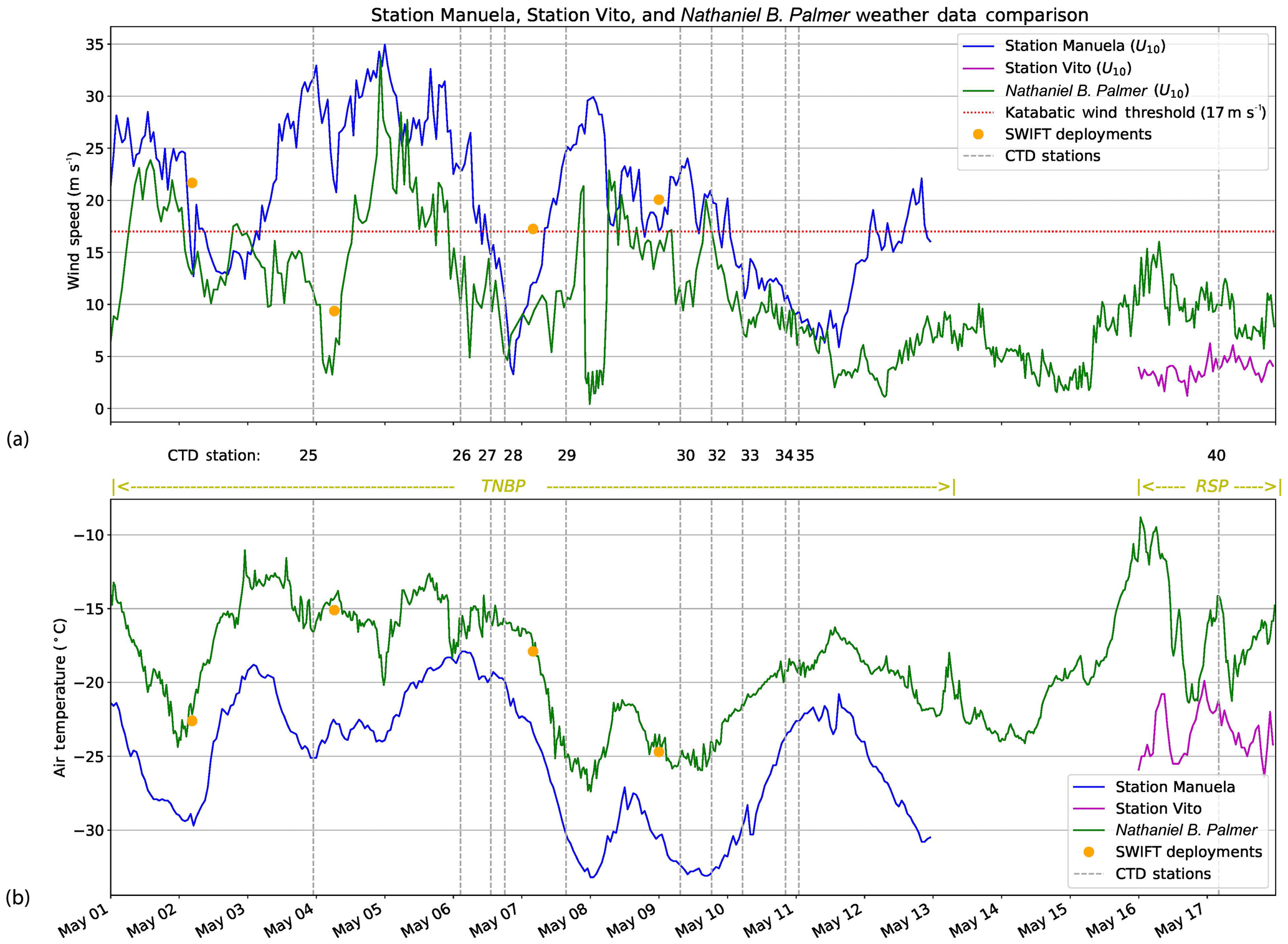
Figure 3 Weather observations from 1 to 17 May 2017. (a) Wind speed from Station Manuela (blue line), Station Vito (purple line), RVIB Nathaniel B. Palmer (green line), and SWIFT (orange marker) deployments adjusted to 10 m. The commonly used katabatic threshold of 17 m s⁻¹ is depicted as a “dotted red line”, as well as the date and start time of each CTD cast. (b) Air temperature from Station Manuela, Station Vito, RVIB Nathaniel B. Palmer, and SWIFT deployments.

3 Evidence of frazil ice formation

3.1 Selection of profiles

We used the following selection criteria to identify profiles from the two polynyas that appeared to show frazil ice formation: (1) a deep mixed layer extending several hundred meters (Fig. S1), (2) in situ temperature readings below the freezing point in the near-surface water (upper 5 m), and (3) an anomalous bolus of warm and/or salty water within the top 20 m of the profile (Figs. 4 and 5). For context, all temperature profiles acquired during PIPERS (with the exception of one profile acquired well north of the Ross Sea continental shelf area at 60^∘ S, 170^∘ E) were plotted to show how polynya profiles compared to those outside of polynyas (Fig. S2).

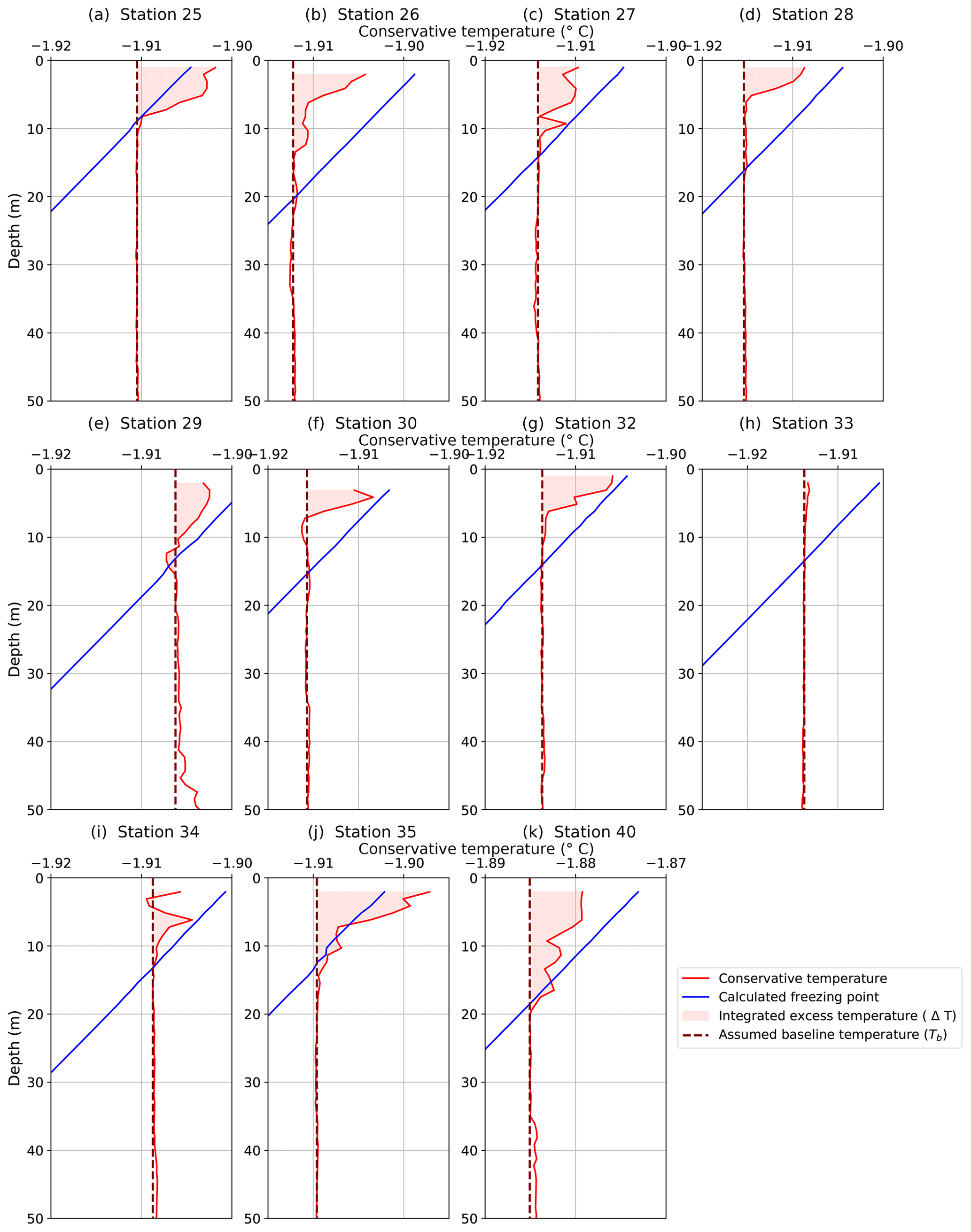
Figure 4 Conservative temperature profiles from CTD downcasts from 11 stations showing temperature and/or salinity anomalies. Plots (a–g, i–k) all show an anomalous temperature bulge. They also show supercooled water at the surface with the exceptions of (a, j). All of the plots have an x axis representing a 0.02 ^∘C change. Profiles (a–j) are from TNBP, and (k) is from RSP.

Polynya temperature profiles were then evaluated over the top 50 m of the water column using criteria 2 and 3. Nine TNBP profiles and one RSP profile exhibited excess temperature anomalies over the top 10–20 m and near-surface temperatures close to the freezing point (Fig. 4). Excess salinity anomalies (Fig. 5) were observed at the same stations with two exceptions: Station 26 had a measurable temperature anomaly (Fig. 4b) but no discernible salinity anomaly (Fig. 5b), and Station 33 had a measurable salinity anomaly (Fig. 5h) but no discernible temperature anomaly (Fig. 4h). The stations of interest are listed in Table 1.

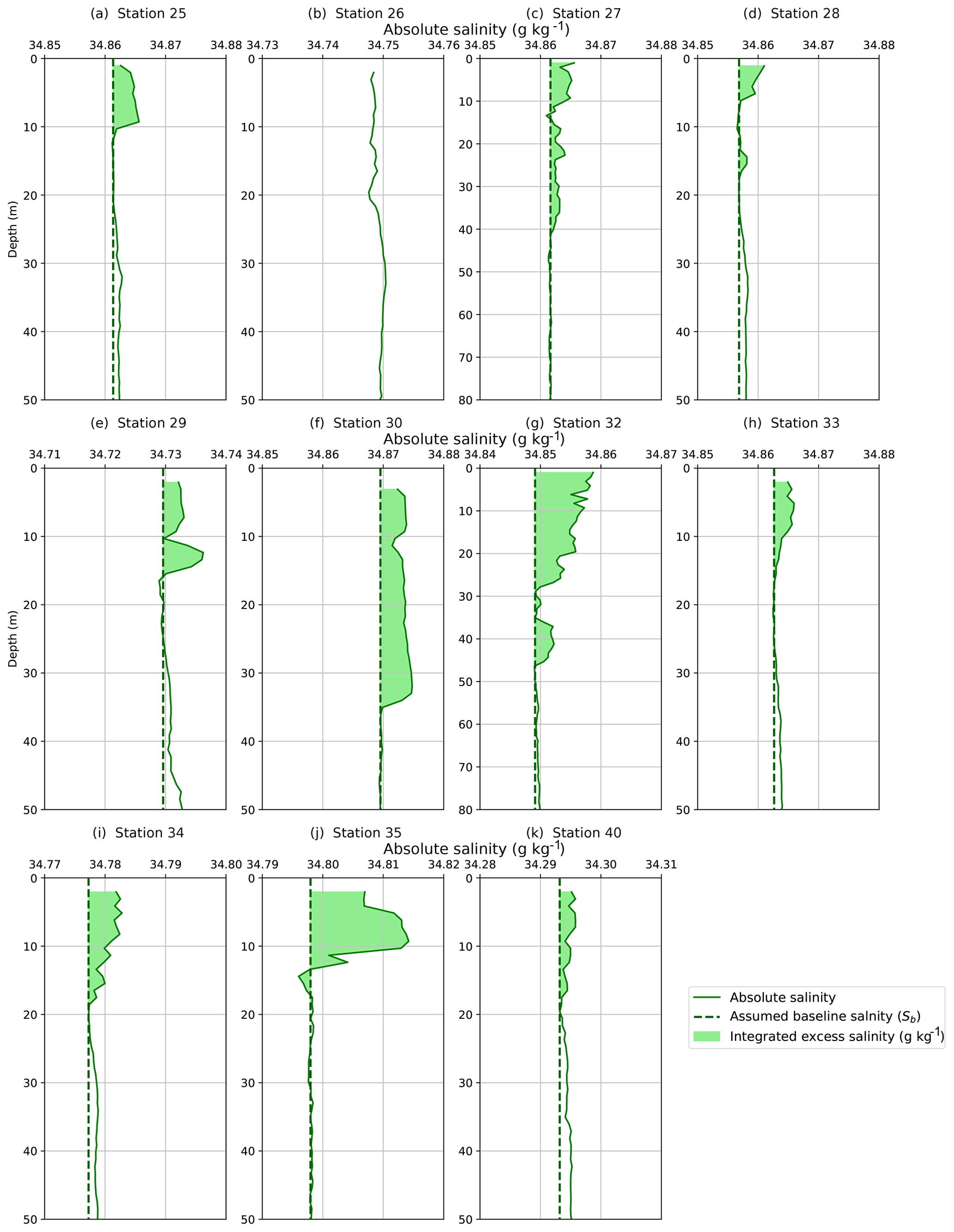
Figure 5 Absolute salinity profiles from CTD downcasts from 11 stations showing temperature and/or salinity anomalies. Profiles (a, c–k) show an anomalous salinity bulge in the top 10–20 m. Two profiles (c, g) show salinity anomalies extending below 40 m, so the plot was extended down to 80 m to best highlight those. All of the plots (a–k) have an absolute salinity range of 0.03 g kg⁻¹.

3.2 Evaluating the uncertainty in the temperature and salinity anomalies

We compared the magnitude of each thermal and haline anomaly to the reported accuracy of the SBE 911 temperature and conductivity sensors: ±0.001 ^∘C and ±0.0003 S m⁻¹, or ±0.00170 g kg⁻¹ when converted to absolute salinity. To quantify the magnitude of the temperature anomaly, we computed a baseline excursion, $\mathrm{\Delta }T=T_{\mathrm{obs}}-T_{\mathrm{b}}$, throughout the anomaly where T_obs is the observed temperature at that depth, and T_b is the in situ baseline temperature, which is extrapolated from the far-field temperature within the well-mixed layer below the anomaly (see Fig. 4 for schematic). The largest baseline excursion from each of the 11 anomalous CTD profiles, averaged together, yields a value of ΔT=0.0064 ^∘C. While this is a small absolute change in temperature, it is still 32 times larger than the stated precision of the SBE 911 (0.0002 ^∘C). The same approach was applied to the salinity anomalies and yielded an average baseline excursion of 0.0041 S m⁻¹ (or 0.0058 g kg⁻¹ for absolute salinity), which is 100 times larger than the instrument precision (0.00004 S m⁻¹). Table 1 lists the maximum temperature and salinity anomalies for each CTD station.

The immersion of instruments into supercooled water can lead to a number of unintended outcomes as instrument surfaces may provide ice nucleation sites or otherwise perturb an unstable equilibrium. Robinson et al. (2020) highlight a number of the potential pitfalls. One concern was that ingested frazil ice crystals could interfere with the conductivity sensor. Crystals smaller than 5 mm can enter the conductivity cell, creating spikes in the raw conductance data. Additionally, frazil crystals smaller than 100 µm would be small enough to pass between the conductivity electrodes and decrease the resistance/conductance that is reported by the instrument (Skogseth et al., 2009; Robinson et al., 2020). To test for ice crystal interference, the raw (unfiltered with no bin averaging) salinity profile was plotted and compared with the 1 m binned data for the 11 anomalous CTD stations (Fig. S3). The raw data showed varying levels of noise as well as some spikes or excursions to lower levels of conductance; these spikes may have been due to ice crystal interference. Overall, the bin-averaged profile does not appear to be biased or otherwise influenced by the spikes, which tend to fall symmetrically around a baseline. This was demonstrated by bin averaging over different depth intervals as described in Sect. 2.4. It is also worth pointing out that the effect of these conductivity spikes would be to decrease the bin-averaged salinity, thereby working against the overall observation of a positive baseline excursion. In other words, the entrainment of frazil crystals could lead to an underestimate of the positive salinity anomaly, rather than the production of positive salinity aberration.

Another pitfall highlighted by Robinson et al. (2020) is the potential for self-heating of the thermistor by residual heat in the instrument housing. The results from that study reveal a thermal inertia that dissipates over a period of minutes. We examined the temperature trace during the CTD soak and did not observe the same behavior. It is likely that some thermal inertia did exist at the time of deployment, but any residual heat appeared to dissipate very quickly, compared to the 3–6 min soak time before each profile. We suggest the self-heating might be a problem that arose in a single instrument but is not necessarily diagnostic of all SBE 911 instruments. Robinson et al. (2020) did not document this behavior in multiple instruments. Lastly, the potential for ice formation on the surface of the conductivity cell seems unlikely because it was kept warm until it was deployed in the water.

The observation of both warm and salty anomalies cannot easily be explained by these documented instrument biases. A cold instrument might experience freezing inside the conductivity cell, but this freezing would not influence the thermistor, which is physically separated from the conductivity cell. A warm instrument might have contained residual thermal inertia, which could melt individual frazil ice crystals, but these would produce negative baseline excursions in salinity, rather than a positive anomaly. The positive anomalies in temperature and salinity are not easily explained by these instrumental effects.

3.3 Camera observations of frazil ice formation

During PIPERS an EISCam (Evaluative Imagery Support Camera, version 2) was operating in time lapse mode, recording photos of the ocean surface from the bridge of the ship every 10 min (for more information on the EISCam see Weissling et al., 2009). The images from the time in TNBP and RSP reveal long streaks and large aggregations of frazil ice. A selection of photos from TNBP were captured (Fig. 6). The winds were strong enough at all times to advect frazil ice, creating downstream frazil streaks and eventually pancake ice in most situations. Smaller frazil streaks and a curtain of frazil ice below the frazil streak were also visible.

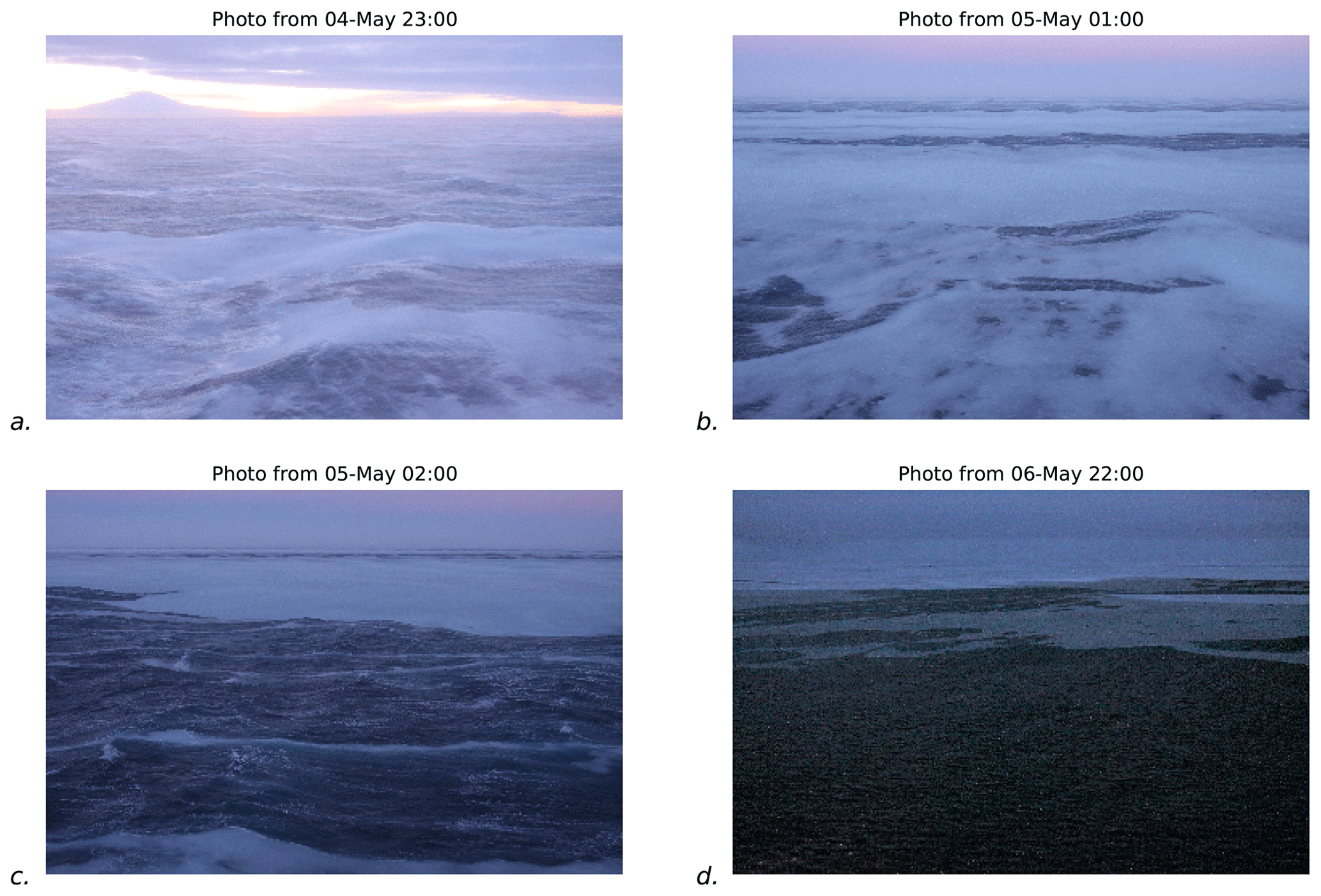
Figure 6 Images from RVIB Nathaniel B. Palmer as EISCam (Evaluative Imagery Support Camera) version 2. White areas in the water are loosely consolidated frazil ice crystals being actively formed during a katabatic wind event. Image (d) was brightened to allow for better contrast.

3.4 Conditions for frazil ice formation

Laboratory experiments can provide a descriptive picture of the conditions that lead to frazil ice formation; these conditions are diagnostic of conditions in the TNBP. Ushio and Wakatsuchi (1993) exposed a 2 m × 0.4 m × 0.6 m tank to air temperatures of −10 ^∘C and wind speeds of 6 m s⁻¹. They observed 0.1 to 0.2 ^∘C of supercooling at the water surface and found that after 20 min the rate of supercooling slowed due to the release of latent heat, coinciding with visual observation of frazil ice formation. After 10 min of ice formation, they observed a measurable increase in temperature of the frazil ice layer of 0.07 ^∘C warmer and 0.5 to 1.0 g kg⁻¹ saltier, as a consequence of latent heat and salt release during freezing (Ushio and Wakatsuchi, 1993).

In this study, we found the frazil ice layer to be on average 0.006 ^∘C warmer than the underlying water. Similarly, the salinity anomaly was on average 0.006 g kg⁻¹ saltier than the water below. While the anomalies we observed are smaller than those observed in the lab tank by Ushio and Wakatsuchi (1993), the trend of supercooling, followed by frazil ice formation and the appearance of a salinity anomaly, is analogous. The difference in magnitude can likely be explained by the reservoir size; the small volume of the lab tank will retain the salinity and temperature anomaly, rather than mixing it to deeper depths.

Considering the aggregate of supporting information, we infer that the anomalous profiles from TNBP and RSP were produced by frazil ice formation. The strong winds and subzero air temperatures (Sect. 2.4) reveal that conditions were sufficient for frazil formation, similar to the conditions observed in the laboratory. We showed that the CTD profiles in both temperature and salinity are reproducible and large enough to be distinguished from the instrument uncertainty (Sect. 3.1 and 3.2). Finally, the EISCam imagery reveals the accumulation of frazil ice crystals at the ocean surface.

4 Estimation of frazil ice concentration using CTD profiles

Having identified CTD profiles that trace frazil ice formation, we want to know how much frazil ice can be inferred from these T and S profiles. The inventories of heat and salt from each profile can provide independent estimates of frazil ice concentration. To simplify the inventory computations, we neglect the horizontal advection of heat and salt; this is akin to assuming that lateral variations are not important because the neighboring water parcels are also experiencing the same intense vertical gradients in heat and salt. We first describe the computation using temperature in Sect. 4.1 and the computation using salinity in Sect. 4.2.

4.1 Estimation of frazil ice concentration using temperature anomalies

Using the latent heat of fusion as a proxy for frazil ice production, we estimated the amount of frazil ice that must be formed in order to create the observed temperature anomalies. We estimated the excess enthalpy using the same temperature baseline excursion: $\mathrm{\Delta }T=T_{\mathrm{obs}}-T_{\mathrm{b}}$, defined in Sect. 3.2 . The excess over the baseline is graphically represented in Fig. 7a. Lacking multiple profiles at the same location, we are not able to observe the time evolution of these anomalies, so T_b represents the best inference of the temperature of the water column prior to the onset of ice formation; it is highlighted in Fig. 7a with the dashed line. The value of T_b was determined by averaging the profile temperature over a 10 m interval directly beneath the anomaly. In most cases, this interval was nearly isothermal and isohaline, as would be expected within a well-mixed layer. The uncertainty in the value of T_b was estimated from the standard deviation within this 10 m interval; the average was $\mathrm{7.5}\times {\mathrm{10}}^{-\mathrm{5}}$ ^∘C.

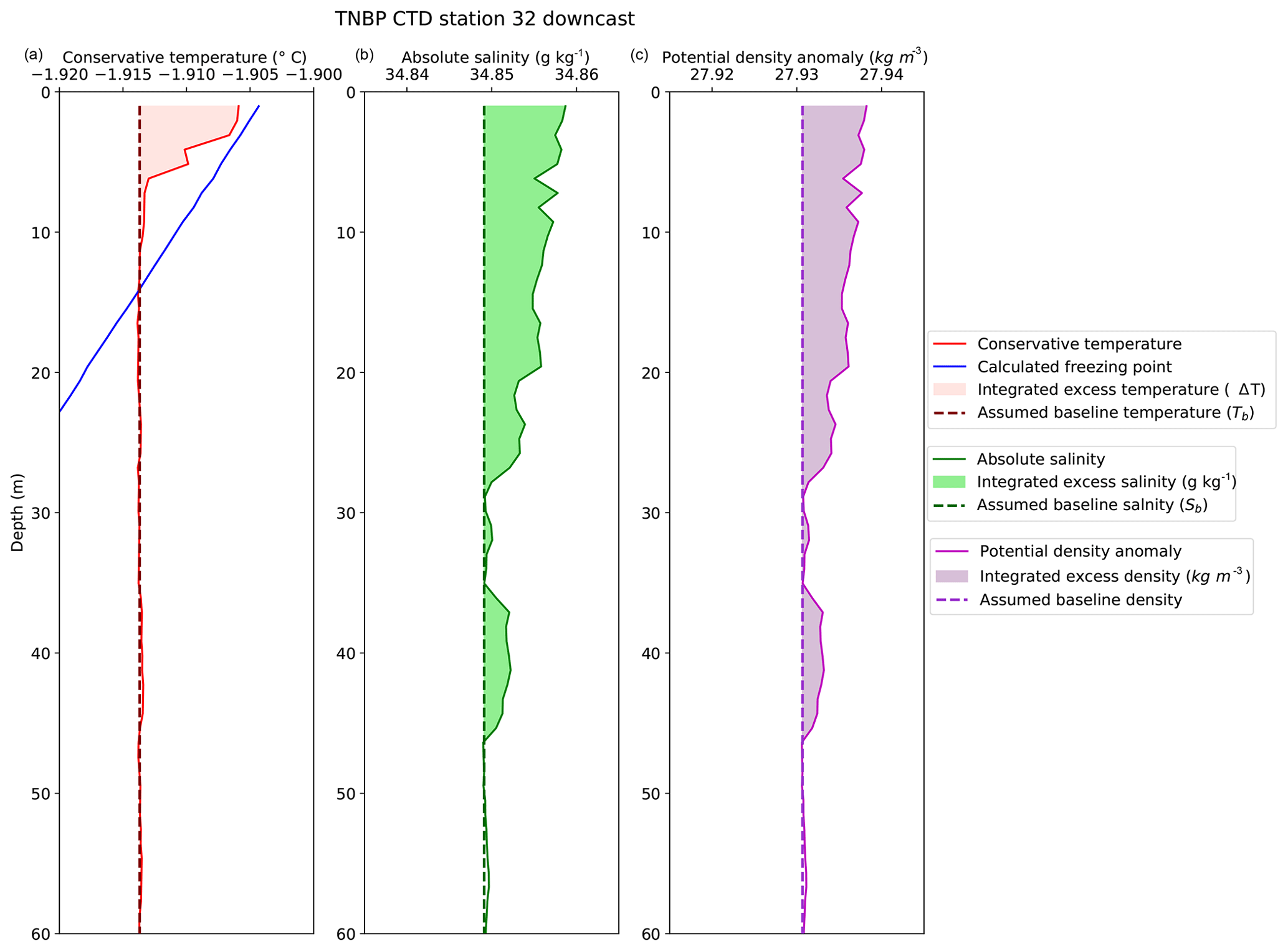
Figure 7 Conservative temperature, absolute salinity, and potential density anomaly for TNBP CTD Station 32, 9 May 2017. (a) Conservative temperature profile showing the temperature anomaly, the selected baseline temperature (dashed line), and the integrated excess temperature (shaded area). (b) Absolute salinity profile showing the salinity anomaly, the selected baseline salinity (dashed line), and integrated excess salinity (shaded area). (c) Potential density anomaly showing the selected baseline density (dashed) and the excess density instability (shaded).

To find the excess heat ($Q_{\mathrm{excess}}^{\mathrm{total}}$) contained within the thermal anomaly, we computed the vertical integral of heat per unit area from the surface (z=0) to the bottom of the anomaly (z=z_T):

$$\begin{array}{}\text{(1)}& Q_{\mathrm{excess}}^{\mathrm{total}}={\int }_{z=\mathrm{0}}^{z=z_T}\mathit{\rho }{C}_p^{\mathrm{W}}\mathrm{\Delta }T\mathrm{d}z.\end{array}$$

Here ρ is density of seawater, z is the depth range of the anomaly, and $C_p^{\mathrm{W}}$ is the specific heat capacity ($C_p^{\mathrm{W}}=\mathrm{3988}$ J kg⁻¹ K⁻¹ for TNBP; $C_p^{\mathrm{W}}=\mathrm{3991}$ J kg⁻¹ K⁻¹ for RSP). The concentration of frazil ice is estimated by applying the latent heat of formation (L_f=330 kJ kg⁻¹) as a conversion factor to $Q_{\mathrm{excess}}^{\mathrm{total}}$:

$$\begin{array}{}\text{(2)}& C_{\mathrm{ice}}^T={\displaystyle \frac{Q_{\mathrm{excess}}^{\mathrm{total}}}{L_{\mathrm{f}}{z}_T}}.\end{array}$$

The result from Eq. (2) represents the water column inventory of ice, in kilograms per cubic meter. A more detailed explanation of Eqs. (1) and (2) is contained in Sect. S1 in the Supplement and is itemized in Table 1.

4.2 Estimation of frazil ice concentration using salinity anomalies

The mass of salt within the salinity anomaly was also used to estimate ice formation. Assuming that frazil ice crystals do not retain any brine and assuming there is negligible evaporation, the salinity anomaly is directly proportional to the ice formed. By using the conservation equations for water and salt, the mass of frazil ice can be estimated by comparing the excess salt (measured as salinity) with the amount of salt initially present in the profile, similar to the inventory for heat. The complete derivation can be found in Sect. S2. The salinity anomaly (ΔS) above the baseline salinity (S_b) is $\mathrm{\Delta }S=S_{\mathrm{obs}}-S_{\mathrm{b}}$ and is shown in Fig. 7b. The initial value of salinity (S_b) was established by observing the trend in the salinity profile directly below the haline bulge. In most cases the salinity trend was nearly linear beneath the bulge; however in general the salinity profiles were less homogeneous than the temperature profiles. As with temperature, we determined S_b by averaging over a 10 m interval, starting below the anomaly. The uncertainty in the value of S_b was estimated from the standard deviation within this 10 m interval; the average was $\mathrm{2.8}\times {\mathrm{10}}^{-\mathrm{4}}$. To find the total mass of frazil ice per unit area ($M_{\mathrm{ice}}^S$, kg m⁻²) in the water column, the integral is taken as the salt ratio times the mass of water ($M_{\mathrm{W}}^O={\mathit{\rho }}_{\mathrm{b}}\mathrm{d}z$, where ρ_b is the assumed baseline density, or 1028 kg m⁻³). The concentration of ice ($C_{\mathrm{ice}}^S$, kg m⁻³) is found by dividing the mass of frazil ice by the depth of the salinity anomaly (z_s). The resulting estimates of ice concentration are listed in Table 1.

$$\begin{array}{}\text{(3)}& {\displaystyle }& {\displaystyle }{M}_{\mathrm{ice}}^S={\mathit{\rho }}_{\mathrm{b}}{\int }_{z=\mathrm{0}}^{z=z_S}{\displaystyle \frac{\mathrm{\Delta }S}{S_{\mathrm{obs}}}}\mathrm{d}z\text{(4)}& {\displaystyle }& {\displaystyle }{C}_{\mathrm{ice}}^S={\displaystyle \frac{M_{\mathrm{ice}}^S}{z_S}}\end{array}$$

A more detailed explanation of Eqs. (3) and (4) is contained in Sects. S2 and S3.

4.3 Summary of the frazil ice estimates

The salt inventories yielded frazil ice concentrations from $\mathrm{13}\times {\mathrm{10}}^{-\mathrm{3}}$ to $\mathrm{266}\times {\mathrm{10}}^{-\mathrm{3}}$ kg m⁻³, whereas the inventories based on heat range from 8 to $\mathrm{25}\times {\mathrm{10}}^{-\mathrm{3}}$ kg m⁻³ (Table 1). Within every profile the frazil ice concentration from the salinity inventory exceeds the concentration derived from the heat inventories, suggesting there is a systematic difference between the two. This difference can most likely be explained by loss of heat from the anomaly to the atmosphere. The same ocean heat loss that drives frazil ice production can also diminish the latent heat anomaly as it is produced. There is no corresponding loss term for the salt inventory. By the same token, it is worth noting that seawater evaporation may yield a small gain to the salt inventory. However, water vapor pressure is relatively small at these low air temperatures, and evaporative heat loss is a small term. Mathiot et al. (2012) found that evaporation had a small effect on salinity increases, when compared to ice production. In the TNBP, the Palmer meteorological tower revealed high relative humidity (on average 78.3 %), which indicates that there is likely some evaporation that would reduce the mass of ice derived from the salinity anomaly by a small (<4 %) margin (Mathiot et al., 2012). Taken together, these results suggest that the ice concentrations derived from the heat anomalies underestimate frazil ice concentration in comparison to the salt inventory; the salt inventory may overestimate the ice production, but the evaporation effect is minimal. For the remainder of the paper, we use the ice production estimates from the salt inventory and neglect the temperature inventory.

Table 1 CTD stations with temperature and salinity anomalies (see Figs. 4–5), showing maximum values of the temperature anomaly, depth range of the temperature anomaly, concentration of ice derived from the temperature anomaly (Sect. 4.1), and the maximum value of the salinity anomaly, depth range of salinity anomaly, and concentration of ice derived from the salinity anomaly (Sect. 4.2).

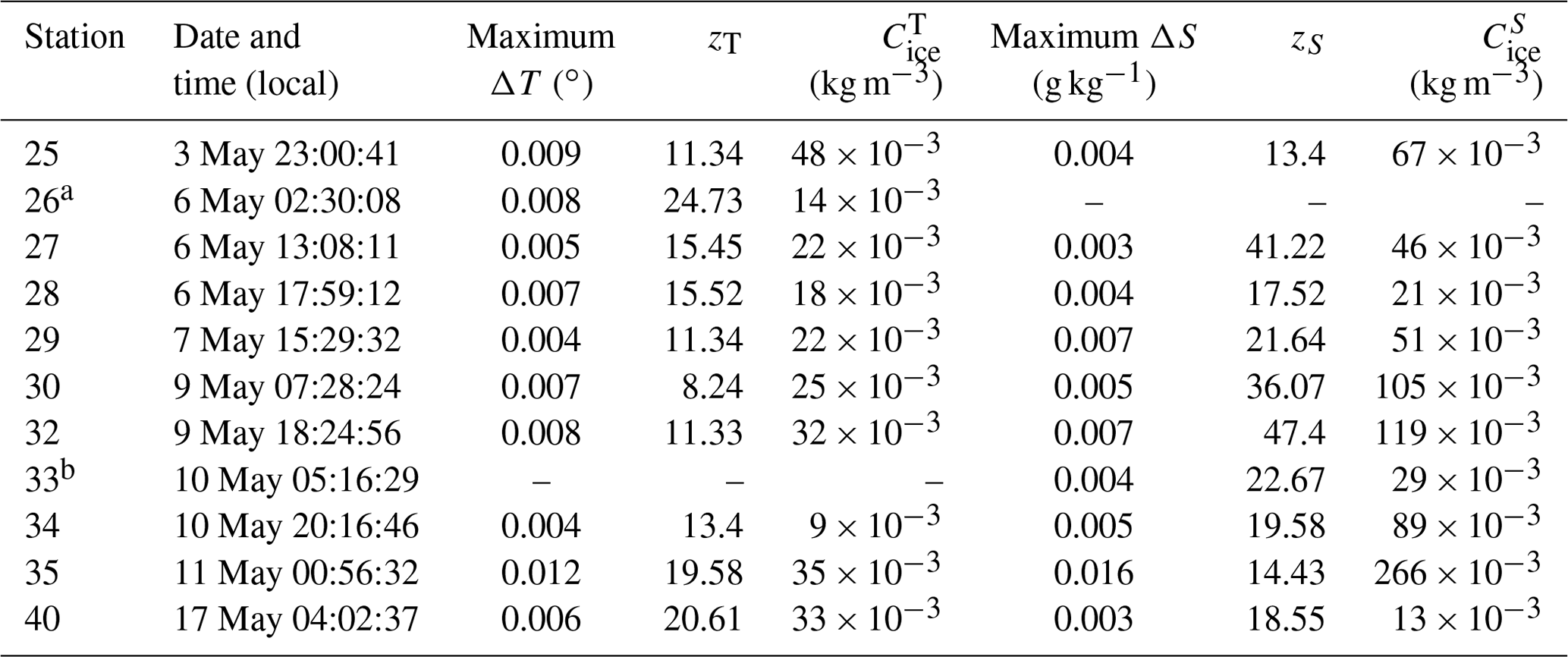
^a Station 26 did not have a measurable salinity anomaly but was included due to the clarity of the temperature anomaly. Conversely, ^b Station 33 did not have a measurable temperature anomaly but was included due to the clarity of the salinity anomaly.

5 Estimation of timescale of ice production

To better understand the characteristics of frazil ice production and the resulting water column signature, we can seek the lifetime of these T and S anomalies. Are they short-lived in the absence of forcing, or do they represent an accumulation over some longer ice formation period? One possibility is that the anomalies begin to form at the onset of the katabatic wind event, implying that the time required to accumulate the observed heat and salt anomalies is similar to that of a katabatic wind event (e.g., 12–48 h). This, in turn, would suggest that the estimates of frazil ice concentration have accumulated over the lifetime of the katabatic wind event. Another interpretation is that the observed anomalies reflect the near-instantaneous production of frazil ice. In this scenario, heat and salt are simultaneously produced and actively mixed away into the far field. In this case, the observed temperature and salinity anomalies reflect the net difference between production and mixing. One way to frame the question of the anomaly lifetime is to ask “if ice production stopped, how long would it take for the heat and salt anomalies to dissipate?” The answer depends on how vigorously the water column is mixing. In this section, we examine the mixing rate. However, we can first get some indication of the timescale by the density profiles.

5.1 Apparent instabilities in the density profiles

The computed density profiles reveal an unstable water column for all but one of our 11 stations (Fig. 8). These suggest that buoyancy production from excess heat did not effectively offset the buoyancy loss from excess salt within each anomaly. It is not common to directly observe water column instability without the aid of microstructure or other instruments designed for measuring turbulence.

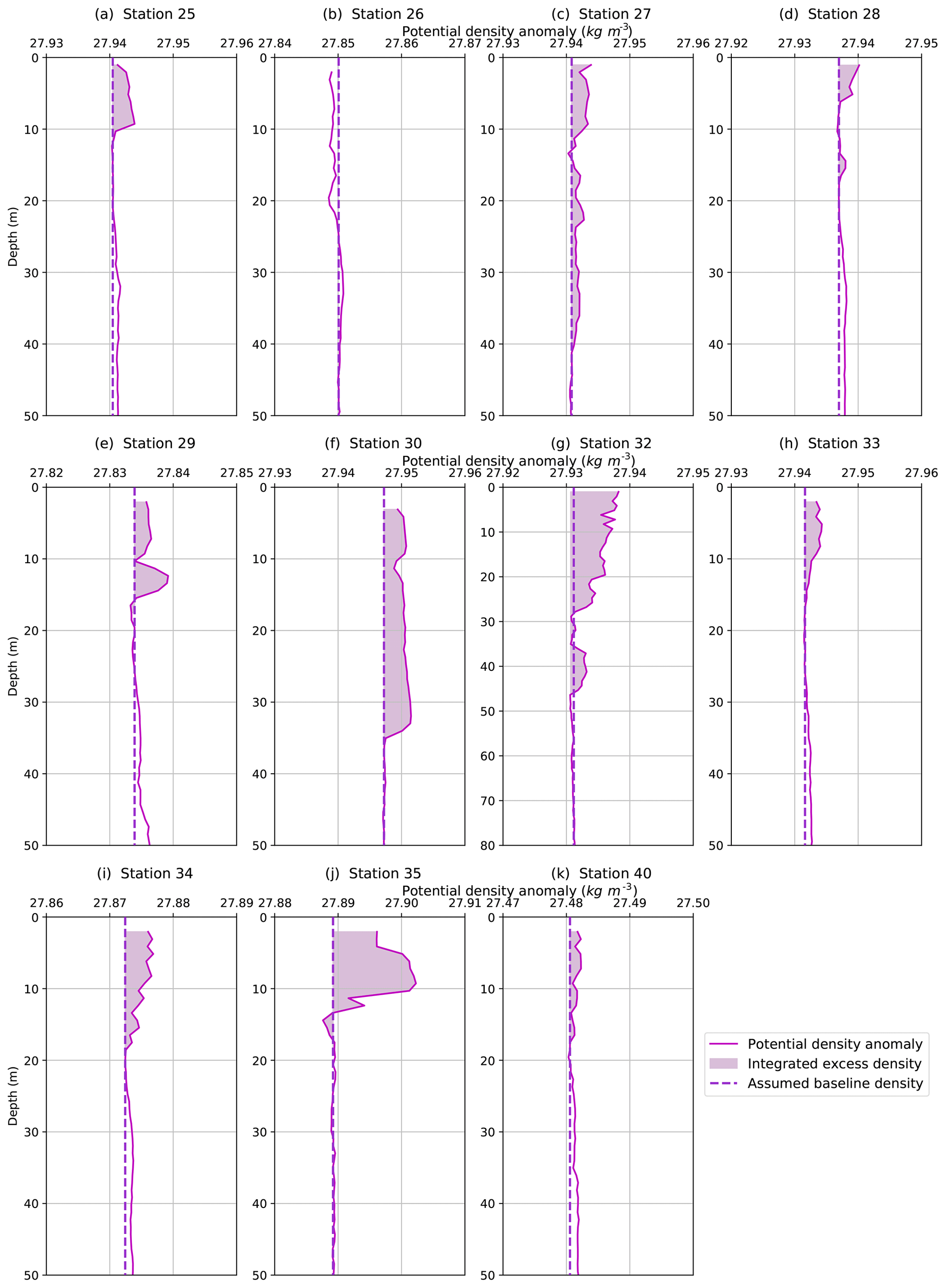
Figure 8 Potential density anomalies for all 11 stations with evidence of active frazil ice formation. The integrated excess density and assumed baseline density are depicted to highlight the instability. Note that Station 26 (b) does not present a density anomaly because it does not have a salinity anomaly. In the absence of excess salinity, the temperature anomaly instead created an area of less dense water (i.e., a stable anomaly).

An instability in the water column that persists long enough to be measured in a CTD profile must be the result of a continuous buoyancy loss that is created at a rate faster than it can be eroded by mixing. In other words, the katabatic winds appeared to dynamically maintain these unstable profiles. Continuous ice production leads to the production of observed heat and salt excesses at a rate that exceeds the mixing rate. If the unstable profiles reflect a process of continuous ice production, then the inventory of ice that we infer from our simple heat and salt budgets must reflect ice production during a relatively short period of time, defined by the time it would take to mix the anomalies away, once the wind-driven dynamics and ice production stopped.

Robinson et al. (2014) found that brine rejection from platelet ice formation also leads to dense water formation and a static instability. Frazil ice can form in ice shelf water that is subjected to adiabatic cooling during its buoyant ascent from beneath the ice shelf. This leads to a supercooled water mass, ice nucleation, and stationary instability, which was observable before being mixed away by convection (Robinson et al., 2014). This process does not take place at 200–300 m water depth, away from the air–sea interface, but it results in a water column signature that is similar to those observed in this study.

5.2 Lifetime of the salinity anomalies

To estimate the lifetime of each salinity anomaly requires an estimate of the rate of turbulent mixing in the mixed layer. The Kolmogorov theory for turbulent energy distribution defines the eddy turnover time as the time it takes for a parcel to move a certain distance, d, in a turbulent flow (Vallis, 2017). The smallest eddy scale is that of turbulent energy dissipation, and the largest scale is bounded by the length of the domain and the free-stream turbulent velocity (Cushman-Roisin, 2019). This timescale can be estimated as

$$\begin{array}{}\text{(5)}& t\approx {\displaystyle \frac{d}{{\left(\mathit{\epsilon }d\right)}^{\frac{\mathrm{1}}{\mathrm{3}}}}}\approx {\left({\displaystyle \frac{d^{\mathrm{2}}}{\mathit{\epsilon }}}\right)}^{\frac{\mathrm{1}}{\mathrm{3}}}.\end{array}$$

Here, d is the characteristic length of the largest eddy and ε is the turbulent kinetic energy (TKE) dissipation rate, which is related to the free-stream velocity as $\mathit{\epsilon }\sim w^{\mathrm{3}}/d$ (Cushman-Roisin, 2019). In this section we discuss and derive the best available estimates of t using measurements of the meteorological forcing conditions and in situ measurements of the turbulence.

If d is bounded only by the domain (in this case, the mixed-layer depth), this would suggest vertical turbulent eddies up to 600 m in length (Table 2). However, a homogenous mixed layer does not necessarily imply active mixing throughout the layer (Lombardo and Gregg, 1989). Instead, the length scale of the domain is more appropriately estimated from the size of the buoyancy instability and the background wind shear, or the Monin–Obukhov length (L_M−O) (Monin and Obukhov, 1954). When L_M−O is small and positive, buoyant forces are dominant and when L_M−O is large and positive, wind shear forces are dominant (Lombardo and Gregg, 1989). The L_M−O is estimated using the salt-driven buoyancy flux, reflecting the same process that gave rise to the observed salinity anomalies (see Sect. 4.3 for more detail).

$$\begin{array}{}\text{(6)}& L_{\mathrm{M}-\mathrm{O}}=-{\displaystyle \frac{u_{*}^{\mathrm{3}}}{k\mathit{\beta }gw\stackrel{\mathrm{‾}}{\mathrm{\Delta }S}}},\end{array}$$

where u_* is the aqueous friction velocity, g is gravitational acceleration, w is the water vertical velocity, $\stackrel{\mathrm{‾}}{\mathrm{\Delta }S}$ is the salt flux, β is the coefficient of haline contraction, and k is the von Kármán constant. A more detailed explanation and the specific values are listed in Sect. S4.

The friction velocity derives from the wind speed (U_P), measured at the RVIB Nathaniel B. Palmer weather mast from a height of z_P=24 m, adjusted to a 10 m reference (U₁₀) (Manwell et al., 2010).

$$\begin{array}{}\text{(7)}& U_{\mathrm{10}}=U_{\mathrm{P}}{\displaystyle \frac{\ln \left(\frac{z}{z_{\mathrm{o}}}\right)}{\ln \left(\frac{z_{\mathrm{P}}}{z_{\mathrm{o}}}\right)}}\end{array}$$

Roughness class 0 was used in the calculation and has a roughness length of 0.2 µm. These values are used to estimate the wind stress as

$$\begin{array}{}\text{(8)}& \mathit{\tau }=C_{\mathrm{D}}{\mathit{\rho }}_{\mathrm{air}}{U}_{\mathrm{10}}^{\mathrm{2}},\end{array}$$

where ρ_air represents the density of air, with a value of 1.3 kg m⁻³ calculated using averages from RVIB Nathaniel B. Palmer air temperature (−18.7 ^∘), air pressure (979.4 mbar), and relative humidity (78.3 %). C_D, the dimensionless drag coefficient, was calculated as $\mathrm{1.525}\times {\mathrm{10}}^{-\mathrm{3}}$ using the NOAA COARE 3 model, modified to incorporate wave height and speed (Fairall et al., 2003). The average weather data from RVIB Nathaniel B. Palmer was paired with the wave height and wave period from the SWIFT deployment (Surface Wave Instrument Float with Tracking) on 4 May to find C_D. A more detailed explanation and the specific values are listed in Sect. S5. Finally, u_* from Eq. (6) is

$$\begin{array}{}\text{(9)}& u_{*}=\sqrt{{\displaystyle \frac{\mathit{\tau }}{{\mathit{\rho }}_{\mathrm{water}}}}}.\end{array}$$

During the katabatic wind events, a SWIFT buoy was deployed to measure ε, w, and wave field properties (Thomson, 2012; Thomson et al., 2016; Zippel and Thomson, 2016). SWIFT deployments occurred within the period of CTD observations, as shown in the timeline of events (Fig. S5); however they do not coincide in time and space with the CTD profiles. For the vertical velocity estimation, we identified the 4 and 9 May SWIFT deployments as most coincident to CTD stations analyzed here, based on similarity in wind speeds. The average wind speed at all the CTD stations with anomalies was 10.2 m s⁻¹. For the 4 May SWIFT deployment, the wind speed was 9.36 m s⁻¹. CTD Station 32 experienced the most intense sustained winds of 18.9 m s⁻¹. The 9 May SWIFT deployment was applied to CTD 32, which had a wind speed of 20.05 m s⁻¹. During these SWIFT deployments, 4 May had an average value of w=0.015 m s⁻¹ and 9 May had an average value of w=0.025 m s⁻¹.

The TKE dissipation rates are expected to vary with wind speed, wave height, and ice thickness and concentration (Smith and Thomson, 2019). Wind stress is the source of momentum to the upper ocean, but this is modulated by scaling parameter (c_e, Smith and Thomson, 2019). If the input of TKE is in balance with the TKE dissipation rate over an active turbulent layer, the following expression can be applied:

$$\begin{array}{}\text{(10)}& c_{\mathrm{e}}\mathit{\tau }\propto \mathit{\rho }\int \mathit{\epsilon }\left(z\right)\mathrm{d}z,\end{array}$$

where the density of water (ρ) is assumed to be 1027 kg m⁻³ for all stations. This scaling parameter incorporates both wave and ice conditions; more ice produces more efficient wind energy transfer, while simultaneously damping surface waves, with the effective transfer velocity in ice. Smith and Thompson (2019) used the following empirical determination of c_e:

$$\begin{array}{}\text{(11)}& c_{\mathrm{e}}=a{\left(A{\displaystyle \frac{z_{\mathrm{ice}}}{H_{\mathrm{s}}}}\right)}^{\mathrm{b}}.\end{array}$$

Here, A is the fractional ice cover, with a maximum value of 1, z_ice is the thickness of ice, and H_s is the significant wave height. Using Antarctic Sea-ice Processes and Climate (ASPeCt) visual ice observations (http://www.aspect.aq, last access: 15 April 2020) from RVIB Nathaniel B. Palmer, the fractional ice cover and thickness of ice were found at the hour closest to both SWIFT deployments and CTD profiles (Knuth and Ackley, 2006; Ozsoy-Cicek et al., 2009; Worby et al., 2008). SWIFT wave height measurements yielded an average value of H_s=0.58 m for 4 May, and this value was applied to all the CTD profiles. To obtain the most robust data set possible, in total, 13 vertical SWIFT profiles from 2, 4, and 9 May were used to evaluate Eq. (12) over an active depth range of 0.62 m.

Using the estimates of c_e, τ, and ε from SWIFT, we parameterized the relationship between wind stress and ε that is reflected in Eq. (10). A linear fit on a log–log scale ($y={\mathrm{10}}^{\left(\mathrm{1.4572}\log \mathrm{10}\right(x)+\mathrm{0.2299})}$, r²=0.6554) was then applied to RVIB Nathaniel B. Palmer wind stress data to derive estimates of ε that coincided with the ambient wind conditions at each CTD station (Table 2).

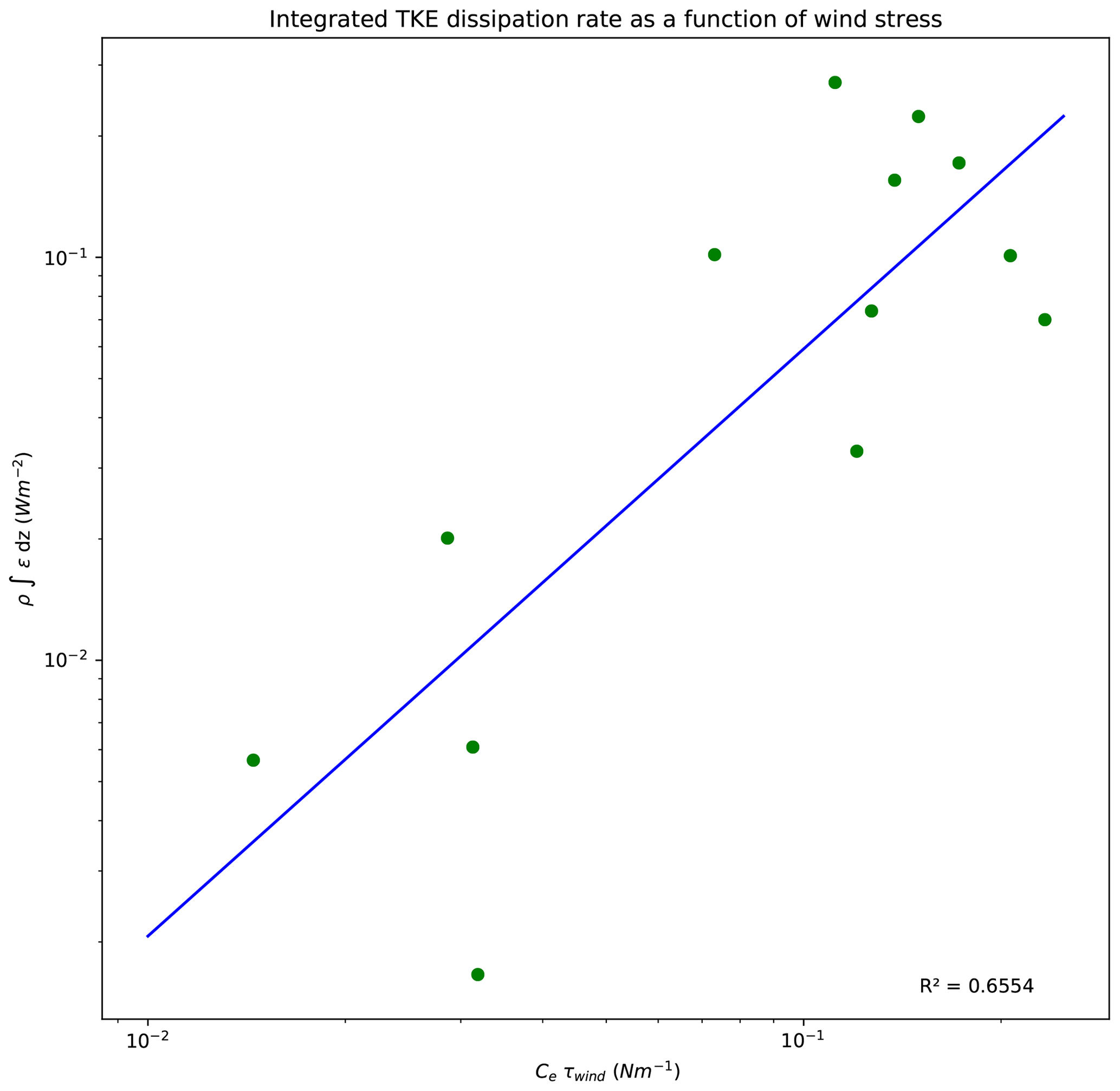
Figure 9 Vertical integral of ε, the TKE dissipation rate, estimated from the SWIFT buoy deployments, versus estimates of wind-driven TKE inputs into the surface ocean. A linear scaling relationship was applied to the log of each property.

Gathering these estimates of w, u_*, and ε, we estimate the anomaly lifetime using Eq. (5). Because L_M−O represents the domain length scale, we rewrite Eq. (5) as

$$\begin{array}{}\text{(12)}& t={\left({\displaystyle \frac{L_{\mathrm{M}-\mathrm{O}}^{\mathrm{2}}}{\mathit{\epsilon }}}\right)}^{\frac{\mathrm{1}}{\mathrm{3}}}.\end{array}$$

The values used to estimate L_M−O were computed as follows: haline contraction, β, in Eq. (6) was calculated from the Gibbs SeaWater toolbox and averaged over the depth range of the anomaly. The excess salt, $\stackrel{\mathrm{‾}}{\mathrm{\Delta }S}$, was found using the average value of ΔS for each profile anomaly. The values of L_M−O range from 6 to 330 m (Table 2). In general, L_M−Owas greater than the length of the salinity anomaly but smaller than the mixed-layer depth.

The mixing lifetime of these salinity anomalies ranged from 2 to 12 min, but most values cluster near the average of 9 min. The average timescale is similar to the frazil ice lifetime found in Michel (1967). These lifetimes suggest that frazil ice production and the observed density instabilities would relax to a neutral profile within 10 min of a diminution in wind forcing.

6 Rate of frazil ice production

We can extend the analysis of anomaly lifetime to estimate the frazil ice production rate. Heuristically, if turbulence production and dissipation are in balance, the lifetime of the anomaly is equivalent to the time it would take for the anomaly to be dissipated, or produced, given the observed conditions of heat loss to the atmosphere. By that analogy, the sea ice production rate is

$$\begin{array}{}\text{(13)}& r_{\mathrm{ice}}={\displaystyle \frac{C_{\mathrm{ice}}^S{z}_S}{t{\mathit{\rho }}_{\mathrm{ice}}}}.\end{array}$$

Here, ρ_ice=920 kg m⁻³; as previously defined, z_s is the depth of the salinity anomaly in meters. The results are summarized in Table 2 (see Sect. S6 for additional detail). To bound the uncertainty in r_ice, we estimated the 95 % confidence interval (CI) for ε at each CTD station. These are expressed as the range of ice production rates in Table 2. Uncertainty in the heat and salt inventories were not included in the uncertainty estimates, because we observed negligible differences in the inventory while testing the inventory for effects associated with bin averaging of the CTD profiles (Sect. 2.3). Another small source of error arises from neglecting evaporation. To quantify uncertainties introduced by that assumption, we used the bulk aerodynamic formula for latent heat flux and found the effects of evaporation across the CTD stations to be 1.8 % [0.07 %–3.45 %] (Zhang, 1997). The uncertainty from the effects of evaporation are similar to those of Mathiot et al. (2012). On average, the lower limit of ice production was 30 % below the estimate, and the upper limit was some 44 % larger than the estimated production.

The estimates of frazil ice production rate span 2 orders of magnitude, from 3 to 302 cm d⁻¹, with a median ice production of 28 cm d⁻¹. The highest ice production estimate occurred at CTD 35, closest to the Antarctic coastline and the Nansen Ice Shelf. The next largest value is 110 cm d⁻¹, suggesting the ice production at CTD 35 is an outlier and may have been influenced by platelet ice in upwelling ice shelf water that originated beneath the Nansen Ice Shelf (Robinson et al., 2014). In case there is an ice shelf water influence recorded in CTD 35, it will be excluded from the remainder of this analysis.

The remaining ice production rates span a range from 3 to 110 cm d⁻¹ and reveal some spatial and temporal trends that correspond with the varying conditions in different sectors of the TNBP. A longitudinal gradient emerges along the length of the polynya, when observing a subset of stations, categorized by similar wind conditions CTD 30 (U₁₀=11.50 m s⁻¹), CTD 27 (U₁₀=10.68 m s⁻¹), and CTD 25 (U₁₀=11.77 m s⁻¹). Beginning upstream near the Nansen Ice Shelf (Station 30) and moving downstream along the predominant wind direction toward the northeast, the ice production rate decreases. The upstream production rate is 63 cm d⁻¹ followed by midstream values of 28 cm d⁻¹ and lastly downstream values of 14 cm d⁻¹.

The spatial trend we observed somewhat mimics the 3D model of TNBP from Gallee (1997). During a 4 d simulation, Gallee found the highest ice production rates near the coast of 50 cm d⁻¹, which decreased to 0 cm d⁻¹ downstream and at the outer boundaries, further west than PIPERS Station 33 (Fig. 10). Some of the individual ice production rates derived from PIPERS CTD profiles (e.g., 110 cm d⁻¹) appear quite large compared to previous estimates; however it is worth emphasizing the dramatically different timescale that applies to these estimates. These “snapshots”, which capture ice production on the scale of tens of minutes, are more likely to capture the high frequency variability in this ephemeral process. As the katabatic winds oscillate, the polynyas enter periods of slower ice production, driving average rates down. To produce a comparable estimate, we attempt to scale these results to a seasonal average in the next section.

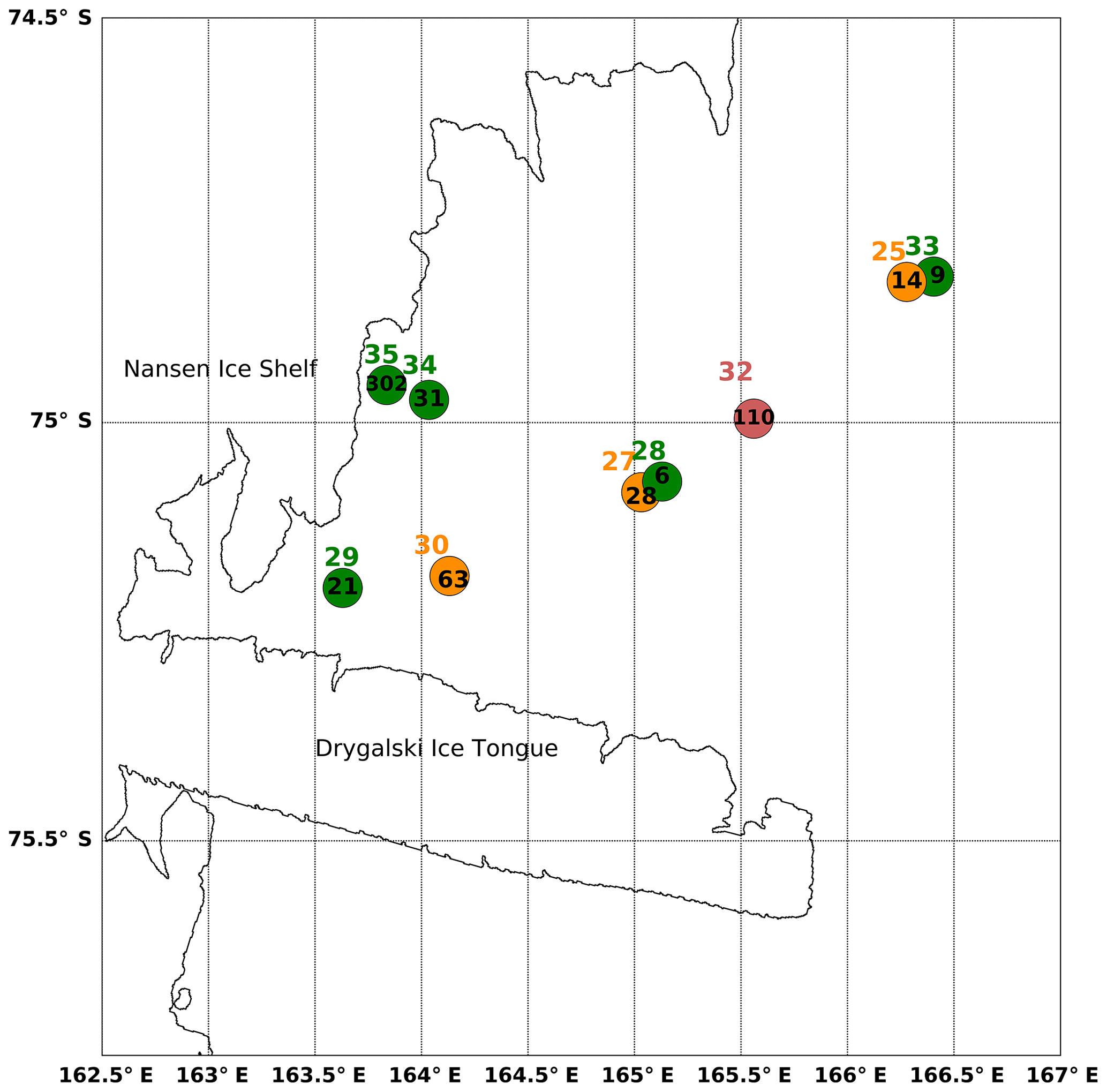
Figure 10 Map of TNBP CTD stations with anomalies and ice production rates. The CTD station number is listed to the north of the stations. The value inside the circle is the ice production rate (at that station) in centimeters per day. The symbols and station numbers are colored by wind speed: green indicates wind speeds less than 10 m s⁻¹ (Stations 28, 29, 33, 34, 35), orange indicates wind speeds between 10 and 15 m s⁻¹ (Stations 25, 27, 30), and red indicates wind speeds over 15 m s⁻¹ (Station 32).

Table 2 Summary of mass of ice derived from salinity, lifetime, and production rates.

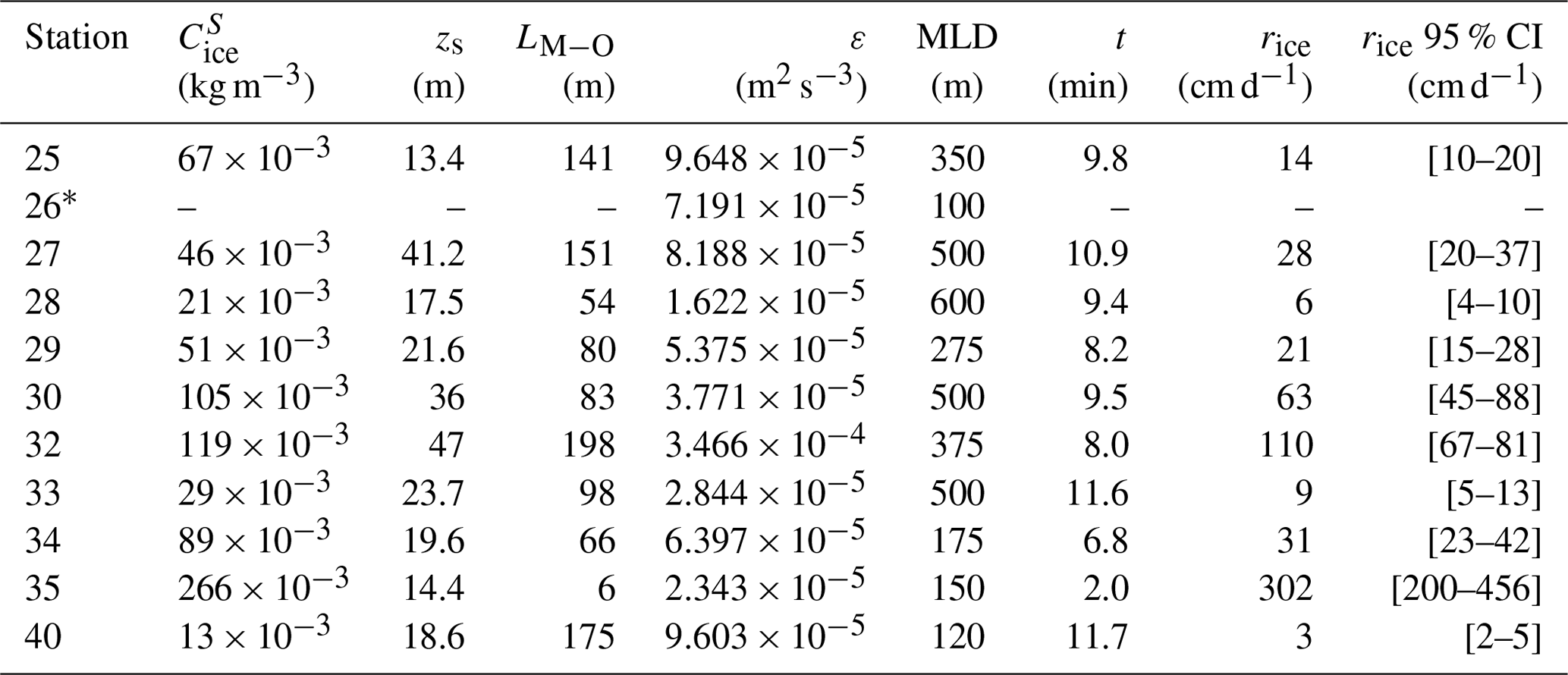
^* Station 26 did not have a measurable salinity anomaly but was included due to the clarity of the temperature anomaly. The term MLD stands for estimated mixed-layer depth.

6.1 Seasonal ice production

We estimate the seasonal average in sea ice production by relating these in situ ice production estimates to the time series atmospheric forcing from the automated weather stations, which extend over the season. The sensible heat flux (Q_s) is used as a diagnostic term to empirically scale the ice production rates for the season.

$$\begin{array}{}\text{(14)}& Q_{\mathrm{s}}=C_p^{\mathrm{A}}{\mathit{\rho }}_{\mathrm{a}}{C}_{\mathrm{s}}{u}_{\mathrm{10}}\left(T_{\mathrm{b}}-T_{\mathrm{a}}\right)\end{array}$$

Here $C_p^{\mathrm{A}}=\mathrm{1.003}$ kJ kg⁻¹ K⁻¹, the specific heat capacity of air at −23 ^∘C, and $C_{\mathrm{s}}=\mathrm{1.297}\times {\mathrm{10}}^{-\mathrm{3}}$, the heat transfer coefficient calculated using the COARE 3.0 code (Fairall et al., 2003). The values are included in Table S6 in the Supplement.

First, the sensible heat flux was calculated at each TNBP CTD station using the coincident RVIB Nathaniel B. Palmer meteorological data. Station 35 (see Sect. 5.1) and Station 40, in the Ross Sea polynya, were excluded from this calculation. Figure 11 depicts the trend between Q_s and sea ice production rate; the high degree of correlation (R²=0.915) likely occurs because the same RVIB Nathaniel B. Palmer wind speeds were used in the calculation of both Q_s and sea ice production (Eq. 7); in other words, the two terms are not strictly independent of each other.

Figure 11 Empirical relationship between sensible heat flux and sea ice production: production rate $=\mathrm{0.1785}{Q}_{\mathrm{s}}-\mathrm{28.048}$; R² is 0.915.

Next, the empirical trend was applied to a time series of Q_s from Station Manuela. The met data from the RVIB Nathaniel B. Palmer and from Station Manuela (Fig. 3) reveal that TNBP experiences slower wind speeds and warmer temperatures than Station Manuela. This phenomenon has been explained as a consequence of adiabatic warming and a reduction in the topographic “Bernoulli” effects that cause wind speed to increase at Station Manuela (Schick, 2018). Before applying the time series of met data from Manuela to Eq. (14) to calculate Q_s, we need to account for the offset. On average, the air temperatures were 6.5 ^∘C warmer, and wind speed was 7.5 m s⁻¹ slower in TNB, during the 13 d that the vessel was in the polynya. Figure S6 shows the corrected data against the original data for the time in TNB.

We estimated the seasonal average in Q_s over TNBP using the corrected met data from Station Manuela and an average sea surface temperature from the CTD stations (−1.91 ^∘C). The air density, specific heat capacity, and heat transfer coefficient remained the same as above.

The average inQ_s from April to September is 321 W m⁻². Using the empirical relationship described in Fig. 11, the seasonal average of frazil ice production in Terra Nova Bay polynya is 29 cm d⁻¹.

The seasonal sea ice production rate varies based on many factors affecting the rate of heat loss from the surface ocean. These factors include a strong negative feedback between ocean heat loss and sea ice cover. As the polynya builds up with ice, heat fluxes to the atmosphere will decline (Ackley et al., 2020) until that ice cover is swept out of the polynya by the next katabatic wind event. This spatial variation in ice cover and wind speed produces strong spatial gradients in the heat loss to the atmosphere that, in turn, drives ice production. For example, Ackley et al. (2020) observed heat flux variations from nearly 2000 W m⁻² to less than 100 W m⁻² over less than 1 km. An integrated estimate of total polynya sea ice production should take these spatial gradients and the changes in polynya area into account. That analysis is somewhat beyond the scope of this study, but we anticipate including these ice production estimates within forthcoming sea ice production estimates for 2017 and PIPERS.

One interesting outcome of the scaling relationship in Fig. 11 is the value of the y intercept at 157 W m⁻². This relationship suggests that frazil ice production ceases when the heat flux falls below this range. This lower bound, in combination with the spatial gradients in heat flux, may help to establish the region where active production is occurring.

6.2 Comparison to prior model and field estimates of ice production

The seasonal average ice production of 29 cm d⁻¹ estimated here falls within the upper range of other in situ ice production estimates. Schick (2018) estimated a seasonal average ice production rate of 15 cm d⁻¹, and Kurtz and Bromwich (1985) determined 30 cm d⁻¹. Both studies derived their ice production rates using a heat budget.

Overall, the ice production estimates from in situ data, including heat flux estimates, are larger than the seasonal ice production estimates derived from remote sensing products. Drucker et al. (2011) used the AMSR-E instrument to obtain a seasonal average of 12 cm d⁻¹ for the years 2003–2008. Ohshima et al. (2016) estimated 6 cm d⁻¹ of seasonal production for the years 2003–2011, and Nihashi and Ohshima (2015) determined 7 cm d⁻¹ for the years 2003–2010. Finally, Tamura et al. (2016) found production rates that ranged from 7 to 13 cm d⁻¹, using both ECMWF and NCEP Reanalysis products for 1992–2013, reflecting a greater degree of consistency in successive estimates, likely because of consistency in the estimation methods.

Using a sea ice model, Sansiviero et al. (2017) estimated seasonal average production of 27 cm d⁻¹, which falls closer to the estimates from in situ measurements. Petrelli et al. (2008) modeled an average daily rate of production of 14.8 cm d⁻¹ in the active polynya, using a coupled atmosphere–sea ice model. Fusco et al. (2002) applied a model for latent heat polynyas and estimated a seasonal average production rate of 34 cm d⁻¹ for 1993 and 29 cm d⁻¹ for 1994, which is comparable to the in situ budgets.

7 Conclusions

Polynyas have been regarded as ice production factories, which are responsible for total volumetric ice production that is vastly disproportionate to their surface area. This study documented temperature and salinity anomalies in the upper ocean that reflect vigorous frazil ice production in polynyas. These anomalies produce an unstable water column that can be observed as a quasi-stationary feature in the density profile. The only comparable example is found in the outflow of supercooled ice shelf waters, which occur much deeper in the water column. These features were observed during strong katabatic wind events in the Terra Nova Bay and the Ross Sea polynyas, with ocean heat losses to the atmosphere in excess of 2000 W m⁻². The anomalies provide additional insights into the ice production within polynyas and have provided estimates of frazil ice production rates, in situ. The frazil production rates vary from 3 to 110 cm d⁻¹, with a seasonal average of 29 cm d⁻¹, and the method captures ice production on the timescale of minutes to tens of minutes, which is significantly shorter than the more common daily or monthly production rates.

These estimates may suggest that frazil ice is a more significant ice type for ice production in polynyas than was previously thought. However, it is not clear how many frazil ice crystals survive to become part of the consolidated seasonal ice pack. In this vigorous mixing environment, a fraction may melt and become reincorporated into the ocean, before they have a chance to aggregate.

By the same token, frazil production and the estimates of ice production could be improved by collecting consecutive CTD casts at the same location to observe how these anomalies evolve on the minute-to-minute timescale, which can be challenging in regions of active ice formation. One exciting outcome of this study is the suggestion that it is possible to obtain synoptic inventories of ice production. For example, a float or glider that measures surface CTD profiles on a frequent basis would improve our synoptic and seasonal understanding of polynya ice production as they respond to annual and secular modes of the ocean and atmosphere.