Evaluating permafrost physics in the Coupled Model Intercomparison Project 6 (CMIP6) models and their sensitivity to climate change

Permafrost is a ubiquitous phenomenon in the Arctic. Its future evolution is likely to control changes in northern high-latitude hydrology and biogeochemistry. Here we evaluate the permafrost dynamics in the global models participating in the Coupled Model Intercomparison Project (present generation – CMIP6; previous generation – CMIP5) along with the sensitivity of permafrost to climate change. Whilst the northern high-latitude air temperatures are relatively well simulated by the climate models, they do introduce a bias into any subsequent model estimate of permafrost. Therefore evaluation metrics are defined in relation to the air temperature. This paper shows that the climate, snow and permafrost physics of the CMIP6 multi-model ensemble is very similar to that of the CMIP5 multi-model ensemble. The main differences are that a small number of models have demonstrably better snow insulation in CMIP6 than in CMIP5 and a small number have a deeper soil profile. These changes lead to a small overall improvement in the representation of the permafrost extent. There is little improvement in the simulation of maximum summer thaw depth between CMIP5 and CMIP6. We suggest that more models should include a better-resolved and deeper soil profile as a first step towards addressing this. We use the annual mean thawed volume of the top 2 m of the soil defined from the model soil profiles for the permafrost region to quantify changes in permafrost dynamics. The CMIP6 models project that the annual mean frozen volume in the top 2 m of the soil could decrease by 10 %–40 $\mathrm{\%}{}^{\circ }{\mathrm{C}}^{-\mathrm{1}}$ of global mean surface air temperature increase.

1 Introduction

Permafrost, defined as ground that remains at or below 0 ^∘C for 2 or more consecutive years, underlies 22 % of the land in the Northern Hemisphere (Obu et al., 2019). Permafrost temperatures increased by $\mathrm{0.29}\pm \mathrm{0.12}{}^{\circ }\mathrm{C}$ between 2007 and 2016 when averaged across polar and high-mountain regions (Pörtner et al., 2019; Biskaborn et al., 2019). This unprecedented change will have consequences for northern hydrological and biogeochemical cycles. For example, it will result in CO₂ and CH₄ emissions which will have a positive feedback on the global climate (Burke et al., 2017b). The ecology of thaw-impacted lakes and streams is also likely to change with microbiological communities adapting to changes in sediment, dissolved organic matter, and nutrient presence (Vonk et al., 2015). Conditions are likely to be more conducive to fire with earlier snowmelt and drier ground in spring (Wotton et al., 2017). Furthermore subsidence from thawing permafrost will cause damage to artificial infrastructures (Melvin et al., 2017; Hjort et al., 2018), leading to issues with the overall sustainability of northern communities (Larsen et al., 2014). The latest generation of the Coupled Model Intercomparison Project (CMIP6; Eyring et al., 2016) provides an opportunity to increase our understanding of these potential impacts under future climate change.

CMIP6 provides a coordinated set of earth system model simulations designed, in part, to understand how the earth system responds to forcing and to make projections for the future. Here we derive and apply a set of metrics to benchmark the ability of the coupled CMIP6 models to represent permafrost physical processes. Biases in the simulated permafrost arise from (1) biases in the simulated surface climate and (2) biases in the underlying land surface model. Where possible, this paper isolates the land surface component from the surface climate and focuses on the land surface component. Both Koven et al. (2013) and Slater et al. (2017) evaluated the previous generation of global climate models (CMIP5) and found that the spread of simulated present-day permafrost area within that ensemble is large and mainly caused by structural weaknesses in snow physics and soil hydrology within some of the models. Here we assess any improvements in the CMIP6 multi-model ensemble over the CMIP5 multi-model ensemble. Koven et al. (2013) and Slater and Lawrence (2013) also found a wide variety of permafrost states projected by the CMIP5 multi-model ensemble in 2100. We evaluate whether the sensitivity of permafrost to climate change is different in this current generation of CMIP models.

Permafrost dynamics can be described by the mean annual ground temperature at the top of the permafrost (MAGT) and the maximum thickness of the near-surface seasonally thawed layer (the active layer or ALT). To first order and at a large scale the presence of permafrost is controlled by the mean annual air temperature (MAAT). In general, if the MAAT is less than 0 ^∘C, there is a chance of finding permafrost. This is modulated by the seasonal cycle of air temperature (Karjalainen et al., 2019), snow cover, topography, hydrology, soil properties and vegetation (Chadburn et al., 2017). In winter the snow cover insulates the soil from cold air temperatures, causing the soil to be warmer than the air (winter offset; Smith and Riseborough, 2002). In summer any vegetation present should insulate the soil from warm air temperatures and cause the air to be warmer than the soil (summer offset; Smith and Riseborough, 2002). The thermal offset between the soil surface and the top of the permafrost is mainly due to the seasonal changes in the thermal conductivity between the soil surface and the top of the permafrost – the top of the permafrost tends to be slightly colder than the soil surface temperature (Smith and Riseborough, 2002). Figure 1 shows a schematic of this climate–permafrost relationship which was parameterised by Smith and Riseborough (2002) and Obu et al. (2019). In fact Obu et al. (2019) developed a large-scale and high-resolution observations-based estimate of mean annual ground temperature and probability of permafrost using this framework.

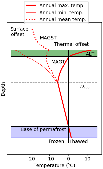
Figure 1 Schematic of the mean, minimum and maximum annual temperature profile from the surface boundary layer to below the bottom of the permafrost. MAAT is the mean annual air temperature; MAGST is the mean annual ground surface temperature at 0.2 m; MAGT is the temperature at the top of the permafrost; ALT is the seasonal thaw depth in any given year. The surface offset is the difference between the MAAT and the MAGST, and the thermal offset is the difference between the MAGST and the MAGT. D_zaa is the depth of zero annual amplitude of ground temperature.

The summer thaw depth depends strongly on the incoming solar radiation as well as on soil moisture, soil organic content and topography and responds to short-term climate variations (Karjalainen et al., 2019). In particular, soils with a higher ice content thaw more slowly than those with lower ice content, resulting in a shallower maximum thaw depth or ALT. Gradual thaw will occur as the global temperature increases, leading to an increase in both the ALT and the time over which the near-surface soil is thawed. These two factors can be represented jointly by the annual mean thawed fraction of the soil (Harp et al., 2016), which can also be used as a proxy for the soil carbon exposure to decomposition. Abrupt thaw processes caused by the melting of excess ground ice will also occur with the landscape destabilising and collapsing (Turetsky et al., 2020). These thermokarst processes are not currently represented in earth system models and are not assessed here.

This paper evaluates the ability of the CMIP6 models to represent present-day permafrost dynamics in terms of the presence or absence of permafrost, the mean annual ground temperature (MAGT), the maximum active layer thickness (ALT) and the annual mean thawed fraction. This is accompanied by an analysis of the improvement in the models' structure when compared with the CMIP5 multi-model ensemble. Finally the simulated sensitivity to climate change of northern high-latitude soils is quantified in order to explore their potential fate in the future and any consequent climate impacts.

2 Materials and methods

2.1 CMIP model data

Historical and future monthly mean data were retrieved for a subset of coupled climate models from the CMIP6 (Eyring et al., 2016; Table 1) and the CMIP5 (Taylor et al., 2012; Table S2.1 in the Supplement) model archive. The historical simulations run from 1850∕60 to the end of 2014 (CMIP5 – to end of 2005). The CMIP5 future simulations are based on representative concentration pathways (RCPs; Taylor et al., 2012) which combine scenarios of land use and emissions to give a range of future outcomes through to 2100. When available, RCP8.5 (high pathway), RCP4.5 (intermediate pathway) and RCP2.6 (peak and decline pathway) are used here. The CMIP6 projections (O'Neill et al., 2016) are based on scenarios that combine shared socioeconomic pathways (SSPs) with updated RCPs. The most widely used scenarios are SSP5-8.5 (a fossil-fuel-intensive development socio-economic pathway, updating RCP8.5), SSP3-7.0 (a “regional rivalry” SSP with unmitigated fossil fuel emissions at the medium to high end of the range), SSP2-4.5 (a “middle of the road” SSP with an emission scenario updating RCP4.5) and SSP1-2.6 (a sustainable pathway with low-end emissions, updating RCP2.6).

Monthly diagnostics processed are surface air temperature (tas; equivalent to 2 m temperature), snow depth (snd), and vertically resolved soil temperatures (tsl) for latitudes greater than 20^∘ N for the first ensemble member of each model where available (i.e. simulation r1i1p1 or similar). Each model is left at its native grid. In addition, grid cells with exposed ice or glaciers at the start of the historical simulation are masked out and the land fractions in the models are accounted for in any area-based assessment of permafrost.

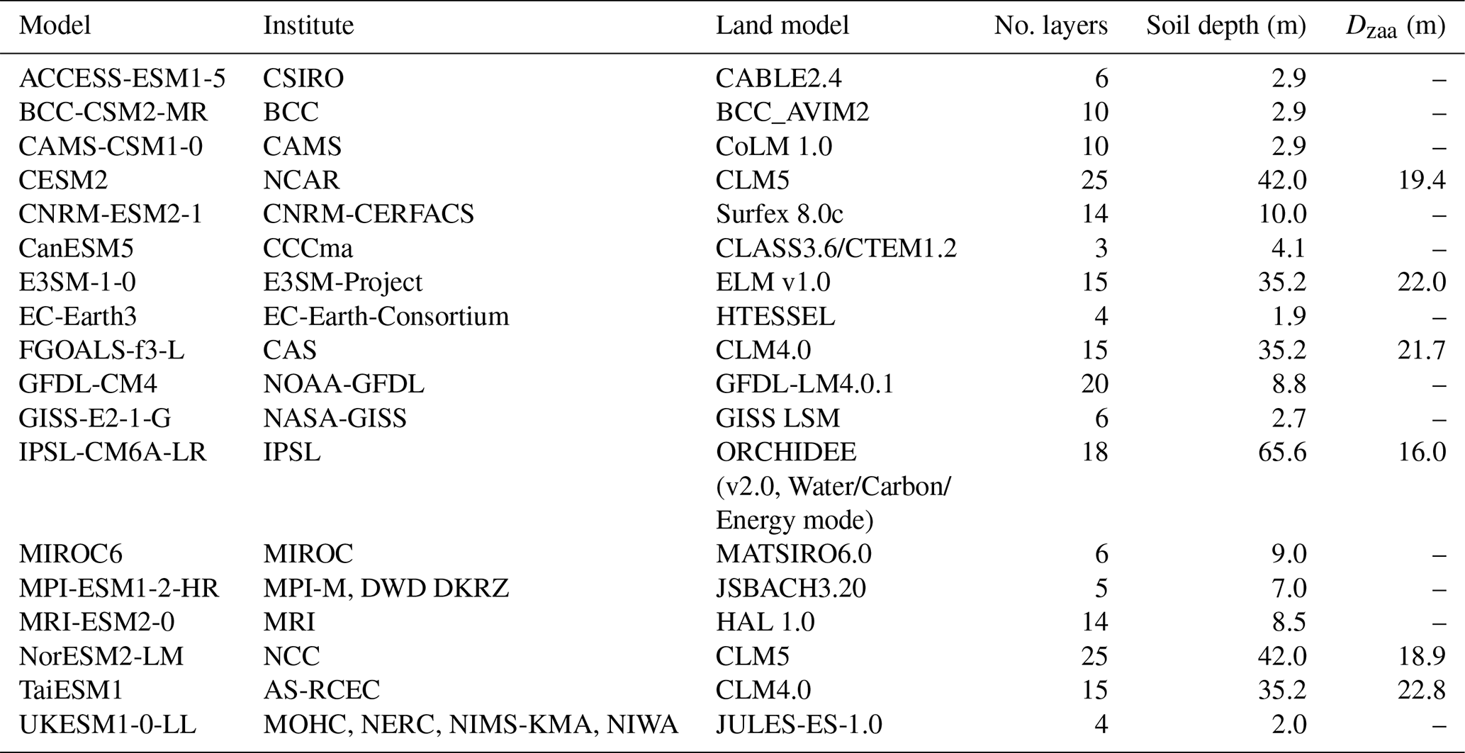
Table 1 A summary of the CMIP6 models used in this study including the number of soil layers and the depth of the middle of the bottom soil layer. Also show is D_zaa for the models where the difference in the annual maximum and minimum soil temperatures at the maximum soil depth is less than 0.1 ^∘C. CMIP5 models are summarised in Table S2.1.

2.2 Observational-based data sets

2.2.1 Air temperature

Air temperature observations over land at 2 m were taken from the WATCH Forcing Data methodology applied to the ERA-Interim (WFDEI) data set (Weedon et al., 2014). These were generated by applying monthly bias corrections from Climatic Research Unit (CRU; Mitchell and Jones, 2005) to the Era-Interim reanalysis data (ECMWF, 2009). Air temperatures are available at 0.5^∘ resolution and were aggregated to monthly and annual means.

2.2.2 Large-scale snow depth product

This data set consists of a Northern Hemisphere subset of the Canadian Meteorological Centre (CMC) operational global daily snow depth analysis (Brown and Brasnett, 2010). The analysis is performed using real-time, in situ daily snow depth observations and optimal interpolation with a first-guess field generated from a simple snow accumulation and melt model driven with temperatures and precipitation from the Canadian forecast model. The analysed snow depths are available at approximately 24 km resolution for the period between 1998 and 2016 and were converted from daily to monthly means. It should be noted that snow depths exhibit high spatial variability and are difficult to measure because of land surface heterogeneity. In addition there are few evaluation data available for the Arctic.

2.2.3 Permafrost extent

The International Permafrost Association (IPA) map of permafrost presence (Brown et al., 1998) gives a historical permafrost distribution compiled for the period between 1960 and 1990. It separates continuous (90 %–100 %), discontinuous (50 %–90 %), sporadic (10 %–50 %) and isolated (< 10 %) permafrost. This distribution was generated from the original 1:10 000 000 paper map, and the version used here was regridded to a 0.5^∘ resolution.

The ESA Climate Change Initiative permafrost (CCI-PF) reanalysis data set (Obu et al., 2019) is a recently developed data set that supplies the mean annual ground temperature at the top of the permafrost (MAGT) and the probability of permafrost for each grid cell. These were derived from an equilibrium model of permafrost at 1 km resolution and provide a snapshot of the 2000–2016 period. The model is driven by remotely sensed land surface temperatures, downscaled ERA-Interim climate reanalysis data, tundra wetness classes and a land cover map. These data were within $\sim \pm \mathrm{2}$ ^∘C of in situ borehole measurements. This CCI-PF analysis of permafrost extent is within the range of but slightly lower than the estimate of Brown et al. (1998). We use a version of the CCI-PF which has been regridded to a 0.5^∘ resolution.

An alternative way of deriving an observational-based estimate of permafrost presence is to derive the probability of permafrost from the observed mean annual air temperature (MAAT). An observational-based relationship was defined by Chadburn et al. (2017), who updated Gruber (2012). The Chadburn et al. (2017) relationship has a 50 % chance of the presence of permafrost at −4.3 ^∘C. Using the Chadburn et al. (2017) relationship, we reconstructed a permafrost probability map from the WFDEI estimates of MAAT. In addition we applied the Chadburn et al. (2017) relationship to the MAAT for each model to estimate a benchmark permafrost distribution specific to each model (PF_benchmark). This model-specific PF_benchmark can be used to evaluate the land surface module independently of any climate biases in MAAT.

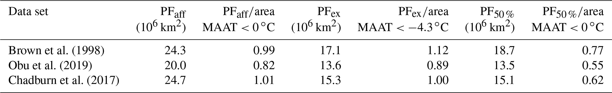
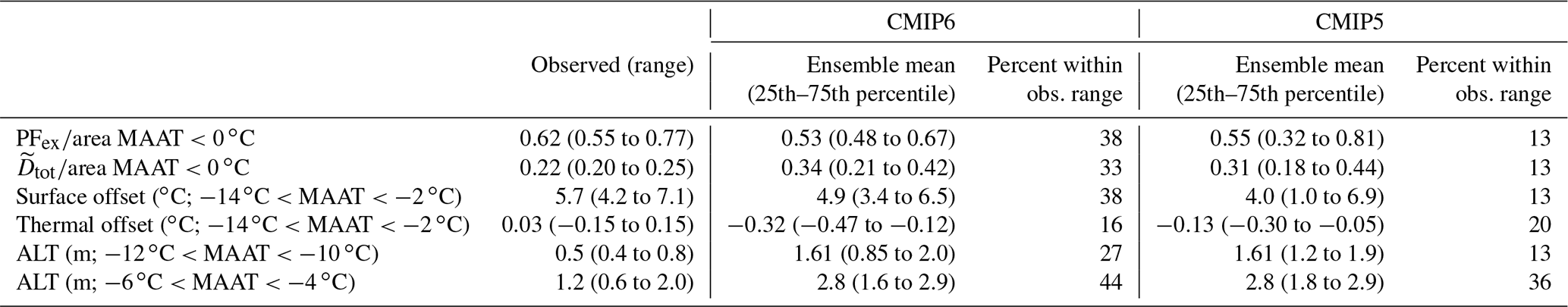
Table 2 summarises the different observational-based permafrost distributions. The permafrost-affected area (PF_aff) is defined as the area where the probability of permafrost is greater than 0.01 and is expected to be very similar to the land surface area where the MAAT is less than 0 ^∘C. Table 2 shows that this is the case for the Brown et al. (1998) and Chadburn et al. (2017) data set, but the Obu et al. (2019) CCI-PF data set has a slightly lower PF_aff area. It should be noted that the Brown et al. (1998) observational data set was one of the data sets used to develop the Chadburn et al. (2017) relationship but the Obu et al. (2019) CCI-PF reanalysis data set was developed independently. The permafrost extent (PF_ex) is the area of permafrost weighted by the proportion of permafrost in each grid cell, and PF_50 % is the area of the grid cells where the probability of finding permafrost is greater than 0.5. These two definitions produce a very similar land surface area. Overall there is some uncertainty in the proportion of the land surface with MAAT<0 ^∘C that contains permafrost – the observational estimates are 0.55, 0.62 and 0.77. The Brown et al. (1998) data have a similar value for the PF_aff area but a higher probability of finding permafrost at air temperatures less than −4.3 ^∘C. Overall the CCI-PF data (Obu et al., 2019) show consistently less permafrost (Table 2).

Table 2 Permafrost areas from three of the available observational data sets defined both as an areal extent and as a fraction of the area where the observed MAAT is below the given threshold. PF_aff is defined as the permafrost-affected area and includes any grid cells which have a non-zero probability (>1 %) of permafrost occurrence. PF_ex is the area of permafrost weighted by the proportion of permafrost in each grid cell, and PF_50 % is the area where the probability of finding permafrost is ≥50 %. The Chadburn et al. (2017) relationship has a 50 % chance of the presence of permafrost at −4.3 ^∘C. MAAT is the mean for the period 1995 to 2014.

2.2.4 Site-specific observations

The Circumpolar Active Layer Monitoring Network (CALM; Brown, 1998) is a network of over 100 sites at which ongoing measurements of the end-of-season thaw depth or the ALT are taken. Measurements are available from the early 1990s, when the network was formed, to the present.

MAAT, MAGT, snow depth and MAGST (mean annual ground surface temperature at 0.2 m) were available for a range of sites in Russia and Canada (Zhang et al., 2018). The data at Russian meteorological stations are from the All-Russian Research Institute of Hydrometeorological Information – World Data Center (RIHMI-WDC), and data at Canadian climate stations are from Environment and Climate Change Canada. This gives data from ∼330 stations (Sherstiukov, 2012). Additional data are available from the Global Terrestrial Network for Permafrost (GTN-P; Biskaborn et al., 2015, 2019). Ground temperatures are measured in >1000 boreholes at a wide variety of depths. Years with a complete seasonal cycle were extracted from selected boreholes where the data available include MAAT, MAGST and MAGT. A full description of these data and their post-processing is included in Zhang et al. (2018).

2.3 Evaluation metrics

These metrics are derived from both the models and the observations in a consistent manner.

2.3.1 Effective snow depth

Snow has a big impact on the soil temperatures and presence or absence of permafrost in the northern high latitudes (Wang et al., 2016; Zhang, 2005). Here we use the effective snow depth, S_depth,eff (Slater et al., 2017) which describes the insulation of snow over the cold period. S_depth,eff is an integral value such that the mean snow depth in each month, m (S_m in metres) is weighted by its duration:

$$\begin{array}{}\text{(1)}& {\displaystyle }{\displaystyle }{S}_{\text{depth,eff}}={\displaystyle \frac{{\sum }_{m=\mathrm{1}}^M{S}_m(M+\mathrm{1}-m)}{{\sum }_{m=\mathrm{1}}^{M}m}}.\end{array}$$

It is assumed that the snow can be present anytime from October (m=1) to March (m=6) with the maximum duration, M, equal to 6 months. This weights early snowfall more than late snowfall as it will have a greater overall insulating value. The insulation capacity of the snow changes little with snow depth when S_{depth, eff} increases above ∼0.25 m (Slater et al., 2017), and seasons with an earlier snowfall will generally have a greater S_depth,eff than seasons with a later snowfall.

2.3.2 Winter, summer and thermal offsets

The winter offset is defined as the difference between the mean soil temperature at 0.2 m and the mean air temperature for the period from December to February. This is expected to be positive with the soil temperature warmer than the air temperature. The summer offset is defined in a similar manner for the period between June and August. This is expected to be slightly negative with the soil temperature cooler than the air temperature. The surface offset is the sum of the summer and winter offset but is dominated by the winter offset. The thermal offset is the temperature difference between the annual mean soil temperature at 0.2 m (mean annual ground surface temperature – MAGST) and the annual mean soil temperature at the top of the permafrost (mean annual ground temperature – MAGT). This is expected to be slightly negative with MAGT slightly colder than MAGST.

2.3.3 Diagnosing permafrost in the model

In this paper the preferred method of defining permafrost is to diagnose the temperature at the depth of zero annual amplitude (D_zaa). D_zaa is defined as the minimum soil depth where the variation in monthly mean temperatures within a year is less than 0.1 ^∘C. If the temperature at the D_zaa is less than 0 ^∘C for a period of 2 years or more, there is assumed to be permafrost in that grid cell. However, only six of the CMIP6 models have a soil profile deep enough to identify the D_zaa (Table 1). In the remainder of the models, the maximum soil depth is less than the D_zaa, so an alternative method of identifying the presence of permafrost is required. For these models permafrost is assumed to be present in grid cells where the 2-year mean soil temperature of the deepest model level is less than 0 ^∘C. This definition was used by Slater and Lawrence (2013), who suggested that if the mean soil temperature of the deepest model level is below 0 ^∘C and assuming constant soil heat capacity, there is likely to be permafrost deeper in the soil profile. However, this definition does not explicitly recognise permafrost in the soil profile – in order to do that, the maximum soil temperature of the deepest model level should be less than 0 ^∘C. The main issue with this latter method is that, if the soil profile does not extend deep enough, the deepest model level may fall in the ALT and the permafrost extent will be underestimated.

Subgrid-scale variability is not taken into account in this assessment – the models are assumed to have either permafrost or no permafrost in each grid cell. However, the observations either are very high resolution (CCI-PF is at 1 km resolution in its original format) or supply a probability of permafrost for each grid cell (Brown et al., 1998; Chadburn et al., 2017). Therefore in order to compare the observed extent with those from the models, we assume that any grid cell where the observations have ≥50 % permafrost should be identified by the models as having permafrost and any grid cells with <50 % will be identified as not having permafrost. The observed values of this threshold (PF_50 %) are shown in Table 2 and are approximately equal to the permafrost extent (PF_ex, also shown in Table 2), which is defined as the observed area of permafrost which takes into account the proportion of permafrost in each of the grid cells.

2.3.4 Thaw depth and associated metrics

The thawed depth from the surface is defined for each month using the depth-resolved monthly mean soil temperatures. The soil temperatures were interpolated between the centre of each model level and the thaw depth defined at the minimum depth where it reaches 0 ^∘C. Some of the models have a very poorly resolved soil temperature profile which will introduce some biases into this estimate (Chadburn et al., 2015). In addition, taliks (unfrozen patches within the frozen part of the soil) will not be identified using this method. The annual maximum active layer thickness (ALT in metres) is defined as the maximum monthly thaw depth for that year.

Under increasing temperature both the ALT and the time the soil is thawed will increase via an earlier thaw and later freeze up. Therefore, Harp et al. (2016) defined the annual mean thawed fraction ($\stackrel{\mathrm{̃}}{D}$) for permafrost soils which can be expressed in units of cubic metres per cubic metre:

$$\begin{array}{ll}{\displaystyle }& {\displaystyle }\stackrel{\mathrm{̃}}{D}={\displaystyle \frac{\mathrm{1}}{z_{\text{max}}}}{\displaystyle \frac{\mathrm{1}}{\mathrm{12}}}\underset{\mathrm{1}}{\overset{\mathrm{12}}{\int }}\underset{\mathrm{0}}{\overset{z_{\text{max}}}{\int }}H\left(T\right(z,t\left)\right)\mathrm{d}z\mathrm{d}t,\\ \text{(2)}& {\displaystyle }& {\displaystyle }H\left(T\right(z,t\left)\right)=\left\{\begin{array}{ll}\mathrm{1}& \text{if }T(z,t)>\mathrm{0},\\ \mathrm{0}& \text{if }T(z,t)\le \mathrm{0},\end{array}\right.\end{array}$$

where t is the time in months, z is the depth in metres, T is the soil temperature at time t and depth z, and z_max is the maximum depth of the soil under consideration. Here we assume z_max is 2 m which is relatively shallow but enables the models with shallower soil depths to be included consistently within the analysis. The annual mean frozen fraction ($\stackrel{\mathrm{̃}}{F}$) is the frozen component of the soil and given by

$$\begin{array}{}\text{(3)}& {\displaystyle }{\displaystyle }\stackrel{\mathrm{̃}}{F}=\mathrm{1}-\stackrel{\mathrm{̃}}{D}.\end{array}$$

One advantage of using $\stackrel{\mathrm{̃}}{D}$ over ALT is that it enables taliks to be identified, although this will become more relevant when considering soils deeper than 2 m. In addition, $\stackrel{\mathrm{̃}}{D}$ is a first-order proxy for the soil carbon exposure to decomposition in any particular grid cell.

The annual thawed volume (${\stackrel{\mathrm{̃}}{D}}_{\text{tot}}$ in cubic metres) is the sum of the area-weighted values of $z_{\text{max}}\stackrel{\mathrm{̃}}{D}$ for each grid cell in the present-day permafrost region. Any non-permafrost grid cells are masked. Similarly the annual frozen volume (${\stackrel{\mathrm{̃}}{F}}_{\text{tot}}$ in cubic metres) is the sum of the area-weighted $z_{\text{max}}\stackrel{\mathrm{̃}}{F}$ for each grid cell again defined for the present-day permafrost region. For any future projections, if there is no longer freezing in a specific grid cell (which had permafrost in the present day), $\stackrel{\mathrm{̃}}{D}$ is set to 1 and $\stackrel{\mathrm{̃}}{F}$ is set to 0.

We can derive an observational-based estimate of present-day ${\stackrel{\mathrm{̃}}{D}}_{\text{tot}}$ using the available site-specific data between $\stackrel{\mathrm{̃}}{D}$ and MAGT described in Sect. 2.2.4 and shown in Fig. 2. The CCI-PF data set was then used in conjunction with this relationship to estimate $\stackrel{\mathrm{̃}}{D}$ over the permafrost region. $\stackrel{\mathrm{̃}}{D}$ is related non-linearly to the MAGT – the warmer the ground temperature, the bigger the annual mean thawed fraction. Therefore a second-order polynomial was fitted to the site-specific relationship between $\stackrel{\mathrm{̃}}{D}$ and the MAGT – green line in Fig. 2. The dashed black lines show the relationship for the 95 % confidence intervals. These three curves were then used in conjunction with the CCI-PF data set to derive the mean and range of $\stackrel{\mathrm{̃}}{D}$ for each grid cell with permafrost present. Assuming z_max is 2 m and summing over the CCI-PF permafrost area give a present-day ${\stackrel{\mathrm{̃}}{D}}_{\text{tot}}$ of 5.6×10³ km³ (range 2.1–9.5×10³ km³). ${\stackrel{\mathrm{̃}}{F}}_{\text{tot}}$ is then 22.2×10³ km³ (range 18.4–25.8×10³ km³).

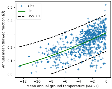
Figure 2 The relationship between the MAGT and $\stackrel{\mathrm{̃}}{D}$ for observed sites and years where both monthly thaw depths and MAGT are available (Zhang et al., 2018). The solid green line is the best fit, and the dashed black lines are the 95 % confidence intervals.

3 Results

In a global climate model the permafrost dynamics are affected by both the driving climate and the parameterisations used to translate the meteorology into the presence or absence of permafrost, namely the land surface module. Here we separate out these two factors and, where possible, identify the relative uncertainties introduced.

3.1 Driving climate

Figure 3 shows the differences between the observations and the CMIP6 models for relevant climate-related characteristics of the permafrost-affected region (PF_aff) defined by the CCI-PF data (Table 2). The horizontal grey lines in Fig. 3 represent ±15 % of the observed value. Absolute values for individual models and the observations are given in Table S1.1. These can also be compared with the CMIP5 multi-model ensemble (Fig. S2.1 and Table S2.2 in the Supplement).

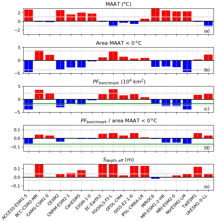
Figure 3 The climate characteristics of the CMIP6 multi-model ensemble compared with the observations for the period 1995–2014. The air temperature observations are from Weedon et al. (2014); the PF_benchmark observations are from Chadburn et al. (2017); and the S_depth,eff observations are from Brown and Brasnett (2010). The red bars are where the model value is greater than the observations, and the blue bars are where the model value is less than the observations. S_depth,eff is for the period 1998–2016 and has not been uploaded to the CMIP archive for every model. The green lines represent the difference between the Chadburn et al. (2017) data set and the Obu et al. (2019) CCI-PF data (Table 2).

The MAAT is, to first order, the driver of the presence or absence of permafrost (Chadburn et al., 2017). The ability of the climate models to correctly simulate the northern high latitudes' MAAT is assessed in Fig. 3a and b. The CMIP6 models tend to be biased warm compared with the observations, and the area where the land surface temperature is less than 0 ^∘C is biased low. However, in general the models fall within ±2 ^∘C of the observed MAAT (−6.8 ^∘C) and within $\pm \mathrm{4.0}\times {\mathrm{10}}^{\mathrm{6}}$ km² of the observed area where MAAT is less than 0 ^∘C (24.4×10⁶ km²). These inter-model differences will be reflected in differences in any estimates of permafrost.

Figure 3c shows how biases in the models' MAAT impact the presence of permafrost when permafrost is derived from the MAAT using the Chadburn et al. (2017) relationship (PF_benchmark). PF_benchmark ranges between 11.0 and 18.97×10⁶ km² (Table S1.2), and the models are fairly equally distributed around the observational-based value of 15.1×10⁶ km². The green line represents the difference between the Chadburn et al. (2017) observations and the CCI-PF data. Overall the CCI-PF data have less permafrost than both the Chadburn et al. (2017) observations and the majority of models. The differences between models appear smaller when PF_benchmark is normalised by the area where MAAT is less than 0 ^∘C. These values range between 0.58 and 0.68 (Table S1.2) compared with 0.62 found from the Chadburn et al. (2017) relationship using WFDEI MAAT. The differences between models shown in Fig. 3d are caused by differences in the latitudinal dependence of MAAT for temperatures between 0 and −7.6 ^∘C – the threshold temperatures of permafrost presence or absence and continuous permafrost respectively suggested by Chadburn et al. (2017).

Figure 4 summarises the CMIP6 multi-model ensemble by showing the multi-model mean probability of permafrost. Panel a defines the permafrost using PF_benchmark. Any region where there is permafrost using this definition is shaded in purple. Superimposed is the contour plot of probability of permafrost from Obu et al. (2019) with the orange lines being the limits of 50 % permafrost. In general the continuous permafrost area is well represented as 100 % permafrost, meaning that all of the models can represent the area of continuous permafrost. However, the permafrost extends further south in a small handful of models, as might be expected from the spread in Fig. 3. Figures for individual models are shown in Fig. S1.1. The PF_benchmark for each model can be used as the reference data for evaluating the ability of the land surface component to appropriately estimate permafrost presence.

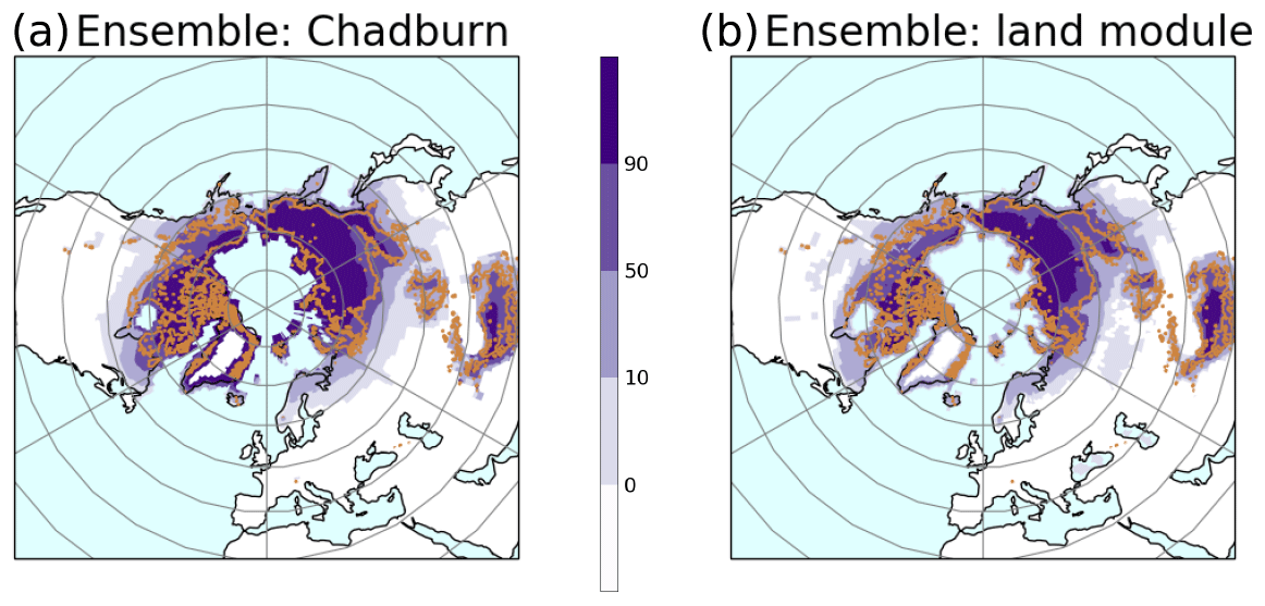
Figure 4 (a) The multi-model probability of permafrost using the Chadburn et al. (2017) relationship for each model (PF_benchmark). (b) The multi-model probability of permafrost where permafrost is defined by the temperature at the D_zaa or the lowest model level for the models with the shallower soil profile (PF_ex). These plots are the mean for 1995–2014. The orange lines are the limits for 50 % permafrost from the CCI-PF data (Obu et al., 2019).

The CMIP6 multi-model ensemble can be compared with the CMIP5 multi-model ensemble (Table 3). The standard time periods are slightly different for each multi-model ensemble: the CMIP6 climatologies are for 1995–2014, and the CMIP5 climatologies are for 1986–2005. Therefore the observed values (except for S_depth,eff which covers a more limited time period) are slightly different with the MAAT for CMIP6 being about 0.3 ^∘C warmer than for CMIP5 and the area where the land surface is less than 0 ^∘C being 0.4×10⁶ km² larger for CMIP5. Overall the two multi-model ensemble means agree with the observations for the metrics derived from air temperature with the majority of the constituent models falling within ±15 % of the observed values. Table 3 shows the CMIP6 models are comparable with the CMIP5 models.

Table 3 A summary of the CMIP6 climate evaluation metrics compared with both the observations and CMIP5. Where relevant, statistics are given for PF_aff defined by CCI-PF (Table 2). The difference between the multi-model ensemble mean and the observations are shown plus the percentage of the multi-model ensemble within ±15 % of the observations. It should be noted that the observed S_depth,eff is for the period 1998–2016.

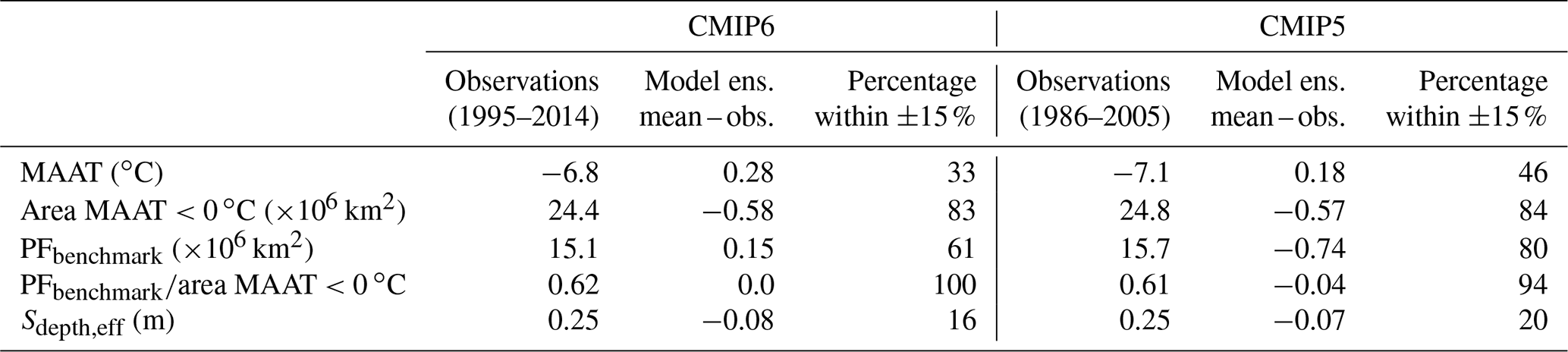
Figure 5 S_depth,eff for 1999–2014 for the multi-model ensemble mean of the CMIP6 models (a) compared with the CMC observations (b). (c) The differences between the multi-model ensemble mean and the observations. All grid cells with S_depth,eff less than 0.02 m are masked.

The precipitation will also affect the presence or absence of permafrost – in particular any snowpack will insulate the soil. The land surface scheme translates snowfall to snow lying on the surface and quantifies its insulating capacity. Therefore biases in both the snow amount and snow physics will influence the snow insulation. The snow amount can be represented by the S_{depth, eff}. Figure 5 shows the multi-model ensemble median S_depth,eff compared with the observations from the CMC snow depth analysis (Brown and Brasnett, 2010) for the time period 1998–2014, and Fig. S1.2 shows S_depth,eff for the individual models. All grid cells with S_depth,eff less than 2 cm are masked. S_depth,eff for the Arctic is generally greater than 0.2 m in the multi-model ensemble mean. The observations have some regions in the northern tundra where the effective snow depth is slightly shallower than 0.2 m which are not reflected on the multi-model ensemble mean or in the individual models. This results in a tendency for the models to slightly overestimate the snow depth in the tundra. The snow region extends further south in the multi-model ensemble mean than in the observations which reflects some of the variability between models. The large spatial variability in snow over the Arctic will not be well represented by either the models or the observations. Individual CMIP6 models (Figs. S1.2 and 3) that notably overestimate the S_depth,eff include BCC-CSM2-MR, EC-Earth3, FGOALS-f3-L, GISS-E2-1-G and IPSL-CM6A-LR. Only 16 % of the models have a mean S_depth,eff within ±15 % of the observations (Table 3). It should be noted that S_depth,eff will be moderated by snow physics and in the case of snow the climate biases cannot be cleanly separated from the land surface biases.

3.2 Land surface module

The land surface modules translate the driving climate into the permafrost dynamics. In effect they quantify the offsets shown in Fig. 1. Figure 6 shows the spread of these offsets as a function of MAAT for the CMIP6 multi-model ensemble along with an estimate of the observed surface and thermal offsets. This spread was calculated independently for each model by binning the MAAT into 0.5 ^∘C bins and calculating the median value of each offset for each bin. The winter offset is by far the largest offset with the largest uncertainty, and it is strongly dependent on MAAT. Therefore snow plays a dominant role in the relationship between MAGT and MAAT. The summer and thermal modelled offsets both have a small negative value, cover a smaller range of values and are only slightly dependent on MAAT. In comparison to the observations and assuming the summer offset is small, the model-simulated winter offsets are possibly slightly too small at the warmer temperatures and slightly too large at the colder temperatures. Figure S1.3 shows the variation is relatively large between the individual models. For example, MPI-ESM1-2-HR has very little difference between the MAAT and the MAGT with all offsets on the order of 1 ^∘C or less; similarly ACCESS-ESM1-5 has a relatively small winter offset. In contrast a few models have very high winter offsets which reach over 10 ^∘C at cold temperatures (UKESM1-0-LL, CAMS-CSM1-0, FGOALS-f3-L and TaiESM1). However, comparing the CMIP5 models with the CMIP6 models (Figs. S1.3 and S2.5) suggests that there has been a general improvement since CMIP5 when compared with the observations.

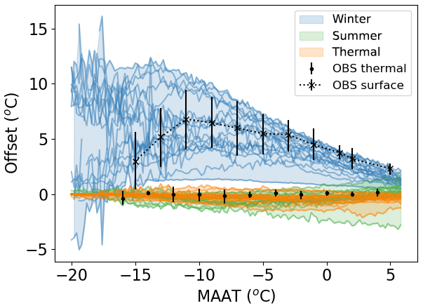
Figure 6 Multi-model ensemble spread of the median winter, median summer and median thermal offsets for the CMIP6 multi-model ensemble. Individual models for the CMIP6 multi-model ensemble are shown as lines and identified in Fig. S1.3 and for the CMIP5 multi-model ensemble in Fig. S2.5. The observed surface and thermal offsets summarised from the available point data (Zhang et al., 2018) are added in black. Although the observed surface offset is not directly comparable with the separate winter and summer offsets, these are shown for the models to illustrate their relative magnitudes.

3.2.1 Mean annual ground temperature

Figure 6 suggests that in order for a land surface module to accurately represent permafrost it needs to be able to represent the insulating ability of the lying snow. This is assessed in Fig. 7 which shows the insulating capacity of the snow in terms of the difference between the winter air temperature and winter 0.2 m soil temperature. The offsets are a function of both MAAT (not shown) and S_{depth, eff}. A low MAAT and a high S_depth,eff gives a bigger offset (see also Wang et al., 2016). In Fig. 7 only grid cells where the winter mean air temperatures are between −25 and −15 ^∘C are shown, similarly to the observed sites. This ensures the comparisons are not biased by differences in air temperatures. The available models reflect the general increase in offset with increasing S_depth,eff for the shallow snow and the saturation of this relationship for the deepest S_depth,eff to varying degrees of accuracy. A few of the models (FGOALS-f3-L, TaiESM1 and UKESM1-0-LL) have relationships between offset and S_{depth, eff} which are indistinguishable from the observed relationship. The rest of the models have an offset at any given S_depth,eff which is generally too small, suggesting that these models do not have enough snow insulation. The net impact of the snow offset needs to be interpreted carefully in combination with the S_depth,eff in order to evaluate the impact of the snow insulation on permafrost dynamics. Figure 5 shows that Arctic snow depths are relatively shallow. Therefore, because there is a non-linear relationship between offset and S_depth,eff, small differences in S_depth,eff will have a big impact on the insulating ability. The models typically tend to slightly overestimate S_depth,eff and slightly underestimate the offset for any given value of S_depth,eff.

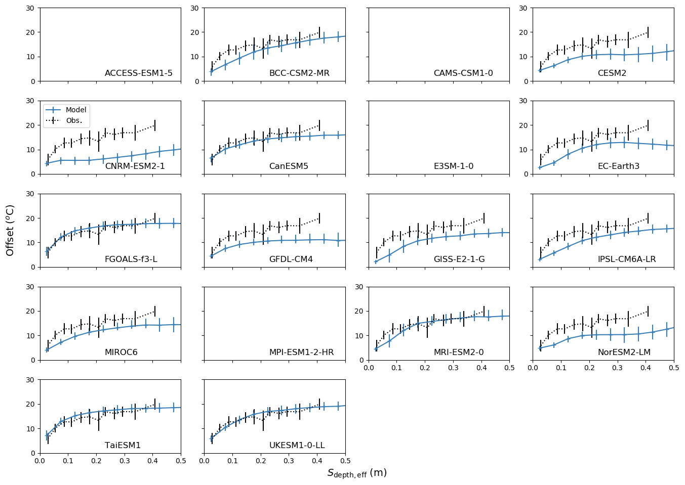
Figure 7 Differences between the air and soil temperature at 0.2 m for the winter as a function of S_depth,eff. Only grid cells or sites where the winter air temperature is between −25 and −15 ^∘C are shown. The climatological period of 1995–2014 is shown for the CMIP6 models. The blue points with the error bars are the model data, and the dotted black lines and error bars are the observations derived using the data from Zhang et al. (2018). In addition, only the models where snow depths are available from the CMIP archives are shown.

Figure S2.6 shows the equivalent plots for the available CMIP5 models. A similar pattern is observed where the models are more likely to underestimate than overestimate the snow insulation. Although limited availability means it is hard to compare individual models between the CMIP5 and CMIP6 ensemble, specific models can be identified. Specifically CanESM and MIROC show improvements; MRI and GISS show little change, and CESM and NorESM show some degradation.

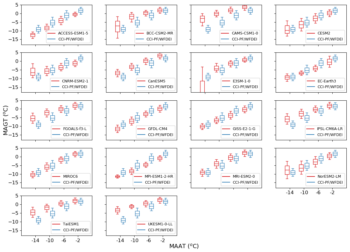
Figure 8 MAGT as a function of local MAAT for the CMIP6 models and the climatological period 1995–2014 (in red). The MAGT observations (in blue) were taken from the CCI-PF data set and the MAAT from the WFDEI data.

Figure 8 shows the combined impact of the three offsets on the relationship between MAGT and MAAT compared with an observational-based assessment made using the CCI-PF MAGT and the WFDEI MAAT. As expected the MAGT increases with MAAT, with the CCI-PF MAGT approximately 4.5 ^∘C warmer than the WFDEI MAAT. As discussed earlier, this difference is dominated by the winter offset, but the summer and thermal offsets also contribute. Also shown are the same relationships for the models. Differences in snow insulation are reflected here. For example, despite recreating the observed relationship between winter offset and S_depth,eff, the BCC-CSM2-MR and UKESM1-0-LL models have a much larger difference between MAAT and MAGT than the observations at the colder temperature, because there is too much snow on the ground in the high Arctic. CESM2 has a very similar relationship between MAAT and MAGT to the observations (Fig. 8) despite having a smaller winter offset than is observed for any given value of S_depth,eff (Fig. 7). However, it has a larger-than-observed S_depth,eff which increases the insulation and ensures a good relationship between MAAT and MAGT in Fig. 8. A comparison with the CMIP5 multi-model ensemble (Fig. S2.7) shows similar differences. It should be noted that this CCI-PF estimate of MAGT is a model-derived reanalysis and the observational uncertainties are likely underestimated in the current analysis.

3.2.2 Active layer thickness

An assessment of the thaw depth of the permafrost during the summer gives another indication of whether the model has the correct physics. Differences between the model and observations are apparent in Fig. 9. The observed relationship between the ALT and the MAAT in the CALM data set is shown in blue. Both the observed ALT and the spread of possible ALT increase with increasing MAAT. The spread of values increases because the active layers are more strongly impacted by environmental factors other than air temperature such as topography, soil type and solar radiation at the warmer temperatures. For each model the percentage of observed CALM sites where there is model-simulated permafrost is shown in the figure. The maximum observed ALT is about 4.5 m. Any models with a maximum soil depth of less than 4.5 m will be unable to represent this value (Table 1). This is the case for GISS-E2-1-G, where the depth of the middle of the bottom layer is 2.7 m and the ALT is constrained to 2.7 m at the warmer temperatures. Poor vertical discretisation of the soil such as the three layers in CanESM5 can introduce large variability into the derivation of ALT. Although the average number of soil layers and the average soil depth increases between the CMIP5 and CMIP6 ensembles (CMIP6 – Table 1; CMIP5 – Table S2.1), this is not universally true.

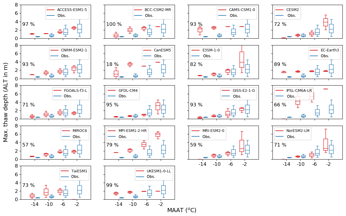
Figure 9 Active layer thickness (ALT) as a function of local MAAT for the CMIP6 models (in red) and the climatological period 1995–2014. Observations of the active layer (in blue) are from the CALM sites, and the air temperatures are from the large-scale WFDEI data set. The percentage of the observed sites which also have permafrost in the models is shown in each subplot.

About half of the models have relationships between ALT and MAAT that are comparable with the observations. These are mainly the models with deeper soils. Other models have a very deep ALT, for example, MPI-ESM1-2-HR and IPSL-CM6A-LR. These both have sufficiently deep soil profiles but thaw too quickly in the summer, likely because these models do not represent the latent heat of the water-phase change. EC-Earth3 and UKESM1-0-LL have active layers around 2 m irrespective of MAAT. In the case of UKESM1-0-LL, this is worse than the CMIP5 version of the model where ALT was dependent on MAAT, just with a smaller uncertainty range (Fig. S2.8). This is because there is a large increase in the MAGT between the CMIP versions (MAGT is −5.8 ^∘C for CMIP5 and MAGT and −0.9 ^∘C for CMIP6) caused by adding a multilayered snow scheme (Walters et al., 2019). The inclusion of organic soils and the addition of a moss layer improve the insulating capacity and ability of the soil to hold water and will reduce this thaw depth (Chadburn et al., 2015).

3.2.3 Permafrost extent, annual thawed volume (${\stackrel{\mathrm{̃}}{D}}_{\text{tot}}$) and annual frozen volume (${\stackrel{\mathrm{̃}}{F}}_{\text{tot}}$)

MAGT and ALT and their relationships with MAAT are important diagnostics for model physics. However, permafrost extent and annual thawed and frozen volume are more relevant when exploring the impacts of permafrost dynamics under future climate change. There are observational-based estimates of permafrost extent (Brown et al., 2003; Obu et al., 2019; Chadburn et al., 2017) available for evaluation, and this paper introduces an observational-based estimate of annual thawed and frozen volume by extrapolating the site-specific relationship between annual mean thawed fraction ($\stackrel{\mathrm{̃}}{D}$) and MAGT to the larger scale using the CCI-PF data set.

Figure 10 shows that the relationship between annual mean thawed fraction ($\stackrel{\mathrm{̃}}{D}$) and MAGT for the available CALM and GTNP data sets is relatively well constrained. As expected, $\stackrel{\mathrm{̃}}{D}$ increases with increasing MAGT. Figure 10 also shows the ability of the models to replicate this relationship. At the warmer temperatures the models tend to show much more variability than the observations. In models such as EC-Earth3 and UKESM1-0-LL this is likely reflecting the sensitivity to the duration over which the soil is thawed – because in these models the ALT is very similar at all temperatures (Fig. 9). Overall the models follow a similar trend of increasing $\stackrel{\mathrm{̃}}{D}$ with increasing MAGT. There are notable discrepancies for IPSL-CM6A-LR and MPI-ESM1-2-HR which might be expected because these two models simulate very deep ALT. $\stackrel{\mathrm{̃}}{D}$ can be converted to annual thawed and frozen volumes (${\stackrel{\mathrm{̃}}{D}}_{\text{tot}}$ and ${\stackrel{\mathrm{̃}}{F}}_{\text{tot}}$) using the monthly profiles of modelled soil temperature and compared with the observational-based estimate of ${\stackrel{\mathrm{̃}}{D}}_{\text{tot}}$ and ${\stackrel{\mathrm{̃}}{F}}_{\text{tot}}$ discussed in Sect. 2.3.4. Figure 11 summarises PF_ex, ${\stackrel{\mathrm{̃}}{D}}_{\text{tot}}$ and ${\stackrel{\mathrm{̃}}{F}}_{\text{tot}}$ for each of the CMIP6 models.

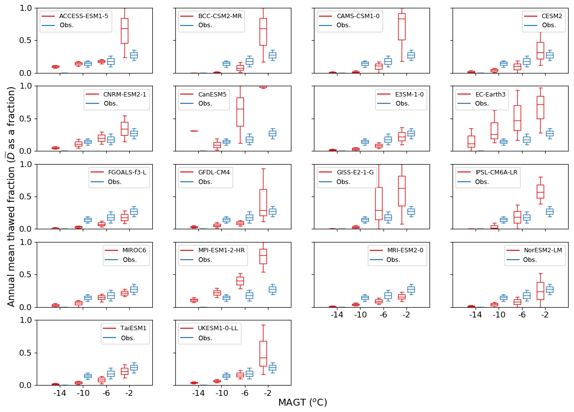
Figure 10 Relationship between the annual mean thawed fraction ($\stackrel{\mathrm{̃}}{D}$) and the MAGT from the site observations and the models in CMIP6 for the climatological period 1995–2014.

The top plot of Fig. 11 shows a comparison of PF_benchmark with the observations (empty black bars). All the models fall close to the observed values, as is expected from Table S1.2. PF_ex (red bar) should be compared with PF_benchmark and not the observations, and any differences between the two quantify a bias added by the land surface model. Any differences here are again dominated by the snow insulation, which is a combination of the S_depth,eff and the relationship between MAGST, MAAT and S_depth,eff. When compared with the CMIP5 multi-model ensemble (Fig. S2.10), the spread of values is smaller, with the differences between PF_ex and PF_benchmark significantly lower in some cases. Assessing Fig. 11 in conjunction with Figs. S1.2 and 7 suggests some improvement in snow insulation between the CMIP5 multi-model ensemble and the CMIP6 multi-model ensemble.

Figure 11 also shows ${\stackrel{\mathrm{̃}}{D}}_{\text{tot}}$ and ${\stackrel{\mathrm{̃}}{F}}_{\text{tot}}$ for each CMIP6 model. These metrics are calculated for the present-day permafrost region defined by the model-specific PF_ex. Any differences between models are caused by a combination of differences in the MAGT and differences in the relationships between $\stackrel{\mathrm{̃}}{D}$ and MAGT. These lead to the considerable spread in ${\stackrel{\mathrm{̃}}{D}}_{\text{tot}}$ and ${\stackrel{\mathrm{̃}}{F}}_{\text{tot}}$ shown in Fig. 11. There is a tendency for the models to overestimate ${\stackrel{\mathrm{̃}}{D}}_{\text{tot}}$ and underestimate ${\stackrel{\mathrm{̃}}{F}}_{\text{tot}}$. This arises partly because of the higher likelihood of the larger values of $\stackrel{\mathrm{̃}}{D}$ at the warmer air temperatures, i.e. in the discontinuous and sporadic permafrost (Fig. 10). The CMIP6 multi-model ensemble has a similar uncertainty to that of CMIP5, suggesting little improvement in the quantification of ${\stackrel{\mathrm{̃}}{D}}_{\text{tot}}$ and ${\stackrel{\mathrm{̃}}{F}}_{\text{tot}}$ between ensembles.

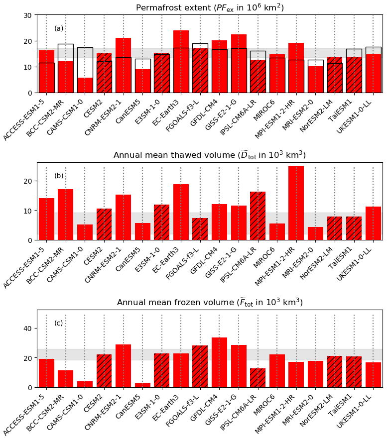
Figure 11 (a) Modelled permafrost extent; (b) annual thawed volume (${\stackrel{\mathrm{̃}}{D}}_{\text{tot}}$); and (c) and annual frozen volume (${\stackrel{\mathrm{̃}}{F}}_{\text{tot}}$) of the top 2 m soil for different CMIP6 models for the climatological period of 1995–2014. Permafrost extents (PF_ex) derived using the mean temperature at D_zaa are the red with black hatching, and those derived using mean temperature at the bottom of the modelled soil profile are in red without hatching. The empty bars with black outlines are the PF_benchmark derived from the relationship of Chadburn et al. (2017). The grey shaded area is the range expected from observations.

3.2.4 Evaluation metrics

This section summarises some basic evaluation metrics which can be applied to quantify the ability of the land surface modules to represent permafrost dynamics. Relevant climate-related metrics are summarised in Table 3 and shown in Table S1.1 for individual CMIP6 models and Table S2.2 for individual CMIP5 models. Table 4 shows a summary of the land-related evaluation metrics for the observations and the two different multi-model ensembles along with the percentage of each multi-model ensemble falling within the range with individual models shown in Tables S1.2 and S2.3. These metrics should be relatively independent of climate and reflect the behaviour of the land surface module. Of particular note is the ALT, a key metric when simulating permafrost dynamics, which is much deeper than the observations for both CMIP5 and CMIP6.

There is better agreement with the observations for the climate-related metrics (Table 3) than for the land-surface-related metrics with only a very small number of models falling within the range of the observations. In addition, there is no consistency in model performance – no model performs well for every evaluation metric (Tables S1.2 and S2.3). Overall, the percentage of the models which fall within the observed range is relatively low with the majority falling outside the range of the observations (Table 4). However, there are some improvements for all the metrics in the percentage of models that fall within the observed range between the CMIP5 multi-model ensemble and the CMIP6 multi-model ensemble.

Table 4 CMIP6 model evaluation metrics summary compared with observations and CMIP5. Individual CMIP6 models are in Tables S1.2 and S2.3.

3.3 Future projections

This paper makes future projections of PF_benchmark, PF_ex, ${\stackrel{\mathrm{̃}}{D}}_{\text{tot}}$ and ${\stackrel{\mathrm{̃}}{F}}_{\text{tot}}$ as a function of global surface air temperature change (GSAT). The results are shown in Fig. 12 for all of the available SSP scenarios. PF_benchmark depends solely on the projections of air temperature; PF_ex depends on the annual mean soil temperature at the lowest model level or D_zaa; and ${\stackrel{\mathrm{̃}}{D}}_{\text{tot}}$ and ${\stackrel{\mathrm{̃}}{F}}_{\text{tot}}$ depend additionally on the thawed component of the soil. We assume the results are scenario independent and calculate the mean of each of the diagnostics for each model after binning into 0.1 ^∘C global surface air temperature bins. Anomalies are then calculated with respect to the values where the GSAT change is 0.0 ^∘C. Data are excluded any time the simulated permafrost extent falls below 1.0×10⁶ km². For most of the models these relationships are approximately linear for temperature changes up to around 3 ^∘C.

The sensitivity of PF_benchmark to increasing GSAT shows a loss of between 3.1 and 3.8×10⁶ ${\mathrm{km}}^{\mathrm{2}}{}^{\circ }{\mathrm{C}}^{-\mathrm{1}}$ (25th to 75th percentile; Table 5) in the CMIP6 multi-model ensemble. This derivation of PF_benchmark uses the observed relationship between MAAT and the probability of permafrost from Chadburn et al. (2017) and assumes it is for an equilibrium state. Therefore this sensitivity is highly dependent on the Arctic amplification in the models. The variability in PF_benchmark between the different models and different multi-model ensembles is relatively small with no obvious outliers. The sensitivities fall to the lower end of the equilibrium sensitivity proposed by Chadburn et al. (2017), who present a loss of ${\mathrm{4.0}}_{-\mathrm{1.1}}^{+\mathrm{1.0}}\times {\mathrm{10}}^{\mathrm{6}}$ ${\mathrm{km}}^{\mathrm{2}}{}^{\circ }{\mathrm{C}}^{-\mathrm{1}}$.

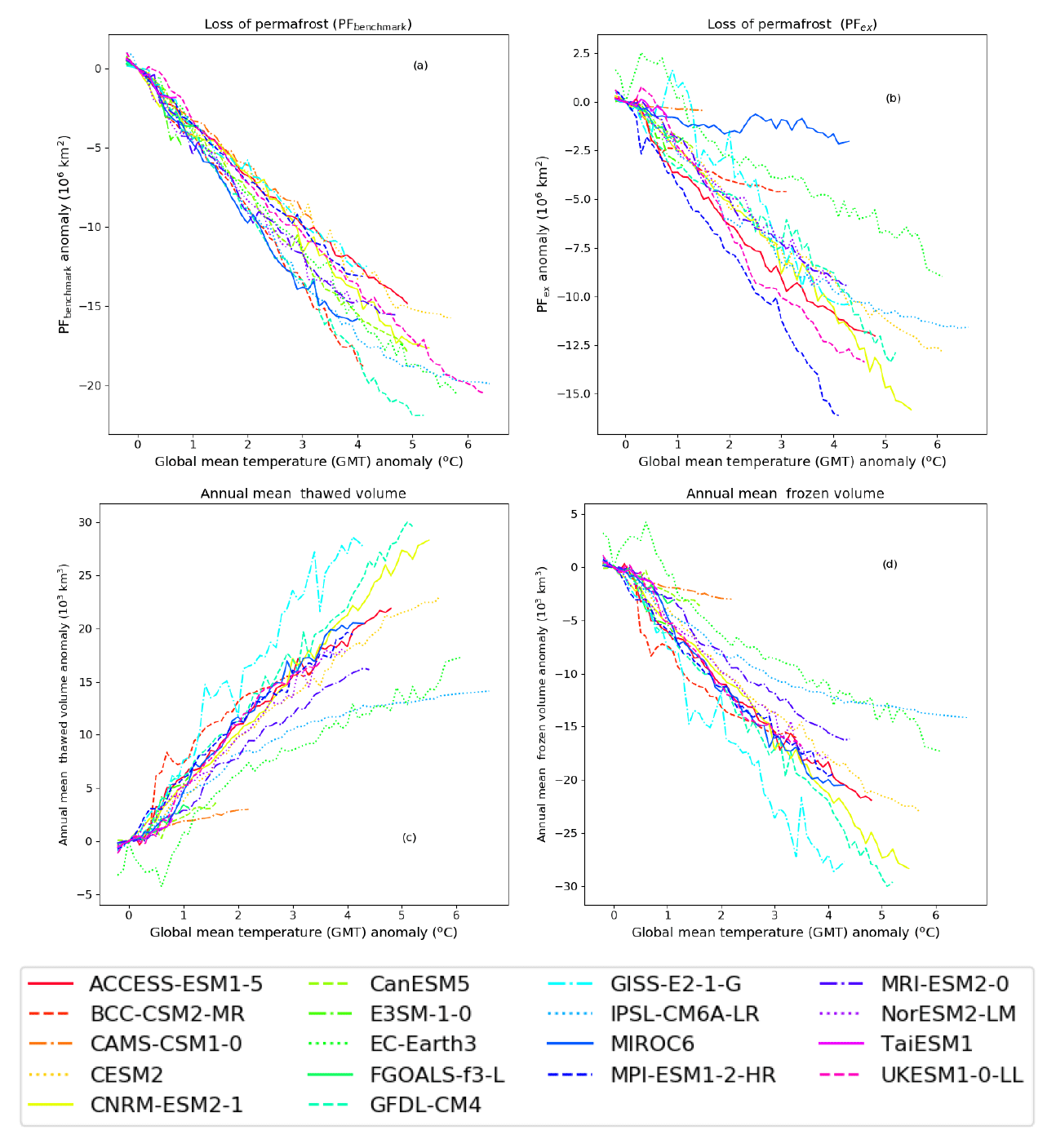
Figure 12 Projections of (a) loss of permafrost extent defined as PF_benchmark derived from the MAAT, (b) loss of permafrost extent defined as PF_ex derived from the soil temperatures, (c) increase in annual mean thawed volume and (d) loss of annual mean frozen volume as a function of global surface air temperature change for the CMIP6 models. All the available scenarios are superimposed on one figure and the results binned into 0.1 ^∘C global surface air temperature change (GSAT) bins. PF_ex is greater than 1×10⁶ km² in all cases.

Table 5 Projections of loss of PF_benchmark, PF_ex and ${\stackrel{\mathrm{̃}}{D}}_{\text{tot}}$ as a function of sensitivity to global surface air temperature change (GSAT). The 50th percentile is shown in bold.

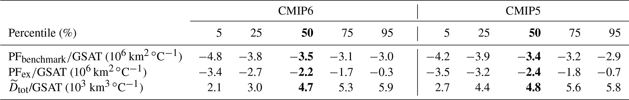
The sensitivity of PF_ex to increasing GSAT is related to both the climate and the land surface module and has a wider range of values from 1.7 to 2.7×10⁶ ${\mathrm{km}}^{\mathrm{2}}{}^{\circ }{\mathrm{C}}^{-\mathrm{1}}$ for the 25th to 75th percentile (Table 5). This range is around 12 % to 20 $\mathrm{\%}{}^{\circ }{\mathrm{C}}^{-\mathrm{1}}$ of the present-day permafrost and is comparable to the CMIP5 sensitivities. The loss of permafrost derived from PF_ex is less than from PF_benchmark. One reason for this is that PF_ex includes the interactions of snow and soil thermal and hydrological dynamics. In addition PF_ex represents a transient response to GSAT. Despite the shallow soil profile in the majority of the models, the methodology used to derive the PF_ex means there will be some implicit time delay in the heat transfer from the surface. There are a few outliers in Fig. 12b which have very different sensitivities of PF_ex to increasing GSAT. These outliers include the MIROC6 model which projects a low sensitivity of PF_ex to GSAT in both the CMIP6 and CMIP5 multi-model ensembles (see also Fig. S2.11). Although there is some improvement in the winter offset in MIROC6 between CMIP5 and CMIP6 (Figs. S2.6 and 7), there is still too little snow insulation in the present-day model because S_depth,eff is relatively shallow. In addition the slope of the relationship between MAGT and MAAT is greater than 1. These factors mean MIROC6 has a “permafrost-prone climate” (Slater and Lawrence, 2013).

The increase in mean thawed volume (${\stackrel{\mathrm{̃}}{D}}_{\text{tot}}$) or the decrease in mean frozen volume (${\stackrel{\mathrm{̃}}{F}}_{\text{tot}}$) is actually relatively consistent between the different models and ranges from 2.1 to 5.9×10³ ${\mathrm{km}}^{\mathrm{3}}{}^{\circ }{\mathrm{C}}^{-\mathrm{1}}$ (5th to 95th percentile; Table 5). This represents a mean loss of frozen volume of around 10 %–40 % of the permafrost in the top 2 m of the soil per degree increase in GSAT (5th to 95th percentile). Here MIROC6 is not an outlier – the sensitivity of ${\stackrel{\mathrm{̃}}{D}}_{\text{tot}}$ and ${\stackrel{\mathrm{̃}}{F}}_{\text{tot}}$ to GSAT in MIROC6 falls within the spread of the other models and the relationship between $\stackrel{\mathrm{̃}}{D}$ and MAGT is comparable with the observed relationship. This suggests that the summer thawing processes are well represented in MIROC6 despite some biases in the sensitivity of the mean deep soil temperature to temperature change. In contrast, the IPSL-CM6A-LR model has a much lower sensitivity of ${\stackrel{\mathrm{̃}}{D}}_{\text{tot}}$ and ${\stackrel{\mathrm{̃}}{F}}_{\text{tot}}$ to GSAT. This is because it does not represent the latent heat required for thawing and therefore has too deep an active layer. However, it falls within the spread of the sensitivity of the PF_ex to GSAT. This is mainly because it has a very deep soil profile and the PF_ex is diagnosed at D_zaa. These examples illustrate how the parameterisation of permafrost physics can affect the projections in different ways.

4 Discussion and conclusion

This paper examines the permafrost dynamics in both the CMIP6 multi-model ensemble and CMIP5 multi-model ensemble using a wide range of metrics. As far as possible, the metrics were defined so as to identify the effect of biases in the climate separately to biases in the land surface module. Overall, the two multi-model ensembles are very similar in terms of climate, snow and permafrost physics and projected changes under future climate change. This paper does not attempt to document specific improvements to individual models in any detail – the CMIP5 and CMIP6 ensembles contains a slightly different set of models. However, it is apparent that the snow insulation is improved in a few of the models which results in overall less variability in the permafrost extent (PF_ex) in the CMIP6 ensemble than in the CMIP5 ensemble. In general, the ability of the models to simulate summer thaw depths is little improved between ensembles. One reason for this remains limitations caused by shallow and poorly resolved soil profiles.

Over the past few years there have been a lot of model developments that have improved the representation of northern high-latitude processes in land surface models (e.g. Chadburn et al., 2015; Porada et al., 2016; Guimberteau et al., 2018; Cuntz and Haverd, 2018; Burke et al., 2017a; Hagemann et al., 2016; Lee et al., 2014). Chadburn et al. (2015) and Porada et al. (2016) developed a dynamic moss parameterisation, which enables the insulation effect of the moss on the permafrost to be simulated. Burke et al. (2017a) added a vertically resolved soil carbon model to enable the permafrost carbon to be identified and traced through the soil. Lee et al. (2014) included a representation of excess ice within the soil which will melt in response to climate change. Many of these processes are yet to be included within the climate models.

In particular, excess ground ice which exists as ice lenses or wedges in permafrost soils is a key process that is not included in the current generation of CMIP models. Thawing of ice-rich permafrost ground will lead to landscape changes including subsidence, thaw slumps and active layer detachments and large-scale modification of the hydrological cycle (Liljedahl et al., 2016; Nitzbon et al., 2020). These ice-rich thermokarst landscapes are susceptible to abrupt changes and cover about 20 % of the northern permafrost region (Olefeldt et al., 2016). Recent observations suggest that even very cold permafrost with near-surface excess ice is highly vulnerable to rapid thermokarst development and degradation (Farquharson et al., 2019). The inclusion of these processes within the CMIP6 models will further perturb the hydrological cycle (e.g. Fraser et al., 2018) and result in additional permafrost degradation not yet quantified by the current generation of climate models.

The CMIP6 models project a loss of permafrost under future climate change of between 1.7 and 2.7×10⁶ ${\mathrm{km}}^{\mathrm{2}}{}^{\circ }{\mathrm{C}}^{-\mathrm{1}}$. A more impact-relevant statistic is the decrease in annual mean frozen volume (3.0 to 5.3×10³ ${\mathrm{km}}^{\mathrm{3}}{}^{\circ }{\mathrm{C}}^{-\mathrm{1}}$) or around 10 %–40 $\mathrm{\%}{}^{\circ }{\mathrm{C}}^{-\mathrm{1}}$. The projections presented here can be used to explore the consequences of permafrost degradation on the large-scale hydrological and carbon cycles, for example, additional sea level rise (Zhang et al., 2000) and the additional loss of permafrost carbon (Turetsky et al., 2020; Burke et al., 2017b).