ISMIP6 Antarctica: a multi-model ensemble of the Antarctic ice sheet evolution over the 21st century

Ice flow models of the Antarctic ice sheet are commonly used to simulate its future evolution in response to different climate scenarios and assess the mass loss that would contribute to future sea level rise. However, there is currently no consensus on estimates of the future mass balance of the ice sheet, primarily because of differences in the representation of physical processes, forcings employed and initial states of ice sheet models. This study presents results from ice flow model simulations from 13 international groups focusing on the evolution of the Antarctic ice sheet during the period 2015–2100 as part of the Ice Sheet Model Intercomparison for CMIP6 (ISMIP6). They are forced with outputs from a subset of models from the Coupled Model Intercomparison Project Phase 5 (CMIP5), representative of the spread in climate model results. Simulations of the Antarctic ice sheet contribution to sea level rise in response to increased warming during this period varies between −7.8 and 30.0 cm of sea level equivalent (SLE) under Representative Concentration Pathway (RCP) 8.5 scenario forcing. These numbers are relative to a control experiment with constant climate conditions and should therefore be added to the mass loss contribution under climate conditions similar to present-day conditions over the same period. The simulated evolution of the West Antarctic ice sheet varies widely among models, with an overall mass loss, up to 18.0 cm SLE, in response to changes in oceanic conditions. East Antarctica mass change varies between −6.1 and 8.3 cm SLE in the simulations, with a significant increase in surface mass balance outweighing the increased ice discharge under most RCP 8.5 scenario forcings. The inclusion of ice shelf collapse, here assumed to be caused by large amounts of liquid water ponding at the surface of ice shelves, yields an additional simulated mass loss of 28 mm compared to simulations without ice shelf collapse. The largest sources of uncertainty come from the climate forcing, the ocean-induced melt rates, the calibration of these melt rates based on oceanic conditions taken outside of ice shelf cavities and the ice sheet dynamic response to these oceanic changes. Results under RCP 2.6 scenario based on two CMIP5 climate models show an additional mass loss of 0 and 3 cm of SLE on average compared to simulations done under present-day conditions for the two CMIP5 forcings used and display limited mass gain in East Antarctica.

1 Introduction

Remote sensing observations of the Antarctic ice sheet have shown continuous ice mass loss over at least the past 4 decades (Rignot et al., 2019; Shepherd et al., 2019, 2018), in response to changes in oceanic (Thomas et al., 2004; Jenkins et al., 2010) and atmospheric (Vaughan and Doake, 1996; Scambos et al., 2000) conditions. This overall mass loss has large spatial variations, as regions around Antarctica experience varying climate change patterns, and individual glaciers respond differently to similar forcings depending on their local geometry and internal dynamics (Durand et al., 2011; Nias et al., 2016; Morlighem et al., 2020). To date, the Amundsen and Bellingshausen sea sectors of West Antarctica and the Antarctic Peninsula have experienced significant mass loss, while East Antarctica has had a limited response to climate change (Paolo et al., 2015; Gardner et al., 2018; Rignot et al., 2019).

Despite the rapid increase in the number of observations (e.g., Rignot et al., 2019; Gardner et al., 2018) and the recent progresses of numerical ice flow models in capturing physical processes (e.g., grounding line migration, ice front evolution) and developing assimilation methods over the past decade (Goelzer et al., 2017; Pattyn et al., 2017), the uncertainty in the Antarctic ice sheet contribution to sea level over the coming centuries remains high (Ritz et al., 2015; DeConto and Pollard, 2016; Edwards et al., 2019). Understanding processes that caused past ice sheet changes and reproducing them is critical in order to improve and gain confidence in projections of ice sheet evolution over the next decades and centuries in response to climate change. Previous modeling studies showed variable Antarctic contribution to sea level rise over the coming century, depending on the physical processes included (e.g., Edwards et al., 2019), model initial states (e.g., Seroussi et al., 2019; Goelzer et al., 2018), forcing used (e.g., Golledge et al., 2015; Schlegel et al., 2018) or model parameterizations (e.g., Bulthuis et al., 2019), leading to results varying between a few millimeters to more than a meter of sea level contribution by the end of the century (Ritz et al., 2015; Pollard et al., 2015; Little et al., 2013; Levermann et al., 2014). Model intercomparison efforts such as Ice2Sea (Edwards et al., 2014) and SeaRISE (Sea-level Response to Ice Sheet Evolution, Bindschadler et al., 2013; Nowicki et al., 2013a) highlighted the large discrepancies in numerical ice flow model results, even when similar climate conditions are applied for model forcing. Furthermore, most of these experiments were carried out under extremely simplified climate forcings, limiting our understanding of how ice sheets may respond to realistic climate scenarios.

ISMIP6 (Ice Sheet Model Intercomparison Project for CMIP6, Nowicki et al., 2016) is the primary effort of CMIP6 (Climate Model Intercomparison Project Phase 6) focusing on ice sheets and was designed to address these questions and improve our understanding of ice sheet–climate interactions. In a first stage, ice sheet model initialization experiments (initMIP, Goelzer et al., 2018; Seroussi et al., 2019) focused on the role of initial conditions and model parameters in ice flow simulations. Antarctic experiments were based on simplified forcings: the surface mass balance (SMB) was averaged between several global and regional climate models and the ocean-induced basal melt was doubled compared to the amount of basal melt estimated from remote sensing observations (Depoorter et al., 2013; Rignot et al., 2013). These experiments were used to assess the response of ice flow models to anomalies in these external forcings (Seroussi et al., 2019). Results showed that models respond similarly to changes in SMB, while changes in ocean-induced basal melt cause a large spread in model response. The initial ice shelf extent, which varies by a factor of 2.5 between the models with the smallest and largest ice shelf extents, as well as the treatment of sub-ice-shelf basal melt close to the grounding line and the model spatial resolution, were identified as the main sources of differences between the simulations (Seroussi et al., 2019).

In this study, we focus on projections of the Antarctic ice sheet forced by outputs from CMIP5 Atmosphere–Ocean General Circulation Models (AOGCMs), including both Climate Models and Earth System Models, under different climate conditions, as CMIP6 results were not available when the experimental protocol was designed (Nowicki et al., 2020). The ensemble of simulations focuses mostly on the 2015–2100 period and is based on 21 sets of ice flow simulations submitted by 13 international institutions. We investigate the relative role of climate forcings, Representative Concentration Pathway (RCP) scenarios, ocean-induced melt parameterizations and simulated physical processes on the Antarctic ice sheet contribution to sea level and the associated uncertainties. Most of the results are presented relative to simulations with a constant climate and therefore show the impact of climate warming relative to a scenario with a constant climate. We first describe the experiment setup and the forcings used for the simulations in Sect. 2. We then detail the ice flow models that took part in this intercomparison and summarize their main characteristics in Sect. 3. Section 4 analyzes the results and assesses the impact of the different scenarios and processes explored. Finally, we discuss the results, differences between models, most vulnerable regions and the main sources of uncertainties in Sect. 5.

2 Climate forcings and experiments

ISMIP6 is an endorsed MIP (Model Intercomparison Project) of CMIP6, and experiments performed as part of ISMIP6 projections are therefore based on outputs from AOGCMs taking part in CMIP. As results from CMIP6 were not available at the time the experimental protocol was determined (Nowicki et al., 2020), it was decided to rely primarily on available CMIP5 outputs to assess the future evolution of the Greenland (Goelzer et al., 2020) and Antarctic ice sheets. This choice allowed an in-depth analysis of CMIP5 AOGCM outputs and the selection of a subset of CMIP5 models that would capture the spread of climate evolution. The choice of using only a subset of AOGCMs limits the number of simulations required from each ice sheet modeling group, while still sampling the uncertainty in future ice sheet evolution associated with variations in climate models (Barthel et al., 2020). Additional simulations based on CMIP6 are ongoing and will be the subject of a forthcoming publication.

In this section, we summarize the experimental protocol for ISMIP6-Antarctica projections, including the choice of CMIP5 climate and Earth system models, the processing of their outputs in order to derive atmospheric and oceanic forcings applicable to ice sheet models, and the processes included in the experiments. We then list the experiments analyzed in the present work. More details on the experimental protocol can be found in Nowicki et al. (2020), while the selection of the CMIP5 model ensemble is explained in Barthel et al. (2020). A detailed description of the ocean melt parameterization and calibration is available in Jourdain et al. (2020).

2.1 Selection of CMIP5 climate models

The forcings applied to ISMIP6-Antarctica projections are derived from both RCP 8.5 and RCP 2.6 scenarios, with most experiments based on RCP 8.5, in order to estimate the full extent of changes possible by 2100 with varying climate forcings. A few RCP 2.6 scenarios are used to assess the response of the ice sheet to more moderate climate changes.

After selecting CMIP5 climate and Earth system models that performed both RCP 8.5 and RCP 2.6 scenarios, they were first assessed on their ability to represent present climate conditions around the Antarctic ice sheet. A historical bias metric was computed, incorporating atmosphere and surface oceanic conditions south of 40^∘ S and oceanic conditions in six ocean sectors shallower than 1500 m around Antarctica. Atmospheric and surface metrics were evaluated against the European Centre for Medium-Range Weather Forecasts “Interim” reanalysis (ERA-Interim, Dee et al., 2011). Ocean metrics were compared to a reference climatology combining the 2018 World Ocean Atlas (Locarnini et al., 2019), EN4 ocean climatology (Good et al., 2013) and temperature profiles from Logger-equipped seals (Roquet et al., 2018). Following this assessment of AOGCMs, we analyzed the changes projected between 1980–2000 and 2080–2100 in oceanic and atmospheric conditions under the RCP 8.5 scenario. We chose six CMIP5 models that performed better than the median at capturing present-day conditions and represented a large diversity in projected changes. These climate and Earth system models are CCSM4, MIROC-ESM-CHEM, and NorESM1-M for the core experiments and CSIRO-Mk3-6-0, HadGEM2-ES, and IPSL-CM5A-M for the CMIP5 Tier 2 experiments (see Sect. 2.5). Two of these models, NorESM1-M and IPSL-CM5A-M, were also chosen to provide forcings for the RCP 2.6 scenario. We refer to Barthel et al. (2020) for a detailed description of the model evaluation and selection.

This choice of CMIP5 models was designed both to select models that best capture the variables relevant to ice sheet evolution and to maximize the diversity in projected 21st century climate evolution, while limiting the number of simulations. CMIP5 model choices were made independently for Greenland and Antarctica, to focus on the specificities of each ice sheet and region. We derived external forcings for the Antarctic ice sheet from these CMIP5 model outputs and provided yearly forcing anomalies for participating models.

2.2 Atmospheric forcing

Using the CMIP5 models selected, atmospheric forcings were derived in the form of yearly averaged surface mass balance anomalies and surface temperature anomalies compared to the 1980–2000 period. The SMB anomalies include changes in precipitation, evaporation, sublimation and runoff and are presented in the form of water-equivalent quantities. These anomalies are then added to reference surface mass balance and surface temperature fields that are used as a baseline in the ice flow models, similar to the approach used in Seroussi et al. (2019).

SMB conditions are often estimated using Regional Climate Models (RCMs), such as the Regional Atmospheric Climate Model (RACMO, Lenaerts et al., 2012; van Wessem et al., 2018) and Modèle Atmosphérique Régional (MAR, Agosta et al., 2019), forced at their boundaries with AOGCMs outputs. As high-resolution RCM integrations for the full Antarctic ice sheet are complex and typically require additional boundary forcing and considerable time and computational resources, it was decided not to follow this approach for ISMIP6-Antarctica Projections but to use AOGCM outputs directly. Further details on the derivation of atmospheric forcing can be found in Nowicki et al. (2020).

2.3 Oceanic forcing

Melting at the base of ice shelves is caused by the underlying circulation of ocean waters, with warmer waters and stronger currents increasing the amount of basal melt. However, converting ocean properties into basal melt forcing under the ice shelves remains challenging (Favier et al., 2019). Similar to what is done for the atmospheric forcing, the ocean forcing is derived from the CMIP5 AOGCMs outputs. However, the CMIP5 models do not always resolve the Antarctic continental shelf, and none include ice shelf cavities. The first task to prepare the ocean forcing was therefore to extrapolate relevant oceanic conditions (temperature and salinity) to areas not included in CMIP5 ocean models, including areas currently covered by ice that could become ice-free in the future. These areas include sub-ice-shelf cavities and areas beneath the grounded ice sheet that could be exposed to the ocean following ice thinning and grounding line retreat. Three-dimensional fields of ocean salinity, temperature and thermal forcing were then computed as annual mean values over the 1995–2100 period. We refer to Jourdain et al. (2020) for more details on the extrapolation of oceanic fields and computation of ocean thermal forcing.

Converting ocean conditions into ocean-induced melt at the base of ice shelves is an active area of research, and several parameterizations with different levels of complexity have recently been proposed for converting ocean conditions into ice shelf melt rates (e.g., Lazeroms et al., 2018; Reese et al., 2018a; Pelle et al., 2019). As only a limited number of direct observations of ocean conditions (e.g., Jenkins et al., 2010; Dutrieux et al., 2014) and ice shelf melt rates (e.g., Rignot et al., 2013; Depoorter et al., 2013) exist, these parameterizations are difficult to calibrate and evaluate. Some parameterizations are relatively complex and based on nonlocal quantities and can therefore be difficult to implement in continental-scale parallel ice sheet models. Furthermore, such parameterizations do not account for feedbacks between the ice and ocean dynamics, which are likely only captured by coupled ice–ocean models (De Rydt and Gudmundsson, 2016; Seroussi et al., 2017; Favier et al., 2019).

For these reasons, ISMIP6-Antarctica Projections includes two options that can be adopted for the sub-ice-shelf melt parameterization: (1) a standard parameterization based on a prescribed relation between ocean thermal forcing and ice shelf melting rates and (2) an open parameterization left to the discretion of the ice sheet modeling groups. Such a framework allows us to evaluate the response to a wide spectrum of melt parameterizations with the open framework while also capturing the uncertainty related to the ice sheet response under a more constrained setup in the standard framework. The standard parameterization was chosen as a trade-off between a simple parameterization that most modeling groups could implement in a limited time while capturing melt rate patterns as realistically as possible. Results from an idealized case comparing coupled ice–ocean models with different melt parameterizations suggested that a nonlocal, quadratic melt parameterization was best able to mimic the coupled ice–ocean results over a broad range of ocean forcing (Favier et al., 2019). These results were performed on an idealized case similar to the Marine Ice Sheet Ocean Model Intercomparison Project (MISOMIP, Asay-Davis et al., 2016; Cornford et al., 2020) and have not yet been tested on realistic geometries. The non-quadratic melt parameterization suggested in Favier et al. (2019) is as follows:

$$\begin{array}{}\text{(1)}& \begin{array}{rl}m\left(x,y\right)& ={\mathit{\gamma }}_{\mathrm{0}}\times {\left({\displaystyle \frac{{\mathit{\rho }}_{\mathrm{sw}}{c}_{\mathrm{pw}}}{{\mathit{\rho }}_{\mathrm{i}}{L}_{\mathrm{f}}}}\right)}^{\mathrm{2}}\times \left(\mathrm{TF}\left(x,y,z_{\text{draft}}\right)\right.\\ & \left.+\mathit{\delta }{T}_{\text{sector}}\right)\times \left|\langle \mathrm{TF}{\rangle }_{\text{draft}\in \text{sector}}+\mathit{\delta }{T}_{\text{sector}}\right|,\end{array}\end{array}$$

where γ₀ is a coefficient similar to an exchange velocity, ρ_sw the ocean density, c_pw the specific heat of sea water, ρ_i the ice density, L_f the ice latent heat of fusion, TF $(x,y,z_{\text{draft}})$ the local ocean thermal forcing at the ice shelf base, |〈TF〉_{draft∈sector}| the ocean thermal forcing averaged over a sector and δT_sector the temperature correction for each sector. The values for γ₀ and δT_sector in this equation were calibrated combining observations of ocean conditions (Locarnini et al., 2019; Good et al., 2013) and remote sensing estimates of melt rates (Rignot et al., 2013; Depoorter et al., 2013). Two calibrations based either on circum-Antarctic observations (the “MeanAnt” method) or on observations close to the grounding line of Pine Island Glacier (the “PIGL” method) were performed in a two-step process. The coefficient γ₀ is first calibrated assuming δT equal to zero and using 10⁵ random samplings of melt rate and ocean temperature, so that the total melt produced under the ice shelves is similar to melt rates estimated in Rignot et al. (2013) and Depoorter et al. (2013). This process provides a distribution of possible γ₀ values. The δT_sector values are then calibrated for each of the 16 sectors of Antarctica (see Jourdain et al., 2020, for details), so that the melt in each basin agrees with average estimated melt in this sector. The median value of γ₀ is used for all but two runs. These two experiments assess the impact of uncertainty in γ₀ by using the 5th and 95th percentile values from the distribution. The second calibration, “PIGL”, uses the same process but is constrained with only a subset of observations under Pine Island ice shelf and close to its grounding line, since these values are the most relevant for highly dynamic ice streams that have the highest sub-shelf melt (Reese et al., 2018b). This calibration leads to higher values of γ₀, corresponding to a greater sensitivity of melt rates to changes in ocean temperature.

The choice of melt parameterization and its calibration with observations is described in detail in Jourdain et al. (2020). For models that could not implement such a nonlocal parameterization, a local quadratic parameterization similar to Eq. (1), with the nonlocal thermal forcing replaced by local thermal forcing, was also designed and calibrated to provide similar results (Jourdain et al., 2020).

2.4 Ice shelf collapse forcing

Several ice shelves in the Antarctic Peninsula have collapsed over the past 3 decades (Doake and Vaughan, 1991; Scambos et al., 2004, 2009). One mechanism proposed to explain the collapse of these ice shelves is the presence of significant amounts of liquid water on their surface, which causes hydrofracturing and ultimately leads to their collapse (Vaughan and Doake, 1996; Banwell et al., 2013; Robel et al., 2019). Other mechanisms, such as ocean surface waves, rheological weakening, surface load shifts due to water movement or basal melting (MacAyeal et al., 2003; Braun and Humbert, 2009; Borstad et al., 2012; Banwell et al., 2013; Banwell and Macayeal, 2015), have also been proposed to explain these ice shelf collapse but are not investigated in this study. Ice shelf collapse reduces the buttressing forces provided to the upstream grounded ice and leads to acceleration and increased mass loss of the glaciers feeding them (De Angelis and Skvarca, 2003; Rignot et al., 2004), but more dramatic consequences have been envisioned if ice shelves were to collapse in front of thick glaciers resting on retrograde bed slopes (Bassis and Walker, 2011; DeConto and Pollard, 2016). As the presence of liquid water at the surface of Antarctic ice shelves is expected to increase in a warming climate (Mercer, 1978; Trusel et al., 2015), we propose experiments that include ice shelf collapse. The response of grounded ice streams to such a collapse is not imposed but arises from the various model representations of boundary conditions and transitions from grounded to floating ice. Apart from these experiments testing the impact of ice shelf collapse, the other experiments should not include ice shelf collapse.

Ice shelf collapse forcing is described as a yearly mask that defines the regions and times of collapse. The criteria for ice shelf collapse are based on the presence of mean annual surface melting above 725 mm over a decade, similar to numbers proposed in Trusel et al. (2015), and corresponding to the average melt simulated by RACMO2 over the Larsen A and B ice shelves in the decade before their collapse. The amount of surface melting was computed from CMIP5 modeled surface air temperature using the methodology described in Trusel et al. (2015).

2.5 List of experiments

The list of experiments for ISMIP6-Antarctica Projections is described and detailed in Nowicki et al. (2020). It includes a historical experiment (historical), control runs (ctrl and ctrl_proj), simple anomaly experiments similar to initMIP-Antarctica (asmb and abmb), 13 core (Tier 1) experiments, and 8 Tier 2 experiments based on CMIP5 forcing. The list is repeated in Table 1 for completeness. In summary, these experiments include the following variations:

• 12 experiments based on RCP 8.5 scenarios from 6 CMIP5 models (open and standard melt parameterizations);

• 4 experiments based on RCP 2.6 scenarios from 2 CMIP5 models (open and standard melt parameterizations);

• 2 experiments including ice shelf collapse (open and standard melt parameterizations);

• 2 experiments testing the uncertainty in the melt parameterization (standard melt parameterization only);

• 2 experiments testing the uncertainty in the melt calibration (standard melt parameterizations only).

All experiments start in 2015, except for the historical, ctrl, asmb and abmb experiments, which start at the model initialization time. The historical experiment runs from the initialization time until the beginning of 2015, while the ctrl, asmb and abmb experiments run for either 100 years or until 2100, whichever is longer. All the other experiments run from January 2015 to the end of 2100. The ctrl_proj run is a control run similar to ctrl: a simulation under constant climate conditions representative of the recent past. The only difference is that ctrl_proj starts in 2015 and lasts until 2100, while ctrl starts from the ice models' initial state (which varies between 1850 and 2015 for the various models) and lasts at least 100 years.

Table 1 List of ISMIP6-Antarctica projections for the core (Tier 1) and Tier 2 experiments based on CMIP5 AOGCMs.

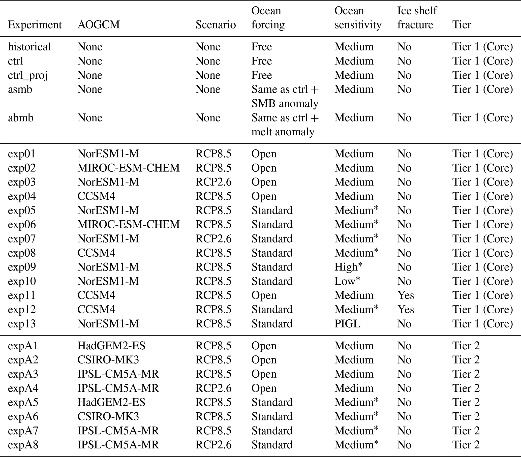
^∗ For the “standard” parameterization, the low, medium and high ocean sensitivity correspond to the 5th, 50th and 95th percentile values of the “MeantAnt” γ₀ distribution (Jourdain et al., 2020).

Most analyses presented in this study follow an “experiment minus ctrl_proj” approach, so the results provide the impact of change in climatic conditions relative to ice sheets forced with present-day conditions until 2100. We know that ice sheets respond nonlinearly to changes in climate conditions, but such an approach is necessary as ice flow model simulations often do not accurately capture the trends observed over the recent past (Seroussi et al., 2019).

3 Ice flow models

3.1 Model setups

Similar to the philosophy adopted for initMIP-Antarctica, there are no constraints on the method or datasets used to initialize ice sheet models. The exact initialization date is also left to the discretion of individual modeling groups, thus the historical experiment length varies among groups (some groups start directly at the beginning of 2015 and therefore did not submit a historical run). The resulting ensemble includes a variety of model resolutions, stress balance approximations and initialization methods, representative of the diversity of the ice sheet modeling community (see Sect. 3.2 for more details on participating models).

The only constraints imposed on the ice sheet models are that (1) models have to simulate ice shelves and the evolution of grounding lines and that (2) models have to use the atmospheric and oceanic forcings varying in time and based on CMIP5 model outputs provided. The inclusion of ice cliff failure, on the other hand, was not allowed, except in the ice shelf collapse experiments. Groups were invited to submit one or several sets of experiments, and modelers were asked to submit the full suite of open (with the melt parameterization of their choice; see Table 3) and/or standard (Jourdain et al., 2020) core experiments if possible. Unlike what was imposed for initMIP-Antarctica, models were free to include additional processes not specified here (e.g., changes in bedrock topography in response to changes in ice load, feedback between SMB and surface elevation).

Annual values for both scalar and two-dimensional outputs were reported on standard grids with resolutions of 4, 8, 16 or 32 km. Scalar quantities were recomputed from the two-dimensional fields submitted for consistency and in order to create regional scalars used for the regional analysis. The two-dimensional fields were also conservatively regridded onto the standard 8 km grid to facilitate spatial comparison and analysis. The outputs requested are listed in Appendix A. Each group also submitted a README file summarizing the model characteristics.

3.2 Participating models

A total of 16 sets of simulations from 13 groups were submitted to ISMIP6-Antarctica projections. The groups and ice sheet modelers who ran the simulations are listed in Table 2. Simulations are performed using various ice flow models, a range of grid resolutions, different approximations of the stress balance equation, varying basal sliding laws, and multiple external forcings; a diverse set of processes were included in the simulations. Table 3 summarizes the main characteristics of the 16 sets of simulations. Short descriptions of the initialization method and main model characteristics are also provided in Appendix C.

Table 2 List of participants, modeling groups and ice flow models in ISMIP6-Antarctica projections.

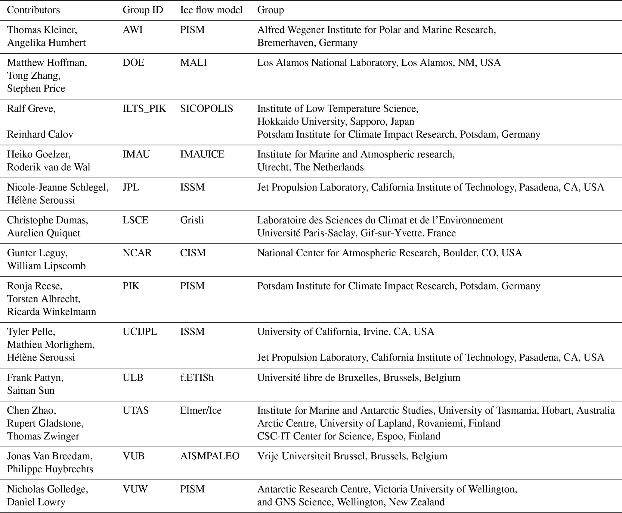
Table 3 List of ISMIP6-Antarctica projection simulations and main model characteristics. Numerics are defined as follows: finite difference (FD), finite elements (FE) and finite volumes (FV). Initialization methods used are as follows: spin-up (SP), spin-up with ice thickness target values (SP+; see Pollard and DeConto, 2012a), data assimilation (DA), data assimilation with relaxation (DA+), data assimilation of ice geometry only (DA^∗) and equilibrium state (Eq). Melt in partially floating cells is listed as follows: melt either applied or not applied over the entire cell based on a floating condition (floating condition) and melt applied based on a sub-grid scheme (sub-grid); N/A refers to models that do not have partially floating cells. Ice front migration schemes are based on strain rate (StR, Albrecht and Levermann, 2012), retreat only (RO), fixed front (fix), minimum thickness height (MH), and divergence and accumulated damage (div, Pollard et al., 2015). Basal melt rate parameterization in open framework are listed as follows: linear function of thermal forcing (lin, Martin et al., 2011), quadratic local function of thermal forcing (quad, DeConto and Pollard, 2016), PICO parameterization (PICO, Reese et al., 2018a), PICOP parameterization (PICOP, Pelle et al., 2019), plume model (Plume, Lazeroms et al., 2018) and nonlocal parameterization with slope dependence of the melt (Nonl4ocal + Slope, Lipscomb et al., 2020). Basal melt rate parameterization in standard framework is listed as follows: local or nonlocal quadratic function of thermal forcing and local or nonlocal anomalies (Jourdain et al., 2020).

The 16 sets of submitted simulations have been performed using 10 different ice flow models. Amongst the simulations, 3 use the finite-element method, 2 use a combination of finite element and finite volume, and the remaining 11 the finite-difference method. One simulation is based on a Full-Stokes stress balance, two use the 3D higher-order approximations (HO, Pattyn, 2003), one is based on the L1L2 approximation (Hindmarsh, 2004) and one is based on the shelfy-stream approximation (SSA, MacAyeal, 1989), while the other simulations combine the SSA with the shallow ice approximation (SIA, Hutter, 1982). The model resolutions range between 4 and 20 km for models that use regular grids but can be as low as 2 km in specific areas, such as close to the grounding line or shear margins for models with spatially variable resolution (Morlighem et al., 2010).

As in initMIP-Antarctica (Seroussi et al., 2019), the initialization procedure reflects the broad diversity in the ice sheet modeling community: two simulations start from an equilibrium state, five models start from a long spin-up and three simulations from data assimilation of recent observations. The remaining simulations combine the latter two approaches by either adding constraints to their spin-up (three simulations) or running short relaxations after performing data assimilation (three simulations). The initialization year varies between 1850 and 2015, therefore the length of the historical experiment varies between 0 and 115 years.

All submissions are required to include grounding line evolution (see Sect. 3.1), but the treatment of grounding line evolution and ocean melt in partially floating grid cells is left to the discretion of the modeling groups. Simulating ice front evolution (i.e., calving) in the simulations is also encouraged but not required, and the choice of ice front parameterization is free. Six models use a fixed ice front (except for the ice shelf collapse experiments, for which retreat is imposed), while the other models rely on a combination of minimum ice thickness, strain rate values and stress divergence to evolve their ice front position.

The simulations were performed using the open and/or standard melt parameterizations: five sets of simulations include results based on both the open and standard framework, leading to a total of 21 sets of simulations in total when the open and standard parameterizations are analyzed separately; this parameterization affects the results significantly, therefore the open and standard parameterizations are analyzed separately from now on. Ocean-induced melt rates under ice shelves follow the standard melt framework described in Sect. 2.3 for 13 sets of simulations: 10 submissions use the nonlocal form, while 3 are based on the local form, and three of these 13 sets of simulations are based on the nonlocal or local anomaly forms (Jourdain et al., 2020). The open melt framework was used by eight sets of simulations that rely on a linear melt dependence of thermal forcing (Martin et al., 2011), a quadratic local melt parameterization (DeConto and Pollard, 2016) with a calibration different than the standard framework, a plume model (Lazeroms et al., 2018), a box model (Reese et al., 2018a), a combination of box and plume models (Pelle et al., 2019), or a nonlocal quadratic melt parameterization combined with ice shelf basal slope (Lipscomb et al., 2020).

The modeling groups were asked to submit a full suite of core experiments based on the standard melt parameterization, the open one or both. Most groups were able to do so, but several groups did not submit the ice shelf collapse experiments, and one group (UTAS_ElmerIce) ran only a subset of experiments due to the high cost of running a Full-Stokes model of the Antarctic continent. Simulations that initialize their model in January 2015 (see Table 3) do not have a historical run, and their ctrl and ctrl_proj are therefore identical. Seven submissions also performed some or all of the Tier 2 experiments (expA1–A8). Table 4 lists all the experiments done by the modeling groups.

Table 4 List of experiments performed as part of ISMIP6-Antarctica projections by the modeling groups.

^∗ Indicates simulations initialized directly at the beginning of 2015 for which ctrl and ctrl_proj experiments are identical.

4 Results

We detail the simulation results here. We start by describing the initial state and the historical and control runs. We then analyze the NorESM1-M RCP 8.5 runs, and the RCP 8.5 simulations based on the six different CMIP5 model forcings. Next, we compare the RCP 8.5 and RCP 2.6 results for the two CMIP5 models selected to provide RCP 2.6 scenario forcings. We then investigate the effect of uncertainty in the melt parameterization and calibration. Finally, we explore the role of ice shelf collapse.

Results based on the open and standard melt parameterizations are combined, except in Sect. 4.6, where we investigate the difference between these approaches. This means that 21 independent sets of results are extracted from the 16 submissions (8 based on the open melt framework and 13 based on the standard framework). No weighting based on the number of submissions or agreement with observations is applied.

4.1 Historical run and 2015 conditions

As the initialization date for different models varies, all models run a short historical simulation until 2015. The length of this simulation varies between 165 years for PIK_PISM1, which starts in 1850, and 0 years for the three models (DOE_MALI, PIK_PISM2 and UTAS_ElmerIce) that start directly in 2015. During the historical run, simulations are forced with oceanic and atmospheric conditions representative of the conditions estimated during this period. The total annual SMB over Antarctica varies between 2140 and 3230 Gt yr⁻¹, with large interannual variations of up to 600 Gt yr⁻¹ (see Fig. 1a). The total annual ocean-induced basal melt rates under ice shelves during the historical period varies between 0 and 4200 Gt yr⁻¹, with large interannual variations up to 500 Gt yr⁻¹. The ice volume above floatation, however, experiences limited variations during the historical period, up to a 6000 Gt change (Fig. 1b).

Figure 1 Evolution of surface mass balance (a, in Gt yr⁻¹), basal melt rate (b, in Gt yr⁻¹) and volume above floatation (c, in Gt) during the historical and ctrl_proj experiments for all the simulations performed with the open and standard framework. Note the different scale on the time axis prior to 1950.

All historical simulations end in December 2014, at which point the projection experiments start. Figure 2 shows the total ice and floating ice extent for all submissions at the beginning of the experiments. The simulated ice-covered area varies between 1.36 and 1.45×10⁷ km², or 6.0 %. There is good agreement between the modeled ice extent and the observed ice front (Howat et al., 2019) around the entire continent and a smaller spread compared to the initMIP-Antarctica submissions, in which the ice extent varied between 1.35 and 1.50×10⁷. The extent of ice shelves shown in Fig. 2b varies between 1.19 and 1.92×10⁶ km², which is a much smaller spread in the results than in the initMIP-Antarctica experiments (between 0.92 and 2.51×10⁶) and a better agreement with observations (Rignot et al., 2011). Not only the large ice shelves but also the smaller ice shelves of the Amundsen and Bellingshausen sea sectors, the Antarctic Peninsula, and Dronning Maud Land have a location and extent that is usually within several tens of kilometers of observations. A few models have ice shelves that extend slightly farther than the present-day ice over large parts of the continent, but they extend only a few tens of kilometers past the observed ice front location. Finally, the location of the grounding line on the Ross ice streams fluctuates by several hundred kilometers between the models, which is not surprising as the Ross ice streams rest over relatively flat bedrock, and thus small changes in model configuration lead to large variations in the grounding line position. The 2015 ice volume and ice volume above floatation are reported in Table B1 and on Fig. 1c. They indicate a variation of 6.8 % of the total ice mass among the simulations, between 2.31 and 2.49×10⁷ Gt, and a variation of 7.7 % in the total ice mass above floatation, between 1.99 and 2.15×10⁷ Gt or between 55.0 and 59.4 m of sea level equivalent (SLE), when the latest estimate is 57.9±0.9 m (Morlighem et al., 2020). Figure 3 shows the root-mean-square error (RMSE) between modeled and observed thickness and velocity at the beginning of the experiments. The RMSE thickness varies between 92 and 396 m, while the RMSE velocity varies between 79 and 446 m yr⁻¹, which is comparable to values reported for initMIP-Antarctica (Seroussi et al., 2019).

4.2 Control experiment ctrl_proj

All the experiments start from the 2015 configuration and are run with varying atmospheric and oceanic forcings until 2100. The ctrl_proj experiment also starts from this configuration but is run with constant climate conditions (no oceanic or atmospheric anomalies added), similar to those observed over the past several decades. The exact choice of forcing conditions for this run was not imposed and therefore varies between the simulations. Figure 1 shows that, similarly to the historical run, the SMB and basal melt vary significantly between the simulations. The SMB varies between 2320 and 3090 Gt yr⁻¹, while the basal melt varies between 0 and 3740 Gt yr⁻¹. However, unlike what is observed in the historical run, there is limited interannual fluctuation, since a mean climatology is used for this run.

During the 86 years of the ctrl_proj experiment, the simulated evolution of ice mass above floatation varies between −51 500 and 46 700 Gt (between −130 and 142 mm SLE; see Table B2). The trend in the ctrl_proj mass above floatation is significant in several models and negligible in others. As in initMIP-Antarctica, models initialized with a steady state or a spin-up tend to have smaller trends than models initialized with data assimilation. Since constant climate conditions are applied, trends cannot be considered a physical response of the Antarctic ice sheet but rather highlight the effect of model choices to initialize the simulation and represent ice sheet evolution, the lack of physical processes (Pattyn, 2017), the limited number or inaccuracy of observations (Seroussi et al., 2011; Gillet-Chaulet et al., 2012), and the need to better integrate observations in ice flow models (Goldberg et al., 2015; Nowicki and Seroussi, 2018).

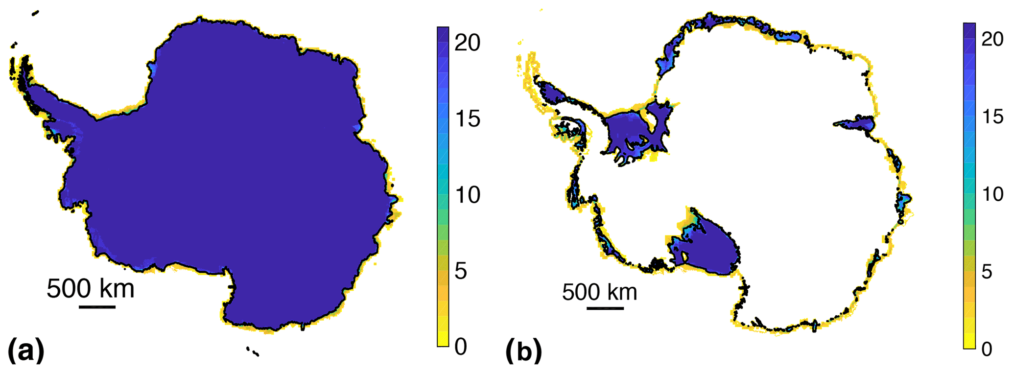
Figure 2 Total (a) and floating (b) ice extent at the beginning of the experiments (January 2015). Colors indicate the number of models simulating total ice (a) and floating ice (b) extent at every point of the 8 km grid. Black lines are observations of the total and floating ice extent, respectively (Morlighem et al., 2020).

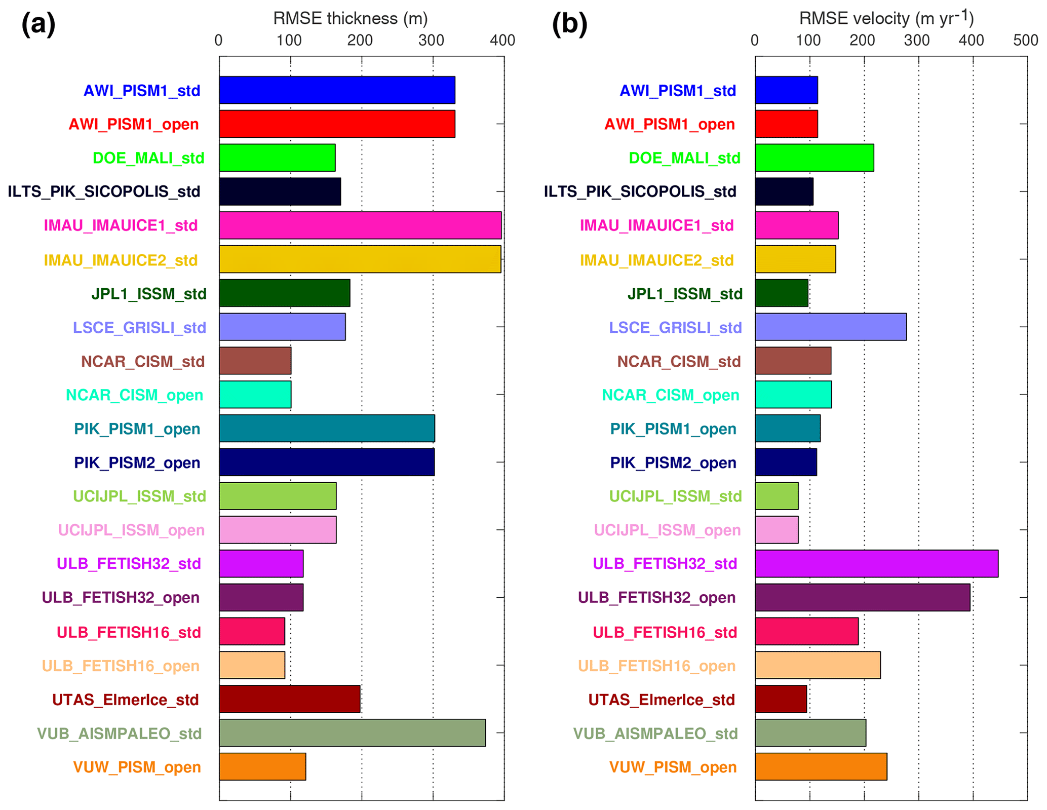
Figure 3 Root-mean-square error in ice thickness (a, in m) and ice velocity (b, in m yr⁻¹) between modeled and observed values at the beginning of the experiments (January 2015).

All the results presented in the remainder of the paper are shown relative to the outputs from the ctrl_proj experiment. As a consequence, these results should be interpreted as the models' simulated response to additional climate change compared to a scenario where the climate remains constant and similar to the past few decades. Submissions that include both open and standard experiment results can have significant variations in their historical and ctrl_proj depending on whether the open or standard melt parameterization is used (see Fig. 1 and Tables B1 and B2). We therefore remove the trends from the ctrl_proj open or standard melt parameterization from the experiments based on the open or standard framework, respectively.

4.3 Projections under RCP 8.5 scenario with NorESM1 forcing

The NorESM1-M RCP 8.5 scenario (exp01 and exp05; see Table 1) produces mid-to-high changes in the ocean and low changes in the atmosphere over the 21st century compared to other CMIP5 AOGCMs (Barthel et al., 2020). The effects of these changes on the simulated evolution of the Antarctic ice sheet are summarized in Figs. 4, 5 and 6. Figure 4 shows that under this forcing, the ice sheet loses a volume above floatation varying between −26 and 166 mm of SLE between 2015 and 2100, relative to ctrl_proj experiments. The impact of the forcing remains limited until 2050, with changes between −2 and 27 mm. It quickly increases after 2050, at which point the simulations start to diverge strongly.

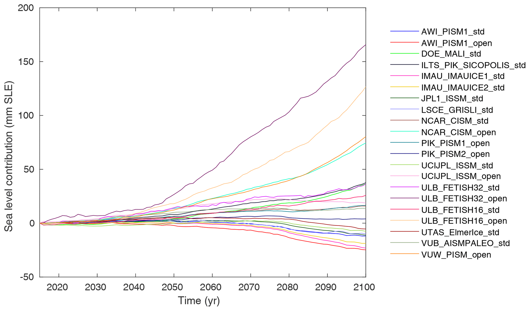
Figure 4 Evolution of ice volume above floatation (in mm SLE) over 2015–2100 from the NorESM1-M RCP 8.5 scenario (exp01 and exp05) relative to ctrl_proj.

Figure 5 shows that the sea level contribution and the mechanisms at play vary significantly for the West Antarctic ice sheet (WAIS), East Antarctic ice sheet (EAIS) and the Antarctic Peninsula. In the WAIS, the additional SMB is limited to a few millimeters (between −2 and 2 mm SLE), and all models predict a mass loss varying between 0 and 154 mm SLE relative to ctrl_proj. EAIS experiences a significant increase in SMB, with a cumulative additional SMB causing between 20 and 25 mm SLE of mass gain relative to ctrl_proj. This mass gain is partially offset by the dynamic response of outlet glaciers in the EAIS, resulting in a total volume change varying between a 24 mm SLE mass gain and 38 mm SLE mass loss. The small size of the Antarctic Peninsula and limited mass of its glaciers make it a smaller contributor to sea level change compared to WAIS and EAIS: the contribution to sea level varies between −6 and 1 mm SLE relative to ctrl_proj, with a signal split between the additional SMB (between 0 and 3 mm SLE mass gain) and dynamic response. These results therefore highlight the contrast between the EAIS and the Antarctic Peninsula, which are projected to either gain or lose mass and where SMB changes are relatively large, and the WAIS, which is dominated by a dynamic mass loss caused by the changing ocean conditions.

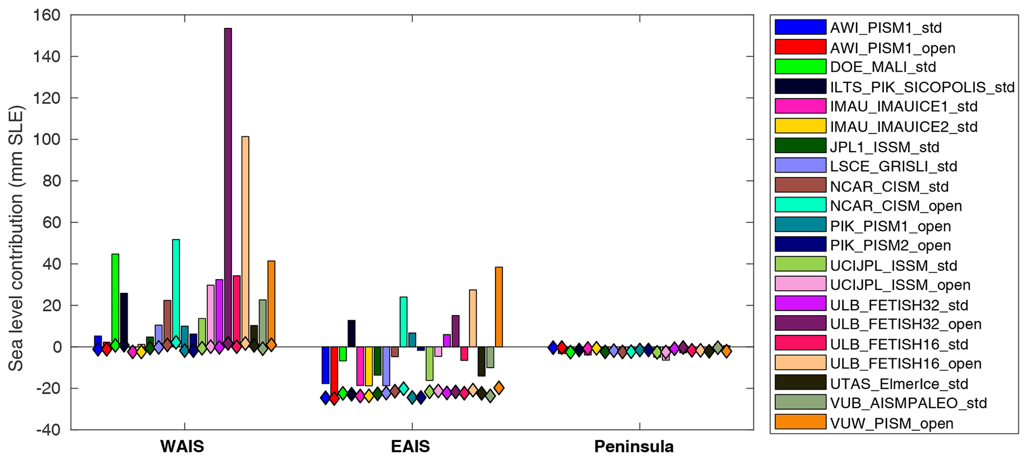
Figure 5 Regional change in volume above floatation (in mm SLE) and integrated SMB changes over the grounded ice (diamond shapes, in mm SLE) for the 2015–2100 period under medium RCP 8.5 forcing from NorESM1-M RCP 8.5 scenario (exp01 and exp05) relative to ctrl_proj.

Regions with the largest simulated changes can also be seen in Fig. 6, which shows the mean change in thickness and velocity between 2015 and 2100 for the 21 NorESM1-M simulations relative to ctrl_proj. Most Antarctic ice shelves thin by 20 m or more over the 86-year simulation, with the Ross ice shelf experiencing the largest thinning of about 75 m on average (Fig. 6a). This thinning does not propagate to the ice streams feeding the ice shelves, except for Thwaites Glacier in the Amundsen Sea sector and Totten Glacier in Wilkes Land. Many coastline regions, on the other hand, experience a small thickening, as is the case for the Antarctic Peninsula, Dronning Maud Land and Kemp Land, where the relative thickening is about 6 m next to the coast. Variations between the simulation are large and dominate the signal in many places (Fig. 6c). Changes in velocity (Fig. 6b) over ice shelves are more limited and not homogeneous, with acceleration close to the grounding line areas and slowdown close to the ice front, as observed for the Ross and Ronne-Filchner ice shelves. Some accelerations are observed on grounded parts of Thwaites, Pine Island and Totten glaciers as well. However, there is a large discrepancy in velocity changes among the simulations, and the standard deviation in velocity change is larger than the mean signal over most of the continent (Fig. 6d).

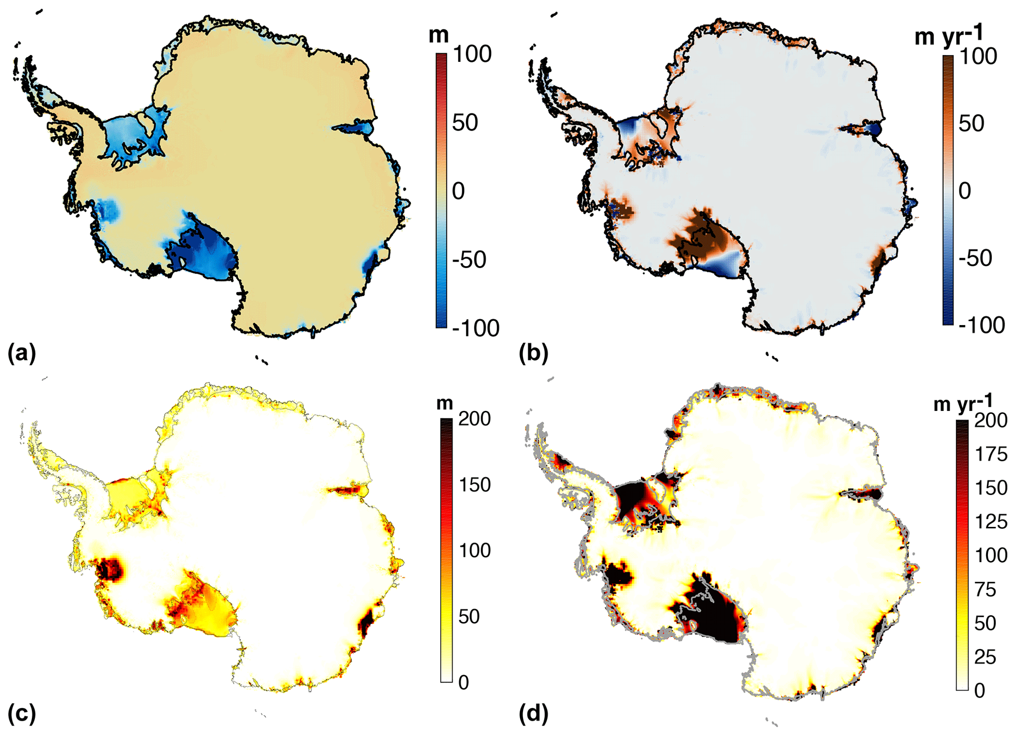
Figure 6 Mean (a and b) and standard deviation (c and d) of simulated thickness change (a and c, in m) and velocity change (b and d, in m yr⁻¹) between 2015 and 2100 under medium forcing from the NorESM1-M RCP 8.5 scenario (exp01 and exp05) relative to ctrl_proj.

4.4 Projections under RCP 8.5 scenario with various forcings

Outputs from six CMIP5 AOGCMs were used to perform RCP 8.5 experiments (see Table 1). Figure 7 shows the evolution of the simulated ice volume above floatation relative to ctrl_proj for all the individual RCP 8.5 simulations performed, as well as the mean values for each AOGCM. As seen above for NorESM1-M, changes are small for most simulations until 2050, after which differences between AOGCMs and ice flow simulations start to emerge. Runs with HadGEM2-ES lead to significant sea level rise, with a mean ice mass loss of 96 mm SLE (standard deviation: 72 mm SLE) for the 15 submissions of expA1 and expA5. Runs performed with CCSM4 show the largest ice mass gain, with a mean gain of 37 mm SLE (standard deviation: 34 mm SLE) for the 21 submissions of exp04 and exp08. Results for CSIRO-MK3 and IPSL-CM5A-MR are similar to CCSM4 at a continental scale but with slightly lower mass gain on average, while results from MIROC-ESM-CHEM simulate very little change, with a mean mass loss of 3 mm SLE.

Figure 7 Evolution of ice volume above floatation (in mm SLE) over the 2015–2100 period with medium forcing from the six CMIP5 models and RCP 8.5 scenario relative to ctrl_proj. Thin lines show results from individual ice sheet model simulations, and thick lines show mean values averaged for each CMIP5 model forcing. Bars on the right show the spread of results in ice flow models and mean values for the six CMIP5 forcings in 2100.

Figure 8 shows the regional differences in these contributions relative to ctrl_proj. Simulations suggest that WAIS will lose mass on average with four of the CMIP5 model forcings and gain mass with CSIRO-MK3 and IPSL-CM5A-MR. For the EAIS, results from five out of six CMIP5 model forcings lead to a mass gain on average, while HadGEM2-ES forcing causes a mass loss in the EAIS, with 23±26 mm SLE. Uncertainties are larger for WAIS than EAIS and larger for CMIP5 models that experience larger changes in ocean conditions. This is similar to what was observed in initMIP-Antarctica (Seroussi et al., 2019): in that study, changes in oceanic conditions (based on a forcing much simpler than is used in the current study) lead to a much larger spread in ice sheet evolution than changes in SMB. Changes in the Antarctic Peninsula lead to mass change between −6 and 6 mm SLE on average.

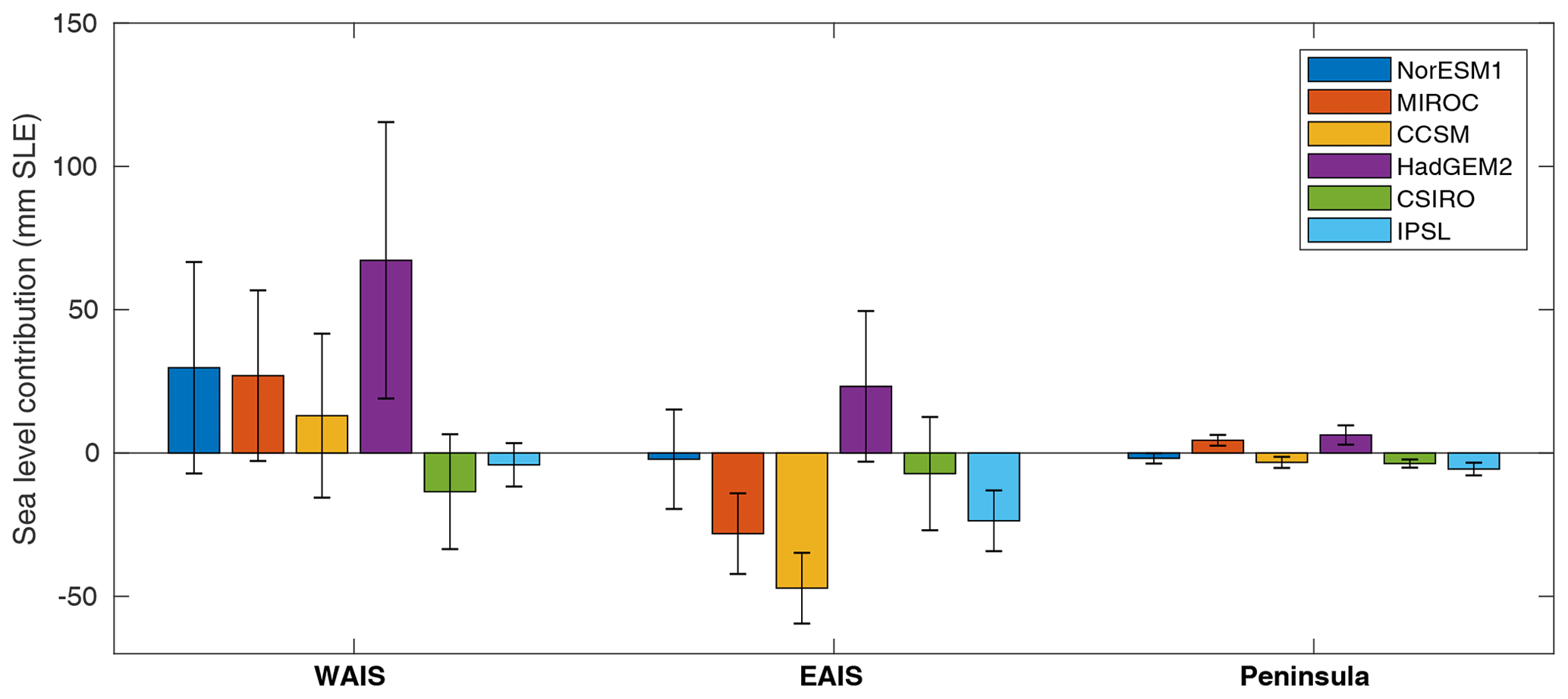
Figure 8 Regional change in volume above floatation (in mm SLE) for 2015–2100 from six CMIP5 model forcings under the RCP 8.5 scenario with median forcing, relative to ctrl_proj. Black lines show standard deviations.

4.5 Projections under RCP 8.5 and RCP 2.6 scenarios

Two CMIP5 models were chosen to run both RCP 8.5 and RCP 2.6 experiments: NorESM1-M and IPSL-CM5A-MR. Figure 9 shows the evolution of the Antarctic ice sheet under these two scenarios relative to ctrl_proj for both models. Only ice flow models that performed both RCP 8.5 and RCP 2.6 experiments were used to compare these scenarios, so two RCP 8.5 runs were not included, leading to the analysis of 20 NorESM1-M and 13 IPSL-CM5A-MR pairs of experiments.

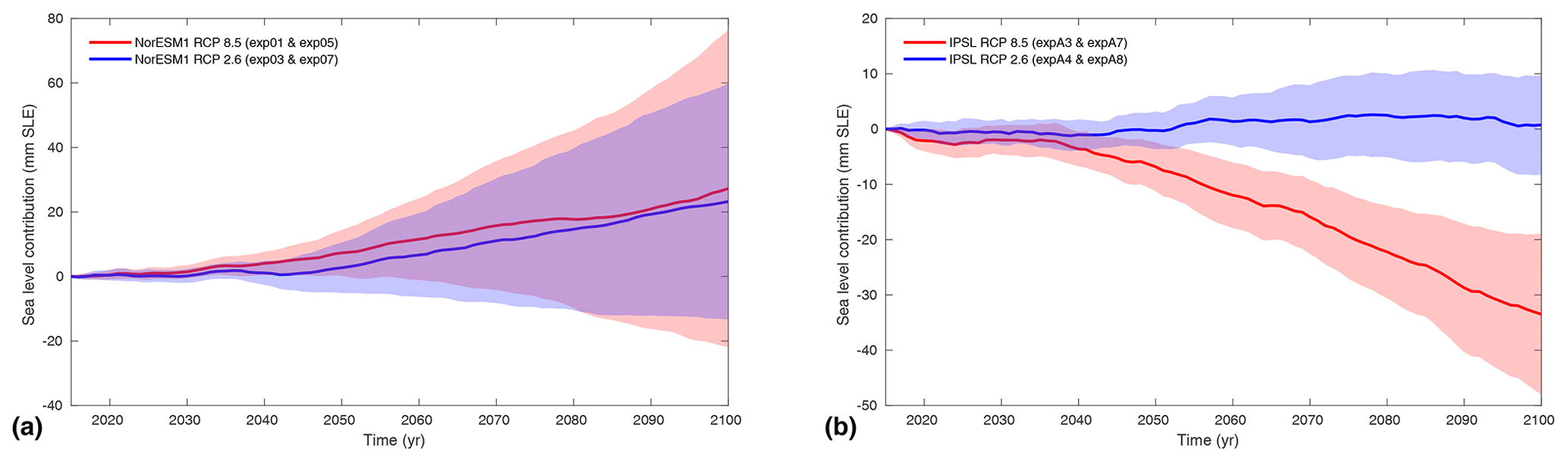
Figure 9 Impact of RCP scenario on projected evolution of ice volume above floatation for the NorESM1-M (a) and IPSL (b) models. Red and blue curves show mean evolution for RCP 8.5 and RCP 2.6, respectively, and the shaded background shows the standard deviation.

Results from NorESM show no significant change between the two scenarios in terms of simulated ice volume above floatation by 2100 (Fig. 9a). Both scenarios lead to a mean sea level contribution of about 25 mm SLE in 2100, with a higher standard deviation for the RCP 8.5 scenario (49 mm for RCP 8.5 and 37 mm for RCP 2.6). However, the overall similar behavior hides large regional differences revealed in Fig. 10a. The WAIS loses more mass while the EAIS gains more ice mass in RCP 8.5 compared to RCP 2.6. The additional SMB is greater for all regions under RCP 8.5 compared to RCP 2.6 (18 mm additional SLE in the EAIS and 2 mm additional SLE for the WAIS and Antarctic Peninsula) but is compensated for by a large dynamic response to ocean changes in both WAIS and EAIS.

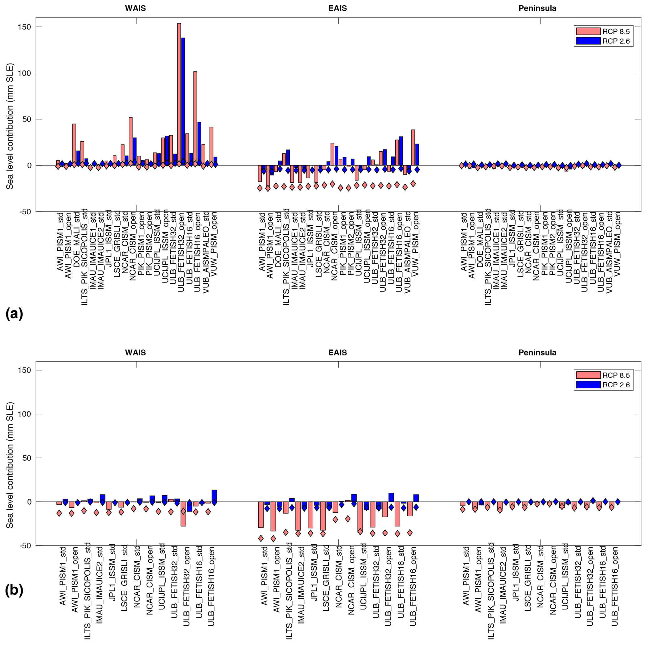
Figure 10 Regional change in volume above floatation (in mm SLE) and integrated SMB changes over the grounded ice (diamond shapes, in mm SLE) for 2015–2100 under the RCP 8.5 (red) and RCP 2.6 (blue) scenario forcings from NorESM1-M (a) and IPSL (b) relative to ctrl_proj from individual model simulations.

Simulations based on IPSL-CM5A-MR forcing, on the other hand, show significant differences in ice contribution to sea level at a continental scale. Ice contributes to $-\mathrm{33}\pm \mathrm{15}$ mm SLE for the RCP 8.5 scenario and 1±9 mm SLE for the RCP 2.6 scenario (Fig. 9). For RCP 2.6, the overall mass loss in the WAIS is compensated for by mass gain in the EAIS, leading to an overall ice mass that is nearly constant (Fig. 10). For RCP 8.5, there are large mass gains in all ice sheet regions as SMB increases significantly. Only a few simulations show mass loss of the WAIS relative to ctrl_proj. Similar to what is observed for NorESM1-M, the uncertainty is larger for RCP 8.5, as oceanic changes are more pronounced in this scenario.

Overall, these two CMIP5 models respond very differently to increased carbon concentrations, which is reflected in the differences in ice sheet evolution.

4.6 Impact of ice shelf basal melt parameterization

All of the RCP 8.5 experiments were simulated with the open (exp01-04) and standard (exp05-08) melt frameworks (Table 1). The standard framework allows us to assess the uncertainty associated with ice flow models when the processes controlling ice–ocean interactions are fixed. The open framework, in contrast, allows for additional uncertainties due to the physics of ice–ocean interactions that remain a subject of active research (Asay-Davis et al., 2017; Favier et al., 2019). We now investigate the effects of these different approaches on simulation results.

Figure 11 shows the cumulative ocean-induced basal melt and the change in ice volume above floatation between 2015 and 2100 and relative to ctrl_proj for the six RCP 8.5 experiments and for the 8 and 14 submissions using the open and standard melt frameworks, respectively. The basal melt applied in the standard framework is higher than the basal melt resulting from the open framework for about half of the experiments and Antarctic regions and lower for the other half. However, despite the similar melt rates applied, the sea level contribution relative to ctrl_proj is higher (either more mass loss or less mass gain) in the open framework than in the standard framework in the WAIS and EAIS, except for IPSL in the WAIS. Numbers are small and similar in the Antarctic Peninsula. The mean additional sea level contribution (either more mass loss or less mass gain) simulated in the open framework is 25 mm SLE for WAIS and 20 mm for EAIS. The standard deviation of both basal melt and sea level contribution is larger in the open melt framework (see Fig. 11), which is expected given the additional flexibility in the melt parameterization and the wide range of melt parameterizations used in the open framework (see Table 3).

Figure 11 Regional change in integrated basal melt (a, in Gt) and volume above floatation (b, in mm SLE) for 2015–2100 under medium forcing from the six CMIP5 AOGCMs using RCP 8.5 forcing, relative to ctrl_proj for the open (solid patterns) and standard basal melt (dashed patterns) frameworks. Black lines show the standard deviations.

4.7 Impact of ice shelf melt uncertainties

The effect of uncertainties in the melt rate parameterization is assessed exclusively for the standard melt parameterization framework, for which different choices of parameters can be used in a similar way by all models (exp05, exp09, exp10 and exp13 in Table 1). Here we assess the effect of two sources of uncertainty that affect the choice of γ₀ and the regional δ_T values. The melt parameterization provides a distribution of γ₀, and the median value is used for most experiments (see Table 1). Two experiments (exp09 and exp10) use the 5th and 95th percentile values of the distribution to estimate the effect of parameter uncertainty on basal melt and ice mass loss. A third experiment investigates the effect of the dataset used to calibrate the melt parameterization (exp13): instead of using all the melt rates and ocean conditions around Antarctica, it uses only the high melt values near the Pine Island ice shelf grounding line (“PIGL” coefficient; see Sect. 2.3), which results in γ₀ that is an order of magnitude higher (Jourdain et al., 2020). All of these experiments are based on NorESM1-M and RCP 8.5, so the applied SMB is similar in all experiments (only the basal melt differs). The initial basal melt is calibrated to be equal to observed values (Rignot et al., 2013; Depoorter et al., 2013) in each case and for each Antarctic basin, so only the initial distribution of melt and its evolution in time vary while its total initial magnitude is similar.

Figure 12a shows the effect of using the 5th, 50th and 95th percentile values of the γ₀ distribution for models that performed these three experiments. The total melt starts from similar values but diverges quickly as ocean conditions change. By 2100, the additional mean total melt applied relative to the control experiment is 3030 Gt yr⁻¹ for the median value, while it is 2540 and 3460 Gt yr⁻¹, respectively, for the 5th and 95th percentile values of the γ₀ distribution. While these differences represent about 15 % of the additional melt applied, they fall largely within the spread of basal melt values applied for the median γ₀ for the different simulations (caused by the different model geometries) and are smaller than interannual variations. Impacts of these changes on ice dynamics are shown in Fig. 12c. The mean sea level contribution with the median γ₀ is 6.9 mm SLE, while it is −0.7 and 12.0 mm SLE in 2100 for the 5th and 95th percentile compared to the ctrl_proj experiment. The overall evolution of Antarctica remains similar only for a couple of decades, at which point the three experiments start to diverge.

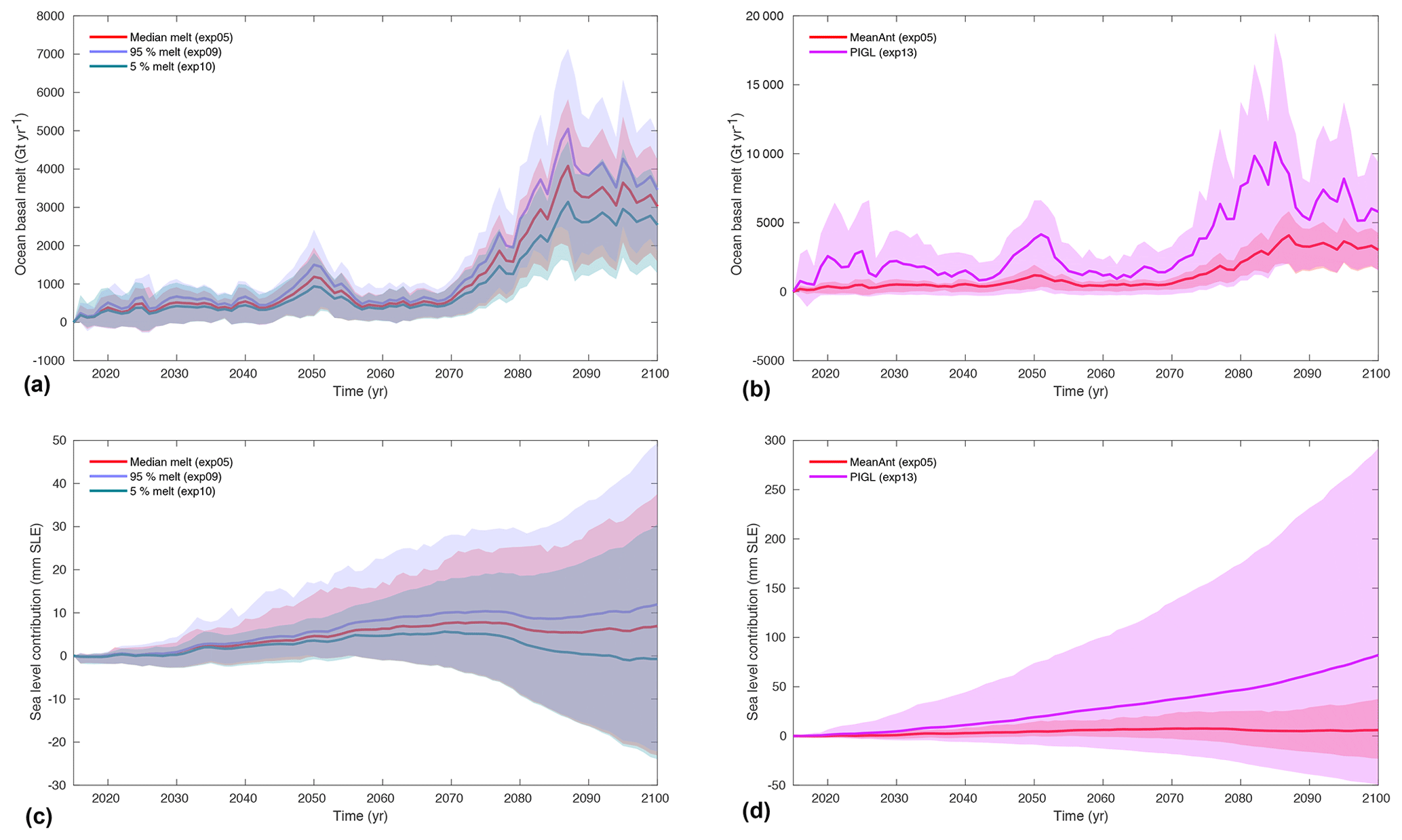
Figure 12 Impact of basal melt parameterization (a and c; 5th, 50th and 95th percentile values of γ₀ distribution) and calibration (b and d; “MeanAnt” and “PIGL” calibrations) on basal melt evolution (a and b, in Gt yr⁻¹) and ice volume above floatation (c and d, in mm SLE) relative to ctrl_proj over 2015–2100. Lines show the mean values, and the shaded background shows the simulation spreads. Note that the y axes differ in all plots.

Figure 12 also highlights the role of the calibration method. The “MeanAnt” and “PIGL” experiments (exp05 and exp13) start with similar total melt values and are both calibrated to be in agreement with current observations of melt (because models have initial geometries that differ from observations, they can have some differences in the amount of total initial melt). The total melt diverges between the two experiments after just a few years, and continues to diverge during the 21st century as ocean conditions and ice shelf configurations change, reaching 3030 and 5790 Gt yr⁻¹ on average in 2100 for the “MeanAnt” and “PIGL” experiments relative to the ctrl_proj experiment (Fig. 12b), respectively. The effect on ice dynamics and sea level is large, with a 12 times larger mean contribution to sea level by 2100 relative to ctrl_proj for the “PIGL” experiment, reaching a mean SLE contribution of 30 mm; see Fig. 12d. This is the simulation with the greatest amounts of ice loss, with models predicting mass loss of up to 30 cm SLE by 2100 compared to the ctrl_proj experiment. This melt parameterization causes larger melt rates close to grounding lines and higher sensitivity to ocean warming, as γ₀ is an order of magnitude larger for the “PIGL” parameterization than for the “MeanAnt” parameterization. Thus, this run represents an upper end to plausible values for sub-shelf melting, yet it is calibrated to simulate initial basal melting in agreement with present-day observations. It also highlights the nonlinear ice sheet response to submarine melt forcing: the doubling of basal melt relative to the ctrl_proj experiment leads to a 10 times greater ice mass loss relative to the ctrl_proj results.

4.8 Impact of ice shelf collapse

The effect of ice shelf collapse is tested with exp11 and exp12 for the open and standard frameworks, respectively (Table 1). These experiments are based on outputs from CCSM4 and are similar to exp04 and exp08: the SMB and ocean thermal forcing are similar, so the two sets of experiments only differ by the inclusion of ice shelf collapse. As mentioned in Sect. 2.4, the processes included in the response of the tributary ice streams feeding into these ice shelves is left to the judgment of modeling groups. However, no group included the marine ice cliff instability (Pollard et al., 2015) following ice shelf collapse. Only the 14 simulations (including 4 open and 10 standard melt parameterizations) that performed the ice shelf collapse experiments are included in the analysis of ice shelf collapse. Results from 7 simulations of exp04 and exp08 were therefore excluded from the ensemble with no ice shelf collapse.

As shown in Nowicki et al. (2020), the presence of significant liquid water on the surface of ice shelves is limited to less than 60 000 km² until 2040, so ice shelf collapse is marginal. Starting in 2040, it rapidly increases, reaching 460 000 km² by 2100. The evolution of ice shelf extent in the ice sheet simulations reflects this evolution: Fig. 13a shows the evolution of ice shelf extent for the CCSM4 simulations with and without ice shelf collapse. As the external forcings are similar in both runs, the difference comes from the ice shelf collapse and the response to this collapse. In the simulations without collapse, ice shelf extent remains relatively constant, with 11 000 km² change on average compared to ctrl_proj on average. When ice shelf collapse is included, ice shelf extent is reduced by 66 000 km² between 2015 and 2100 compared to the ctrl_proj runs on average for the 14 ice sheet simulations.

While ice shelf collapse does not directly contribute to sea level rise, the dynamic response of the ice streams to the collapse leads to an average of 28 mm SLE difference between the two scenarios relative to the ctrl_proj experiment (Fig. 13a). These changes occur largely over the Antarctic Peninsula, next to George VI ice shelf, but also on Totten Glacier (see Fig. 14a). Including ice shelf collapse leads to a concurrent acceleration of up to 100 m yr⁻¹ in these same regions (see Fig. 14b). However, large uncertainties dominate these model responses.

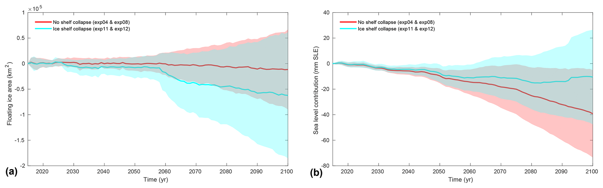
Figure 13 Evolution of basal melt (a, in Gt yr⁻¹) and ice volume above floatation relative to ctrl_proj (b, in mm SLE) without (red) and with (cyan) ice shelf collapse over the 2015–2100 period under the CCSM4 RCP 8.5 forcing. Lines show the mean values, and the shaded background shows the standard deviations. Note the negative values of sea level contribution and therefore mass gain in panel (b).

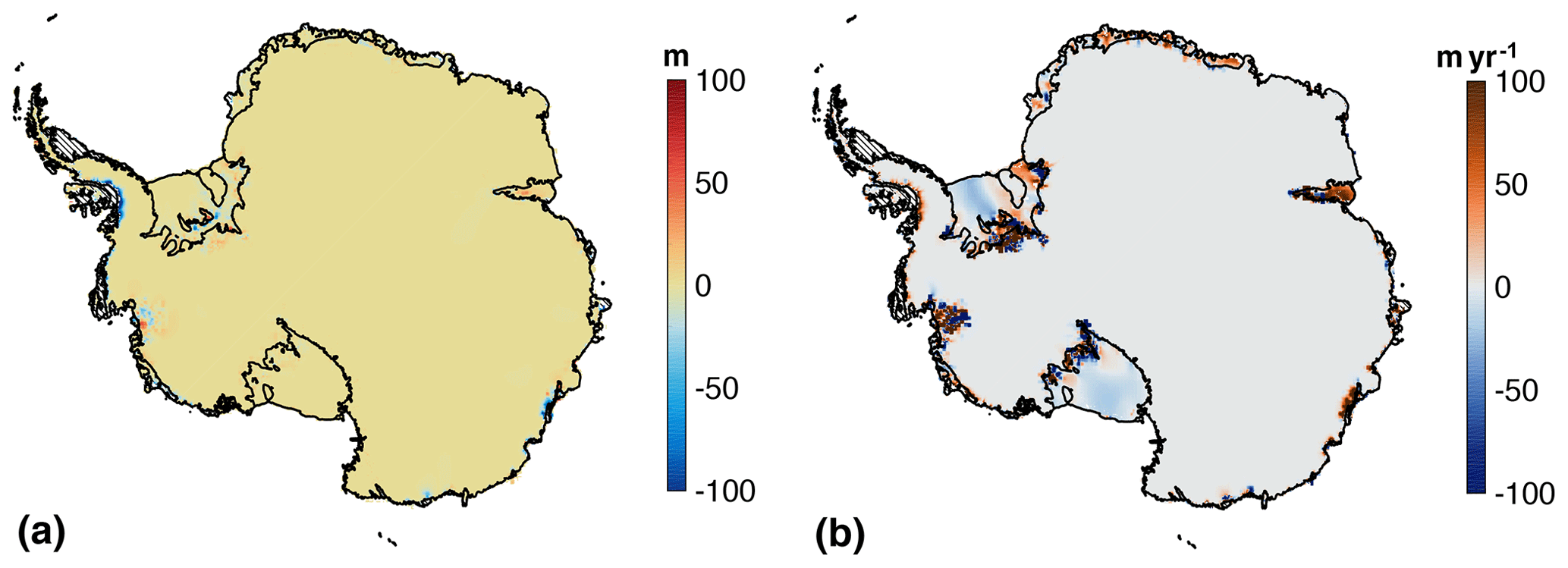
Figure 14 Mean simulated thickness change (a, in m) and velocity change (b, in m yr⁻¹) between 2015 and 2100 with ice shelf collapse under CCSM4 RCP 8.5 scenario (exp11 and exp12) relative to similar experiments without ice shelf collapse (exp04 and exp08). Hatched areas show areas experiencing ice shelf collapse by 2100.

The ice shelf collapse experiments are based on CCSM4, as this model shows the largest potential for ice shelf collapse out of the six AOGCMs selected (Nowicki et al., 2020). Similar experiments performed with other AOGCMs are therefore expected to show a lower response to ice shelf collapse.

5 Discussion

ISMIP6-Antarctica projections under the RCP 8.5 scenario show a large spread of Antarctic ice sheet evolution over 2015–2100, depending on the ice flow model adopted, the CMIP5 forcings applied, the ice sheet model processes included, and the form and calibration of the basal melt parametrization. The results presented here suggest the contribution to sea level with the “MeanAnt” calibration in response to this scenario varies between a sea level drop of 7.6 cm and a sea level increase of over 27 cm, compared to a constant climate similar to that of the past few decades. Contributions up to 30 cm are also simulated when the melt parameterization is calibrated to produce high melt rates near Pine Island's grounding line (see Sect. 4.7). The latter parameterization is calibrated with the same present-day observations but has a much stronger sensitivity to ocean forcing (Jourdain et al., 2020), leading to more rapid increases in basal melting as ocean waters in ice shelf cavities warm. As observations of ocean conditions within ice shelf cavities and resulting ice shelf melt rates remain limited, these numbers cannot be excluded from consideration.

All the simulations results reported here describe Antarctic mass loss relative to that from a constant climate, so the mass loss trend over the past few decades needs to be added to obtain a total Antarctic contribution to sea level through 2100. The recent IMBIE assessment estimated the Antarctic mass loss to be between 38 and 219 Gt yr⁻¹, depending on the time period considered (Shepherd et al., 2018), which corresponds to a cumulative mass loss of 9 and 52 mm over 2015–2100. Adding this to the range of Antarctic mass loss simulated as part of ISMIP6 gives a range of between −6.7 and 35 cm SLE. These numbers cover the wide range of results previously published (e.g., Edwards et al., 2019; DeConto and Pollard, 2016; Schlegel et al., 2018; Golledge et al., 2019) but do not reproduce the highest contributions up to 1 m previously reported. These numbers show less spread than the simulations performed under the SeaRISE experiments, mostly due to the lower basal melt anomalies applied under ice shelves (Bindschadler et al., 2013; Nowicki et al., 2013a). They are also similar to numbers presented by Pachauri et al. (2014), where the likely range (5 %–95 % of model range) of Antarctic contribution to global mean sea level rise between the 1986–2005 period and 2100 under the RPC 8.5 scenario was between −8 and 14 cm.

The simulated response of the ice sheet to changes in ocean forcings has significant spatial variation, suggesting that some sectors of the ice sheet are significantly more vulnerable to changes in ocean circulation than others. Figure 15 shows the sensitivity of the 18 Antarctic basins (Rignot et al., 2019) to changes in oceanic conditions using all the RCP 8.5 experiments performed by all the ice sheet models based on medium ocean conditions. The dynamic mass loss (total ice above floatation mass loss minus SMB change) between 2015 and 2100 is represented as a function of the cumulative ocean-induced melt over the same period, both relative to ctrl_proj. The Amundsen Sea sector and Wilkes Land show the largest dynamic response and therefore sensitivity to increase in ocean-induced basal melting. Glaciers feeding the west side of the Ross ice shelf show very small response despite relatively large increased basal melt, as only very narrow glaciers protected by wide stabilizing ridges cross the Transantarctic Mountains to enter this area (Morlighem et al., 2020). The Ross ice streams and glaciers feeding the Ronne ice shelf also experience limited dynamic response to increased basal melt. For the other regions, none of the CMIP5 forcing used predicted a large increase in ocean-induced melt by 2100, so we cannot conclude on the sensitivity of these sectors to oceanic forcings.

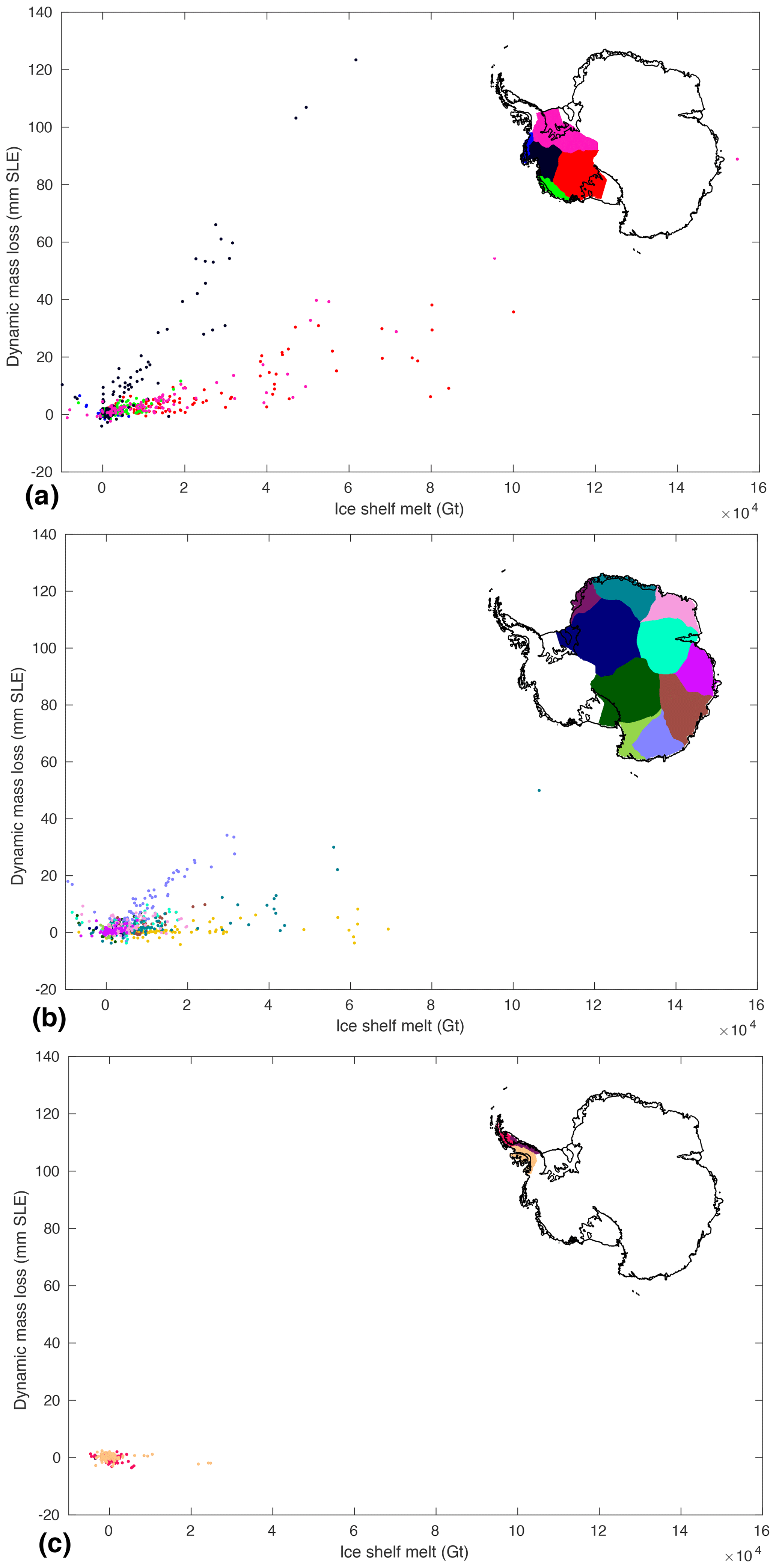
Figure 15 Sensitivity of individual basins to increased ocean basal melt over the 2015–2100 period: (a) the Antarctic Peninsula, (b) WAIS and (c) EAIS. The dynamic mass loss is approximated as to the total mass loss minus the cumulative anomaly in surface mass balance. It is shown as a function of cumulative ocean-induced basal melt anomaly over the same period for each of the 18 main Antarctic basins (Rignot et al., 2019) and for all RCP 8.5 experiments with medium ocean forcing. Dynamic change and basal melt are both relative to ctrl_proj experiment. Antarctic maps show the location of the 18 Antarctic basins.

The large spread in Antarctic ice sheet projections reported here contrasts with the relatively narrow range of projections reported as part of ISMIP6 in Goelzer et al. (2020) for the Greenland ice sheet. We attribute this difference to the dominant role of SMB in driving future evolution of Greenland and the more constrained forcing applied for ice front retreat in Greenland, in which most models used a prescribed a retreat rate.

For Antarctica, we find that uncertainties in the sea level estimates come from the spread in AOGCM forcing (see Sect. 4.4), the melt parameterization adopted and its calibration (see Sects. 4.6 and 4.7), and the spread caused by the choices made by the ice flow models for their initialization and the physical processes included (see Sect. 4.3 and Seroussi et al., 2019). All of these sources of uncertainty affect the results, and uncertainties in ocean conditions and their conversion into basal melt rates through parameterization lead to the largest spread of results, especially when different datasets are used for parameter calibration. Additional Antarctic mass losses of more than 20 cm SLR by 2100 under RCP 8.5 compared to constant climate conditions are reached only for the simulations based on the PIGL calibration (Fig. 12) or as part of the open melt framework. Furthermore, not only does the magnitude of basal melt influence Antarctic dynamics, but the spatial distribution of melt rates has a strong effect on the results, as observed when comparing the open and standard experiments (Sect. 4.6). These findings are similar to those described by Gagliardini et al. (2010) based on idealized model configurations and highlight the need to acquire more observations and to use coupled ice–ocean models to better understand ice–ocean interactions and represent them in ice flow models (Seroussi et al., 2017; Favier et al., 2019).

The results presented here do not include any weighting of the ice flow models based on their agreements with observations or the number of simulations submitted. As explained in previous studies (Goelzer et al., 2017, 2018; Seroussi et al., 2019), the range of initialization techniques adopted by models leads to various biases. Some models are initialized with a long paleoclimate spin-up, giving limited spurious trends but an initial configuration further from the observed state, whereas other models initialized with data assimilation of present-day observations can capture these conditions accurately but often have nonphysical trend in their evolution. Assigning weights to different models is therefore a complicated question that is not addressed in the present study. This choice might lead to an overrepresentation of the models that submitted several contributions but is similar to that adopted within the larger CMIP framework.

The simulations performed as part of ISMIP6-Antarctica projections represent a significant improvement compared to previous intercomparisons of Antarctic evolution, especially in terms of the treatment of ice shelves, grounding line evolution, and ocean-induced basal melt that were not always included in previous continental Antarctic models (Bindschadler et al., 2013; Nowicki et al., 2013a). This progress is representative of improvements made to ice flow models over the past decade (Pattyn et al., 2018). Ice shelf melt parameterizations have been improved to reproduce the main features of basal melt simulated in ocean models and captured in observations. They are based on simulated ocean conditions extrapolated in ice shelf cavities, while uniform prescribed values were used in previous efforts (Nowicki et al., 2013a). Grounding line migration and model resolution have been significantly improved (see Table 3) and an increasing number of models are simulating ice front migrations. However, several limitations remain, regarding both external forcings (Nowicki and Seroussi, 2018) and ice flow models (Pattyn et al., 2018). SMB forcing from AOGCMs generally has a coarse resolution, and no regional model was used to downscale the forcing, unlike what was done for Greenland (Nowicki et al., 2020; Goelzer et al., 2020), so SMB might not be well captured in regions with steep surface slopes. The inclusion of surface elevation feedbacks (Helsen et al., 2012) was left to the discretion of ice modeling groups, and no model included one, so this positive feedback was neglected in the present simulations. Because CMIP5 AOGCMs do not include ocean circulation under ice shelves, several simplifying assumptions must be made to estimate ocean conditions in ice shelf cavities (Jourdain et al., 2020). Ice–ocean interactions in ice shelf cavities are poorly observed and constrained (Dutrieux et al., 2014; Jenkins et al., 2018; Holland et al., 2019), leading to additional limitations on the representation of ocean-induced sub-shelf melt. While pan-Antarctic estimates of basal melt have been produced (Depoorter et al., 2013; Rignot et al., 2013), we are missing time series of basal melt at that scale and coinciding observations of oceanic conditions. Despite the progress in ice sheet numerical modeling over the last decade (Pattyn et al., 2018; Goelzer et al., 2017), significant limitations remain in our understanding of basal sliding (Brondex et al., 2019), basal hydrology (De Fleurian et al., 2018), calving (Benn et al., 2017) and interaction with solid Earth (Gomez et al., 2015; Larour et al., 2019). Finally, there was no incentive for models to represent the changes recently observed in Antarctica. However, as a variety of remote sensing observations are starting to provide time series of ice sheet changes over the recent past, it is becoming increasingly important to assess the ability of models to reproduce such observations in order to gain confidence in the projections.

The analysis of the simulations conducted as part of ISMIP6-Antarctic are projections that are presented here as relative to the ctrl_proj control experiments and therefore represent estimates of mass loss caused by variations in climate compared to a scenario with a constant climate. It was decided that using results of ice flow simulations directly, without subtracting the trend from a control run, is not yet appropriate given the large trend in the historical simulations and control experiments (Fig. 1). Such a trend does not represent recent physical changes but rather limitations in observations (Seroussi et al., 2011), external forcings (Nowicki and Seroussi, 2018), ice flow models (Pattyn et al., 2018), and procedures used to initialize ice flow models (Seroussi et al., 2019; Nowicki and Seroussi, 2018; Goldberg et al., 2015). As ice sheets respond nonlinearly to changes, such an approach introduces a bias in the ice response, but this approach was deemed to be the most appropriate approach given current limitations. This same approach has been adopted in other recent ice flow modeling studies (e.g., Nowicki et al., 2013a, b; Schlegel et al., 2018; Goelzer et al., 2020). The choice of AOGCMs was made to cover a large range of responses to RCP scenarios but is not representative of the mean changes exhibited by CMIP5 AOGCMs (Barthel et al., 2020). As a result, we expect that the spread of model response represented here covers the diversity of AOGCM outputs. However, computing mean values using different AOGCMs should be avoided, as only a few AOGCMs were sampled. Finally, all the results presented here are based on CMIP5 AOGCMs. Additional results based on CMIP6 AOGCMs will be presented in following publications.

6 Conclusions

Here we present simulations of the Antarctic ice sheet evolution between 2015 and 2100 from a multi-model ensemble, as part of the ISMIP6 framework. Ice sheet models from 13 international ice sheet modeling groups are forced with outputs from AOGCMs chosen to represent a large spread of possible evolution of oceanic and atmospheric conditions around Antarctica over the 21st century. Simulation results suggest that the Antarctic ice sheet could contribute between −7.6 and 30.0 cm of SLE under the RCP 8.5 scenario compared to a scenario of constant conditions representative of the past decade. Climate models suggest significant increases in surface mass balance that are partially balanced by dynamic changes in response to ocean warming. Simulations suggest strong regional differences: WAIS loses mass under most scenarios and for all ice sheet models, as the increase in surface mass balance remains limited but the increase in ice discharge are large. EAIS, on the other hand, gains mass in many simulations, as dynamic mass loss is too limited to compensate for the large increase in surface mass balance. The regions most vulnerable to changes in the simulations are the Amundsen Sea sector in West Antarctica and Wilkes Land in East Antarctica. Simulations of the Antarctic ice sheet evolution under the RCP 2.6 scenario contribute less to sea level rise and have a smaller spread in SLE contribution between −1.4 and 15.5 cm relative to a constant forcing, with less surface mass balance increase and a smaller dynamic response. The main sources of uncertainties highlighted in this study are the physics of ice flow models, the climate conditions used to force the ice sheet and the representation of ocean-induced melt at the base of ice shelves.

Appendix A: Requested outputs

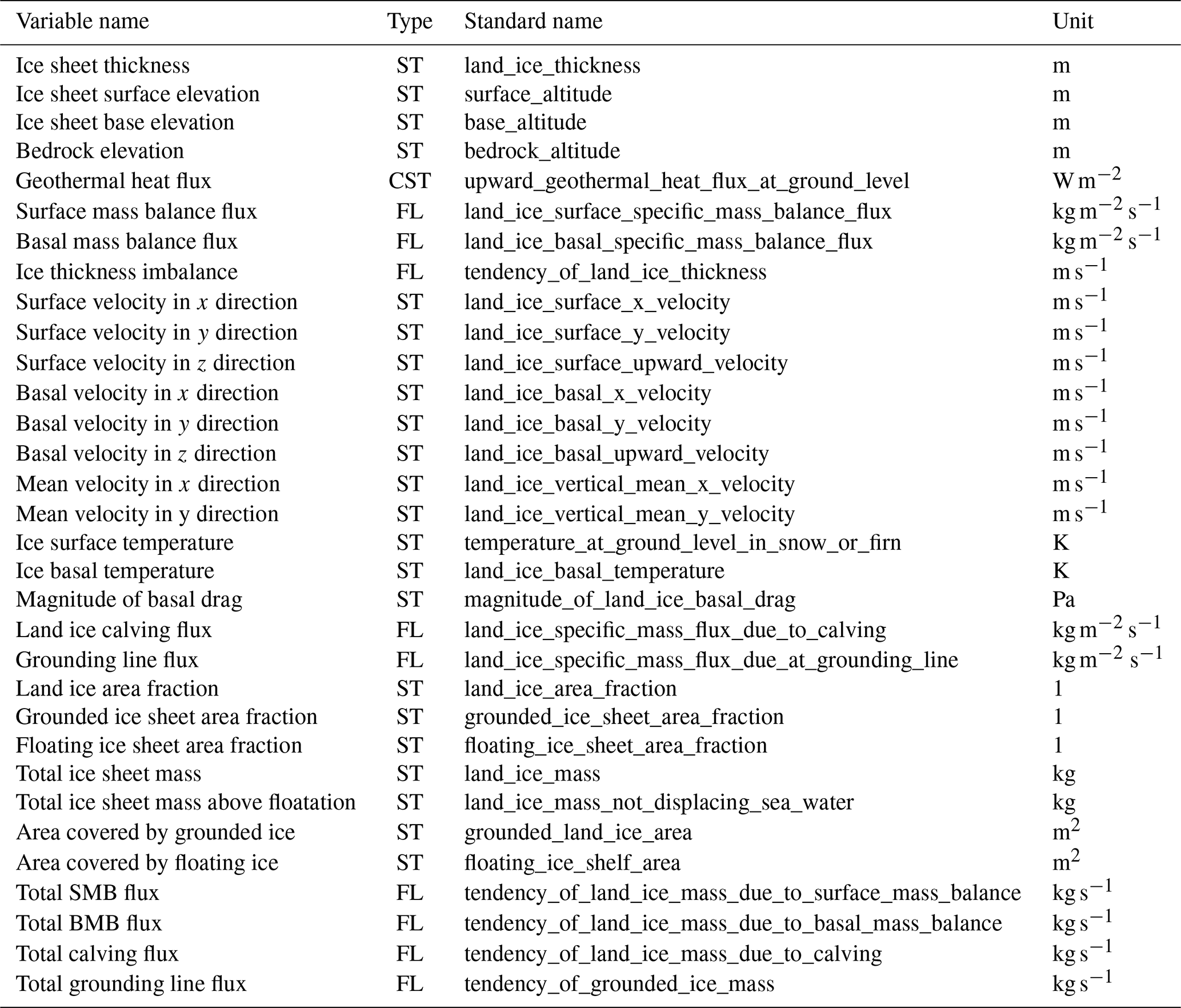
The model outputs requested as part of ISMIP6 are listed in Table A1. Annual values were submitted for both scalar and two-dimensional variables. Flux variables reported are averaged over calendar years, while state variables are reported at the end of calendar years.

Table A1 Data requests for Antarctica projections. ST stands for state variable, FL stands for flux variable and CST stands for constant.

Appendix B: Summary of initial state and control run evolution

We report here the scalar values of simulated Antarctic ice mass, ice mass above floatation, ice extent, and ice shelf extent in Tables B1 and B2. Values are reported at the beginning of January 2015, when the experiments start in Table B1. We also report the evolution of ice mass, ice mass above floatation, ice extent and ice shelf extent during the ctrl_proj simulation (between 2015 and 2100) in Table B2.

Table B1 Simulated Antarctic ice mass, ice mass above floatation, total ice extent and floating ice extent at the beginning of the experiments (January 2015).

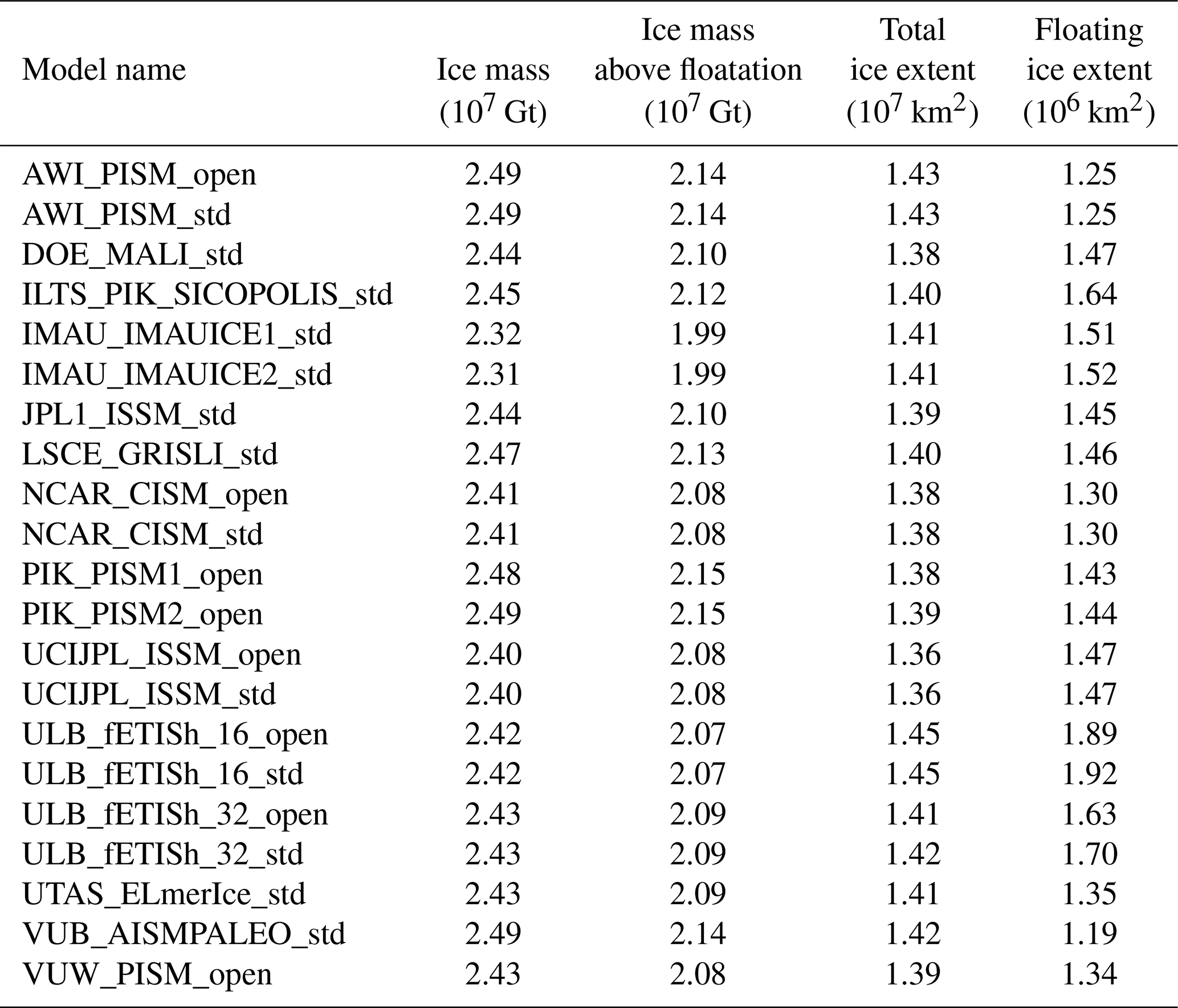
Table B2 Simulated Antarctic ice mass, ice mass above floatation, total ice extent and floating ice extent change during the ctrl_proj experiment (between 2015 and 2100).

Appendix C: Ice flow model initialization and characteristics

The descriptions below summarize the initialization procedure and main characteristics of the different ice flow modeling groups.

C1 AWI_PISM

The AWI_PISM ice sheet model is based on the Parallel Ice Sheet Model (PISM, Bueler and Brown, 2009; Winkelmann et al., 2011; Aschwanden et al., 2012) version 1.1.4 with modifications for ISMIP6. PISM solves a hybrid combination of the non-sliding shallow ice approximation (SIA) and the shallow shelf approximation (SSA) for grounded ice, where the SSA solution acts as a sliding law, and only the SSA for floating ice. PISM also solves for enthalpy to account for the temperature and water content of the ice in the rheology. The model uses a structured rectangular grid with a uniform horizontal resolution of 8 km (16 km early in the spin-up) and 81 vertical z-coordinate levels that are refined towards the base. The total ice domain height is 6000 m with an additional heat conducting bedrock layer of 2000 m thickness (21 equal levels). The calving front can evolve freely on a sub-grid scale (Albrecht et al., 2011). In addition to calving below a certain thickness threshold (here 150 m), a kinematic first-order calving law, called eigen-calving (Levermann et al., 2012), is utilized with the calving parameter K=10¹⁷ m s. Floating ice that extends far into the open ocean (seafloor elevation reaches 2000 m below sea level) is also calved off. The grounding line position is determined using hydrostatic equilibrium. Basal friction in partially grounded cells is weighted according to the grounded area fraction (Feldmann et al., 2014). The nonlocal quadratic melt scheme and the related datasets provided by ISMIP6 are used to compute the ice shelf basal melt in the spin-up and all “standard” experiments. For the “open” experiments, the local quadratic melt scheme is used. Ice shelf basal melt is applied on a sub-grid scale.

To initialize the model, an equilibrium-type spin-up based on steady present-day climate has been performed. Atmospheric forcing (2 m air temperature and precipitation) is the multi-annual mean 1995–2014 (ISMIP6 reference period) from RACMO2.3p2 (van Wessem et al., 2018). For the surface mass balance, a positive degree-day scheme (Huybrechts and de Wolde, 1999; Martin et al., 2011) is used. Geothermal heat flux is from (Shapiro and Ritzwoller, 2004) and the bedrock elevation is fixed in time. The ocean is forced with the present-day ocean forcing field provided by ISMIP6. The spin-up consists of an initialization with idealized temperature–depth profiles, a 100-year geometry relaxation run and a 200 kyr thermo-mechanically coupled run with fixed geometry for thermal equilibration. For those stages, the non-sliding SIA is used on a 16 km horizontal grid. After re-gridding the output (except the geometry) onto the final 8 km grid, the model runs for 30 kyr using full model physics and a freely evolving geometry. The initial ice sheet geometry for the spin-up is based on Bedmap2 (Fretwell et al., 2013) and is refined in the Recovery Glacier area with additional ice thickness datasets (Humbert et al., 2018; Forsberg et al., 2018). The historical simulation from January 2005 until the end of December 2014 employs the NorESM1-M-RCP8.5 atmospheric and oceanic forcing.

C2 DOE_MALI

MPAS-Albany Land Ice (MALI) (Hoffman et al., 2018) uses a three-dimensional, first-order “Blatter–Pattyn” momentum balance solver solved using finite-element methods (Tezaur et al., 2015). Ice velocity is solved on a two-dimensional map plane triangulation extruded vertically to form tetrahedra. Mass and tracer transport occur on the Voronoi dual mesh using a mass-conserving finite volume first-order upwinding scheme. Mesh resolution is 2 km along grounding lines, in all marine regions of West Antarctica and in marine regions of East Antarctica where present-day ice thickness is less than 2500 m to ensure that the grounding line remains in the fine-resolution region even under full retreat of West Antarctica and large parts of East Antarctica. Mesh resolution coarsens to 20 km in the ice sheet interior and no greater than 6 km in the large ice shelves. The horizontal mesh has 1.6 million cells. The mesh uses 10 vertical layers that are finest near the bed (4 % of total thickness in deepest layer) and coarsen towards the surface (23 % of total thickness in shallowest layer). Ice temperature is based on results from Van Liefferinge and Pattyn (2013) and held fixed in time. The model uses a linear basal friction law with spatially varying basal friction coefficient. The basal friction of grounded ice and the viscosity of floating ice are inferred to best match observed surface velocity (Rignot et al., 2011) using an adjoint-based optimization method (Perego et al., 2014) and then kept constant in time. The grounding line position is determined using hydrostatic equilibrium, with sub-element parameterization of the friction. Sub-ice-shelf melt rates come from Rignot et al. (2013) and are extrapolated across the entire model domain to provide nonzero ice shelf melt rates after grounding line retreat. The surface mass balance is from the RACMO2.1 1979–2010 mean (Lenaerts et al., 2012). Maps of surface and basal mass balance forcing are kept constant with time in the ctrl_proj experiment. Time-varying anomalies of surface and basal mass balance relative to the original fields are applied in all other experiments. The ice front position is fixed at the extent of the present-day ice sheet. After initialization, the model is relaxed for 99 years so that the geometry and grounding lines can adjust.

C3 ILTS_PIK_SICOPOLIS

The model SICOPOLIS version 5.1 (Greve and SICOPOLIS Developer Team, 2019; http://www.sicopolis.net/, last access: 6 July 2020) is applied to the Antarctic ice sheet with hybrid shallow-ice–shelfy-stream dynamics for grounded ice (Bernales et al., 2017) and shallow-shelf dynamics for floating ice. Ice thermodynamics is treated with the melting-CTS (cold-temperate transition surface) enthalpy method (ENTM) by Greve and Blatter (2016). The ice surface is assumed to be traction-free. Basal sliding under grounded ice is described by a Weertman–Budd-type sliding law with sub-melt sliding (Sato and Greve, 2012) and subglacial hydrology (Kleiner and Humbert, 2014; Calov et al., 2018). The model is initialized by a paleoclimatic spin-up over 140 000 years until 1990, forced by Vostok δD converted to ΔT (Petit et al., 1999), in which the topography is nudged towards the present-day topography to enforce a good agreement (Rückamp et al., 2019). The basal sliding coefficient is determined individually for the 18 IMBIE-2016 basins (Rignot and Mouginot, 2016) by minimizing the RMSD between simulated and observed logarithmic surface velocities. The historical run from 1990 until 2015 employs the NorESM1-M-RCP8.5 atmospheric and oceanic forcing. For the last 2000 years of the spin-up, the historical run and the future climate simulations, a regular (structured) grid with 8 km resolution is used. In the vertical, we use terrain-following coordinates with 81 layers in the ice domain and 41 layers in the thermal lithosphere layer below. The present-day surface temperature is parameterized (Fortuin and Oerlemans, 1990), the present-day precipitation is by Arthern et al. (2006) and Le Brocq et al. (2010), and runoff is modeled by the positive-degree-day method with the parameters by Sato and Greve (2012). The 1960–1989 average SMB correction that results diagnostically from the nudging technique is used as a prescribed SMB correction for the future climate simulations. The bed topography is Bedmap2 (Fretwell et al., 2013), the geothermal heat flux is by Martos et al. (2017), and isostatic adjustment is included using an elastic-lithosphere–relaxing-asthenosphere (ELRA) model (parameters by Sato and Greve, 2012). Present-day ice-shelf basal melting is parameterized by the ISMIP6 standard approach (Eq. 1). A more detailed description of the setup, which is consistent with the one used for the LARMIP-2 (Levermann et al., 2020) and ABUMIP (Sun et al., 2020) initiatives, will be given elsewhere (Greve et al., 2020).

C4 IMAU_IMAUICE

The finite-difference model (de Boer et al., 2014) uses a combination of SIA and SSA solutions, with velocities added over grounded ice to model basal sliding (Bueler and Brown, 2009). The model grid at 32 km horizontal resolution covers the entire Antarctic ice sheet and surrounding ice shelves. The grounded ice margin is freely evolving, while the shelf extends to the grid margin and a calving front is not explicitly determined. We use the Schoof flux boundary condition (Schoof, 2007) at the grounding line with a heuristic rule following Pollard and DeConto (2012b). For the ISMIP6 projections the sea level equation is not solved or coupled (de Boer et al., 2014). We run the thermodynamically coupled model with constant present-day boundary conditions to determine a thermodynamic steady state. The model is first initialized for 100 kyr using the average 1979–2014 SMB and surface ice temperature from RACMO 2.3 (van Wessem et al., 2014). Bedrock elevation is fixed in time with data taken from the Bedmap2 dataset (Fretwell et al., 2013), and geothermal heat flux data are from (Shapiro and Ritzwoller, 2004). We then run this for 30 kyr with constant ice temperature from the first run to get to a dynamic steady state, which was our initial condition for initMIP. For IMAUICE1 we assign this steady state to the year 1978 and run the historical period 1979–2014 unforced, keeping the initial SMB constant and sub-shelf basal melting at zero. This model setup is provided for comparison with initMIP. For IMAUICE2 we assign the steady state to the year 1900 and run a 79-year experiment with constant SMB and sub-shelf basal melt rates estimated for the modeled ice draft at 1900 using the shelf melt parameterization of Lazeroms et al. (2018) with a thermal forcing derived from the World Ocean Atlas (WOA) at 400 m depth. We continue with the historical period 1979–2014, keeping the initial sub-shelf basal melt rates constant, with transient SMB variations from RACMO 2.3 (van Wessem et al., 2014).

C5 JPL_ISSM

The JPL_ISSM ice sheet model configuration relies on data assimilation of present-day conditions, followed by a short model relaxation as described in Schlegel et al. (2018). The model domain covers the present-day Antarctic ice sheet, and its geometry is based on an early version of BedMachine Antarctica (Morlighem et al., 2020). The model is based on the 2D Shelfy-Stream Approximation (MacAyeal, 1989), and the mesh resolution varies between 1 km along the coast to 50 km in the interior and has a resolution of 8 km or finer within the boundary of all initial ice shelves. The model is vertically extruded into 15 layers. To estimate land ice viscosity (B), we compute the ice temperature based on a thermal steady state (Seroussi et al., 2013) using three-dimensional higher-order (Blatter, 1995; Pattyn, 2003) stress balance equations, observations of surface velocities (Rignot et al., 2011), and basal friction inferred from surface elevations (Morlighem et al., 2010). Thermal boundary conditions are geothermal heat flux from Maule et al. (2005) and surface temperatures from Lenaerts et al. (2012). Steady-state ice temperatures are then vertically averaged and used to calibrate the ice viscosity, which is held constant over time. To infer the unknown basal friction coefficient over grounded ice and the ice viscosity of the floating ice, we use data assimilation (MacAyeal, 1993; Morlighem et al., 2010) to reproduce observed surface velocities from Rignot et al. (2011). Following this, we run the model forward for 2 years, allowing the grounding line position and ice geometry to relax (Seroussi et al., 2011; Gillet-Chaulet et al., 2012). The grounding line evolves assuming hydrostatic equilibrium and following a sub-element grid scheme (SEP2 in Seroussi et al., 2014). The ice front remains fixed in time during all simulations performed, and we impose a minimum ice thickness of 1 m everywhere in the domain. The surface mass balance and the ice shelf basal melt rates used in the control experiment are, respectively, from the 1979–2010 mean of RACMO2.1 (Lenaerts et al., 2012) and from the 2004–2013 mean following Schodlok et al. (2016).

C6 LSCE_GRISLI

The GRISLI model is a three-dimensional thermo-mechanically coupled ice sheet model originating from the coupling of the inland ice model of Ritz (1992) and Ritz et al. (1997) and the ice shelf model of Rommelaere (1996), extended to the case of ice streams treated as dragging ice shelves (Ritz et al., 2001). In the version used here, over the whole domain, the velocity field consists of the superposition of the shallow-ice approximation (SIA) velocities for ice flow due to vertical shearing and the shallow-shelf approximation (SSA) velocities, which are used as a sliding law (Bueler and Brown, 2009). For the initMIP-Antarctica experiments, we used the GRISLI version 2.0 (Quiquet et al., 2018), which includes the analytical formulation of Schoof (2007) to compute the flux at the grounding line. Basal drag is computed with a power law basal friction (Weertman, 1957). For this study, we use an iterative inversion method to infer a spatially variable basal drag coefficient that insures an ice thickness that is as close as possible to observations with a minimal model drift (Le Clec'h et al., 2019). The basal drag is assumed to be constant for the forward experiments.

The model uses finite differences on a staggered Arakawa C grid in the horizontal plane at 16 km resolution with 21 vertical levels. Atmospheric forcing, namely near-surface air temperature and surface mass balance, is taken from the 1979–2016 climatological annual mean computed by RACMO2.3p2 regional atmospheric model (van Wessem et al., 2018). Sub-shelf basal melting rates are computed with the nonlocal quadratic parametrization suggested in ISMIP. For the inversion step and the control experiments we use the 1995–2017 climatological observed thermal forcing. The initial ice sheet geometry, bedrock, and ice thickness are taken from the Bedmap2 dataset (Fretwell et al., 2013), and the geothermal heat flux is from Shapiro and Ritzwoller (2004).

C7 NCAR_CISM

The Community Ice Sheet Model (CISM, Lipscomb et al., 2019) uses finite-element methods to solve a depth-integrated higher-order approximation (Goldberg, 2011) over the entire Antarctic ice sheet. The model uses a structured rectangular grid with uniform horizontal resolution of 4 km and five vertical σ–coordinate levels. The ice sheet is initialized with present-day geometry and an idealized temperature profile, then spun up for 30 000 years using 1979–2016 climatological surface mass balance and surface air temperature from RACMO2.3 (van Wessem et al., 2018). During the spin-up, basal friction parameters (for grounded ice) and sub-shelf melt rates (for floating ice) are adjusted to nudge the ice thickness during present-day observations. This method is a hybrid approach between assimilation and spin-up, similar to that described by Pollard and DeConto (2012a). The geothermal heat flux is taken from Shapiro and Ritzwoller (2004). The basal sliding is similar to that of Schoof (2005), combining power law and Coulomb behavior. The grounding line location is determined using hydrostatic equilibrium and sub-element parameterization (Gladstone et al., 2010; Leguy et al., 2014). Basal melt is applied in partly floating grid cells in proportion to the floating fraction as determined by the grounding-line parameterization. The calving front is initialized from present-day observations and thereafter is allowed to retreat but not advance. For the historical run (1995–2014), the SMB anomaly was provided by RACMO2.3, and the basal melt rate anomaly was derived from NorESM1-M RCP8.5 thermal forcing. For the open parameterization of basal melting, we weighted the melt from the standard nonlocal parameterization by sin θ, where θ is the ice shelf basal slope angle, with γ₀ recalibrated by N. Jourdain. See Lipscomb et al. (2019) for more information about the model.

C8 PIK_PISM

With the Parallel Ice Sheet Model (PISM, Bueler and Brown, 2009; Winkelmann et al., 2011, https://pism-docs.org/wiki/doku.php, last access: 8 July 2020; version 1.0, pism version available at https://doi.org/10.5281/zenodo.3903343), we perform an equilibrium simulation on a regular rectangular grid with 8 km horizontal resolution. The vertical resolution increases from 100 m at the top of the domain to 13 m at the (ice) base, with a domain height of 6000 m. PISM uses a hybrid of the Shallow-Ice Approximation (SIA) and the two-dimensional Shelfy-Stream Approximation of the stress balance (SSA, MacAyeal, 1989; Bueler and Brown, 2009) over the entire Antarctic ice sheet. The grounding line position is determined using hydrostatic equilibrium, with sub-grid interpolation of the friction at the grounding line (Feldmann et al., 2014). The calving front position can freely evolve using the eigen-calving parameterization (Levermann et al., 2012). PISM is a thermomechanically coupled (polythermal) model based on the Glen–Paterson–Budd–Lliboutry–Duval flow law (Aschwanden et al., 2012). The three-dimensional enthalpy field can evolve freely for given boundary conditions.

The model is initialized from Bedmap2 geometry (Fretwell et al., 2013), with surface mass balance and surface temperatures from RACMOv2.3p2 1986–2005 mean (van Wessem et al., 2014) remapped from 27 km resolution. Geothermal heat flux is from Shapiro and Ritzwoller (2004). We use the Potsdam Ice-shelf Cavity model (PICO, Reese et al., 2018a), which extends the ocean box model by Olbers and Hellmer (2010) for application in three-dimensional ice sheet models to calculate basal melt rate patterns underneath the ice shelves. We use a compilation of observed ocean temperature and salinity values (1975–2012, Schmidtko et al., 2014; 1955–2018, Locarnini et al., 2019) to drive PICO. We apply a power law for sliding with a Mohr–Coulomb criterion relating the yield stress to parameterized till material properties and the effective pressure of the overlaying ice on the saturated till (Bueler and van Pelt, 2015). Basal friction and sub-shelf melting are linearly interpolated on a sub-grid scale around the grounding line (Feldmann et al., 2014). We apply eigen-calving (Levermann et al., 2012) in combination with the removal of all ice that is thinner than 50 m or extends beyond present-day ice fronts (Fretwell et al., 2013).

C9 UCIJPL_ISSM

We initialize the model by using data assimilation of present-day conditions, following the method presented in Morlighem et al. (2013). The mesh horizontal resolution varies from 3 km near the margins to 30 km inland. The mesh is vertically extruded into 10 layers. We use a higher-order stress balance (Pattyn, 2003) and an enthalpy-based thermal model (Aschwanden et al., 2012; Seroussi et al., 2013). The initialization is a two-step process: we first invert for ice shelf viscosity (B) and then invert for basal friction under grounded ice assuming thermo-mechanical steady state. Our geometry is based on BedMachine Antarctica (Morlighem et al., 2020). The thermal model is constrained by surface temperatures from Comiso (2000) and geothermal heat flux from Shapiro and Ritzwoller (2004), both of which are included in the SeaRISE dataset (Shapiro and Ritzwoller, 2004; Nowicki et al., 2013a). The surface mass balance used in the control experiment is from RACMO 2.3 (van Wessem et al., 2014).

C10 ULB_FETISH

The f.ETISh (Fast Elementary Thermomechanical Ice Sheet) model (Pattyn, 2017) version 1.3 is a vertically integrated hybrid finite-difference (SSA for basal sliding; SIA for grounded ice deformation) ice sheet–ice shelf model with vertically integrated thermomechanical coupling. The transient englacial temperature field is calculated in a 3D fashion. The marine boundary is represented by a grounding-line flux condition according to (Schoof, 2007), coherent with a power law basal sliding (power law coefficient of 2). Model initialization is based on an adapted iterative procedure based on Pollard and DeConto (2012a) to fit the model as closely as possible to present-day observed thickness and flow field (Pattyn, 2017). The model is forced by present-day surface mass balance and temperature (van Wessem et al., 2014), based on the output of the regional atmospheric climate model RACMO2 for the period 1979–2011. The PICO model (Reese et al., 2018a) was employed to calculate sub-shelf melt rates, based on present-day observed ocean temperature and salinity (Schmidtko et al., 2014), onto which the initMIP forcings for the different basins are added. The model is run on a regular grid of 16 km with time steps of 0.05 year.

C11 UTAS_ElmerIce

The Elmer/Ice model domain covers the present-day Antarctic ice sheet, and its geometry is interpolated from the Bedmap2 dataset (Fretwell et al., 2013). An unstructured mesh in the horizontal is refined using the Hessian of the observed surface velocity, as in Zhao et al. (2018). Mesh resolution in the horizontal varies from approximately 4 km near the grounding lines of fast-flowing ice streams to approximately 40 km in the interior. The mesh is extruded to 10 layers in the vertical. The forward simulations solve the Stokes equations directly (Gagliardini et al., 2013). Initialization was comprised of the following steps:

1. short surface relaxation (20 time steps of 0.001 years);

2. inversion for sliding coefficient with constant temperature $T=-\mathrm{20}$ ^∘ (Gillet-Chaulet et al., 2016);

3. steady-state temperature simulation using the flow field from previous step;

4. inversion for sliding coefficient using the new temperature field from the previous step;

5. thermo-mechanically coupled steady state temperature–velocity calculation, using the basal sliding coefficient distribution from the previous step;

6. inversion for sliding coefficient using the latest temperature field from the previous step;

7. surface relaxation (10 years with an increasing time step size).

A linear sliding relation is used, and the ice front is not allowed to evolve. Elmer/Ice solves a contact problem at the grounding line, and no further parameterizations are applied. Thermal boundary conditions are the geothermal heat flux from Maule et al. (2005) and surface temperatures from Comiso (2000). Steady temperature is solved for during the initialization steps and held constant during the transient simulations. We impose a minimum ice thickness of 40 m everywhere in the domain. The surface mass balance used in the surface relaxation and control experiment is the 1995 to 2014 mean from the MAR model (Agosta et al., 2019). Basal melt rates are computed using the local quadratic parameterization provided by ISMIP as an alternative to the nonlocal parameterization.

C12 VUB_AISMPALEO

The Antarctic ice sheet model from the Vrije Universiteit Brussel is derived from the coarse-resolution version used mainly in simulations of the glacial cycles (Huybrechts, 1990, 2002). It considers thermomechanically coupled flow in both the ice sheet and the ice shelf, using the SIA and SSA coupled across a transition zone one grid cell wide. Basal sliding is calculated using a Weertman relation inversely proportional to the height above buoyancy wherever the ice is at the pressure melting point. The horizontal resolution is 20 km, and there are 31 layers in the vertical. The model is initialized with a freely evolving geometry until a steady state is reached. The precipitation pattern is based on the Giovinetto and Zwally (2000) compilation used in Huybrechts et al. (2000), updated with accumulation rates obtained from shallow ice cores during the EPICA pre-site surveys (Huybrechts, 2007). Surface melting is calculated over the entire model domain with the Positive Degree Day (PDD) scheme, including meltwater retention by refreezing and capillary forces in the snowpack (Janssens and Huybrechts, 2000). The sub-shelf basal melt rate is parameterized as a function of local mid-depth (485–700 m) ocean water temperature above the freezing point (Beckmann and Goosse, 2003). A distinction is made between protected ice shelves (Ross and Filchner-Ronne) with a low melt factor and all other ice shelves with a higher melt factor. Ocean temperatures are derived from the LOVECLIM climate model (Goelzer et al., 2016), and melt is parameterized with a plume model (Lazeroms et al., 2018). Heat conduction is calculated in a slab of bedrock 4 km thick underneath the ice sheet. Isostatic compensation is based on an elastic lithosphere floating on a viscous asthenosphere (ELRA model) but is not allowed to evolve further in line with the initMIP-Antarctica experiments.

C13 VUW_PISM

We use an identical approach to the one described in Golledge et al. (2019). Starting from initial bedrock and ice thickness conditions from Morlighem et al. (2020), together with reference climatology from van Wessem et al. (2014), we run a multistage spinup that guarantees well-evolved thermal and dynamic conditions without loss of accuracy in terms of geometry. This is achieved through an iterative nudging procedure, in which incremental grid refinement steps are employed that also include resetting of ice thicknesses to initial values. Drift is thereby eliminated, but thermal evolution is preserved by remapping of temperature fields at each stage. In summary, we start with an initial 32 km resolution 20-year smoothing run in which only the shallow-ice approximation is used. Then, holding the ice geometry fixed, we run a 250 000 year, 32 km resolution, thermal evolution simulation in which temperatures are allowed to equilibrate. Refining the grid to 16 km and resetting bed elevations and ice thicknesses we run a further 1000 years using full model physics and a present-day climate, refine the grid to 10 km for a further 500 years and then refine the grid to 8 km for a GCM-forced historical run from 1950 to 2000. The resultant configuration is then used as the starting point for each of our forward experiments.