
the Creative Commons Attribution 4.0 License.
the Creative Commons Attribution 4.0 License.
 | 20 Nov 2026
Seasonal biases induced by illumination changes and shadow casting in remote sensing derived glacier flow velocities
Laurane Charrier

Nathan Lioret
Fanny Brun
Amaury Dehecq
Romain Millan
Anuar Togaibekov
Andrea Walpersdorf
Diego Cusicanqui
Antoine Rabatel
Sub-annual glacier surface velocity time series are receiving increasing attention as they provide critical information on subglacial hydrology, glacier and ice-sheet instabilities, and responses to external forcing. Regional-to-global scale datasets of glacier surface velocities are based on optical and/or SAR remote sensing images. They are now available worldwide in open access or on demand. Meanwhile, systematic seasonal errors (i.e., biases) induced by illumination changes and shadow casting have been reported in displacement time series derived from optical imagery for various landforms, such as landslides or dunes. The extent to which such biases affect glacier velocity maps remains poorly investigated. These biases may lead to misinterpretations of sub-annual velocity variations, for example, by amplifying or attenuating real seasonal signals or, in the worst case, producing artificial seasonal signals. Here, we characterize the amplitude and spatial distribution of seasonal biases in velocity maps derived from Sentinel-2 and Landsat 8/9 images. First, we compare GNSS velocity data measured on Argentière Glacier (French Alps) with three glacier surface flow velocity datasets derived from remote sensing images and post-processed using different state-of-the-art methodologies. We highlight a systematic overestimation of the seasonal amplitude among the different datasets, regardless of the post-processing strategies employed. Then, we assess the characteristics of this seasonal bias by analyzing velocities estimated over static areas at the scale of the Mont-Blanc Massif. Clear seasonal biases are observed on north-facing slopes, particularly on the northwestern aspect. The amplitude of this bias differs between the existing glacier surface velocity products, depending on the satellite images used and filters applied to the raw data. Across the Mont-Blanc Massif, the median value of this bias ranges from 7 to 80 m yr−1 on north-facing slopes for high to low levels of filtering respectively. This seasonal bias reaches a maximal value at the spring and autumn equinoxes, except for the highly filtered dataset. We identify two main origins for this seasonal bias: the casting of shadows by the topography and the local relief, and changes in illumination. Indeed, we highlight that the amplitude of the seasonal bias is positively correlated with the number of days under shadow, and negatively correlated with variations in illumination. The dates at which the seasonal bias is maximal correspond to maxima in shadow cast expansion and shortening. To reduce the amplitude of the seasonal bias, it appears crucial to filter the raw velocity data based on a wide range of filters, including spatial and directional filters. However, highly filtered velocities still reflect shadow tracking, rather than actual terrain motion, in areas affected by shadow casting. Therefore, we propose a strategy to identify the location and amplitude of expected seasonal biases in two steps: (1) the automatic mapping of areas affected by shadow casting; (2) the estimation of seasonal bias amplitudes in the remaining glacier covered areas based on an analysis of static areas with similar slopes and aspects. Finally, we show evidence of seasonal biases in other regions of the world, such as Yukon, Canada and Western Greenland. The code is published as a Python package called Seasonal Bias in Velocity measurement (SeBVel).
- Article
(7390 KB) - Full-text XML
-
Supplement
(16160 KB) - BibTeX
- EndNote


Since the 2010s, the increasing number of optical and SAR satellites with a short repeat cycle (∼5 d) and high spatial sampling (∼10 m) has facilitated measurements of glacier surface flow velocities on sub-annual time scales (Joughin et al., 2018; Greene et al., 2020; Dirscherl et al., 2020; Wendleder et al., 2024; Wallis et al., 2023; Rabatel et al., 2023; Troilo et al., 2024; Gardner et al., 2025). These measurements have revolutionized our understanding of glacier dynamics, revealing changes in subglacial hydrological networks (Mouginot and Rignot, 2015; Armstrong et al., 2017; Nanni et al., 2023; Maier et al., 2023), providing information on the sensitivity of glacier dynamics to surface melt, terminus position, ocean temperature (Moon et al., 2014; Vijay et al., 2019; Wallis et al., 2023), surface temperature (Greene and Gardner, 2025), calving rate (Riel et al., 2021; Provost et al., 2024), lake drainage (Maier et al., 2023; Wendleder et al., 2024), icefalls (Armstrong et al., 2017; Baldacchino et al., 2025), changes in ice-stream regime (Zheng et al., 2019) or volcanic eruption (Martin et al., 2025). These measurements contribute to a better monitoring of glacier surges (Quincey et al., 2011; Round et al., 2017; Guo et al., 2020; Koch et al., 2023; Guo et al., 2025; Devaux-Chupin et al., 2025) and glacier detachments (Gilbert et al., 2018). They help validate glacier surge dynamics theories (Beaud et al., 2022; Guillet et al., 2025). Furthermore, recent modeling advances have highlighted the potential of sub-annual velocity time series to retrieve basal conditions (Jay-Allemand et al., 2011; Goldberg et al., 2015; Morin et al., 2023), and constrain near-future projections, for instance, through the use of transient inverse methods (Goldberg et al., 2015; Choi et al., 2023). This could also help better constrain the seasonal mass balance of mountain glaciers, which is essential for improving glacial runoff estimates (Ultee, 2025).
Meanwhile, displacement time series derived from optical images can be affected by systematic errors induced by seasonal illumination and shadow changes, as observed in the case of landslides (Lacroix et al., 2019) and dunes (Ding et al., 2020). However, the impact of such effects has been poorly studied on glacier and ice-sheet velocity retrievals. Derkacheva (2021) reported seasonal deviations in Sentinel-2 velocity maps in the Russell sector in Greenland, with a change in flow direction of +30° in spring and −30° in autumn compared to summer and winter. They also reported that the north/south components of Sentinel-2 velocities exhibit deviations of about +50 m yr−1 in early spring and −40 m yr−1 in late autumn, while the same velocity component from Sentinel-1 remains around +10 m yr−1. These results hint towards systematic errors caused by changes in illumination, which affect only optical images. Another potential source of systematic errors is the presence of shadows. Some studies mask shadow areas to mitigate their effects (Provost et al., 2022; Troilo et al., 2024). For example, Troilo et al. (2024) manually delineate regions impacted by shadow casting using optical images from autumn to spring and scene classification maps from Sentinel-2 L2A products.
To our knowledge, there is no systematic evaluation in the literature of seasonally correlated errors in glacier surface velocity estimates. Quantifying the amplitude and spatial distribution of such errors is highly challenging because glaciers and ice sheets naturally exhibit large seasonal variations in surface velocities. However, neglecting seasonal systematic errors, called seasonal biases in this study, may have significant implications, particularly where surface flow velocities are low to moderate (<500 m yr−1), which encompasses the majority of mountain glaciers and the interiors of ice sheets. Seasonal biases could be misinterpreted as a real seasonality, or could amplify/weaken a real signal.
In this study, our objective is to evaluate the location and amplitude of seasonal biases in glacier surface flow velocity datasets. First, we compare GNSS data with three regional-to-global glacier surface flow velocity datasets, each post-processed using different strategies, over the Argentière Glacier (French Alps). Second, we analyze the spatial and temporal characteristics of seasonal biases. For that, we focus on static areas, where no displacement is expected, over the Mont-Blanc Massif (French Alps). Third, we investigate the potential sources of these biases, particularly illumination changes and shadow casting effects. Fourth, we explore a strategy to map areas likely affected by seasonal biases. Finally, we highlight examples of seasonal biases in other regions of the world.
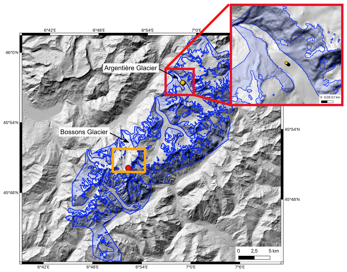
Figure 1Study area of the Mont-Blanc Massif. The static areas used to estimate the seasonal bias are represented in transparent blue. The Arg1 GNSS station on the Argentière Glacier tongue is represented with yellow dots (the station moved ∼130 m over the 3-year period). The area covered by Fig. S9 is represented by a yellow rectangle. The point considered in Fig. 7 is represented in red. It is located at (6.86759° E, 45.83930° N) over the accumulation area of the Bossons Glacier. The projection of the map is EPSG:32632, and the displayed coordinates are in EPSG:4326.
2.1 The Mont-Blanc Massif
We selected the Mont-Blanc Massif in the French Alps as our test site. The general orientation of the main ridge of this mountain range is southwest–northeast (Fig. 1). Most glaciers are steep and crevassed with low to moderate average surface flow velocities (tens to a few hundred meters per year). The valley floors surrounding the massif lie at low altitudes, ranging from approximately 1000 to 1500 m a.s.l., resulting in steep slopes with significant vertical elevation differences (up to ∼4000 m). Due to these characteristics, the Mont-Blanc Massif is often covered by shadows and is susceptible to significant illumination changes at the seasonal scale. In addition, several glaciers in the Mont-Blanc Massif have been monitored for half a century (Vincent et al., 2009; Six and Vincent, 2014; Vincent et al., 2022). In particular, continuous GNSS data have been acquired over the tongue of the Argentière Glacier for the period 2019–2021 (Vincent et al., 2022; Togaibekov et al., 2024, 2025). The Argentière Glacier extends from an altitude of 3400 to 1600 m a.s.l. at the glacier snout, and flows mainly towards the northwest (Fig. 1). This glacier, considered as the 19th largest glacier in the European Alps, has been widely studied using remote sensing and/or in-situ data (Roux et al., 2008; Fallourd et al., 2010; Vincent et al., 2022; Beraud et al., 2023; Rabatel et al., 2023; Roussel et al., 2025).
2.2 Remote sensing datasets
We use the following remote sensing velocity datasets that cover the Mont-Blanc Massif:
-
Monthly averaged velocity maps derived from Sentinel-2 images at a spatial sampling of 40 m by Troilo et al. (2024). Troilo et al. (2024) used the image correlation toolbox Glacier Image Velocimetry (GIV) (Van Wyk de Vries and Wickert, 2021). Monthly velocities are calculated as the weighted average of image-pair velocities (with temporal baselines ranging from 10 to 120 d) where the weights are proportional to the fraction of time included in a given month over the total time gap between the image-pairs. Previous filters are also applied: velocities higher than 1500 m yr−1 are discarded, and each image-pair velocity is smoothed using a 3×3 median filter. This dataset is later referred to as TRO.
-
Image-pair velocities derived from Sentinel-2 images with a modified version of the Normalized Cross-Correlation (NCC) algorithm ampcor from ROI_PAC (Mouginot et al., 2017; Millan et al., 2019, 2022; Mouginot et al., 2023). Here, we use two products with different levels of filtering to assess the impact of the filtering process. In the first product, velocities were filtered using a 9×9 median spatial filter only (hereafter referred to as “IGE with a spatial filter”). Unlike the other datasets, this product does not have a threshold to remove outliers with abnormally high velocities, and is not intended for release in its current form. The second product from IGE has undergone more advanced filtering (hereafter referred to as “IGE with advanced filters”), based on the maximal expected velocity magnitude, a range of temporal baselines selected based on the glacier flow magnitude vs. the expected accuracy, the flow direction, and the distribution of surface flow velocities, as described in Rabatel et al. (2023). Spatial sampling is 50 m and temporal baselines range from 5 to 400 d. The IGE products therefore allow us to assess the impact of seasonal biases at different levels of filtering, which is not possible for the other datasets, which are either already filtered and/or averaged through time.
-
Image-pair velocities from the NASA MEaSUREs project Inter-mission Time Series of Land Ice Velocity and Elevation (hereafter referred to as “ITS_LIVE with NDC filter”) dataset (Gardner et al., 2018, 2025). We only considered in this study velocities derived from optical satellites, i.e., Sentinel-2, Landsat-8 and 9 images. The displacement was measured using the NCC algorithm named “autoRIFT”. Outliers have been filtered out using the Normalized Displacement Coherence (NDC) (Gardner et al., 2018). This filter is applied to displacements divided by the NCC search distance. Displacements are accepted if seven or more of the values within a 5×5 pixel-centered window are within one-quarter of a search distance for both displacement components. Then, only displacements that agree within four times the centered mean absolute deviation are retained (Gardner et al., 2025). The spatial sampling of the velocity maps is 240 m resampled at a resolution of 120 m using a cubic spline approach. Temporal baselines range from 5 to 546 d.
A detailed comparison of these datasets is beyond the scope of this paper. Here, the objective is to investigate whether the seasonal biases are systematically present across different datasets.
Note that Sentinel-2 and Landsat-8/9 images are acquired at 10:30 a.m. and 10:00 a.m. Mean Local Solar Time (MLST), respectively, over the Mont-Blanc Massif (with a variation of ±10 min for Landsat-8/9).
2.3 GNSS data
We use data from the GNSS station ARG1 deployed along the glacier's central flowline between February 2019 and December 2021 (Togaibekov et al., 2024, 2025, 2026) (Fig. 1). The GNSS antenna was mounted on an aluminum mast anchored up to 6 m deep in the ice. GNSS data are processed in static mode using the high-precision geodetic software package GAMIT/GLOBK version 10.71 (Herring et al., 2018). The root-mean-square (RMS) scatter of the daily position estimates is about 2 mm in the horizontal directions (Fig. S1a–b in the Supplement), resulting in a horizontal velocity uncertainty of 2.3 mm d−1 (Fig. S1d). More details about the installation and processing can be found in Sect. S1 in the Supplement. We manually filtered out residual outliers and then computed a 30 d rolling mean for the antenna ARG1 to match the temporal sampling of remote sensing velocity time series extracted in Sect. 3.1, and focus only on the seasonal variations in Sect. 4.1. This step also reduces the uncertainty of the GNSS time series.
Below, we describe the methodology used in each of the section of the manuscript.
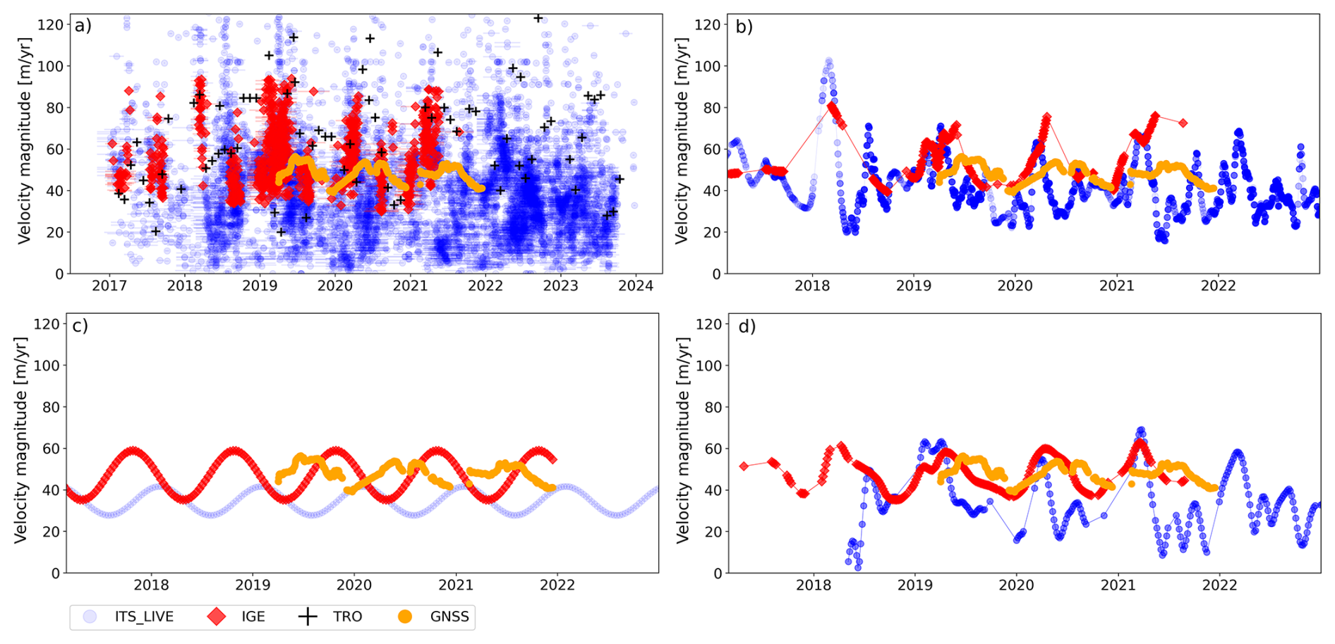
Figure 2Velocity magnitude at the location of the GNSS antenna installed on the tongue of Argentière Glacier (yellow dots in Fig. 1), measured using a 30 d rolling mean of the GNSS data in orange; and remote sensing datasets from “ITS_LIVE with NDC filter” in blue, “IGE with advanced filters” in red and “TRO” in black. (a) Raw velocity estimates from small baseline velocities (<180 d). Velocity post-processed using (b) LOWESS, (c) SR and (d) TICOI. Note that the maximum velocity magnitude of the ITS_LIVE and TRO datasets exceeds the limit of the axis in panel (a), reaching 400 and 500 m yr−1, respectively (see Fig. S2).
3.1 Evidence of seasonal biases highlighted by a comparison between remote sensing and GNSS data
To carry on a comparison between remote sensing and GNSS data, we first extract velocity time series from the remote sensing data, because remote sensing image-pair velocities with different temporal baselines are not comparable (Altena et al., 2019; Charrier et al., 2022) as they correspond to the average of the instantaneous velocity over the temporal baseline. To evaluate the sensitivity of the seasonal bias retrieval to the post-processing approach, we apply three state-of-the-art algorithms (Fig. 2): (1) LOcally WEighted Scatterplot Smoothing (LOWESS) (Derkacheva et al., 2021); (2) an integrated Sinusoidal Regression (SR, Greene et al., 2020); and (3) the Temporal Inversion using linear Combinations of Observations, and Interpolation (TICOI) package (Charrier et al., 2025). LOWESS is a nonparametric local regression that fits a weighted linear regression model to the k nearest neighbors. The weights are defined according to the distance between the center point and each of its neighbors. Derkacheva et al. (2021) recommend fitting 20 points. However, our datasets are noisier, therefore, we selected 70 points. The SR approach (Greene et al., 2020; Greene and Gardner, 2025) aims to de-trend the time series using weighted polynomial regression. It then integrates a simple sinusoid and applies it to displacement rather than velocity measurements. In this study, we only use the integrated SR, without de-trending the time series, because the inter-annual variations appear to be roughly constant between 2017 and 2023. Lastly, the TICOI approach fuses velocity measurements with different temporal baselines using the temporal closure principle (Charrier et al., 2022, 2025). We chose a regularization coefficient of 500, which was estimated by finding the inflection point of the averaged Velocity Vector Coherence calculated at several places in the entire massif for different values of regularization, as described in Charrier et al. (2025). Note that LOWESS must be applied to short temporal baseline velocities only (here, lower than 180 d), while the two other approaches can fuse velocities with different temporal baselines. However, we chose to exclude long temporal baselines (>180 d) from the dataset “ITS_LIVE with NDC filter” due to the strong temporal decorrelation (Fig. S2b).
3.2 Characteristics of seasonal biases inferred from static area analysis
In order to investigate the spatial and temporal characteristics of seasonal biases, we analyze the seasonal amplitudes and peak timings of image-pair velocities retrieved in static areas for different ranges of slopes and aspects.
3.2.1 Definition of static areas
Static areas are defined by excluding all areas within the glacier outlines from the Randolph Glacier Inventory v.7 (RGI Consortium, 2023), rock glacier inventories (Marcer et al., 2017) and active gravitational mass movements detected by InSAR as described in Sect. S2 (see blue polygons in Fig. 1).
3.2.2 Estimation of seasonal amplitudes and peak timings
Seasonal amplitudes and peak timings are estimated from time series smoothed using a weighted rolling circular median applied to the image-pair velocities stacked according to their respective day of the year. The window size of the rolling median is 30 d. The weights of the rolling median are defined using an exponential decay based on the temporal baselines: , with Δt the temporal baseline and L an empirical value set to 90 to provide higher weights to shorter temporal baselines (which are closer to the instantaneous velocity). Then, the amplitude is defined as the difference between the maximum and minimum of this smoothed time series, while the seasonal peak timing corresponds to the date of the maximum velocity. We choose this approach to retrieve the seasonal amplitude and peak timings from the raw datasets, without risking the addition of artifacts due to advanced post-processing methods such as LOWESS, SR or TICOI. Examples of smoothed time series and corresponding seasonal amplitudes and peak timings are illustrated in Fig. S12).
Note that the seasonal amplitudes of velocity magnitude are not estimated by applying this approach directly on the velocity magnitude time series. Velocity magnitudes follow a Rice distribution which could lead to an overestimation of the seasonal bias (Dehecq et al., 2019). To mitigate this effect, we estimate the seasonal amplitude of the velocity magnitude as:
with and the seasonal amplitudes estimated on the east/west and north/south velocity components, respectively. Seasonal peak timings are computed on the velocity magnitude because the sign of velocity components depends on the direction of the velocity vector.
3.2.3 Comparison with slopes and aspects
To characterize the spatial pattern of seasonal biases, we compute the median amplitudes and peak timings for every 10° bin of slopes and aspects. These parameters are derived from the Copernicus 30 m DEM (ESA, 2024) using the xdem library (xDEM contributors, 2024).
3.3 Potential origins of seasonal biases
3.3.1 Number of days under shadow extent and edges
To map areas affected by shadow casting, we simulate shadows projected by the Copernicus 30 m DEM (ESA, 2024) every day at 10:30 MLST, corresponding to the acquisition time of Sentinel-2 images; Copernicus Sentinels, 2015), for one arbitrary year (here 2024). For this, we use the package horayzon which takes hours in UTC as input (Steger et al., 2022). Therefore, we converted MLST to UTC using a longitude correction: 10:30 MLST corresponds to 10:02 UTC. Then, we compute for every pixel the number of days under shadow extent in 2024. In addition, we estimate the number of days under shadow edges. For that, we compute the difference between a dilation and an erosion, carried out using a disk of radius 160 m, for every daily shadow map. We chose 160 m to match the dimension of the correlation window used in the IGE dataset, which is 16 pixels, corresponding to 160 m on Sentinel-2 images.
3.3.2 Plane of array irradiance, a proxy of illumination changes
To estimate the changes in illumination, we derive the Plane Of Array (POA) irradiance. It corresponds to the total amount of light received by a square meter on a tilted panel. In addition to direct irradiance, the tilted panel receives diffuse and reflected irradiance. The POA irradiance depends on the sun azimuth and elevation, the panel angle, the soil reflectance factor, and other parameters. We simulated the POA irradiance using the pvlib package (Anderson et al., 2023). First, we compute the sun position at 10:00 UTC for every day in 2024. Then, we derive the clear-sky irradiance using the Ineichen and Perez clear-sky model, which is implemented by default. The geometry of the tilted panel is defined by the slope and aspect of each pixel, estimated from the Copernicus 30 m DEM (ESA, 2024) using the xdem library (xDEM contributors, 2024). Finally, we compute the average and Coefficient of Variation (CV) of POA irradiance for the year 2024. The CV corresponds to the ratio of the standard deviation to the mean.
3.4 Mapping of areas affected by seasonal biases
To mitigate the effect of seasonal biases, we implement a strategy to identify their location and amplitude.
First, we propose automatically mapping areas affected by shadow casting. We consider a given pixel to be significantly affected by shadow casting if it is under shadow edges more than 30 d, as simulated in Sect. 3.3.1.
Second, we estimate the expected seasonal biases over glacier areas. For this, we rely on the derived seasonal amplitude over static areas (Sect. 3.2). We compute the median of the distribution for each quadrant (northwest, northeast, southwest, southeast) for bins of 30° slope, to minimize the effect of an inaccurate DEM. The estimated amplitude is then interpolated for all glacier surfaces based on the corresponding slope and aspect of each pixel. Note that we could use the POA irradiance for this estimation, but this would take more computation time.
4.1 Evidence of seasonal biases highlighted by a comparison between remote sensing and GNSS data
Remote sensing velocities are compared with GNSS data over the tongue of Argentière Glacier at the ARG1 location (Fig. 1), to investigate the accuracy of the seasonality recovered using remote sensing. GNSS data show a mean horizontal velocity of 48 m yr−1, with a seasonal amplitude (defined as the difference between the yearly maximum and minimum) of 15 m yr−1 and a velocity peak timing in May/June.
The raw remote sensing datasets show a large dispersion (Fig. 2). The average velocity magnitudes between 2017 and 2024 are 45, 57 and 74 m yr−1 for the datasets “ITS_LIVE with NDC filter”, “IGE with a spatial filter” and “TRO” respectively. The standard deviation is about 30, 10 and 54 m yr−1 respectively. Maximum values reach up to 400 and 500 m yr−1 for “ITS_LIVE with NDC filter” and “TRO” respectively (Fig. S2). This may be due to noise, and heterogeneous temporal baselines for the datasets “IGE with advanced filters” (Rabatel et al., 2023) and “ITS_LIVE with NDC filter” (Fig. 2a). Therefore, it requires post-processing these two datasets to estimate velocity time series before investigating seasonal changes. To evaluate the sensitivity of the seasonality amplitude/phase retrieval to the post-processing approach, we applied three state-of-the-art strategies defined in Sect. 3.1. The TRO dataset (Troilo et al., 2024), available in open-access, already corresponds to monthly velocity time series.
The average amplitude during the 2019–2021 period measured using LOWESS, SR and TICOI post-processing is 29, 23 and 20 m yr−1 for the dataset “IGE with advanced filters”; 43, 14 and 40 m yr−1 for the dataset “ITS_LIVE with NDC filter”, respectively. This highlights that remote sensing products overestimate the amplitude by up to a factor of three and by 90 % on average. Moreover, this underlines the dispersion of the retrieved amplitude, especially for the dataset “ITS_LIVE with NDC filter” which is less filtered and noisier over this area. The peaks in velocity observed after applying the LOWESS, SR and TICOI approaches are located in April–June (LOWESS), October (SR) and April (TICOI) for the dataset “IGE with advanced filters”; April (LOWESS), February (SR) and April (TICOI) for the dataset “ITS_LIVE with NDC filter”. The peak timing variability observed when applying LOWESS to the dataset “IGE with advanced filters” is probably due to the scarcity of small baseline image-pair velocities. The combination of long and small baseline velocities alleviates this problem (Fig. 2d). We observe that SR provides the closest seasonal amplitude to the GNSS signal; however, the timing of the peaks is located four months later than the expected peak for the dataset “IGE with advanced filters”, and four months earlier for the dataset “ITS_LIVE with NDC filter”. We note that no clear seasonality appears in the TRO monthly velocity time series over this point.
It is worth mentioning that the SR approach differs from that used to produce ITS_LIVE seasonal maps (Greene et al., 2020): no previous filtering or detrending is applied in our case and the regression is carried out over a shorter time range. It is also worth noting that surface flow velocities on this part of the Argentière Glacier are difficult to map at a seasonal scale, due to a relatively low glacier surface velocity (<60 m yr−1), which does not provide a favorable signal-to-noise ratio for short repeat cycles (Millan et al., 2019). This analysis is not representative of the performance of each dataset and method. A proper comparison would require a dedicated study involving several benchmarks and a sensitivity analysis. Nevertheless, this analysis highlights a systematic overestimation of the seasonal amplitude across different datasets regardless of the post-processing strategy used. We therefore extend the analysis to static areas over the Mont-Blanc Massif to assess whether our findings on Argentière Glacier are systematic.
4.2 Characteristics of seasonal biases inferred from static area analysis
To assess the characteristics of seasonal biases, we examine the seasonality of velocity in areas assumed to be static, as defined in Sect. 3.2. We consider both the seasonal amplitudes and peak timings which are extracted as described in Sect. 3.2. Seasonal amplitudes correspond to the difference between the maximum and minimum velocity over one year while seasonal peak timings represent the day of the year when the maximum velocity occurs.
4.2.1 Seasonal amplitudes
The highest seasonal amplitudes are observed on north-facing slopes, and especially on northwest-facing slopes with steep slope angles (Figs. 3 and 4). This is consistently observed for both the ITS_LIVE and IGE datasets, for different levels of filtering (Figs. S4 and S5). This highlights the systematic nature of seasonal biases. These results are consistent with Lacroix et al. (2019) and Mueting et al. (2026) who conducted a similar analysis on landslides in Peru and Argentina, respectively. Both studies reported the highest amplitudes on south-facing slopes, which are equivalent to the north-facing slopes in the Southern Hemisphere.
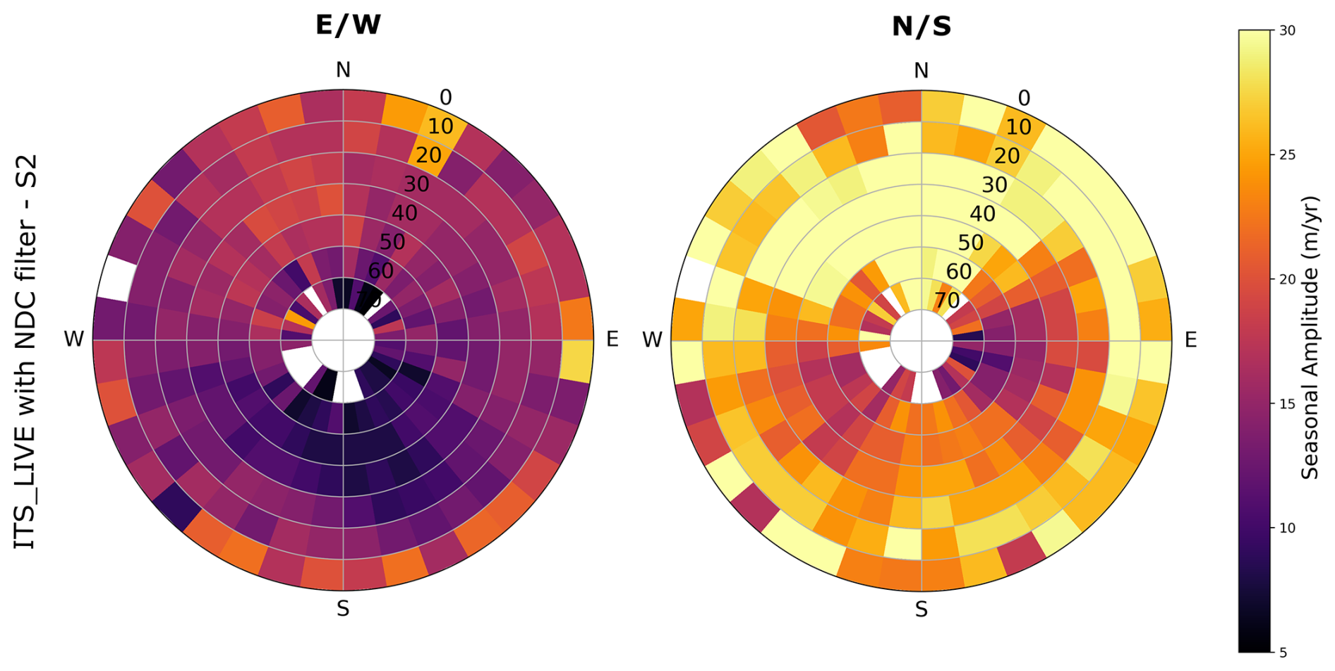
Figure 3Polar diagram of the median seasonal amplitude of east/west (left) and north/south (right) velocity components of the dataset “ITS_LIVE with NDC filter” using Sentinel-2 images only, over static areas. The size of the bin is 10° for both slope and aspect. The slopes are shown along the radial axis, with the highest slopes in the center.
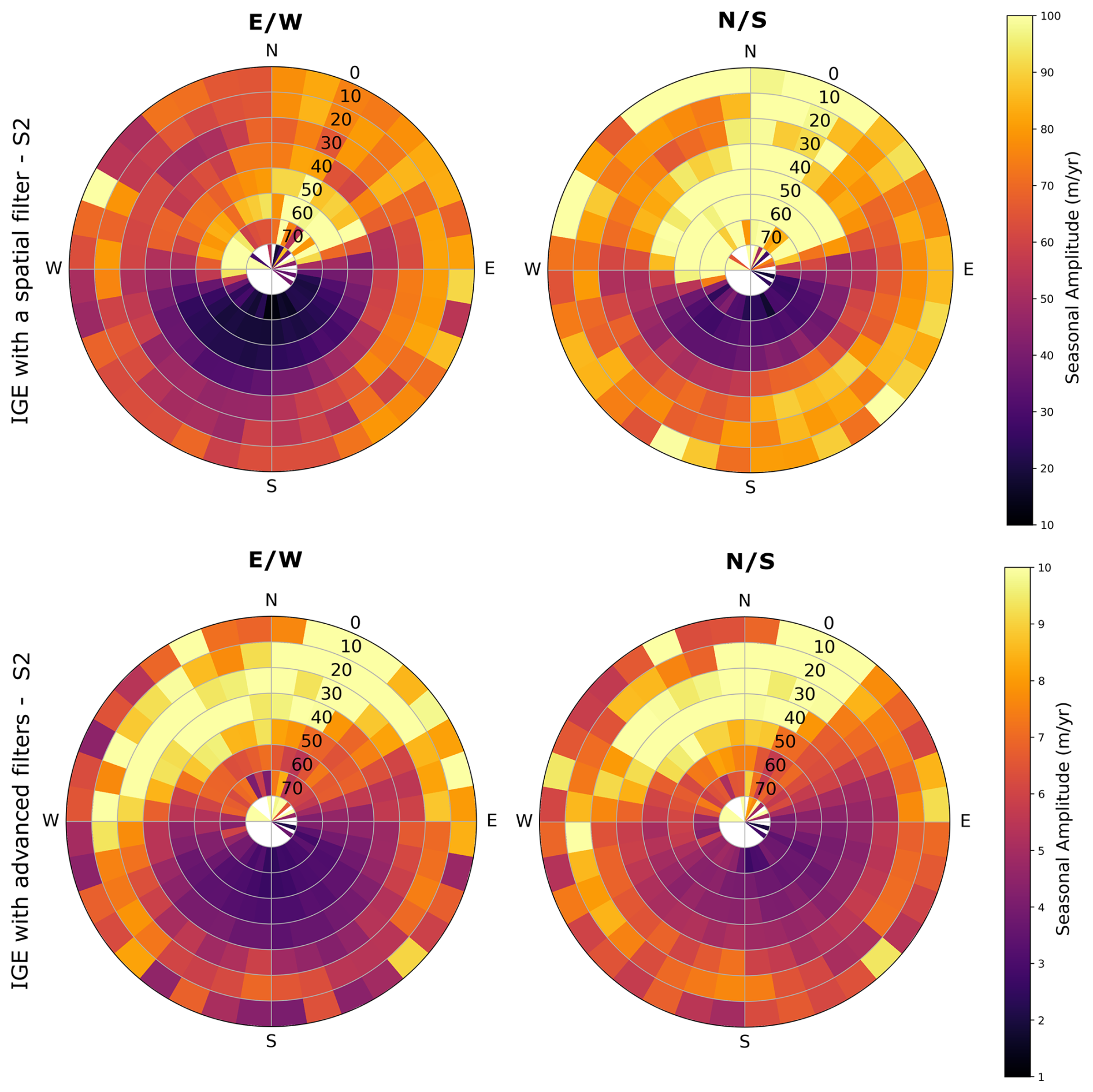
Figure 4Polar diagram of the median seasonal amplitude of east/west (left) and north/south (right) velocity components of the datasets “IGE with advanced filters” and “IGE with a spatial filter only” (top and bottom rows) over static areas. The size of the bin is 10° for both slope and aspect. The slopes are shown along the radial axis, with the highest slopes in the center. Note that the color bars have different ranges.
The median and 90th percentile of the amplitude in static areas for north-facing slopes are:
-
16 and 29 m yr−1 (east/west components) and 28 and 54 m yr−1 (north/south components) for the dataset “ITS_LIVE with NDC filter” based on Sentinel-2 images (Figs. S4 and 3)
-
29 and 55 m yr−1 (east/west components) and 47 and 88 m yr−1 (north/south components) for the dataset “ITS_LIVE with NDC filter” based on Landsat-8,9 images (Figs. S4 and S3)
-
71 and 308 m yr−1 (east/west components) and 93 and 428 m yr−1 (north/south component) for the dataset “IGE with a spatial filter only” (Figs. S5 and 4). The high percentile values, compared to the other datasets, can notably be explained by the fact that this dataset has been filtered using a spatial filter only.
-
8 and 38 m yr−1 (east/west components) and 7 and 33 m yr−1 (north/south component) for the dataset “IGE with advanced filters” (Figs. S5 and 4).
First, we notice that seasonal biases depend on the satellite missions used to derive the velocities. The amplitude tends to be higher with ITS_LIVE velocities based on Landsat-8,9 images than with those based on Sentinel-2 only. The median amplitude is multiplied by 1.6 and 1.8 for the east/west and north/south components, respectively, on north-facing slopes. This difference may be explained by different spatial and radiometric resolutions and slightly different acquisition times between Landsat-8,9 and Sentinel-2.
Second, these results highlight the impact of the filters used to reject outliers. The amplitude of the seasonal bias drastically decreases with the use of advanced filters in the IGE dataset (which are based on the maximal velocity magnitude, the temporal baseline, the flow direction, and the distribution of surface flow velocities, as described in Sect. 2). We also note that the differences between the east/west and north/south components are reduced. This underlines the importance of filtering surface velocity fields derived from optical image correlation, especially with direction-based criteria. However, even in a dataset where a wide range of filters has been applied, seasonal biases persist: for north-facing slopes, we observe a median of 7 m yr−1 and 90th percentile of 30 m yr−1 (Fig. S5).
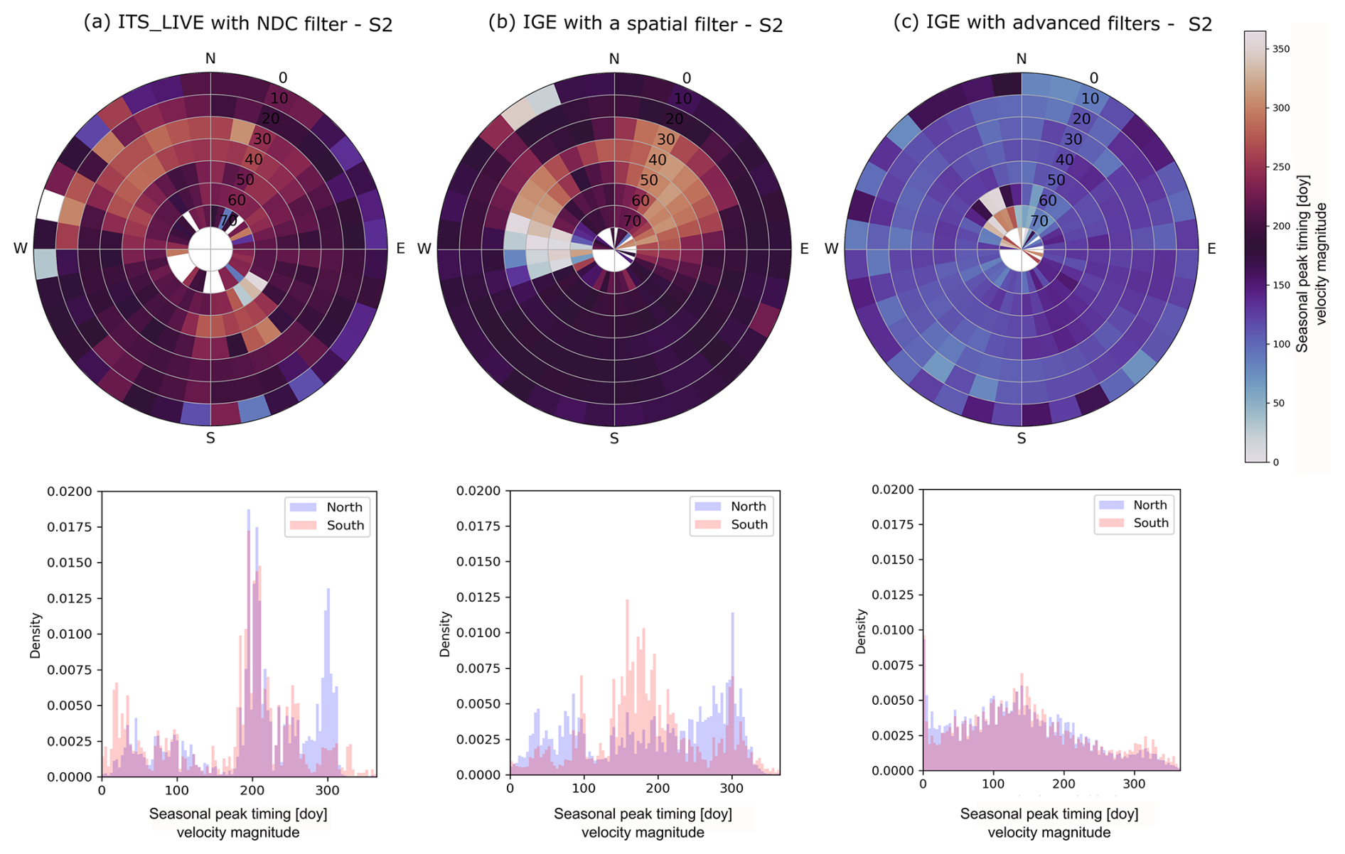
Figure 5Polar diagram (top) and histogram (bottom) of the seasonal peak timings of velocity magnitude over static areas for the datasets: (a) “ITS_LIVE with NDC filter” using Sentinel-2 images (left column), (b) “IGE with a spatial filter”, and (c) “IGE with advanced filters”. In the polar diagram, the circular mean is computed for each 10° bin of slope and aspect, with slopes represented along the radial axis (highest slopes at the center).
4.2.2 Seasonal peak timings
Seasonal peak timings (i.e., the date of the maximum seasonal velocity; see Sect. 3.2) retrieved over static areas are also significantly different between south- and north-facing slopes (Fig. 5). We draw three key observations.
First, for both the datasets “ITS_LIVE with NDC filter” and “IGE with a spatial filter only”, we observe that seasonal peak timings occur between days 260 and 330 of the year (i.e., between August and October) on north-facing slopes, especially for the steepest slopes (Fig. 5a and b). This peak timing is centered on the autumn equinox in the Northern Hemisphere. On south-facing slopes, the seasonal velocities reach a maximum mainly around days 180 and 240 of the year (i.e., between June and August).
Second, for the dataset “IGE with a spatial filter only”, we also notice another high-density seasonal peak timing on north-facing slopes around day 90 of the year, corresponding to the spring equinox (Fig. 5b). This is especially observed on northwest-facing slopes, for the steepest slopes.
Third, for the dataset “IGE with advanced filters” the seasonal peak timings show no significant differences between south- and north-facing slopes (Fig. 5c). This further highlights the ability of the filters to reject outliers.
The analysis of both seasonal amplitudes and peaks over static areas reveals a systematic seasonal bias over the Mont-Blanc Massif. To better characterize it, we examine potential sources of bias and the characteristic patterns they may produce in the following section.
4.3 Potential origins of seasonal biases
Seasonal biases exhibit strong spatial variations. These variations can result from several phenomena:
-
The casting of shadows by the topography and the local relief (crevasses, seracs, etc.). Seasonal biases will especially arise when image correlation algorithms track the edges of the shadows.
-
Changes in image contrast due to variations in illumination and surface properties.
4.3.1 Cast shadow effect
To investigate the cast shadow effect, we simulate the number of days under shadow extent and edges (see Sect. 3.3.1). We observe these numbers to be larger on northwest-facing slopes (Fig. S7) because shadows are elongated towards this direction in the Northern Hemisphere at the time of Sentinel-2 satellite acquisitions (the sun azimuth position is about 151° at the winter solstice over the Mont-Blanc Massif). Note that shadows would be elongated towards the southwest in the Southern Hemisphere. We observe a clear correlation between the velocity amplitude in static areas and the number of days under shadow extent or edges, except for topographic ridges (Fig. 6).
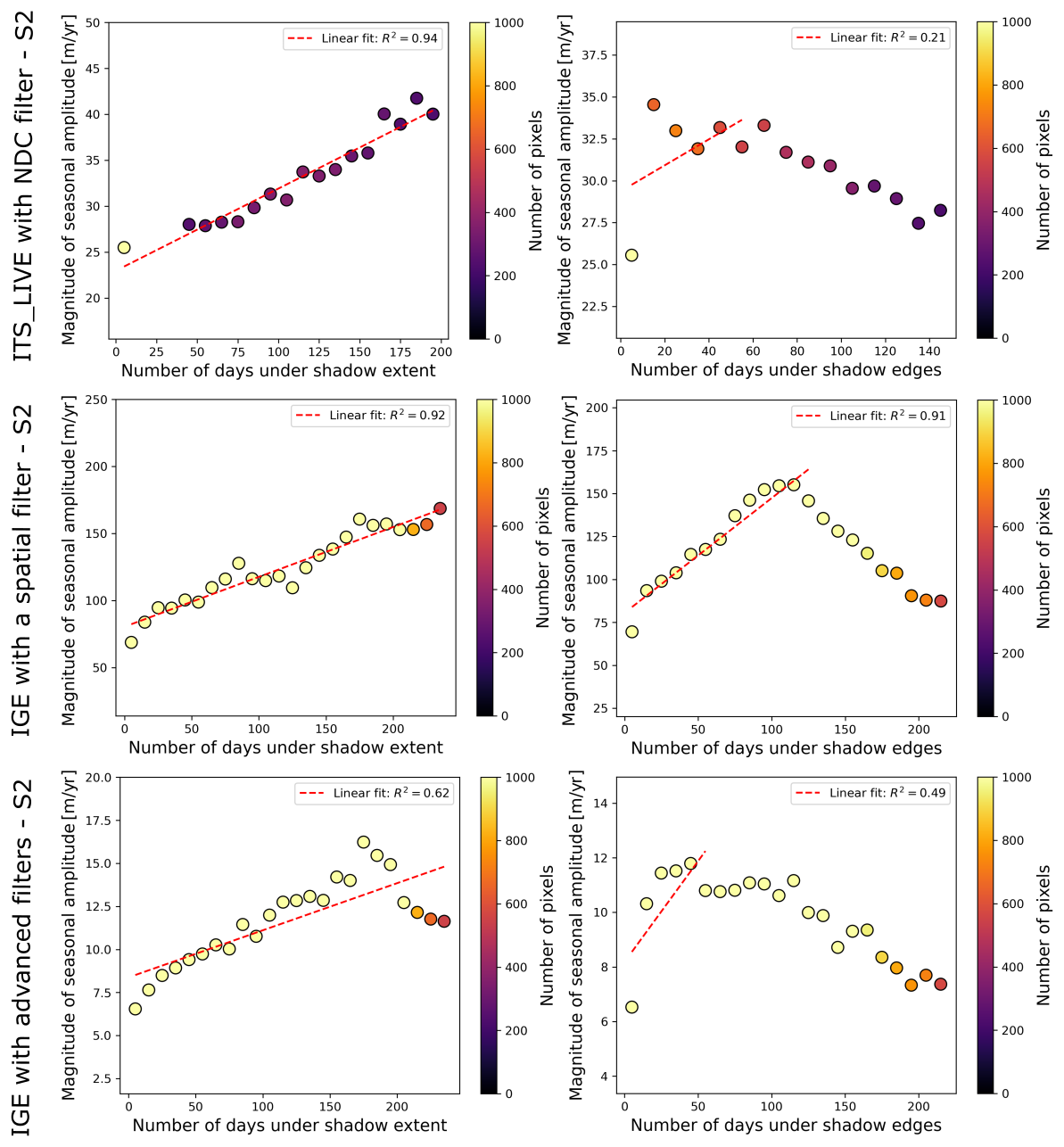
Figure 6Magnitude of seasonal velocity amplitudes retrieved in static areas as a function of the number of days under shadow extent (left) and edges (right). Each dot corresponds to the median magnitude of seasonal velocity amplitudes binned by 10 d under shadow extent or edges. A linear trend (represented by a dashed red line) is observed when the number of pixels is sufficient. Bins where the number of days under shadow edges exceeds than 120 d correspond to topographic ridges; the linear correlation does not hold in these areas. Note that bins where the number of pixels is insufficient are filtered out (corresponding to 500 pixels for the datasets “IGE with a spatial filter” and “IGE with advanced filters”, and 200 for the dataset “ITS_LIVE with NDC filter”). The number of points is lower for the dataset “ITS_LIVE with NDC filter” than for the datasets “IGE with advanced filters” and “IGE with a spatial filter”, because the spatial sampling is 120 m for the first dataset and 50 m for the other two datasets.
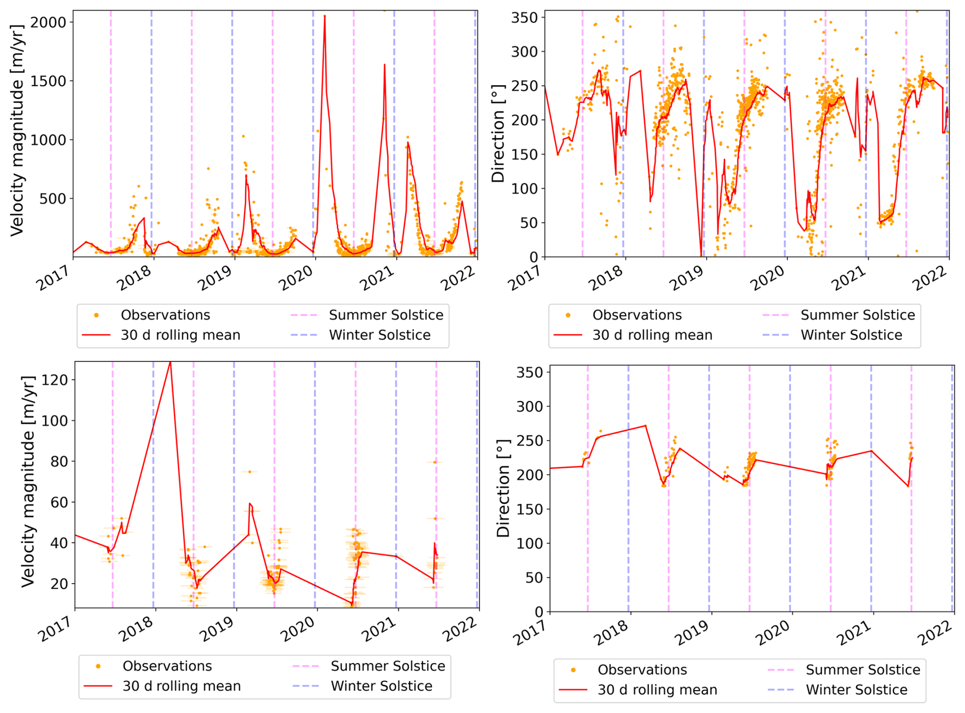
Figure 7Example of velocities capturing shadow casting at the point located at (6.86759° E, 45.83930° N) (red dot in Figs. 1, S6 and S9), over the accumulation area of Bossons Glacier. The upper panel corresponds to the dataset “IGE with a spatial filter” and the lower panel corresponds to the dataset “IGE with advanced filters”. Velocity magnitudes are displayed in the left column, and directions in the right column. Shadow casting is illustrated on two Sentinel-2 images in Fig. S9.
A typical shadow casting example can be observed at the coordinate (6.86759° E, 45.83930° N), located in the accumulation part of the Bossons Glacier (Fig. S9). The flow direction deviates towards the west in autumn and towards the east in spring (Fig. 7). The velocity magnitude rises from the winter solstice to the spring equinox and decreases afterwards until the summer solstice (Fig. 7). The same cycle is repeated between the summer and winter solstices. This pattern corresponds to the casting of a shadow projected by the local relief, as illustrated by a drawing in Fig. S8, and on optical images in Fig. S9. This pattern is consistent with our observations over static areas: the seasonal bias induced by shadow casting tends to be maximal at the spring and autumn equinoxes. We note that filtering velocities, especially by removing velocities that deviate more than 45° from the average velocity, cuts the seasonal fluctuations and keeps only the lower part of the distribution (Fig. 7). However, these fluctuations may still reflect shadow casting and rather than real glacier displacements.
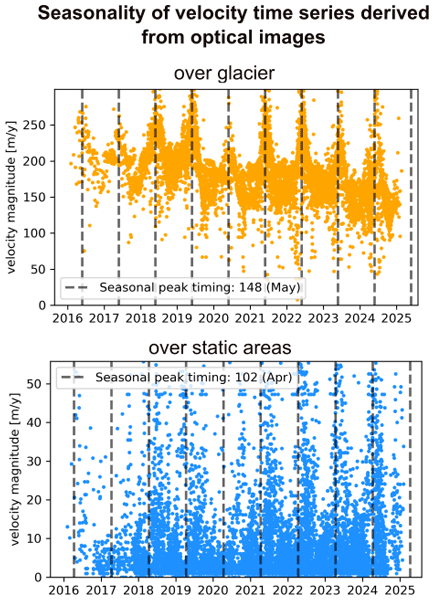
4.3.2 Illumination changes effect
To estimate the effect of illumination changes, we derive the average and CV of the POA irradiance (see Sect. 3.3.2). The average and Coefficient of Variation (CV) of POA irradiance are, respectively, lower and higher for north- compared to south-facing slopes (Fig. S10). In addition, the CV is higher for north-facing slopes with angles between 20 and 60°. This is similar to the pattern observed in velocity amplitudes over static areas, especially for the datasets “ITS_LIVE with NDC filter” and “IGE with a spatial filter”.
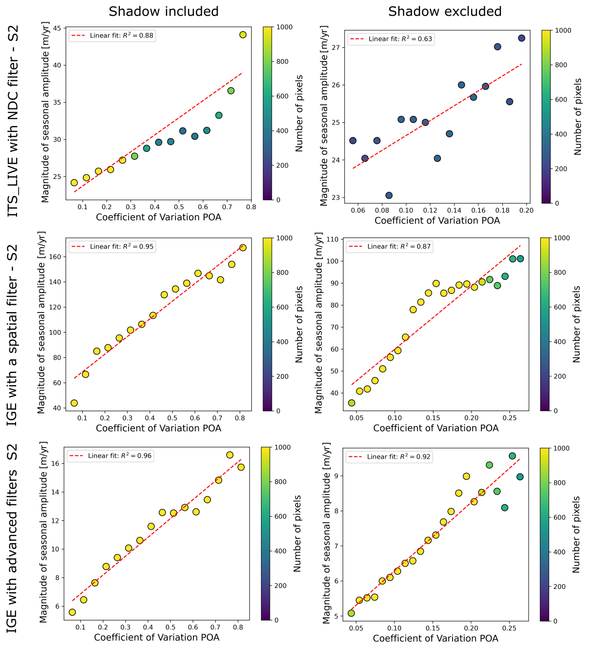
Figure 8Magnitude of seasonal velocity amplitudes retrieved over static areas as a function of the Coefficient of Variation (CV) of POA irradiance when shadows are included (left) and excluded (right), for the datasets “ITS_LIVE with NDC filter” (top), “IGE with a spatial filter” (middle) and “IGE with advanced filters” (bottom). Each dot corresponds to the median magnitude of seasonal velocity amplitudes over a bin of 0.05. Bins where the number of pixels is unsufficient enough are filtered out (corresponding to 500 pixels for the datasets “IGE with a spatial filter” and “IGE with advanced filters”, and 200 for the dataset “ITS_LIVE with NDC filter”).
A linear correlation between the CV of POA and the amplitude of the velocity magnitude in static areas is observed for the three datasets in Fig. 8 (R2 score range between 0.88 and 0.96). Because the POA pattern follows the same pattern as shadows, we exclude areas with at least 1 d under shadow extent. The linear relationship remains (with a R2 score of 0.63 and 0.92).
Therefore, we conclude that both cast shadow and illumination changes control seasonal biases. They are related since shadow casting is likely to be observed on north-facing slope in the Northern Hemisphere, areas for which the illumination changes are the strongest (Figs. S7 and S10). However, shadow casting does not only depend on the slope and aspect of the given pixel; it depends mainly on the topography above. Hence, both shadow casting and illumination changes should be considered.
4.3.3 Other potential sources of seasonal biases
It is worth mentioning that other effects may play a role:
-
changes in the surface state between the two images of a pair (e.g., snow on one image and ice on the other, snow melt occurring between the two images). However, high surface changes usually result in completely incoherent velocities, which can be filtered out using the correlation score or spatio-temporal filters. In addition, seasonal biases caused by changes in illumination and shadow casting have also been observed in areas without any snow cover, such as in desert or semi-arid climates (Lacroix et al., 2019; Ding et al., 2020; Mueting et al., 2026).
-
an imbalance in the temporal density of available images between summer and winter is also susceptible to resulting in an erroneous seasonality, but we did not observe such an effect in our study area.
-
geometric refinement of the DEM used to co-register the optical images may also play a role, as described by Provost (2025). They noticed strong seasonal displacement over the Aletsch Glacier before summer 2021, and much smaller displacements afterwards for the same pixel. This may be due to a geometric refinement with the Copernicus DEM after summer 2021. Even though we did not see this effect for the ITS_LIVE and IGE datasets over the static areas of the Mont-Blanc Massif (Fig. S11), or as a general trend in the glacier covered areas, this effect could still impact some datasets and study areas and needs to be considered.
4.4 Towards a map of areas affected by seasonal biases
We propose a strategy to identify areas affected by shadows and illumination changes in two steps: (1) mapping of areas affected by shadow casting and (2) estimating seasonal biases over glacier areas (Sect. 3.4). The methodology is implemented in a Python package called SeBVel for Seasonal Biases in Velocity measurements.
First, SeBVel enables the user to automatically map shadows because this is not straightforward to do manually. For example, some areas affected by shadow casting, such as the upper part of the Bossons Glacier or the Combe Maudite in the accumulation zone of the Mer de Glace (red point and green rectangle, respectively, in Fig. S6) were not excluded from the study of Troilo et al. (2024), despite manual mapping of areas affected by shadow casting. Here, we propose a code to simulate the number of days under shadow extent and edges according to a given DEM (Sect. 3.4). Areas with a large number of days can be masked out before analyzing seasonal velocity time series to avoid artifacts (Fig. 9).
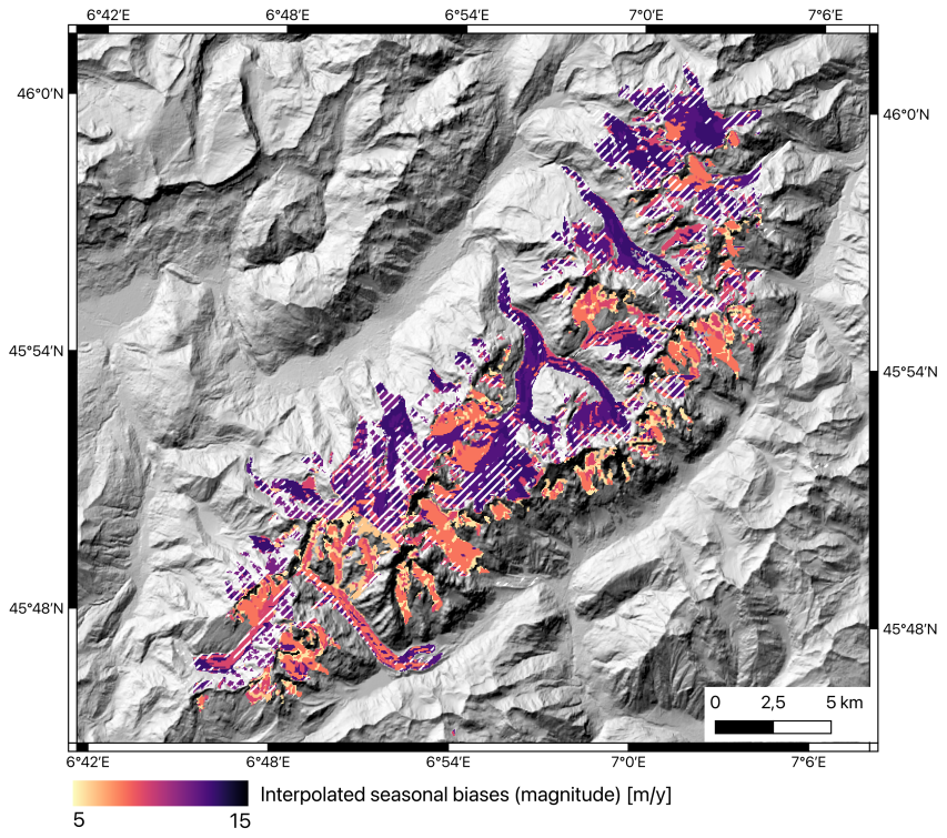
Figure 9Estimated location and amplitude of seasonal biases over the Mont-Blanc Massif. Areas affected by shadow casting (number of days under shadow edges higher than 30), and assumed to be unreliable for seasonal analysis, are represented by hashed white lines. The amplitude of the expected seasonal bias based on an analysis of static areas for the “IGE with advanced filters” dataset is shown in color scale. The background corresponds to a hillshade from the Copernicus 30 m DEM (ESA, 2024). The projection of the map is EPSG:32632 and the displayed coordinates are in EPSG:4326.
Second, we propose estimating the amplitude of the expected seasonal bias, based on an analysis of static areas with similar slopes and aspects (Sect. 3.4). For the dataset “IGE with advanced filters”, the bias in velocity amplitude is estimated to be about 12 m yr−1 over the tongue of the Argentière Glacier, which is consistent with the error in velocity amplitude obtained while comparing this dataset with the GNSS data in Sect. 4.1. The average estimated seasonal bias for the entire Mont-Blanc Massif is 10 m yr−1. Such a map can ultimately be used to assess whether the retrieved seasonal variations are significant compared to the seasonal bias and if they could be attributed to actual ice velocity fluctuations. This approach could be employed for different datasets, post-processed with different strategies.
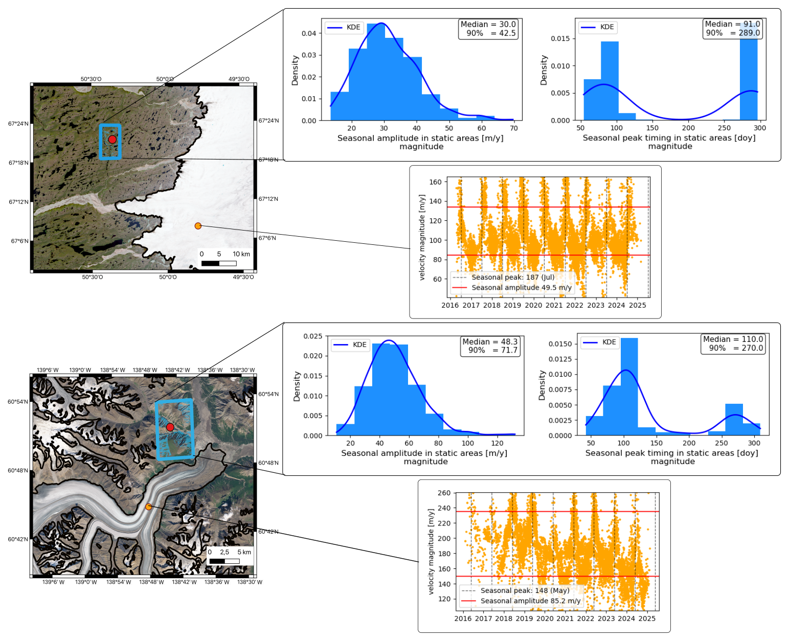
Figure 10Example of seasonal biases identified by comparing seasonal velocity amplitudes and peak timings over static areas (blue histograms) and moving areas (orange dot) for the Issungata Sermia Glacier in Western Greenland (top) and Kaskawulsh Glacier in Yukon, Canada (bottom). The time series in moving areas correspond to raw ITS_LIVE image-pair velocity magnitude acquired at the location of the orange dots represented on the left. The histograms over static areas correspond to the seasonal amplitudes and peak timings derived as described in Sect. 3.2 over static areas with the same range of aspects and slopes as the moving point, i.e., a slope between 0 to 30° for both sites, an aspect between 180 and 270° for Issungata Sermia and 0 and 90° for Kaskawulsh. These areas are represented by blue polygons inside the blue rectangles. Black lines correspond to the ice-sheet or glacier contourlines defined in the PROMICE (Luetzenburg et al., 2025, 2026) or RGI (RGI Consortium, 2023) databases. Backgrounds are Sentinel-2 images in UTM projection. KDE stands for Kernel Density Estimation.
5.1 Evidence of seasonal biases in different regions worldwide
We chose the Mont-Blanc Massif to analyze seasonal biases because of the availability of GNSS data and different velocity products. However, seasonal biases are observed over glaciers and ice sheets worldwide. Seasonal biases mainly depend on the local topography and the sun incidence angle. We illustrate other examples of seasonal biases in Western Greenland, near the terminus of Issungata Sermia and in Yukon, Canada, near the tongue of the Kaskawulsh Glacier (Fig. 10). We apply the same methodology described in Sect. 3.3.1 to ITS_LIVE image-pair velocities to infer seasonal velocity amplitudes and peak timings over both static and glacier areas. Over the glaciers, velocity peaks in July and May with an amplitude of 50 and 85 m yr−1, respectively, for Issungata Sermia and Kaskawulsh Glaciers. This has to be compared with the amplitude retrieved in static areas where clear seasonal patterns are observed (see the examples over two particular points in Fig. S12. To obtain a robust estimation of seasonal amplitudes and peak timings, we consider static areas with similar slopes and aspects to the moving point (blue polygons in Fig. 10). Over these areas, velocity peaks in spring and/or autumn for both sites, with a median amplitude between 30 and 48 m yr−1 for Issungata Sermia and Kaskawulsh Glaciers respectively. This is not negligible, as it represents 60 % and 50 % of the observed amplitude for Issungata Sermia and Kaskawulsh Glaciers, respectively.
This analysis is also consistent with the trend in velocity magnitude errors obtained by comparing ITS_LIVE image-pair velocities to GNSS velocities over the tongue of the Kaskawulsh Glacier (Lower GNSS station in Charrier et al., 2025; Van Wychen et al., 2023; Waechter et al., 2015) (Fig. S13). The errors follow a seasonal pattern with two maxima. The first maximum is reached in spring, between days 120 and 160 of the year while the second maximum is reached in autumn, between days 250 and 300 of the year.
The amplitudes of seasonal biases reported here are not negligible, but could be reduced by post-processing the image-pair velocities before estimating seasonal amplitudes.
5.2 Possible other strategies to reduce seasonal biases
In this study, we propose a framework to estimate the location and amplitude of seasonal biases. We emphasize the importance of a drastic filtering of the image-pair velocities to reduce the amplitude of these biases. However, other strategies can also be considered to mitigate seasonal biases during the post-processing of image-pair velocities, particularly through a post-processing approach based on temporal closure inversion, as described in Bontemps et al. (2018), Lacroix et al. (2019), Ding et al. (2020), Charrier et al. (2025). Recently, Mueting et al. (2026) compared different strategies proposed for studying dunes and landslides:
-
removing a seasonal error, estimated on static areas through harmonic functions, from the displacement time series (Lacroix et al., 2019);
-
restricting the image-pair velocities used as input of the temporal closure inversion to pairs with similar illumination (Ding et al., 2020);
-
weighting the temporal closure inversion using a proxy of illumination changes (Bontemps et al., 2018);
-
upsampling optical images (Antoine and Liu, 2025).
They found strategy (2) to be the most efficient. The study site of Mueting et al. (2026) is a slow-moving landslide in northwest Argentina. However, the same strategies could be used for glaciers because the effects of shadows and illumination changes are not object-dependent.
Despite the growing interest in quantifying sub-annual variability in glacier velocity, no study has systematically analyzed seasonally correlated biases, which can affect the interpretation of short-term ice flow variability. This is especially critical when investigating glacier velocities that have a seasonal cycle with an amplitude of a few to hundred m yr−1, which encompasses the majority of mountain glaciers and the interiors of ice sheets.
Here, we demonstrate that sub-annual velocity measurements derived from optical satellite images are influenced by seasonally correlated biases. Remote sensing velocities systematically overestimate seasonal amplitudes in comparison to GNSS data, regardless of the filtering and regression approach used to post-process the image-pair velocities. Based on an analysis over static areas, we estimate that these biases are primarily concentrated on north-facing slopes in the Northern Hemisphere (and south-facing slopes in Southern Hemisphere) and are driven by shadow casting and irradiance variations. The magnitude of this bias depends on the satellites used to derive glacier surface velocities and the filters applied to remove outliers. For our study area of the Mont-Blanc Massif, the median value of these seasonal biases for north-facing slopes are about 10, 20 and 80 m yr−1 (for strong to low levels of filtering). The 90th percentile is about 30, 40 and 400 m yr−1 (for strong to low levels of filtering). These biases are maximal around the spring and autumn equinoxes. Our results highlight that the use of a wide range of filters, based on the maximal velocity amplitude, the flow direction, the temporal baselines, or the velocity distribution, drastically reduces the amplitude of seasonal biases. However, the measured velocities could still reflect shadow tracking, rather than actual terrain motion, in areas affected by shadow casting.
This effect is not specific to the Mont-Blanc Massif and can be observed worldwide. We illustrate seasonal biases over two other sites: Kaskawulsh Glacier in Yukon, Canada and Issungata Sermia in Western Greenland. Therefore, it appears crucial to interpret sub-annual velocity variability after a careful post-processing of the raw image-pair velocities and an estimation of the seasonal biases, regardless of the region of interest. Otherwise, erroneous conclusions about seasonal variations in velocities can be drawn.
In this context, we propose a strategy to identify the location and amplitudes of seasonal biases by (1) automatically mapping areas affected by shadow casting and (2) estimating the amplitude of the bias in the remaining areas. First, we compute the number of days affected by shadow casting for each pixel of the velocity field, according to a simulation of shadow cast over a given DEM. We propose masking out areas where the number of days in cast shadows is too large (e.g., 30). Second, based on an analysis of static areas with similar slopes and aspects, we estimate the amplitude of the expected seasonal bias. The amplitude of the seasonal velocity retrieved over glaciers can be compared to this bias to assess the significance of the estimated seasonality. This approach can be easily applied to any area and dataset and is transferable to other displacement estimation applications, such as landslides or dunes.
This study provides a first guideline for accounting for seasonal biases in the interpretation of glacier sub-annual velocity time series. The code is released as a Python package called SeBVel for Seasonal Bias in Velocity measurements.
The code is available on https://doi.org/10.5281/zenodo.23923112 (Charrier, 2026a). The simulated number of days under shadow extent and edges, and the estimated error in the amplitude of velocity magnitude is available on https://doi.org/10.5281/zenodo.23420040 (Charrier, 2026b).
The supplement related to this article is available online at https://doi.org/10.5194/tc-20-6767-2026-supplement.
LC, FB, AR and AD designed the study. LC and NL worked on the python package with advice from AD, AR and FB. LC generated and analyzed the results with feedbacks from AD, FB, AR and RM. RM and AR derived the velocity field from IGE. AW and AT provided the GNSS data. DC provided an inventory of active moving areas detected from InSAR. LC led the writing, and all authors contributed to it.
The contact author has declared that none of the authors has any competing interests.
Publisher's note: Copernicus Publications remains neutral with regard to jurisdictional claims made in the text, published maps, institutional affiliations, or any other geographical representation in this paper. The authors bear the ultimate responsibility for providing appropriate place names. Views expressed in the text are those of the authors and do not necessarily reflect the views of the publisher.
LC and DC acknowledge support from the Centre National d'Etudes Spatiales for their respective postdoctoral fellowships. AD and LC acknowledge support from the French Programme National de Télédétection Spatiale (PNTS), project EDYGHMA. The GNSS data presented in this study have been acquired in the framework of the project SAUSSURE (PI Christian Vincent, IGE) supported by the Agence Nationale de la Recherche (contract ANR-18-CE01-0015-01). We acknowledge the support of the French and European space agencies (CNES, ESA) through the projects APR_MaiSON and STEREO_ID, respectively. We pay tribute to Jérémie Mouginot, who passed away too quickly, he initiated at IGE the workflow to derive glacier surface flow using remote sensing data. We also acknowledge the support of Labex OSUG@2020 (ANR-10-LABX-56) and particularly the contribution of Etienne Ducasse in applying and developing the IGE workflow. We acknowledge Floriane Provost and Pascal Lacroix for their valuable feedback. We acknowledge the use of Le Chat, ChatGPT and DeepL for assistance in rephrasing and proofreading some sentences in the manuscript.
This research was funded, in whole or in part, by the Agence Nationale de la Recherche (ANR) (grant no. ANR-23-CE01-0025-01).
This paper was edited by Wesley Van Wychen and reviewed by Whyjay Zheng and one anonymous referee.
Altena, B., Scambos, T., Fahnestock, M., and Kääb, A.: Extracting recent short-term glacier velocity evolution over southern Alaska and the Yukon from a large collection of Landsat data, The Cryosphere, 13, 795–814, https://doi.org/10.5194/tc-13-795-2019, 2019. a
Anderson, K. S., Hansen, C. W., Holmgren, W. F., Jensen, A. R., Mikofski, M. A., and Driesse, A.: pvlib python: 2023 project update, J. Open Source Softw., 8, 5994, https://doi.org/10.21105/joss.05994, 2023. a
Antoine, S. L. and Liu, Z.: Impact of Optical Imagery and Topography Data Resolution on the Measurement of Surface Fault Displacement Using Sub-Pixel Image Correlation, Earth Space Sci., 12, e2024EA003660, https://doi.org/10.1029/2024EA003660, 2025. a
Armstrong, W. H., Anderson, R. S., and Fahnestock, M. A.: Spatial patterns of summer speedup on south central Alaska glaciers, Geophys. Res. Lett., 44, 9379–9388, https://doi.org/10.1002/2017GL074370, 2017. a, b
Baldacchino, F., Zheng, W., Wu, K., Kapitsa, V., Yegorov, A., and Bolch, T.: Investigating seasonal velocity variations of selected glaciers in high mountain asia, Sci. Remote Sens., 12, 100266, https://doi.org/10.1016/j.srs.2025.100266, 2025. a
Beaud, F., Aati, S., Delaney, I., Adhikari, S., and Avouac, J.-P.: Surge dynamics of Shisper Glacier revealed by time-series correlation of optical satellite images and their utility to substantiate a generalized sliding law, The Cryosphere, 16, 3123–3148, https://doi.org/10.5194/tc-16-3123-2022, 2022. a
Beraud, L., Cusicanqui, D., Rabatel, A., Brun, F., Vincent, C., and Six, D.: Glacier-wide seasonal and annual geodetic mass balances from Pléiades stereo images: application to the Glacier d'Argentière, French Alps, J. Glaciol., 69, 525–537, https://doi.org/10.1017/jog.2022.79, 2023. a
Bontemps, N., Lacroix, P., and Doin, M.-P.: Inversion of deformation fields time-series from optical images, and application to the long term kinematics of slow-moving landslides in Peru, Remote Sens. Environ., 210, 144–158, https://doi.org/10.1016/j.rse.2018.02.023, 2018. a, b
Charrier, L.: LauraneC/SeBVel: v 0.0.2 (Version v.0.0.2), Zenodo [software], https://doi.org/10.5281/zenodo.23923112, 2026a. a
Charrier, L.: Shadow maps and estimated seasonal biases over the Mont-Blanc Massif, Zenodo [data set], https://doi.org/10.5281/zenodo.23420040, 2026b. a
Charrier, L., Yan, Y., Koeniguer, E. C., Leinss, S., and Trouvé, E.: Extraction of Velocity Time Series With an Optimal Temporal Sampling From Displacement Observation Networks, IEEE T. Geosci. Remote, 60, 1–10, https://doi.org/10.1109/TGRS.2021.3128289, 2022. a, b
Charrier, L., Dehecq, A., Guo, L., Brun, F., Millan, R., Lioret, N., Copland, L., Maier, N., Dow, C., and Halas, P.: TICOI: an operational Python package to generate regular glacier velocity time series, The Cryosphere, 19, 4555–4583, https://doi.org/10.5194/tc-19-4555-2025, 2025. a, b, c, d, e
Choi, Y., Seroussi, H., Morlighem, M., Schlegel, N.-J., and Gardner, A.: Impact of time-dependent data assimilation on ice flow model initialization and projections: a case study of Kjer Glacier, Greenland, The Cryosphere, 17, 5499–5517, https://doi.org/10.5194/tc-17-5499-2023, 2023. a
Copernicus Sentinels: Sentinel-2 User Handbook, European Space Agency (ESA), https://sentinels.copernicus.eu/documents/247904/685211/Sentinel-2_User_Handbook (last access: 29 July 2026), 2015. a
Dehecq, A., Gourmelen, N., Gardner, A. S., Brun, F., Goldberg, D., Nienow, P. W., Berthier, E., Vincent, C., Wagnon, P., and Trouvé, E.: Twenty-first century glacier slowdown driven by mass loss in High Mountain Asia, Nat. Geosci., 12, 22–27, https://doi.org/10.1038/s41561-018-0271-9, 2019. a
Derkacheva, A.: Seasonal flow variability of Greenlandic glaciers: satellite observations and numerical modeling to study driving processes, Ph.D. thesis, Université Grenoble Alpes, 2021. a
Derkacheva, A., Gillet-Chaulet, F., Mouginot, J., Jager, E., Maier, N., and Cook, S.: Seasonal evolution of basal environment conditions of Russell sector, West Greenland, inverted from satellite observation of surface flow, The Cryosphere, 15, 5675–5704, https://doi.org/10.5194/tc-15-5675-2021, 2021. a, b
Devaux-Chupin, V., Truffer, M., Brinkerhoff, D., Fahnestock, M., Loso, M. G., Christoffersen, M. S., Daniel, M., Tober, B. S., Larsen, C., and Holt, J. W.: A century of flow and surge history of Sít’ Tlein (Malaspina Glacier), Southeast Alaska, J. Glaciol., 71, e99, https://doi.org/10.1017/jog.2025.10079, 2025. a
Ding, C., Zhang, L., Liao, M., Feng, G., Dong, J., Ao, M., and Yu, Y.: Quantifying the spatio-temporal patterns of dune migration near Minqin Oasis in northwestern China with time series of Landsat-8 and Sentinel-2 observations, Remote Sens. Environ., 236, 111498, https://doi.org/10.1016/j.rse.2019.111498, 2020. a, b, c, d
Dirscherl, M., Dietz, A. J., Dech, S., and Kuenzer, C.: Remote sensing of ice motion in Antarctica–A review, Remote Sens. Environ., 237, 111595, https://doi.org/10.1016/j.rse.2019.111595, 2020. a
ESA: Copernicus Global Digital Elevation Model, OpenTopography, https://doi.org/10.5069/G9028PQB (last access: 27 February 2025), 2024. a, b, c, d
Fallourd, R., Vernier, F., Friedt, J.-M., Martin, G., Trouvé, E., Moreau, L., and Nicolas, J.-M.: Monitoring temperate glacier with high resolution automated digital cameras-application to the Argentiere glacier, in: PCV 2010, ISPRS Commission III Symposium, Paris France, https://www.isprs.org/proceedings/XXXVIII/part3/b/pdf/19_XXXVIII-part3B.pdf (last access: 10 November 2026), 2010. a
Gardner, A. S., Moholdt, G., Scambos, T., Fahnstock, M., Ligtenberg, S., van den Broeke, M., and Nilsson, J.: Increased West Antarctic and unchanged East Antarctic ice discharge over the last 7 years, The Cryosphere, 12, 521–547, https://doi.org/10.5194/tc-12-521-2018, 2018. a, b
Gardner, A. S., Greene, C. A., Kennedy, J. H., Fahnestock, M. A., Liukis, M., López, L. A., Lei, Y., Scambos, T. A., and Dehecq, A.: ITS_LIVE global glacier velocity data in near-real time, The Cryosphere, 19, 3517–3533, https://doi.org/10.5194/tc-19-3517-2025, 2025. a, b, c
Gilbert, A., Leinss, S., Kargel, J., Kääb, A., Gascoin, S., Leonard, G., Berthier, E., Karki, A., and Yao, T.: Mechanisms leading to the 2016 giant twin glacier collapses, Aru Range, Tibet, The Cryosphere, 12, 2883–2900, https://doi.org/10.5194/tc-12-2883-2018, 2018. a
Goldberg, D. N., Heimbach, P., Joughin, I., and Smith, B.: Committed retreat of Smith, Pope, and Kohler Glaciers over the next 30 years inferred by transient model calibration, The Cryosphere, 9, 2429–2446, https://doi.org/10.5194/tc-9-2429-2015, 2015. a, b
Greene, C. A. and Gardner, A. S.: Seasonal dynamics of Earth’s glaciers and ice sheets, Science, 390, 945–950, https://doi.org/10.1126/science.adx6654, 2025. a, b
Greene, C. A., Gardner, A. S., and Andrews, L. C.: Detecting seasonal ice dynamics in satellite images, The Cryosphere, 14, 4365–4378, https://doi.org/10.5194/tc-14-4365-2020, 2020. a, b, c, d
Guillet, G., Benn, D. I., King, O., Shean, D., Schytt Mannerfelt, E., and Hugonnet, R.: Global detection of glacier surges from surface velocities, elevation change and SAR backscatter data between 2000 and 2024: a test of surge mechanism theories, J. Glaciol., 71, e88, https://doi.org/10.1017/jog.2025.10065, 2025. a
Guo, L., Li, J., Li, Z.-W., Wu, L.-X., Li, X., Hu, J., Li, H.-L., Li, H.-Y., Miao, Z.-L., and Li, Z.-Q.: The surge of the Hispar Glacier, Central Karakoram: SAR 3-D flow velocity time series and thickness changes, J. Geophys. Res.-Sol. Ea., 125, e2019JB018945, https://doi.org/10.1029/2019JB018945, 2020. a
Guo, L., Li, J., Charrier, L., Dehecq, A., Beraud, L., Li, Z., Li, X., Zhu, J., Li, L., and Wang, Y.: Surging Processes and Mechanisms at Small Glaciers in the Qilian Mountains, Northwestern China, Revealed by Long-Term, Temporally Dense Remote Sensing Observations, J. Geophys. Res.-Earth Surf., 130, e2024JF008157, https://doi.org/10.1029/2024JF008157, 2025. a
Herring, T. A., King, R. W., Floyd, M. A., and McClusky, S. C.: Introduction to GAMIT/GLOBK, Release 10.7, Technical Report, Massachusetts Institute of Technology, Cambridge, MA, http://geoweb.mit.edu/gg/Intro_GG.pdf (last access: 10 November 2026), 2018. a
Jay-Allemand, M., Gillet-Chaulet, F., Gagliardini, O., and Nodet, M.: Investigating changes in basal conditions of Variegated Glacier prior to and during its 1982–1983 surge, The Cryosphere, 5, 659–672, https://doi.org/10.5194/tc-5-659-2011, 2011. a
Joughin, I., Smith, B. E., and Howat, I.: Greenland Ice Mapping Project: ice flow velocity variation at sub-monthly to decadal timescales, The Cryosphere, 12, 2211–2227, https://doi.org/10.5194/tc-12-2211-2018, 2018. a
Koch, M., Seehaus, T., Friedl, P., and Braun, M.: Automated Detection of Glacier Surges from Sentinel-1 Surface Velocity Time Series – An Example from Svalbard, Remote Sens., 15, https://doi.org/10.3390/rs15061545, 2023. a
Lacroix, P., Araujo, G., Hollingsworth, J., and Taipe, E.: Self-entrainment motion of a slow-moving landslide inferred from Landsat-8 time series, J. Geophys. Res.-Earth Surf., 124, 1201–1216, https://doi.org/10.1029/2018JF004920, 2019. a, b, c, d, e
Luetzenburg, G., Korsgaard, N. J., Deichmann, A. K., Socher, T., Gleie, K., Scharffenberger, T., Fahrner, D., Nielsen, E. B., How, P., Bjørk, A. A., Kjeldsen, K. K., Ahlstrøm, A. P., and Fausto, R. S.: PROMICE-2022 Ice Mask, GEUS Dataverse, V3 [data set], https://doi.org/10.22008/FK2/O8CLRE, 2025. a
Luetzenburg, G., Korsgaard, N. J., Deichmann, A. K., Socher, T., Gleie, K., Scharffenberger, T., Fahrner, D., Nielsen, E. B., How, P., Bjørk, A. A., Kjeldsen, K. K., Ahlstrøm, A. P., and Fausto, R. S.: PROMICE-2022 ice mask: a high-resolution outline of the Greenland Ice Sheet from August 2022, Earth Syst. Sci. Data, 18, 411–427, https://doi.org/10.5194/essd-18-411-2026, 2026. a
Maier, N., Andersen, J. K., Mouginot, J., Gimbert, F., and Gagliardini, O.: Wintertime supraglacial lake drainage cascade triggers large-scale ice flow response in Greenland, Geophys. Res. Lett., 50, e2022GL102251, https://doi.org/10.1029/2022GL102251, 2023. a, b
Marcer, M., Bodin, X., Brenning, A., Schoeneich, P., Charvet, R., and Gottardi, F.: Permafrost favorability index: spatial modeling in the French Alps using a rock glacier inventory, Front. Earth Sci., 5, 105, https://doi.org/10.3389/feart.2017.00105, 2017. a
Martin, M. D., Barr, I., Edwards, B., Spagnolo, M., Symeonakis, E., Mallalieu, J., Adamson, K., Mullan, D., and de Vries, M. V. W.: Glacier speed-up as a possible precursor to volcanic eruptions at Mount Veniaminof, Alaska, J. Glaciol., 71, e20, https://doi.org/10.1017/jog.2024.107, 2025. a
Millan, R., Mouginot, J., Rabatel, A., Jeong, S., Cusicanqui, D., Derkacheva, A., and Chekki, M.: Mapping Surface Flow Velocity of Glaciers at Regional Scale Using a Multiple Sensors Approach, Remote Sens., 11, 2498, https://doi.org/10.3390/rs11212498, 2019. a, b
Millan, R., Mouginot, J., Rabatel, A., and Morlighem, M.: Ice velocity and thickness of the world’s glaciers, Nat. Geosci., 15, 124–129, https://doi.org/10.1038/s41561-021-00885-z, 2022. a
Moon, T., Joughin, I., Smith, B., Van Den Broeke, M. R., Van De Berg, W. J., Noël, B., and Usher, M.: Distinct patterns of seasonal Greenland glacier velocity, Geophys. Res. Lett., 41, 7209–7216, https://doi.org/10.1002/2014GL061836, 2014. a
Morin, A., Flowers, G. E., Nolan, A., Brinkerhoff, D., and Berthier, E.: Exploiting high-slip flow regimes to improve inference of glacier bed topography, J. Glaciol., 69, 658–664, https://doi.org/10.1017/jog.2022.121, 2023. a
Mouginot, J. and Rignot, E.: Ice motion of the Patagonian Icefields of South America: 1984–2014, Geophys. Res. Lett., 42, 1441–1449, https://doi.org/10.1002/2014GL062661, 2015. a
Mouginot, J., Rignot, E., Scheuchl, B., and Millan, R.: Comprehensive annual ice sheet velocity mapping using Landsat-8, Sentinel-1, and RADARSAT-2 data, Remote Sens., 9, 364, https://doi.org/10.3390/rs9040364, 2017. a
Mouginot, J., Rabatel, A., Ducasse, E., and Millan, R.: Optimization of cross correlation algorithm for annual mapping of alpine glacier flow velocities; application to Sentinel-2, IEEE T. Geoscience Remote, 61, 1–12, https://doi.org/10.1109/TGRS.2022.3223259, 2023. a
Mueting, A., Charrier, L., and Bookhagen, B.: Challenges in reconstructing seasonally driven landslide motion from optical satellite data: insights from the Del Medio catchment, NW Argentina, Earth Surf. Dynam., 14, 781–800, https://doi.org/10.5194/esurf-14-781-2026, 2026. a, b, c, d
Nanni, U., Scherler, D., Ayoub, F., Millan, R., Herman, F., and Avouac, J.-P.: Climatic control on seasonal variations in mountain glacier surface velocity, The Cryosphere, 17, 1567–1583, https://doi.org/10.5194/tc-17-1567-2023, 2023. a
Provost, F.: Les chaînes de traitement en corrélation d'image du pôle FormaTerre pour le suivi des déformations du sol, in: Journée Thématique PNTS 2025, Programme National de Télédétection Spatiale/SciencesConf, Villenave d'Ornon, France (hybride), présentation invitée, ITES/Université de Strasbourg, 2025. a
Provost, F., Michéa, D., Malet, J.-P., Boissier, E., Pointal, E., Stumpf, A., Pacini, F., Doin, M.-P., Lacroix, P., Proy, C., and Bally, P.: Terrain deformation measurements from optical satellite imagery: The MPIC-OPT processing services for geohazards monitoring, Remote Sens. Environ., 274, 112949, https://doi.org/10.1016/j.rse.2022.112949, 2022. a
Provost, F., Zigone, D., Le Meur, E., Malet, J.-P., and Hibert, C.: Surface dynamics and history of the calving cycle of Astrolabe Glacier (Adélie Coast, Antarctica) derived from satellite imagery, The Cryosphere, 18, 3067–3079, https://doi.org/10.5194/tc-18-3067-2024, 2024. a
Quincey, D., Braun, M., Glasser, N. F., Bishop, M., Hewitt, K., and Luckman, A.: Karakoram glacier surge dynamics, Geophys. Res. Lett., 38, https://doi.org/10.1029/2011GL049004, 2011. a
Rabatel, A., Ducasse, E., Millan, R., and Mouginot, J.: Satellite-derived annual glacier surface flow velocity products for the European alps, 2015–2021, Data, 8, 66, https://doi.org/10.3390/data8040066, 2023. a, b, c, d
RGI Consortium: Randolph Glacier Inventory – A Dataset of Global Glacier Outlines, Version 7, Boulder, Colorado USA, NASA National Snow and Ice Data Center Distributed Active Archive Center [data set], https://doi.org/10.5067/F6JMOVY5NAVZ, 2023. a, b
Riel, B., Minchew, B., and Joughin, I.: Observing traveling waves in glaciers with remote sensing: new flexible time series methods and application to Sermeq Kujalleq (Jakobshavn Isbræ), Greenland, The Cryosphere, 15, 407–429, https://doi.org/10.5194/tc-15-407-2021, 2021. a
Round, V., Leinss, S., Huss, M., Haemmig, C., and Hajnsek, I.: Surge dynamics and lake outbursts of Kyagar Glacier, Karakoram, The Cryosphere, 11, 723–739, https://doi.org/10.5194/tc-11-723-2017, 2017. a
Roussel, L., Dumont, M., Réveillet, M., Six, D., Kneib, M., Nabat, P., Fourteau, K., Monteiro, D., Gascoin, S., Thibert, E., Rabatel, A., Sicart, J.-E., Bonnefoy, M., Piard, L., Laarman, O., Jourdain, B., Fructus, M., Vernay, M., and Lafaysse, M.: Saharan dust impacts on the surface mass balance of Argentière Glacier (French Alps), The Cryosphere, 19, 5201–5230, https://doi.org/10.5194/tc-19-5201-2025, 2025. a
Roux, P.-F., Marsan, D., Métaxian, J.-P., O’Brien, G., and Moreau, L.: Microseismic activity within a serac zone in an alpine glacier (Glacier d’Argentiere, Mont Blanc, France), J. Glaciol., 54, 157–168, https://doi.org/10.3189/002214308784409053, 2008. a
Six, D. and Vincent, C.: Sensitivity of mass balance and equilibrium-line altitude to climate change in the French Alps, J. Glaciol., 60, 867–878, https://doi.org/10.3189/2014JoG14J014, 2014. a
Steger, C. R., Steger, B., and Schär, C.: HORAYZON v1.2: an efficient and flexible ray-tracing algorithm to compute horizon and sky view factor, Geosci. Model Dev., 15, 6817–6840, https://doi.org/10.5194/gmd-15-6817-2022, 2022. a
Togaibekov, A., Gimbert, F., Gilbert, A., and Walpersdorf, A.: Observing and modeling short-term changes in basal friction during rain-induced speed-ups on an Alpine glacier, Geophys. Res. Lett., 51, e2023GL107999, https://doi.org/10.1029/2023GL107999, 2024. a, b
Togaibekov, A., Gimbert, F., Rabatel, A., and Walpersdorf, A.: Surface mass balance monitoring of an alpine glacier using GNSS Interferometric Reflectometry, J. Glaciol., 71, e111, https://doi.org/10.1017/jog.2025.10086, 2025. a, b
Togaibekov, A., Gilbert, A., Gimbert, F., and Walpersdorf, A.: Seasonal glacier motion variations and underlying hydro-mechanical processes at Glacier d'Argentière, French Alps, The Cryosphere, 20, 3257–3270, https://doi.org/10.5194/tc-20-3257-2026, 2026. a
Troilo, F., Dematteis, N., Zucca, F., Funk, M., and Giordan, D.: Monthly velocity and seasonal variations of the Mont Blanc glaciers derived from Sentinel-2 between 2016 and 2024, The Cryosphere, 18, 3891–3909, https://doi.org/10.5194/tc-18-3891-2024, 2024. a, b, c, d, e, f, g
Ultee, L.: How does glacier flow vary by season?, Science, 390, 886–886, https://doi.org/10.1126/science.aec7025, 2025. a
Van Wychen, W., Bayer, C., Copland, L., Brummell, E., and Dow, C.: Radarsat Constellation Mission Derived Winter Glacier Velocities for the St. Elias Icefield, Yukon/Alaska: 2022 and 2023, Can. J. Remote Sens., 49, 2264395, https://doi.org/10.1080/07038992.2023.2264395, 2023. a
Van Wyk de Vries, M. and Wickert, A. D.: Glacier Image Velocimetry: an open-source toolbox for easy and rapid calculation of high-resolution glacier velocity fields, The Cryosphere, 15, 2115–2132, https://doi.org/10.5194/tc-15-2115-2021, 2021. a
Vijay, S., Khan, S. A., Kusk, A., Solgaard, A. M., Moon, T., and Bjørk, A. A.: Resolving Seasonal Ice Velocity of 45 Greenlandic Glaciers With Very High Temporal Details, Geophys. Res. Lett., 46, 1485–1495, https://doi.org/10.1029/2018GL081503, 2019. a
Vincent, C., Soruco, A., Six, D., and Le Meur, E.: Glacier thickening and decay analysis from 50 years of glaciological observations performed on Glacier d’Argentière, Mont Blanc area, France, Ann. Glaciol., 50, 73–79, https://doi.org/10.3189/172756409787769500, 2009. a
Vincent, C., Gilbert, A., Walpersdorf, A., Gimbert, F., Gagliardini, O., Jourdain, B., Roldan Blasco, J. P., Laarman, O., Piard, L., Six, D., Moreau, L., Cusicanqui, D., and Thibert, E.: Evidence of seasonal uplift in the Argentière glacier (Mont Blanc area, France), J. Geophys. Res.-Earth Surf., 127, e2021JF006454, https://doi.org/10.1029/2021JF006454, 2022. a, b, c
Waechter, A., Copland, L., and Herdes, E.: Modern glacier velocities across the Icefield Ranges, St Elias Mountains, and variability at selected glaciers from 1959 to 2012, J. Glaciol., 61, 624–634, https://doi.org/10.3189/2015JoG14J147, 2015. a
Wallis, B. J., Hogg, A. E., van Wessem, J. M., Davison, B. J., and van den Broeke, M. R.: Widespread seasonal speed-up of west Antarctic Peninsula glaciers from 2014 to 2021, Nat. Geosci., 16, 231–237, https://doi.org/10.1038/s41561-023-01131-4, 2023. a, b
Wendleder, A., Bramboeck, J., Izzard, J., Erbertseder, T., d'Angelo, P., Schmitt, A., Quincey, D. J., Mayer, C., and Braun, M. H.: Velocity variations and hydrological drainage at Baltoro Glacier, Pakistan, The Cryosphere, 18, 1085–1103, https://doi.org/10.5194/tc-18-1085-2024, 2024. a, b
xDEM contributors: xDEM, Zenodo [code], https://doi.org/10.5281/zenodo.19636034, 2024. a, b
Zheng, W., Pritchard, M. E., Willis, M. J., and Stearns, L. A.: The Possible Transition From Glacial Surge to Ice Stream on Vavilov Ice Cap, Geophys. Res. Lett., 46, 13892–13902, https://doi.org/10.1029/2019GL084948, 2019. a